Learning Differentiable Surrogate Losses for Structured Prediction

Abstract

Structured prediction involves learning to predict complex structures rather than simple scalar values. The main challenge arises from the non-Euclidean nature of the output space, which generally requires relaxing the problem formulation. Surrogate methods build on kernel-induced losses or more generally, loss functions admitting an Implicit Loss Embedding, and convert the original problem into a regression task followed by a decoding step. However, designing effective losses for objects with complex structures presents significant challenges and often requires domain-specific expertise. In this work, we introduce a novel framework in which a structured loss function, parameterized by neural networks, is learned directly from output training data through Contrastive Learning, prior to addressing the supervised surrogate regression problem. As a result, the differentiable loss not only enables the learning of neural networks due to the finite dimension of the surrogate space but also allows for the prediction of new structures of the output data via a decoding strategy based on gradient descent. Numerical experiments on supervised graph prediction problems show that our approach achieves similar or even better performance than methods based on a pre-defined kernel.

1 Introduction

In contrast to the relatively low-dimensional output spaces associated with classification and regression tasks, Structured Prediction (Bakir et al., 2007; Nowozin and Lampert, 2011) involves learning to predict complex outputs such as permutations, graphs, or word sequences. The exponential size of the structured output space, coupled with the discrete and combinatorial nature of these output objects, makes prediction challenging from both computational and statistical perspectives. Consequently, exploiting the geometry of the structured output space becomes crucial during both training and inference.

Several lines of work have been proposed in the literature to address the problem. Auxiliary function maximization methods, also known as energy-based methods (Lafferty et al., 2001; Tsochantaridis et al., 2005; Belanger and McCallum, 2016) learn a score function that quantifies the likelihood of observing a given input-output pair. The inference is then cast as an optimization problem, where the goal is to select the most likely output according to the learned score function. However,these approaches primarily focus on specific cases where the inference task is tractable and often struggle to go beyond structured prediction problems that can be recast as as high-dimensional multi-label classification tasks (Graber et al., 2018).

On the other hand, Surrogate Regression methods, such as Output Kernel Regression (Weston et al., 2003; Cortes et al., 2005; Geurts et al., 2006; Kadri et al., 2013; Brouard et al., 2016; El Ahmad et al., 2024b), or more generally, Implicit Loss Embedding (Ciliberto et al., 2016; Luise et al., 2019; Nowak et al., 2019; Ciliberto et al., 2020) define a kernel-induced loss or a loss associated to an implicit surrogate feature space. These methods solve the original structured problem by framing it as a surrogate regression problem, followed by an appropriate decoding step. By choosing suitable losses, such as squared loss induced by Graph kernels (Borgwardt et al., 2020) or Gromov-Wasserstein based distance (Vayer et al., 2019; Brogat-Motte et al., 2022; Yang et al., 2024) for graph objects, one can eventually incorporate structure-related information.

However, designing effective loss functions for complex structured objects poses substantial challenges and often demands domain-specific expertise. Additionally, the process of crafting a tailored loss function for each distinct type of output data can be costly and inefficient. Furthermore, these loss functions are seldom differentiable, complicating the prediction task from an optimization perspective.

Contrastive Learning is an unsupervised representation learning method which operates by minimizing the distance between the embeddings of positive pairs (i.e. similar pairs in the original data space) while distancing them from negative samples. Although it draws on earlier concepts, e.g. kernel learning (Cortes et al., 2010) or metric learning (Bellet et al., 2013), Contrastive Learning has recently demonstrated remarkable empirical success, setting new benchmarks in fields like computer vision (Chechik et al., 2010; Chen et al., 2020; Grill et al., 2020), natural language processing (Mnih and Kavukcuoglu, 2013; Logeswaran and Lee, 2018; Reimers and Gurevych, 2019) or graph-based applications (Grover and Leskovec, 2016; Veličković et al., 2019; Sun et al., 2020). As a general framework versatile across various data modalities, Contrastive Learning has been successfully applied to learning generalizable representation of input data to benefit the downstream supervised tasks, such as classification or regression.

In this work, we apply contrastive representation learning within the Surrogate Regression framework to address a range of structured prediction problems. Rather than relying on a pre-defined loss function for structured data, we propose a new structured loss based on the squared Euclidean distance in a finite-dimensional surrogate feature space. The embedding function, parameterized by neural networks, is learned directly from output data through Contrastive Learning. The learned embedding is utilized not only during the training phase to construct the training set for the surrogate regression task which is finite-dimensional vector-valued, but also in the decoding objective function during the inference phase, ensuring differentiability throughout. Our contributions can be summarized as follows:

• We propose a new general framework for Structured Prediction, termed Explicit Loss Embedding (ELE), within which differentiable surrogate losses are learned through contrastive learning.

• Due to the explicit nature of the output loss embedding, our framework allows the usage of neural networks to solve the surrogate regression problem, providing the expressive capacity needed for complex types of input data such as images or text.

• The differentiability of the learned loss function unlocks the possibility of designing a projected gradient descent based decoding strategy to predict new structures. We particularly explore this possibility for graph objects.

• Through empirical evaluation, we demonstrate that our method matches or surpasses the performance of approaches using pre-defined losses on a text-to-graph prediction task.

2 Structured Prediction with Explicit Loss Embedding

In this section, we first define the problem of Structured Prediction (SP) and then briefly introduce Surrogate Regression methods with pre-defined losses. Then, we propose a novel and general framework, ELE, that allows learning a differentiable loss and then leveraging it at training and inference time.

2.1 Background: Structured Prediction by Leveraging Surrogate Regression

Let $\mathcal{X}$ be an arbitrary input space and $\mathcal{Y}$ an output space of structured objects. Structured objects are composed of different components in interaction. For instance, in some experiments, $\mathcal{Y}$ is the set of node and edge labeled graphs whose size (i.e., the number of nodes) is bounded. Given a loss function $\Delta:\mathcal{Y}\times\mathcal{Y}\rightarrow\mathbb{R}$, Structured Prediction is written as a classic supervised learning problem and refers to solving the following Expected Risk Minimization problem:

$$\min_{f\in\mathcal{F}}\mathbb{E}_{\rho}[\Delta(f(x),y)],$$ (1)

by only leveraging a training dataset $\mathcal{S}_{\mathrm{train}}=\{(x_{i},y_{i})\}_{i=1}^{n}~{}\subset(\mathcal{X}\times\mathcal{Y})^{n}$, independently and identically drawn from a fixed but unknown probability distribution $\rho$ over $\mathcal{X}\times\mathcal{Y}$ and a hypothesis space $\mathcal{F}\subseteq\{f:\mathcal{X}\to\mathcal{Y}\}$.
To address this problem in a general way using the same machinery, regardless of the nature of the structured output, a common approach in the SP literature is to resort to a flexible family of losses based on the squared loss, defined on a feature space $\mathcal{Z}$ of the structured output. Let us call $\psi:\mathcal{Y}\rightarrow\mathcal{Z}$ a feature map that transforms an element of $\mathcal{Y}$ into a vector in the Hilbert space $\mathcal{Z}$ endowed with the inner product $\langle\cdot,\cdot\rangle_{\mathcal{Z}}$ and the associated norm $\|\cdot\|_{\mathcal{Z}}$. We define $\Delta_{\psi}$ as the following squared distance:

$$\Delta_{\psi}(y,y^{\prime})\coloneqq\|{\psi(y)-\psi(y^{\prime})}\|_{{\mathcal{Z}}}^{2}.$$ (2)

Then it is possible to find a solution $\hat{f}$ to the general SP problem in Equation 1 by solving the surrogate vector-valued regression problem in some well-chosen hypothesis space $\mathcal{H}$:

$$\min_{h\in\mathcal{H}}\frac{1}{n}\sum_{i=1}^{n}\|h(x_{i})-\psi(y_{i})\|^{2}_{\mathcal{Z}}.$$ (3)

This provides us with a surrogate estimator $\hat{h}$. For a given input $x$, the prediction $\hat{f}(x)$ is then obtained by using a decoding function $d:\mathcal{Z}\rightarrow\mathcal{Y}$ and a candidate set $\mathcal{Y}^{c}\subset\mathcal{Y}$:

$$\hat{f}(x)=d\circ\hat{h}(x)=\arg\min_{y\in\mathcal{Y}^{c}}\|\hat{h}(x)-\psi(y)\|^{2}_{\mathcal{Z}}.$$ (4)

In practice, a typical approach consists in leveraging a predefined but implicit embedding, e.g., the canonical feature map of a positive definite symmetric kernel $\operatorname{k}$ over structured objects: $\psi(y):=\operatorname{k}(\cdot,y)$ in the Reproducing Kernel Hilbert Space (RKHS) defined from $\operatorname{k}$. It turns out that the estimator $\hat{f}$ obtained by this surrogate approach of the target function $f^{*}$, solution of Equation 1, is Fisher-Consistent and its excess risk is governed by the excess risk of $\hat{h}$ as proven in Ciliberto et al. (2016, 2020). Indeed, this family of kernel-induced losses $\Delta_{\psi}$ enjoys the Implicit Loss Embedding (ILE) property, meaning it can be defined as an inner product between features in Hilbert spaces. Various methods have been designed in the literature to exploit this property to address the SP problem. All of them make use of the kernel trick in the output space to avoid explicit computation of the features. While these methods have achieved SOTA performance on a range of problems, including Supervised Graph Prediction (SGP), they face two main limitations. First, even though the kernel can be chosen among the large catalogue of well-studied kernels for structured data (see for instance Gartner (2008) for general structured objects and Borgwardt et al. (2020) for a survey on graph kernels), this choice often depends on the prior knowledge about the problem at hand which is not always easily available. Second, the decoding problem stated as a kernel pre-image problem is limited to a search for the best solution in a set of candidates. Indeed, generally, the kernels used for structured data do not allow for differentiation.

This work aims to learn a prior-less and differentiable loss for surrogate regression through a finite-dimensional differentiable feature map $\psi:\mathcal{Y}\to\mathbb{R}^{d}$. As a result, the novel framework also opens the door to gradient descent methods in the decoding phase.

2.2 Explicit Loss Embedding

We present here a generic framework Explicit Loss Embedding (ELE) where the embedding defining $\Delta_{\psi}$ is learned from data, prior to solving the regression problem. Although we highlight the use of Deep Neural Networks, the framework is flexible enough to incorporate any differentiable model, as long as the structured outputs can be expressed in a relaxed form that the differentiable model can effectively manage. We provide an instantiation of the framework in Section 3.

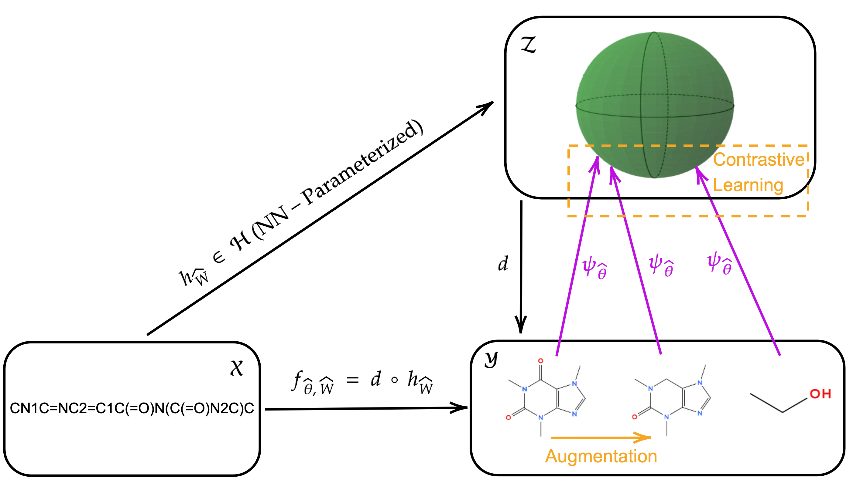
Figure 1: Illustration of ELE Framework.

The framework ELE illustrated in Figure 1 decomposes into 3 steps:

1. Obtain the feature map $\hat{\psi}$ by Contrastive Learning

2. At training time, solve surrogate regression with the resulting differentiable loss $\Delta_{\hat{\psi}}(y,h(x)):=\|h(x)-\hat{\psi}(y)\|^{2}_{\mathbb{R}^{d}}$

3. At inference time, decode the prediction in the surrogate space $\hat{h}(x)$ with the differentiable loss $\Delta_{\hat{\psi}}$.

We should note that the losses learned by ELE satisfy the ILE condition by definition. The reader can find in Section B of the Appendix a complete view of the ELE algorithm.

2.2.1 Feature Learning via Contrastive Learning.

The first step involves leveraging a set of output samples $\mathcal{S}_{n}=\{y_{i}\}_{i=1}^{n}\in\mathcal{Y}^{n}$ drawn from the marginal distribution $\mathbb{P}_{\mathsf{Y}}$ to learn the feature map $\psi$. We propose implementing the feature map as a parametric model such as a (deep) neural network defined by its generic parameter $\theta$. Of paramount importance here, is the differentiability of $\psi_{\theta}$ with respect to the structured variable. Indeed, we are not only interested in $\psi_{\theta}$ as a function of $y\in\mathcal{Y}$, but also require that, during inference, the feature map can be differentiable with respect to the structured variable. Therefore, we assume that we can relax a structured object $y\in\mathcal{Y}$ into a continuous object $\overline{y}\in\overline{\mathcal{Y}}$ by some invertible operator $\mathcal{R}:\mathcal{Y}\rightarrow\overline{\mathcal{Y}}$. Conversely if we consider an element $\overline{y}$ of $\overline{\mathcal{Y}}$, we can convert it back into $y:=\mathcal{R}^{-1}(\overline{y})$. It should be noted that $\mathcal{Y}\subset\overline{\mathcal{Y}}$. We give in Section 3 an example of relaxed representations of labeled graphs.

To learn $\psi_{\theta}:\overline{\mathcal{Y}}\rightarrow\mathbb{R}^{d}$, i.e., its parameter $\theta$, we leverage Contrastive Representation learning (CRL) (Chopra et al., 2005; Le-Khac et al., 2020), a technique that has been shown to give remarkable results in practice. In our problem, we have to define a mechanism to create similar pairs of output data $(y,y^{+})$ and dissimilar pairs $(y,y^{-})$ such that the CRL algorithm can learn the embedding $\psi_{\theta}$ by pulling together similar pairs $(\psi_{\theta}(y),\psi_{\theta}(y^{+}))$ while pushing apart dissimilar pairs $(\psi_{\theta}(y),\psi_{\theta}(y^{-}))$ in the feature space $\mathcal{Z}$.

Given constructed output data $\{(y_{i},y_{i}^{+},\{y_{i,k}^{-}\}_{k=1}^{K})\}_{i=1}^{n}$ where $y_{i}^{+}$ denotes the positive sample of $y_{i}$, $\{y_{i,k}^{-}\}_{k=1}^{K}$ denotes the negative ones of $y_{i}$, CRL aims at finding a NN-parameterized mapping $\psi_{\hat{\theta}}:\overline{\mathcal{Y}}\to\mathbb{S}^{d-1}$, where $\mathbb{S}^{d-1}\coloneqq\{x\in\mathbb{R}^{d}\;|\;\|{x}\|_{{\mathbb{R}^{d}}}=1\}$ denotes the unit $(d-1)$-sphere of radius 1, such that

$$\hat{\theta}\in\operatorname*{arg\,min}_{\theta\in\Theta}\frac{1}{m}\sum_{i=1}^{m}\ell_{\phi,\varphi}\left(\psi_{\theta}(y_{i}),\psi_{\theta}(y_{i}^{+}),\{\psi_{\theta}(y_{i,k}^{-})\}_{k=1}^{K}\right)$$ (5)

$$\mathrm{with}\quad\ell_{\phi,\varphi}(z,z^{+},\{z_{k}^{-}\}_{k=1}^{K})=\phi\left(\sum_{k=1}^{K}\varphi\left(-\langle{z},{z^{+}}\rangle_{{\mathbb{S}^{d-1}}}+\langle{z},{z_{k}^{-}}\rangle_{{\mathbb{S}^{d-1}}}\right)\right).$$ (6)

where $\phi$ and $\varphi$ are two given monotonously increasing and differentiable scalar functions.

Since the feature learning step involves only the output space, we are no longer limited to the labeled outputs of supervised data pairs. This allows us to leverage the abundance of unsupervised output data.

Output Neural Network Pre-Training (ONNPT).

Given a set of additional output samples $\tilde{\mathcal{S}}_{\tilde{n}}=\{y_{i}\}_{i=1}^{\tilde{n}}\in\mathcal{Y}^{\tilde{n}}$ from another distribution $\tilde{\mathbb{P}}_{\mathsf{Y}}$ close to $\mathbb{P}_{\mathsf{Y}}$, we first apply CRL on $\tilde{\mathcal{S}}_{\tilde{n}}$ with $T$ steps of SGD, then continue the learning procedure on the output data $\mathcal{S}_{n}=\{y_{i}\}_{i=1}^{n}\in\mathcal{Y}^{n}$ corresponding to our labelled set. One straightforward advantage of this technique is that it is usually easier to get access to unsupervised output data than input-output data pairs. This pre-training gives us a good initialization point for the output neural network weights.

Remark 2.1.

The paradigm of pre-training (Erhan et al., 2010) has gained great popularity since the introduction of large language models (Radford et al., 2018; Devlin et al., 2019; Liu et al., 2019). To solve a classic supervised learning problem with input-output pairs, a neural network is firstly trained on large-scale unlabelled input data with an unsupervised learning objective. Our work extends such a strategy to the output data space in the context of structured prediction.

Once the embedding $\psi_{\hat{\theta}}$ is obtained, we are then able to define the surrogate loss $\Delta_{\psi_{\hat{\theta}}}(y,h(x)):=\|\psi_{\hat{\theta}}(y)-h(x)\|^{2}$ and inject it in Equation 3.

2.2.2 Surrogate Regression with a Learned and Differentiable Loss

The fact that $\mathbb{S}^{d-1}\subset\mathbb{R}^{d}$ is of finite dimension $d$ enables us to parameterize the hypothesis space $\mathcal{H}$ with a deep neural network $u_{W}:\mathcal{X}\to\mathbb{R}^{d}$, whose parameter set is denoted by $W$, followed a $\ell_{2}$ normalization layer:

$$\mathcal{H}\coloneqq\{h_{W}(\cdot)=\frac{u_{W}(\cdot)}{\|{u_{W}(\cdot)}\|_{{\mathbb{R}^{d}}}}\mid u_{W}:\mathcal{X}\to\mathbb{R}^{d},W\in\mathcal{W}\}$$ (7)

The choice of neural network $u_{W}$ depends on the nature of input data. We will refer to this network as the backbone throughout the remainder of the paper. The hypothesis setting leads to the following optimization problem:

$$\min_{W\in\mathcal{W}}\frac{1}{n}\sum_{i=1}^{n}\|{h_{W}(x_{i})-\psi_{\hat{\theta}}(y_{i})}\|_{{\mathbb{R}^{d}}}^{2}.$$ (8)

Note that since for all $y\in\mathcal{Y}$, $\|{\psi_{\hat{\theta}}(y)}\|_{{\mathbb{R}^{d}}}=1$, the norm boils down to the negation of the following inner product: $\|{h_{W}(x)-\psi_{\hat{\theta}}(y)}\|_{{\mathbb{R}^{d}}}^{2}=2-2\langle h_{W}(x),\psi_{\hat{\theta}}(y)\rangle_{\mathbb{R}^{d}}$.

We can then turn to a Stochastic Gradient Descent (SGD) based algorithm (e.g., Adam Kingma and Ba (2015)) to obtain the surrogate estimator $h_{\hat{W}}$.

2.2.3 Decoding Based Inference

Given an input data point $x\in\mathcal{X}$, a prediction $\hat{z}$ in the surrogate space $\mathcal{Z}$ is first obtained through $h_{\hat{W}}$. It is then decoded back to the original output space $\mathcal{Y}$ through a suitable decoding function $d\in\mathcal{Y}^{\mathcal{Z}}$. Our final predictor of structured objects $f_{\hat{\theta},\hat{W}}:\mathcal{X}\to\mathcal{Y}$ is defined as follows:

$$f_{\hat{\theta},\hat{W}}(x)\coloneqq d\circ h_{\hat{W}}(x)$$ (9)

with

$$d(\hat{z})\in\operatorname*{arg\,min}_{y\in\mathcal{Y}}\|{\psi_{\hat{\theta}}(y)-\hat{z}}\|_{{\mathbb{R}^{d}}}^{2}=\operatorname*{arg\,max}_{y\in\mathcal{Y}}\langle{\psi_{\hat{\theta}}(y)},{\hat{z}}\rangle_{{\mathbb{R}^{d}}}$$ (10)

When a set of candidates $\mathcal{Y}^{c}=\{y_{1}^{c},\dots,y_{n_{c}}^{c}\}\subset\mathcal{Y}$ of finite size $n_{c}$ is given, we can compute the inner product score for each candidate, and the prediction is thus given by

$$f_{\hat{\theta},\hat{W}}(x)=y_{\hat{j}}^{c}\quad\text{where}\quad\hat{j}=\operatorname*{arg\,max}_{1\leq j\leq n_{c}}\langle{\psi_{\hat{\theta}}(y_{j}^{c})},{h_{\hat{W}}(x)}\rangle_{{\mathbb{R}^{d}}}.$$ (11)

We refer it as Candidate Selection decoding strategy. More generally, we are interested in exploiting the differentiability of the learned embedding due to the large size of the structured output space. We hence propose to solve the decoding problem described by Equation 10 by Gradient Descent.

Projected Gradient Descent Based Decoding (PGDBD).

Instead of considering the original discrete space $\mathcal{Y}$ as the constraint set of the optimization problem described by Equation 10, we optimize the objective function over its convex hull $\overline{\mathcal{Y}}$, and the prediction writes as a minimizer followed by the reverse operator $\mathcal{R}^{-1}$:

$$f_{\hat{\theta},\hat{W}}(x)=\mathcal{R}^{-1}\left(\operatorname*{arg\,min}_{\overline{y}\in\overline{\mathcal{Y}}}L_{x}(\overline{y})\right)\quad\text{with}\quad L_{x}(\overline{y})=\|{\psi_{\hat{\theta}}(\overline{y})-h_{\hat{W}}(x)}\|_{{\mathbb{R}^{d}}}^{2}$$ (12)

For the constrained problem described above, the Projected Gradient Descent method (or Projected Subgradiant Descent) can be used, since $\psi_{\hat{\theta}}$ is NN-parameterized and the squared norm is convex. With a step size $\eta$:

$$\tilde{y}^{(t+1)}=\overline{y}^{(t)}-\eta\nabla L_{x}(\overline{y}^{(t)}),\quad\overline{y}^{(t+1)}=\mathrm{P}_{\overline{\mathcal{Y}}}(\tilde{y}^{(t+1)})$$ (13)

where the projection operator $\mathrm{P}_{\overline{\mathcal{Y}}}$ finds the point in $\overline{\mathcal{Y}}$ closest to $\tilde{y}^{(t+1)}$.

The performance of a GD-based algorithm can be significantly improved using a suitable starting point. To reduce the number of gradient descent steps and obtain a better local minimum, we initialize the start point $y^{(0)}$ with the best prediction $y_{\hat{j}}^{c}$ of the candidate set as shown in Equation 11. When the candidate set is not given, we take the output labels of the training set $\mathcal{S}_{n}$ as the candidate set.

Projected Gradient Descent based decoding allows us to predict new structures which are not present in the training set while reducing the burden of designing a new decoder architecture each time when a new data structure is encountered.

3 Instantiation on Supervised Graph Prediction

In this section, we detail how to apply our framework in a concrete, non-trivial, Structured Prediction task: Supervised Graph Prediction (SGP). Given a data point from an arbitrary input space, SGP consists in predicting an output in a labeled graph space: we will describe this output space, how we apply the contrastive objective within it for feature learning, and how we relax it in order to apply our Projected Gradient Descent Based Decoding.

Output structured space: assuming nodes can be categorized into a set of discrete labels $\mathcal{T}$ of size $T$, edges into a set of labels $\mathcal{S}$ of size $S$ (with no edge being considered as one of the edge labels), each graph of at most $m_{\mathrm{max}}$ nodes can be represented by a node feature list $\mathrm{F}$ and an edge feature matrix $\mathrm{E}$, which forms a labeled graph space $\mathcal{G}^{\mathcal{T},\mathcal{S}}$ which is written as follows:

$$\mathcal{G}^{\mathcal{T},\mathcal{S}}\coloneqq\bigcup_{m=1}^{m_{\mathrm{max}}}\mathcal{G}_{m}^{\mathcal{T},\mathcal{S}}\quad\text{with}$$

$$\mathcal{G}_{m}^{\mathcal{T},\mathcal{S}}\coloneqq\{(\mathrm{F},\mathrm{E})\mid\mathrm{F}\in\mathcal{T}^{m},\;\mathrm{E}\in\mathcal{S}^{m\times m},\mathrm{E}_{i,j}=\mathrm{E}_{j,i},\forall(i,j)\in\llbracket 1,m\rrbracket^{2}\}$$ (14)

where $F_{i}$ represents the label of node $i$ and $E_{i,j}$ represents the label of edge between the node $i$ and $j$. As working on a graph space of various node sizes is difficult in practice, we introduce virtual nodes $v$ into graphs so that each graph contains $m_{\mathrm{max}}$ nodes. The virtual node is treated as an additional node label, and the new graph has no edge linking to the virtual nodes. We consider thus the new padded graph space $\mathcal{G}_{m_{\mathrm{max}}}^{\mathcal{T}\cup\{v\},\mathcal{S}}$ as the final output structured space $\mathcal{\mathcal{Y}}$.

We define a continuous relaxation $\overline{\mathcal{G}}_{m_{\mathrm{max}}}^{\mathcal{T}\cup\{v\},\mathcal{S}}$ (which we will denote by $\overline{\mathcal{G}}$ for the simplification) of $\mathcal{G}_{m_{\mathrm{max}}}^{\mathcal{T}\cup\{v\},\mathcal{S}}$ as follows:

$$\overline{\mathcal{G}}:=\{(\mathrm{F},\mathrm{E})\mid\mathrm{F}\in(\Delta^{T})^{m_{\mathrm{max}}},\mathrm{E}\in(\Delta^{S-1})^{m_{\mathrm{max}}\times m_{\mathrm{max}}},\mathrm{E}_{i,j}=\mathrm{E}_{j,i},\forall(i,j)\in\llbracket 1,m_{\mathrm{max}}\rrbracket^{2}\}$$ (15)

where $\Delta^{S-1}$ denotes a simplex of dimension $S-1$ in $\mathbb{R}^{S}$. Then the relaxing operator $\mathcal{R}:\mathcal{Y}\rightarrow\overline{\mathcal{Y}}$ consists in simply mapping each node label and edge label with one-hot encoding.

Contrastive learning: given a graph $g={(\mathrm{F},\mathrm{E})}\in\overline{\mathcal{G}}$, we adopt node dropping (i.e., randomly discarding a certain portion of vertices along with their connections) introduced by You et al. (2020) to create the positive sample $g^{+}$. In practice, we replace the nodes to be dropped by the virtual nodes so that the augmented graph $g^{+}$ lives in the same space of $g$. The augmented graphs of random graphs in the dataset are chosen to be the negative samples $\{g_{k}^{-}\}_{k=1}^{K}$. Graph Neural Networks (GNNs) (Kipf and Welling, 2017; Gilmer et al., 2017) are ubiquitous choices to parameterize $\psi_{\theta}:\overline{\mathcal{G}}\to\mathbb{S}^{d-1}$. We adopt Relational Graph Convolutional Networks (R-GCNs) (Schlichtkrull et al., 2018), followed by a sum pooling layer, a MLP layer and a $\ell_{2}$ normalization layer. Each layer of R-GCNs does the following operation:

$$\mathrm{F}^{(l+1)}=\sigma(\sum_{s=1}^{S}\mathrm{E}_{,:,:s}\mathrm{F}^{(l)}W_{c,:,:})$$ (16)

where $\sigma$ denotes an activation function and the tensor $W\in\mathbb{R}^{S\times d\times d}$ contains the parameters of the layer except for the first layer where we have $W\in\mathbb{R}^{S\times(T+1)\times d}$. Our motivation for choosing R-GCNs is twofold: first, the above layer operation is (sub)differentiable with respect to both $\mathrm{E}$ and $\mathrm{F}$; second, it integrates the information of edge features. The output neural network $\psi_{\theta}$ are then trained to minimize the popular InfoNCE loss (Sohn, 2016; Oord et al., 2018; Chen et al., 2020):

$$\ell_{\mathrm{InfoNCE}}(z,z^{+},\{z_{k}^{-}\}_{k=1}^{K}) =\tau\log\left(\epsilon+\sum_{k=1}^{K}\exp\left(\frac{\langle{z},{z_{k}^{-}}\rangle_{{\mathbb{S}^{d-1}}}-\langle{z},{z^{+}}\rangle_{{\mathbb{S}^{d-1}}}}{\tau}\right)\right)$$ (17)

where $\epsilon>0$ is an arbitrary constant and $\tau>0$ is a scalar temperature hyperparameter.

Projected gradient descent based decoding: The following proposition details how to conduct the projection operation $P_{\overline{\mathcal{G}}}(\cdot)$ during gradient descent.

Proposition 3.1 (Projected Gradient Descent on Relaxed Graph Space).

Suppose that $(\hat{\mathrm{F}},\hat{\mathrm{E}})$ are the projections of $(\tilde{\mathrm{F}},\tilde{\mathrm{E}})\in\mathbb{R}^{m_{\mathrm{max}}\times(T+1)}\times\mathbb{R}^{m_{\mathrm{max}}\times m_{\mathrm{max}}\times S}$ on $\overline{\mathcal{G}}$; then, $(\hat{\mathrm{F}},\hat{\mathrm{E}})$ are the solutions of the following optimization problems:

$$\forall(i,j)\in\llbracket 1,m_{\mathrm{max}}\rrbracket^{2},\hat{\mathrm{F}}_{i}=\operatorname*{arg\,min}_{a\in\mathbb{R}^{(T+1)}}\|{a-\tilde{\mathrm{F}}_{i}}\|_{{\mathbb{R}^{(T+1)}}}^{2}\quad\mathrm{s.t.},\;{a}^{\mathsf{T}}\mathds{1}_{T+1}=1,\;a\geq 0$$ (18)

$$\hat{\mathrm{E}}_{i,j}=\hat{\mathrm{E}}_{j,i}=\operatorname*{arg\,min}_{b\in\mathbb{R}^{S}}\|{b-(\tilde{\mathrm{E}}_{i,j}+\tilde{\mathrm{E}}_{j,i})/2}\|_{{\mathbb{R}^{S}}}^{2}\quad\mathrm{s.t.},\;{b}^{\mathsf{T}}\mathds{1}_{S}=1,\;b\geq 0$$ (19)

The proof can be found in Appendix A. With the above proposition, we have successfully decomposed the original projection operation into a series of Euclidean projections onto the simplex, which can be independently and efficiently solved by the algorithm proposed in Duchi et al. (2008). Furthermore, since all $\mathrm{F}$ and all $\mathrm{E}$ are of the same shape, we can compute the decoding loss in a batch fashion, and then update them through the backpropagation, which accelerates largely the decoding procedure.

The final step consists in using reverse operator $\mathcal{R}^{-1}$ to put the prediction $\overline{g}\in\overline{\mathcal{G}}$ back to the original discrete space $\mathcal{G}^{\mathcal{T},\mathcal{S}}$. We first use argmax operator to transform each feature simplex to a discrete label for both nodes and edges. Then we delete the nodes whose label is virtual along with their edges.

4 Related Works

4.1 Contrastive Learning of Structured Data Embedding

While contrastive learning has long been used to facilitate learning when the output space is too large to be effectively handled, its popularity has exploded for the unsupervised learning of structured objects in the last few years. In particular, sentences (sequences of tokens) are discrete objects for which contrastive learning is a popular embedding method: an early example, Quick Thoughts (Logeswaran and Lee, 2018) encourages sentences within the same context to be close in the embedding space while maximizing the distance between sentences from different contexts. SBERT (Reimers and Gurevych, 2019) selects sentences from the same section of an article as positive samples and those from different sections as negative samples. On the other hand, SimCSE (Gao et al., 2021) and most of the numerous approaches that followed generate positive samples by applying a different dropout mask to intermediate representations, rather than discrete operations. Similarly, there exists extensive literature on the unsupervised learning of graph embeddings through contrastive learning. Again, many variants have been explored: for creating positive samples, GraphCL (You et al., 2020) designs four types of graph augmentations (node dropping, edge perturbation, attribute masking and subgraph), while MVGRL (Hassani and Khasahmadi, 2020) creates two views of the same graph through diffusion and sub-sampling operations. Other approaches contrast local and global views of the graph, such as InfoGraph (Sun et al., 2020), which maximises mutual information between representations of patches of the graph. These methods usually employ GNNs to learn such embeddings. For more details, we refer the reader to a recent survey on the contrastive learning of graphs, such as Ju et al. (2024).

4.2 Connections with Previous Structured Prediction Methods

Our proposed framework has strong links to several previous works focusing on structured prediction. First, Input Output Kernel Regression (IOKR) (Brouard et al., 2016) defines a scalar-valued kernel on the structured output, where the loss function corresponds to the canonical Euclidean distance induced by the kernel features. Implicit Loss Embedding (ILE) (Ciliberto et al., 2016, 2020) generalizes this idea to any loss function that satisfies the ILE condition. However, both methods introduce an implicit surrogate embedding space whose dimension is often unknown or can be infinite, necessitating nonparametric methods, such as those based on input operator-valued kernels (Micchelli and Pontil, 2005), to solve the surrogate regression problems. Moreover, IOKR and ILE are limited to tasks where the decoding problem can still be solved in a reasonable time using approximation algorithms, such as the ranking, or where a set of candidates is provided. A second set of recent works have addressed these limitations: for example, ILE-FGW (Brogat-Motte et al., 2022) and ILE-FNGW (Yang et al., 2024) have applied the framework to highly structured graph objects, leveraging differentiable loss functions based on Optimal Transport theory. The novel graph structures can also be predicted in a gradient descent decoding way. DSOKR (El Ahmad et al., 2024b) reduces the dimensionality of the infinite-dimensional feature space by a sketching (Mahoney, 2011; Woodruff, 2014) version of Kernel Principal Component Analysis (KPCA) (Schölkopf et al., 1997), which enables the use of neural networks to predict representations within this subspace. However, all of those methods rely on pre-defined losses, which are not systematically differentiable and computationally efficient for each data type. In contrast, our framework ELE allows learning a differentiable surrogate loss tailored to each data set, and the explicit nature of the output embedding permits training the input neural network without the need for additional dimensionality reduction techniques.

Finally, our Gradient Descent Based Decoding for the pre-image problem, which goes beyond the candidate set to make a prediction, is related to Structured Prediction Energy Networks (SPEN) (Belanger and McCallum, 2016) if we consider $\|{\psi_{\hat{\theta}}(\cdot)-h_{\hat{\theta^{\prime}}}(x)}\|_{{\mathbb{R}^{d}}}^{2}$ as the energy function $E_{x}(\cdot)$. However, while the contribution of SPEN is limited to multi-label output spaces, we extend it to general graph output spaces. Furthermore, we also propose an initialization strategy dedicated to dealing with this more complex output space.

5 Experiments

5.1 SMILES to QM9

We demonstrate the applicability of our method through a graph prediction task, choosing to predict graphs of molecules given their string description.

Dataset

We use the QM9 molecule dataset (Ruddigkeit et al., 2012; Ramakrishnan et al., 2014), containing around 130,000 small organic molecules. These molecules were processed using RDKit, with aromatic rings converted to their Kekule form and hydrogen atoms removed. We also removed molecules containing only one atom. Each molecule contains up to 9 atoms of Carbon, Nitrogen, Oxygen, or Fluorine, along with three types of bonds: single, double, and triple. As input features, we use the Simplified Molecular Input Line-Entry System (SMILES), which are strings describing their chemical structure. We refer to the resulting dataset as SMI2Mol.

Task

Our task is to predict an output molecule graph $y\in\mathcal{Y}$ from the corresponding input string $x\in\mathcal{X}$. The performance is measured using Graph Edit Distance (GED) between the predicted molecule and the true molecule, implemented by the NetworkX package (Hagberg et al., 2008). Besides showing the performance of our method ELE against baselines, we investigate in detail several decoding strategies to explore the usefulness of our Projected Gradient Based Decoding.

5.1.1 Experimental Settings

In our dataset, the space of molecules is represented as the graph space $\mathcal{G}^{\mathcal{T},\mathcal{S}}$ described in Equation 14 where $\mathcal{T}$ is a set of atom types and $\mathcal{T}$ is a set of bond types (including non-existence of bond). All the graphs are padded to graphs of $m_{\mathrm{max}}=9$ nodes.

Output embedding model: As stated in Section 3, we parameterize our output neural network $\psi_{\theta}$ with R-GCNs (Schlichtkrull et al., 2018).

Output embedding learning: In the default setting, contrastive learning is conducted only on the graphs from QM9 training set. In the setting of Output Neural Network Pre-training (ONNP), we use GDB-11 (Fink et al., 2005; Fink and Reymond, 2007) as the pre-training dataset, which enumerates 26,434,571 small organic molecules up to 11 atoms of Carbon, Nitrogen, Oxygen, or Fluorine. Hence, we pad all the molecules, including those from QM9, into the graphs of size $m_{\mathrm{max}}=11$.

Input space and regression model: To parameterize the output neural network $h_{\theta^{\prime}}$, we use a multi-layer Transformer encoder (Vaswani et al., 2017). The SMILES strings are tokenized into character sequences as inputs for the Transformer encoder, with the maximum length set to 25.

Decoding: If unspecified, the decoding is made by looking for the most appropriate candidate in $\mathcal{Y}^{c}$, as described at the beginning of Section 2.2.3. To experiment with our proposed Projected Gradient Descent Based Decoding (PGDBD), we look into three decoding configurations:

1. Candidate selection from $\mathcal{Y}^{c}$, as above.

2. The predicted molecule is obtained using PGDBD, initialized with a random molecule from $\mathcal{Y}^{c}$.

3. The predicted molecule is obtained using PGDBD, initialized with the best candidate molecule obtained from strategy 1.

We create five dataset splits using different seeds from the full set of SMILES-molecule pairs. Each split contains 131,382 training samples, 500 validation samples, and 2,000 test samples. The details about the values of the hyperparameters or their search ranges can be found in Appendix C.

5.1.2 Results

Table 1: Graph Edit Distance of different methods on SMI2Mol test set.

	GED w/o edge feature $\downarrow$	GED w/ edge feature $\downarrow$
SISOKR	$3.330\pm 0.080$	$4.192\pm 0.109$
NNBary-FGW	$5.115\pm 0.129$	-
Sketched ILE-FGW	$2.998\pm 0.253$	-
DSOKR	$\bm{1.951\pm 0.074}$	$2.960\pm 0.079$
ELE	$2.305\pm 0.033$	$2.444\pm 0.039$
ELE w/ ONNPT	$2.164\pm 0.058$	$2.291\pm 0.083$
ELE w/ ONNPT + PGDBD	$2.131\pm 0.075$	$\bm{2.252\pm 0.102}$

Comparison with Baseline Models.

Our method is benchmarked against SISOKR (El Ahmad et al., 2024a), NNBary-FGW (Brogat-Motte et al., 2022), ILE-FGW (Brogat-Motte et al., 2022), and DSOKR (El Ahmad et al., 2024b). The results are presented in Table 1. From them, we observe that ELE obtains better performance in terms of GED with edge features and competitive performance in terms of GED without edge features. The results also demonstrate the relevance of pre-training the output neural network with additional output data. However, there is no obvious performance improvement provided by PGDBD; we hence perform supplementary experiments with supplementary decoding strategies.

Study of Projected Gradient Descent Based Decoding Strategy.

In this section, we study our proposed PGDBD strategy under the three configurations outlined in the previous section. At the same time, we vary the size of the candidate set: in each experiment, a specific proportion of the training molecules is used to form the candidate set, controlled by a predefined ratio. In addition to the Graph Edit Distance (GED) metric, we also calculate the number of perfectly predicted outputs, which are examples for which the GED between the predicted molecule and the ground truth molecule is zero. Results on the test set are shown in Figure 2.

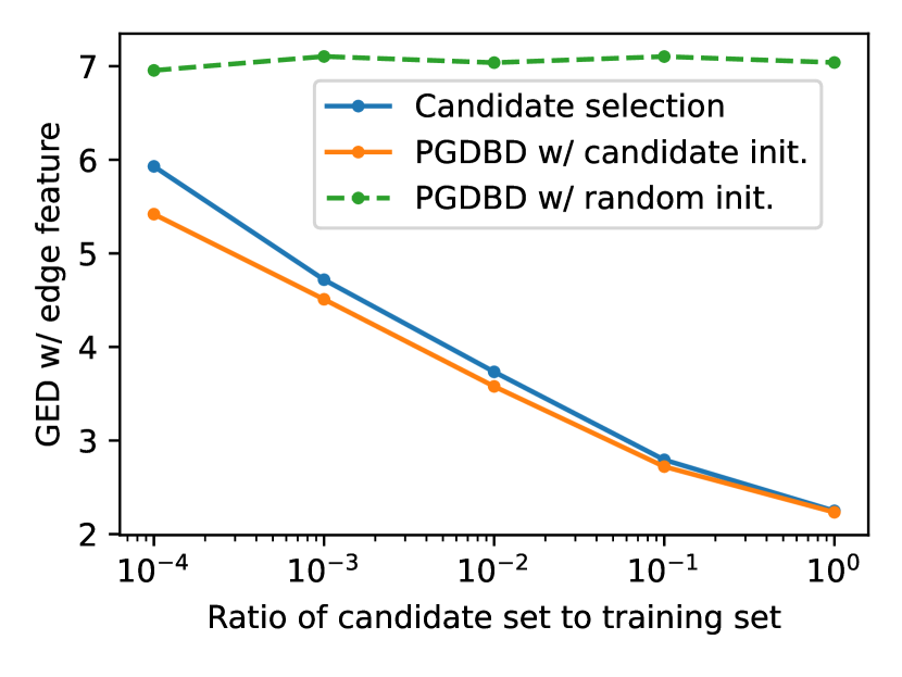
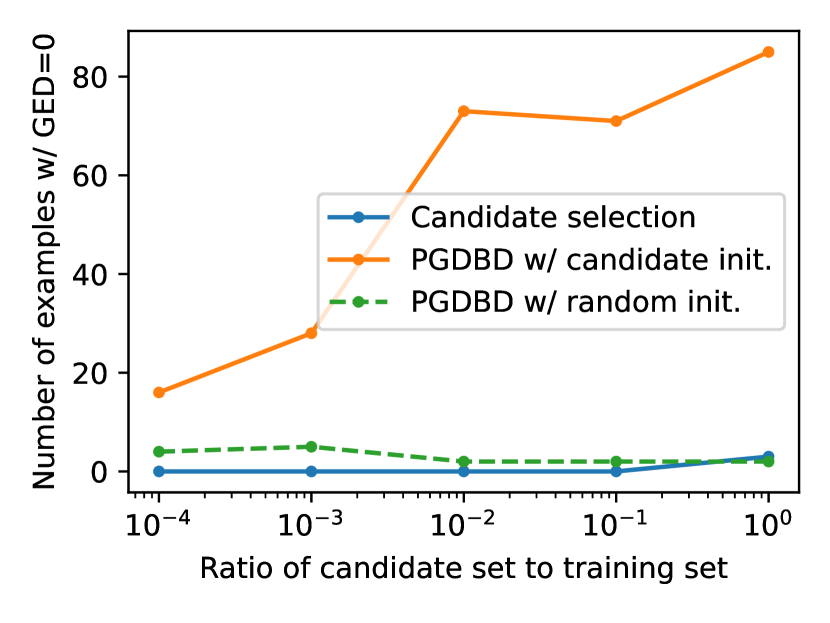
Figure 2: (Left) The GED with edge features of DIDOR under different decoding strategies with various sizes of candidate set. (Right) The number of predictions whose GED with the ground truth is zero, obtained by DIDOR under different decoding strategies with various sizes of candidate set.

From the GED values displayed in the left figure, we can make two key observations. First, the performance of the PGDBD strategy improves significantly when a good graph is selected from the candidate set for initialization, rather than being drawn randomly. Second, when the size of the candidate set is limited, PGDBD enhances the quality of predictions by refining the selected candidate molecules. However, this effect becomes less pronounced as the candidate set size increases. We conjecture that a candidate graph with the highest inner product score may already be situated in a favorable local minimum, especially when considering the entire training set as $\mathcal{Y}^{c}$. We also posit that the highly non-convex nature of $\psi_{\theta}$ renders the optimization difficult. The right figure, on the other hand, demonstrates the ability of our proposed PGDBD strategy to predict novel graph structures, which is impossible by simply selecting the best candidate.

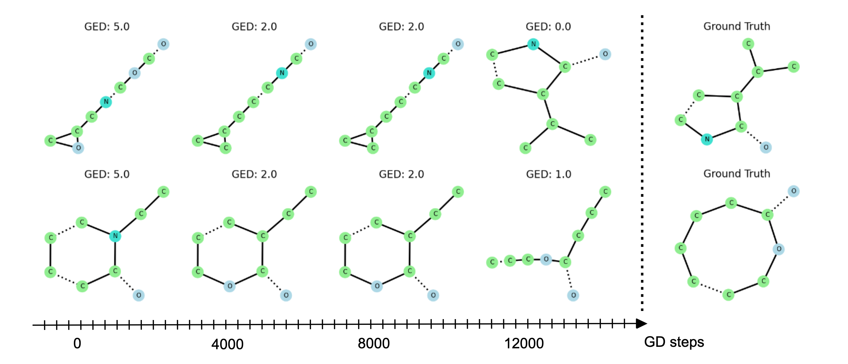
Figure 3: Update of the predicted molecules along with the projected gradient descent.

Finally, we display in Figure 3 some examples of how predicted molecules, as parameters, initialized with a random molecule, are updated through the projected gradient descent steps. We can clearly observe a phenomenon of convergence even in its original discrete space.

6 Conclusion

In this work, we have introduced a novel framework, Explicit Loss Embedding, for addressing Structured Prediction tasks by leveraging contrastive learning within the Surrogate Regression setting. By building a differentiable surrogate loss from explicit embeddings learned directly from output data, our method circumvents the need for manually defining complex and often non-differentiable loss functions tailored to each structured outputs. Our empirical results, in the context of text-to-graph predictions, demonstrate that ELE performs on par with or surpasses other surrogate regression methods reliant on pre-defined losses. Furthermore, taking advantage of the differentiability of the surrogate loss, we propose a projected gradient descent based technique for decoding. Despite the challenge of solving a highly non-convex constrained optimization problem, our technique demonstrates the preliminary ability to predict novel graph structures, opening the door for enhancing prediction quality by incorporating more advanced optimization techniques in future work.

Appendix A Proof of Proposition 3.1

Proof.

The projection on such graph space of a point $\tilde{y}=(\tilde{\mathrm{E}},\tilde{\mathrm{F}})$ solves actually the follwoing optimization problem:

$$(\hat{\mathrm{F}},\hat{\mathrm{E}}) =\mathrm{P}_{\overline{\mathcal{G}}}((\tilde{\mathrm{E}},\tilde{\mathrm{F}}))$$ (20)

$$=\operatorname*{arg\,min}_{\mathrm{F}\in(\Delta^{T})^{m_{\mathrm{max}}},\mathrm{E}\in(\Delta^{S-1})^{m_{\mathrm{max}}\times m_{\mathrm{max}}},\mathrm{E}_{i,j}=\mathrm{E}_{j,i}}\|{\mathrm{E}-\tilde{\mathrm{E}}}\|_{{F}}^{2}+\|{\mathrm{F}-\tilde{\mathrm{F}}}\|_{{F}}^{2}$$ (21)

$$=\operatorname*{arg\,min}_{\mathrm{F}\in(\Delta^{T})^{m_{\mathrm{max}}},\mathrm{E}\in(\Delta^{S-1})^{m_{\mathrm{max}}\times m_{\mathrm{max}}},\mathrm{E}_{i,j}=\mathrm{E}_{j,i}}\sum_{i,j}\|{\mathrm{E}_{i,j}-\tilde{\mathrm{E}}_{i,j}}\|_{{\mathbb{R}^{S}}}^{2}+\sum_{i}\|{\mathrm{F}_{i}-\tilde{\mathrm{F}}_{i}}\|_{{\mathbb{R}^{T+1}}}^{2}$$ (22)

We can easily conclude that for any $(i,j)\in\llbracket 1,m_{\mathrm{max}}\rrbracket^{2}$, we have

$$\hat{\mathrm{F}}_{i}=\operatorname*{arg\,min}_{a\in\mathbb{R}^{T+1}}\|{a-\tilde{\mathrm{F}}_{i}}\|_{{\mathbb{R}^{T+1}}}^{2}\quad\mathrm{s.t.},\;{a}^{\mathsf{T}}\mathds{1}_{T+1}=1,\;a\geq 0$$ (23)

$$\hat{\mathrm{E}}_{i,j}=\hat{\mathrm{E}}_{j,i}=\operatorname*{arg\,min}_{b\in\mathbb{R}^{S}}\|{b-\tilde{\mathrm{E}}_{i,j}}\|_{{\mathbb{R}^{S}}}^{2}+\|{b-\tilde{\mathrm{E}}_{j,i}}\|_{{\mathbb{R}^{S}}}^{2}\quad\mathrm{s.t.},\;{b}^{\mathsf{T}}\mathds{1}_{S}=1,\;b\geq 0$$ (24)

Furthermore, it can be shown from Equation 24 that

$$\hat{\mathrm{E}}_{i,j}=\hat{\mathrm{E}}_{j,i}=\operatorname*{arg\,min}_{b\in\mathbb{R}^{S}}\|{b-(\tilde{\mathrm{E}}_{i,j}+\tilde{\mathrm{E}}_{j,i})/2}\|_{{\mathbb{R}^{S}}}^{2}\quad\mathrm{s.t.},\;{b}^{\mathsf{T}}\mathds{1}_{S}=1,\;b\geq 0$$ (25)

which projects the point $(\tilde{\mathrm{E}}_{i,j}+\tilde{\mathrm{E}}_{j,i})/2$ on the simplex space. ∎

Appendix B Pseudo-code of the ELE algorithm

input : Training set$\{(x_{i},y_{i})\}_{i=1}^{n}$, validation set$\{(x_{i}^{\mathrm{val}},y_{i}^{\mathrm{val}})\}_{i=1}^{n_{\mathrm{val}}}$, test inputs $\{x_{i}^{\mathrm{te}}\}_{i=1}^{n_{\mathrm{te}}}$, candidate set $\{y_{i}^{\mathrm{c}}\}_{i=1}^{n_{\mathrm{c}}}$, additional output training set $\{y_{i}\}_{i=1}^{\tilde{n}}$

output : Predictions $\{\hat{y}_{i}\}_{i=1}^{n_{\mathrm{te}}}$ of the test inputs

init : Number of pre-training steps of the output NN $T_{1}$, number of PGDBD steps $T_{2}$

// 1. Training

// 1.a. Training of output NN $\psi_{\theta}$: contrastive learning of the explicit embedding

$\bullet$ Pre-Train output neural network $\psi_{\theta}$ on $\{y_{i}\}_{i=1}^{\tilde{n}}$ with $T_{1}$ setps of gradient descent.

$\bullet$ Fine-Tune output neural network $\psi_{\theta}$ on $\{y_{i}\}_{i=1}^{n}$ with early stopping.

// 1.b. Training of input NN $h_{W}$: addressing surrogate problem

$\bullet$ Obtain the explicit embedding $\{\psi_{\hat{\theta}}(y_{i})\in\mathbb{S}^{d-1}\}_{i=1}^{n}$ of the training output, and the ones $\{\psi_{\hat{\theta}}(y_{i}^{\mathrm{val}})\in\mathbb{S}^{d-1}\}_{i=1}^{n_{\mathrm{val}}}$ of the validation output.

$\bullet$ Solve $\hat{W}=\operatorname*{arg\,min}_{W\in\mathcal{W}}\frac{1}{n}\sum_{i=1}^{n}\|{h_{W}(x_{i})-\psi_{\hat{\theta}}(y_{i})}\|_{{\mathcal{Z}}}^{2}$ by Adam optimizer, with early stopping based on mean squared error on validation set $\{(x_{i}^{\mathrm{val}},\psi_{\hat{\theta}}(y_{i}^{\mathrm{val}}))\}_{i=1}^{n_{\mathrm{val}}}$.

// 2. Inference

$\bullet$ Obtain the explicit embedding $\{\psi_{\hat{\theta}}(y_{i}^{\mathrm{c}})\in\mathbb{S}^{d-1}\}_{i=1}^{n_{\mathrm{c}}}$ of the candidates set

$\bullet$ Initialize the predictions $\{y^{(0)}_{i}\}_{i=1}^{n_{\mathrm{te}}}$ of the test inputs $\{x_{i}^{\mathrm{te}}\}_{i=1}^{n_{\mathrm{te}}}$ with the best candidate:

$\{y^{(0)}_{i}=y_{\hat{j}}^{c}\mid\hat{j}=\operatorname*{arg\,max}_{1\leq j\leq n_{c}}\langle{\psi_{\hat{\theta}}(y_{j}^{c})},{h_{\hat{W}}(x_{i}^{\mathrm{te}})}\rangle_{{\mathbb{R}^{d}}}\}_{i=1}^{n_{\mathrm{te}}}$

$\bullet$ Update the predictions by $T_{2}$ steps of projected gradient descent to solve the problem: $\forall i\in\llbracket 1,n_{\mathrm{te}}\rrbracket,\;\hat{y}_{i}=\mathcal{R}^{-1}\left(\operatorname*{arg\,min}_{\overline{y}\in\overline{\mathcal{Y}}}\|{\psi_{\hat{\theta}}(\overline{y})-h_{\hat{W}}(x)}\|_{{\mathbb{R}^{d}}}^{2}\right)$.

Algorithm 1 Explicit Loss Embedding (ELE)

The framework ELE is summarized in Algorithm 1.

Appendix C Hyperparameters Details

Table 2, Table 3 and Table 4 present the details about the values of the hyperparameters or their search ranges on SMI2Mol dataset with ELE framework.

Table 2: Contrastive learning hyper-parameters or their searching ranges during the cross-validation on SMI2Mol dataset.

Hyper-parameters	Searching ranges
Node dropping rate	$0.05$
SGD batch size	512
SGD learning rate	$10^{-3}$
Number of R-GCN layers	$\{2,4,6\}$
Hidden dimension of R-GCN	$\{32,64,128,256,512\}$
Number of pre-training steps	640,000

Table 3: Surrogate regression hyper-parameters or their searching ranges during the cross-validation on SMI2Mol dataset.

Hyper-parameters	Searching ranges
SGD batch size	128
SGD learning rate	$10^{-3}$
Number of Transformer layers	$\{2,4,6\}$
Hidden dimension of Transformer	$\{32,64,128,256,512\}$
Number of heads of Attention in Transformer	$\{2,4,8\}$
Dropout rate of Transformer layers	0

Table 4: PGDBD hyper-parameters or their searching ranges during the cross-validation on SMI2Mol dataset.

Hyper-parameters	Searching ranges
PGD number of steps	{ 2000, 4000, 6000, 8000, 10000, 12000 }
PGD step size	$\{0.1,1,10\}$

References

- Bakir et al. (2007) G. Bakir, T. Hofmann, B. Schoelkopf, A. J. Smola, B. Taskar, and S. Vishwanathan, editors. Predicting Structured Data. The MIT Press, July 2007. ISBN 978-0-262-25569-1.
- Belanger and McCallum (2016) D. Belanger and A. McCallum. Structured Prediction Energy Networks. In M. F. Balcan and K. Q. Weinberger, editors, Proceedings of The 33rd International Conference on Machine Learning, volume 48 of Proceedings of Machine Learning Research, pages 983–992, New York, New York, USA, June 2016. PMLR.
- Bellet et al. (2013) A. Bellet, A. Habrard, and M. Sebban. A Survey on Metric Learning for Feature Vectors and Structured Data. CoRR, abs/1306.6709, 2013. arXiv: 1306.6709.
- Borgwardt et al. (2020) K. Borgwardt, E. Ghisu, F. Llinares-López, L. O’Bray, and B. Rieck. Graph Kernels: State-of-the-Art and Future Challenges. Foundations and Trends® in Machine Learning, 13(5-6):531–712, 2020. ISSN 1935-8237.
- Brogat-Motte et al. (2022) L. Brogat-Motte, R. Flamary, C. Brouard, J. Rousu, and F. D’Alché-Buc. Learning to Predict Graphs with Fused Gromov-Wasserstein Barycenters. In K. Chaudhuri, S. Jegelka, L. Song, C. Szepesvari, G. Niu, and S. Sabato, editors, Proceedings of the 39th International Conference on Machine Learning, volume 162 of Proceedings of Machine Learning Research, pages 2321–2335. PMLR, July 2022.
- Brouard et al. (2016) C. Brouard, M. Szafranski, and F. d’Alché Buc. Input Output Kernel Regression: Supervised and Semi-Supervised Structured Output Prediction with Operator-Valued Kernels. Journal of Machine Learning Research, 17(176):1–48, 2016.
- Chechik et al. (2010) G. Chechik, V. Sharma, U. Shalit, and S. Bengio. Large Scale Online Learning of Image Similarity Through Ranking. J. Mach. Learn. Res., 11:1109–1135, Mar. 2010. ISSN 1532-4435. Publisher: JMLR.org.
- Chen et al. (2020) T. Chen, S. Kornblith, M. Norouzi, and G. Hinton. A Simple Framework for Contrastive Learning of Visual Representations. In H. D. III and A. Singh, editors, Proceedings of the 37th International Conference on Machine Learning, volume 119 of Proceedings of Machine Learning Research, pages 1597–1607. PMLR, July 2020.
- Chopra et al. (2005) S. Chopra, R. Hadsell, and Y. LeCun. Learning a Similarity Metric Discriminatively, with Application to Face Verification. In 2005 IEEE Computer Society Conference on Computer Vision and Pattern Recognition (CVPR’05), volume 1, pages 539–546 vol. 1, 2005.
- Ciliberto et al. (2016) C. Ciliberto, L. Rosasco, and A. Rudi. A Consistent Regularization Approach for Structured Prediction. In D. Lee, M. Sugiyama, U. Luxburg, I. Guyon, and R. Garnett, editors, Advances in Neural Information Processing Systems, volume 29. Curran Associates, Inc., 2016.
- Ciliberto et al. (2020) C. Ciliberto, L. Rosasco, and A. Rudi. A General Framework for Consistent Structured Prediction with Implicit Loss Embeddings. Journal of Machine Learning Research, 21(98):1–67, 2020.
- Cortes et al. (2005) C. Cortes, M. Mohri, and J. Weston. A general regression technique for learning transductions. In L. D. Raedt and S. Wrobel, editors, Machine Learning, Proceedings of the Twenty-Second International Conference (ICML 2005), Bonn, Germany, August 7-11, 2005, volume 119 of ACM International Conference Proceeding Series, pages 153–160. ACM, 2005.
- Cortes et al. (2010) C. Cortes, M. Mohri, and A. Rostamizadeh. Two-Stage Learning Kernel Algorithms. In Proceedings of the 27th Annual International Conference on Machine Learning (ICML 2010), 2010.
- Devlin et al. (2019) J. Devlin, M.-W. Chang, K. Lee, and K. Toutanova. BERT: Pre-training of Deep Bidirectional Transformers for Language Understanding. In Proceedings of the 2019 Conference of the North American Chapter of the Association for Computational Linguistics: Human Language Technologies (NACCL-HLT), pages 4171–4186, June 2019.
- Duchi et al. (2008) J. Duchi, S. Shalev-Shwartz, Y. Singer, and T. Chandra. Efficient Projections onto the l1-Ball for Learning in High Dimensions. In Proceedings of the 25th International Conference on Machine Learning, ICML ’08, pages 272–279, New York, NY, USA, 2008. Association for Computing Machinery. ISBN 978-1-60558-205-4. event-place: Helsinki, Finland.
- El Ahmad et al. (2024a) T. El Ahmad, L. Brogat-Motte, P. Laforgue, and F. d’Alché Buc. Sketch In, Sketch Out: Accelerating both Learning and Inference for Structured Prediction with Kernels. In S. Dasgupta, S. Mandt, and Y. Li, editors, Proceedings of The 27th International Conference on Artificial Intelligence and Statistics, volume 238 of Proceedings of Machine Learning Research, pages 109–117. PMLR, May 2024a.
- El Ahmad et al. (2024b) T. El Ahmad, J. Yang, P. Laforgue, and F. d’Alché Buc. Deep Sketched Output Kernel Regression for Structured Prediction. In A. Bifet, J. Davis, T. Krilavičius, M. Kull, E. Ntoutsi, and I. Žliobaitė, editors, Machine Learning and Knowledge Discovery in Databases. Research Track, pages 93–110, Cham, 2024b. Springer Nature Switzerland. ISBN 978-3-031-70352-2.
- Erhan et al. (2010) D. Erhan, Y. Bengio, A. Courville, P.-A. Manzagol, P. Vincent, and S. Bengio. Why Does Unsupervised Pre-training Help Deep Learning? Journal of Machine Learning Research, 11(19):625–660, 2010.
- Fink and Reymond (2007) T. Fink and J.-L. Reymond. Virtual Exploration of the Chemical Universe up to 11 Atoms of C, N, O, F: Assembly of 26.4 Million Structures (110.9 Million Stereoisomers) and Analysis for New Ring Systems, Stereochemistry, Physicochemical Properties, Compound Classes, and Drug Discovery. Journal of Chemical Information and Modeling, 47(2):342–353, Mar. 2007. ISSN 1549-9596. Publisher: American Chemical Society.
- Fink et al. (2005) T. Fink, H. Bruggesser, and J.-L. Reymond. Virtual Exploration of the Small-Molecule Chemical Universe below 160 Daltons. Angewandte Chemie International Edition, 44(10):1504–1508, Feb. 2005. ISSN 1433-7851. Publisher: John Wiley & Sons, Ltd.
- Gao et al. (2021) T. Gao, X. Yao, and D. Chen. SimCSE: Simple Contrastive Learning of Sentence Embeddings. In M.-F. Moens, X. Huang, L. Specia, and S. W.-t. Yih, editors, Proceedings of the 2021 Conference on Empirical Methods in Natural Language Processing, pages 6894–6910, Online and Punta Cana, Dominican Republic, Nov. 2021. Association for Computational Linguistics.
- Gartner (2008) T. Gartner. Kernels for structured data, volume 72. World Scientific, 2008.
- Geurts et al. (2006) P. Geurts, L. Wehenkel, and F. d’Alché Buc. Kernelizing the Output of Tree-Based Methods. In Proceedings of the 23rd International Conference on Machine Learning, ICML ’06, pages 345–352, New York, NY, USA, 2006. Association for Computing Machinery. ISBN 1-59593-383-2. event-place: Pittsburgh, Pennsylvania, USA.
- Gilmer et al. (2017) J. Gilmer, S. S. Schoenholz, P. F. Riley, O. Vinyals, and G. E. Dahl. Neural Message Passing for Quantum Chemistry. In Proceedings of the 34th International Conference on Machine Learning - Volume 70, ICML’17, pages 1263–1272. JMLR.org, 2017. Place: Sydney, NSW, Australia.
- Graber et al. (2018) C. Graber, O. Meshi, and A. Schwing. Deep Structured Prediction with Nonlinear Output Transformations. In S. Bengio, H. Wallach, H. Larochelle, K. Grauman, N. Cesa-Bianchi, and R. Garnett, editors, Advances in Neural Information Processing Systems, volume 31. Curran Associates, Inc., 2018.
- Grill et al. (2020) J.-B. Grill, F. Strub, F. Altché, C. Tallec, P. Richemond, E. Buchatskaya, C. Doersch, B. Avila Pires, Z. Guo, M. Gheshlaghi Azar, B. Piot, k. kavukcuoglu, R. Munos, and M. Valko. Bootstrap Your Own Latent - A New Approach to Self-Supervised Learning. In H. Larochelle, M. Ranzato, R. Hadsell, M. F. Balcan, and H. Lin, editors, Advances in Neural Information Processing Systems, volume 33, pages 21271–21284. Curran Associates, Inc., 2020.
- Grover and Leskovec (2016) A. Grover and J. Leskovec. node2vec: Scalable Feature Learning for Networks. In Proceedings of the 22nd ACM SIGKDD International Conference on Knowledge Discovery and Data Mining, KDD ’16, pages 855–864, New York, NY, USA, 2016. Association for Computing Machinery. ISBN 978-1-4503-4232-2. event-place: San Francisco, California, USA.
- Hagberg et al. (2008) A. A. Hagberg, D. A. Schult, and P. J. Swart. Exploring Network Structure, Dynamics, and Function using NetworkX. In G. Varoquaux, T. Vaught, and J. Millman, editors, Proceedings of the 7th Python in Science Conference, pages 11 – 15, Pasadena, CA USA, 2008.
- Hassani and Khasahmadi (2020) K. Hassani and A. H. Khasahmadi. Contrastive Multi-View Representation Learning on Graphs. In H. D. III and A. Singh, editors, Proceedings of the 37th International Conference on Machine Learning, volume 119 of Proceedings of Machine Learning Research, pages 4116–4126. PMLR, July 2020.
- Ju et al. (2024) W. Ju, Y. Wang, Y. Qin, Z. Mao, Z. Xiao, J. Luo, J. Yang, Y. Gu, D. Wang, Q. Long, S. Yi, X. Luo, and M. Zhang. Towards graph contrastive learning: A survey and beyond, 2024.
- Kadri et al. (2013) H. Kadri, M. Ghavamzadeh, and P. Preux. A Generalized Kernel Approach to Structured Output Learning. In S. Dasgupta and D. McAllester, editors, Proceedings of the 30th International Conference on Machine Learning, volume 28 of Proceedings of Machine Learning Research, pages 471–479, Atlanta, Georgia, USA, June 2013. PMLR. Issue: 1.
- Kingma and Ba (2015) D. P. Kingma and J. Ba. Adam: A Method for Stochastic Optimization. In International Conference on Learning Representations (ICLR), May 2015.
- Kipf and Welling (2017) T. N. Kipf and M. Welling. Semi-Supervised Classification with Graph Convolutional Networks. In International Conference on Learning Representations (ICLR), 2017.
- Lafferty et al. (2001) J. D. Lafferty, A. McCallum, and F. C. N. Pereira. Conditional Random Fields: Probabilistic Models for Segmenting and Labeling Sequence Data. In Proceedings of the Eighteenth International Conference on Machine Learning, ICML ’01, pages 282–289, San Francisco, CA, USA, 2001. Morgan Kaufmann Publishers Inc. ISBN 1-55860-778-1.
- Le-Khac et al. (2020) P. H. Le-Khac, G. Healy, and A. F. Smeaton. Contrastive Representation Learning: A Framework and Review. IEEE Access, 8:193907–193934, 2020.
- Liu et al. (2019) Y. Liu, M. Ott, N. Goyal, J. Du, M. Joshi, D. Chen, O. Levy, M. Lewis, L. Zettlemoyer, and V. Stoyanov. RoBERTa: A Robustly Optimized BERT Pretraining Approach. arXiv preprint arXiv:1907.11692, July 2019. arXiv: 1907.11692.
- Logeswaran and Lee (2018) L. Logeswaran and H. Lee. An Efficient Framework for Learning Sentence Representations. In International Conference on Learning Representations, 2018.
- Luise et al. (2019) G. Luise, D. Stamos, M. Pontil, and C. Ciliberto. Leveraging Low-Rank Relations Between Surrogate Tasks in Structured Prediction. In K. Chaudhuri and R. Salakhutdinov, editors, Proceedings of the 36th International Conference on Machine Learning, volume 97 of Proceedings of Machine Learning Research, pages 4193–4202. PMLR, June 2019.
- Mahoney (2011) M. W. Mahoney. Randomized Algorithms for Matrices and Data. Found. Trends Mach. Learn., 3(2):123–224, Feb. 2011. ISSN 1935-8237. Place: Hanover, MA, USA Publisher: Now Publishers Inc.
- Micchelli and Pontil (2005) C. A. Micchelli and M. Pontil. On Learning Vector-Valued Functions. Neural Computation, 17(1):177–204, Jan. 2005. ISSN 0899-7667. _eprint: https://direct.mit.edu/neco/article-pdf/17/1/177/816069/0899766052530802.pdf.
- Mnih and Kavukcuoglu (2013) A. Mnih and K. Kavukcuoglu. Learning Word Embeddings Efficiently with Noise-Contrastive Estimation. In C. J. Burges, L. Bottou, M. Welling, Z. Ghahramani, and K. Q. Weinberger, editors, Advances in Neural Information Processing Systems, volume 26. Curran Associates, Inc., 2013.
- Nowak et al. (2019) A. Nowak, F. Bach, and A. Rudi. Sharp Analysis of Learning with Discrete Losses. In K. Chaudhuri and M. Sugiyama, editors, Proceedings of the Twenty-Second International Conference on Artificial Intelligence and Statistics, volume 89 of Proceedings of Machine Learning Research, pages 1920–1929. PMLR, Apr. 2019.
- Nowozin and Lampert (2011) S. Nowozin and C. H. Lampert. Structured learning and prediction in computer vision, volume 6. Now publishers Inc, 2011.
- Oord et al. (2018) A. v. d. Oord, Y. Li, and O. Vinyals. Representation Learning with Contrastive Predictive Coding. arXiv preprint arXiv:1807.03748, 2018.
- Radford et al. (2018) A. Radford, K. Narasimhan, T. Salimans, and I. Sutskever. Improving Language Understanding by Generative Pre-Training. Technical report, OpenAI, 2018. URL https://openai.com/blog/language-unsupervised/.
- Ramakrishnan et al. (2014) R. Ramakrishnan, P. O. Dral, M. Rupp, and O. A. von Lilienfeld. Quantum chemistry structures and properties of 134 kilo molecules. Scientific Data, 1, 2014. Publisher: Nature Publishing Group.
- Reimers and Gurevych (2019) N. Reimers and I. Gurevych. Sentence-BERT: Sentence Embeddings using Siamese BERT-Networks. In Proceedings of the 2019 Conference on Empirical Methods in Natural Language Processing and the 9th International Joint Conference on Natural Language Processing (EMNLP-IJCNLP), pages 3980–3990, Hong Kong, China, 2019. Association for Computational Linguistics.
- Ruddigkeit et al. (2012) L. Ruddigkeit, R. van Deursen, L. C. Blum, and J.-L. Reymond. Enumeration of 166 Billion Organic Small Molecules in the Chemical Universe Database GDB-17. Journal of Chemical Information and Modeling, 52(11):2864–2875, Nov. 2012. ISSN 1549-9596. Publisher: American Chemical Society.
- Schlichtkrull et al. (2018) M. Schlichtkrull, T. N. Kipf, P. Bloem, R. van den Berg, I. Titov, and M. Welling. Modeling Relational Data with Graph Convolutional Networks. In A. Gangemi, R. Navigli, M.-E. Vidal, P. Hitzler, R. Troncy, L. Hollink, A. Tordai, and M. Alam, editors, The Semantic Web, pages 593–607, Cham, 2018. Springer International Publishing. ISBN 978-3-319-93417-4.
- Schölkopf et al. (1997) B. Schölkopf, A. Smola, and K.-R. Müller. Kernel Principal Component Analysis. In W. Gerstner, A. Germond, M. Hasler, and J.-D. Nicoud, editors, Artificial Neural Networks — ICANN’97, pages 583–588, Berlin, Heidelberg, 1997. Springer Berlin Heidelberg. ISBN 978-3-540-69620-9.
- Sohn (2016) K. Sohn. Improved Deep Metric Learning with Multi-class N-pair Loss Objective. In D. Lee, M. Sugiyama, U. Luxburg, I. Guyon, and R. Garnett, editors, Advances in Neural Information Processing Systems, volume 29. Curran Associates, Inc., 2016.
- Sun et al. (2020) F.-Y. Sun, J. Hoffman, V. Verma, and J. Tang. InfoGraph: Unsupervised and Semi-supervised Graph-Level Representation Learning via Mutual Information Maximization. In International Conference on Learning Representations, 2020.
- Tsochantaridis et al. (2005) I. Tsochantaridis, T. Joachims, T. Hofmann, and Y. Altun. Large Margin Methods for Structured and Interdependent Output Variables. Journal of Machine Learning Research, 6(50):1453–1484, 2005.
- Vaswani et al. (2017) A. Vaswani, N. Shazeer, N. Parmar, J. Uszkoreit, L. Jones, A. N. Gomez, L. Kaiser, and I. Polosukhin. Attention is All you Need. In Advances in Neural Information Processing Systems (NIPS), pages 5998–6008, 2017.
- Vayer et al. (2019) T. Vayer, N. Courty, R. Tavenard, C. Laetitia, and R. Flamary. Optimal Transport for structured data with application on graphs. In K. Chaudhuri and R. Salakhutdinov, editors, Proceedings of the 36th International Conference on Machine Learning, volume 97 of Proceedings of Machine Learning Research, pages 6275–6284. PMLR, June 2019.
- Veličković et al. (2019) P. Veličković, W. Fedus, W. L. Hamilton, P. Liò, Y. Bengio, and R. D. Hjelm. Deep Graph Infomax. In International Conference on Learning Representations, 2019.
- Weston et al. (2003) J. Weston, O. Chapelle, V. Vapnik, A. Elisseeff, and B. Schölkopf. Kernel Dependency Estimation. In S. Becker, S. Thrun, and K. Obermayer, editors, Advances in Neural Information Processing Systems, volume 15. MIT Press, 2003.
- Woodruff (2014) D. P. Woodruff. Sketching as a Tool for Numerical Linear Algebra. Found. Trends Theor. Comput. Sci., 10(1–2):1–157, Oct. 2014. ISSN 1551-305X. Place: Hanover, MA, USA Publisher: Now Publishers Inc.
- Yang et al. (2024) J. Yang, M. Labeau, and F. d’Alché Buc. Exploiting Edge Features in Graph-based Learning with Fused Network Gromov-Wasserstein Distance. Transactions on Machine Learning Research, 2024. ISSN 2835-8856.
- You et al. (2020) Y. You, T. Chen, Y. Sui, T. Chen, Z. Wang, and Y. Shen. Graph Contrastive Learning with Augmentations. In H. Larochelle, M. Ranzato, R. Hadsell, M. F. Balcan, and H. Lin, editors, Advances in Neural Information Processing Systems, volume 33, pages 5812–5823. Curran Associates, Inc., 2020.