MSUHEP-24-019
Improved Hessian Method in Global Analysis of Parton Distribution Functions
Abstract
The Hessian method is widely used in the global analysis of parton distribution functions (PDFs). It uses a set of orthogonal eigenvectors to calculate the first-order derivative terms of a physics observable, so that the leading order PDF-induced uncertainty can be estimated accordingly. In this article, we report an improved Hessian method which introduces the second-order derivatives in the uncertainty estimation. To estimate the effect of the second-order uncertainties, a pseudo global analysis is designed. We also find that the PDF-induced uncertainties on physics variables can be significantly different by taking the second-order effects into account, particularly when the precisions of experimental inputs used in the PDF global analysis are limited.
I Introduction
In the past decades, a global analysis method based on quantum chromo-dynamics (QCD) has been established to study the proton structure. It sufficiently analyzes comprehensive data results from the deep inelastic scattering experiments with the energy scale of a few GeV, to the processes at hadron colliders at GeV. In practice, the global analysis is required to not only give the central predictions on parton densities corresponding to the best fit of the data, but also provide a way that the uncertainties can be easily calculated and extrapolated for any particular physics observable. The Hessian method [1] is one of the most widely used strategies to estimate the PDF uncertainties, such as in the latest CT18NNLO and MSHT20 PDFs [2, 3] which use both the DIS and hadron collider data. In this approach, a group of error PDF sets are provided, which represent the possible variations on the parameters of the non-perturbative functions of the quarks and gluons. These error sets correspond to orthogonal eigenvectors in the original parameter space, so that the uncertainty of a particular physics observable can be calculated using the error sets without complicated analysis on the correlations between the original parameters.
However, in the current Hessian method, only the leading order terms in the expansion with respect to a physics observable of those eigenvectors are taken into account to estimate the PDF-induced errors. As more data inputs are included in the global analysis, and more parameters are used in the non-perturbative parameterization of the PDFs, the higher order terms in the expansion of a physics observable may become more important. This has been mentioned in a few previous studies. For example, in the Error PDF Updating Method Package [4], contributions from the second-order terms in the expansion of a single eigenvector, appearing as the diagonal terms in the Hessian matrix as to be discussed later, were estimated based on the CT14 PDFs [5]. Based on the same PDFs, it was found later in Ref. [6] that the higher order terms of a single eigenvector can be sizable in the analysis of the CMS di-jet measurement. However, the off-diagonal terms corresponding to the expansion of multiple eigenvectors cannot be faithfully tested in the above studies since CT14 did not provide the needed error sets for this kind of tasks.
In this work, we introduce an improved Hessian method, which generated the PDF error sets allowing a complete second-order calculation of the uncertainty of a physics observable. To make a detailed comparison between the improved method and the original one, a pseudo global fit is studied. As will be demonstrated in this test, when including the second-order terms, the uncertainty on parton densities could be noticeably different from the original leading order estimation. Such difference can be reduced as the precision of the input data in the global analysis improves. However, the required precision is beyond many experimental inputs included in the present PDF global analysis, especially from those old DIS and fixed-target Drell-Yan data [2]. Hence, it would be important to consider the higher order terms in the uncertainty estimation of the PDF global analysis.
II Method
The Hessian method [1] is designed based on the following expansion:
| (1) |
where is a physical observable whose theory prediction depends on PDFs. represent the parameters in the PDFs, and are the corresponding central values determined as the best fit to the data inputs. When is independent of , for , the leading order uncertainty on can simply be calculated as:
| (2) |
where is the uncertainty on . are the calculations of where the value of the -th parameter is shifted by , while all other parameters are fixed at their central values . To enable the calculation, the global analysis provides a central PDF set which can be used to calculate the central prediction of , and a group of error PDF sets for . In this strategy, the first-order derivatives are represented by
| (3) |
while the higher order derivatives are ignored. As discussed above, Ref. [4] and Ref. [6] studied effects on .
We first review how to obtain the orthogonal eigenvectors , with being the displacement (in the space of ) along the direction of , by the Hessian method. The non-perturbative functions which describe the parton densities at the scale of , taken from the CT18NNLO PDF as an example, are written in the formalism as:
| (4) |
where is the momentum fraction of the parton inside the proton. is a polynomial designed to allow the parton density to change its shape in order to match the data inputs in different regions. are the original parameters being determined in the global fit, by minimizing the defined as:
| (5) |
where and are the experimental inputs and their corresponding uncertainties. is the theory prediction of , depending on the PDF shape parameters . In practice, is more complicated, which may include correlated systematic uncertainties. Furthermore, to deal with the potential biases of the theory calculation and the experimental measurements, possible inconsistency between data, and the uncertainty due to the choice of the non-perturbative parameterizations, some dynamical and/or global tolerances are also introduced to define the errors of the fitted PDF parameters, such as in the CT18 and MSHT20 [2, 3]. For simplicity, we ignore all these variants in this work as they will not strongly alter our conclusions. In this work, we treat the pseudo-PDF uncertainty to be uncorrelated and purely statistical.
Given the fact that the best fit values of appear near the minimal , we have:
| (6) |
The Hessian matrix is then defined as . Note that the original parameters can be correlated in the global fit because experimental observables usually relate to multiple PDF shape parameters. One can convert to another set of orthogonal parameters by diagonalizing :
where are the eigenvalues and are the orthogonal and complete eigenvectors. Then, the displacements of are given as
| (7) |
where the scaling factor is introduced to normalize . Usually, is chosen to make
| (8) |
so that the best fit of (denoted as ) corresponds to , and the one-standard deviation uncertainty in the direction of the -th eigenvector corresponds to for . By this requirement, are approximately equal to .
The central PDF set and the error sets can be established. The central PDF set corresponds to the best fit parameters , or . For the error PDF sets, we denote the standard variation in the direction of the -th eigenvector as
| (9) |
Hence, the derivative in Eq. (3) of any physical observable can be calculated using the PDF error sets:
| (10) |
so that the leading order uncertainty is acquired. and are the PDF sets provided by the global analysis groups such as CTEQ-TEA and MSHT. They can be used to calculate the first-order derivatives in Eq. (1), but not those off-diagonal terms.
Below, we show how to obtain the PDF error sets for calculating the full second-order derivatives in Eq. (1). Following the definition of the derivative, the needed error sets are:
| (11) |
in which two displacements are varied simultaneously, so that the second-order derivatives in Eq. (3) can be calculated as:
| (12) |
Note that for , the second-order error sets are for and for . Consequently, we have
| (13) |
According to Eq. (II), the values of the original parameters corresponding to for can be calculated, and thus the second-order error sets can be directly generated. Since the Hessian matrix comes from the derivatives of , the second-order error sets can only be acquired together with the first-order error sets in a complete PDF global analysis.
With full second-order derivatives included, the uncertainty on is written as:
| (14) |
where the first, second and third terms correspond to the contributions from the first-order derivatives,
the second-order diagonal derivatives, and the second-order off-diagonal derivatives
in Eq. (1). The process of proof of Eq. (14) is given in the Appendix.
One can also
calculate the uncertainty in an alternative way:
i) give each displacement (along each eigenvector )
a random value according to the normalized gaussian distribution .
ii) calculate , where the derivatives are calculated using the
error sets.
iii) repeat step i) and ii) many times, and interpret
the many resulting values of as a statistical distribution
of , with its one standard deviation representing the PDF-induced uncertainty of the observable .
Since the first- and second-order derivatives (i.e. and
) can be readily calculated,
the above bootstrap procedure can be quickly done.
The bootstrap procedure gives consistent uncertainty with Eq. (14). It is also convenient to calculate the correlation of the PDF-induced uncertainties between two physical observables and . One can calculate , and via either aforementioned method. The correlation is then easily acquired on the basis of its original definition of correlation:
| (15) |
III Pseudo global analysis
In this section, we introduce a pseudo global analysis to numerically test the improved Hessian method. We start with a set of parton densities taken from the CT18NNLO PDFs [2]. For valence and , the non-perturbative functions are:
| (16) | |||||
where . For both and , is fixed, following the flavor sum rules. We further require and , as done in CT18 global analysis. For the sea quarks , , and , the non-perturbative functions are:
| (17) | |||||
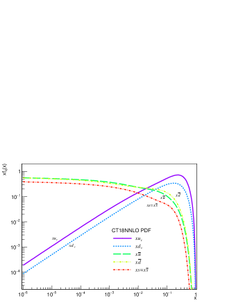
where . We require , , , , , , and , following CT18. The distribution of the gluon is ignored in this test, since it would complicate the PDF analysis to add gluon contributions in the pseudo data. The charm quark is also ignored because it is highly correlated with the gluon. Therefore, we have 24 free parameters in total. Their central values are also set to the best fit of CT18NNLO at the initial energy scale GeV [2], as listed in Tab. 1. Figure 1 depicts for different quarks. We note that in this study, these pseudo PDFs will not be evolved to a high energy scale relevant to the pseudo data introduced below. These pseudo PDFs do not resemble any of the CT18 PDF sets. They are merely designed to simplify our discussions on the effect of the second-order derivatives in Eq. (1) on the estimates of PDF-induced uncertainties.
| 3.385 (fixed) | 0.490 (fixed) | 0.414 | 0.414 | 0.288 | |
| 0.763 | 0.763 | -0.022 | -0.022 | -0.022 | |
| 3.036 | 3.036 | 7.737 | 7.737 | 10.31 | |
| 1.502 | 2.615 | 4 (fixed) | 4 (fixed) | 4(fixed) | |
| -0.147 | 1.828 | 0.618 | 0.292 | 0.466 | |
| 1.671 | 2.721 | 0.195 | 0.647 | 0.466 | |
| - | - | 0.871 | 0.474 | 0.225 | |
| - | - | 0.267 | 0.741 | 0.225 | |
| - | - | 0.733 | 1 (fixed) | 1 (fixed) |
A group of pseudo observables are also constructed according to the PDFs in Eq. (III) and Eq. (III). These observables, with uncertainties assigned, will be used as the data input in the pseudo global analysis. First, we introduce and :
| (18) |
as pseudo observables similar to the cross section measurements of the photon-exchange DIS process , and the -exchange DIS process . The functions are taken from Eq. (III) and Eq. (III), with values from Tab. 1. The coefficient 0.25 (1.2) roughly reflects the strength difference between the down-type and up-type quarks coupling to (). Note that we take the definitions of and , so that the and terms have a coefficient of 2. For simplicity, we ignore other contributions in a real calculation of the DIS process, such as the evolution of PDFs as a function of , the electroweak couplings and the higher order corrections. Although these effects would significantly change the predictions on any physical observable, the main sensitivity to the particular parton information in those observables remains. For , 28 data points are calculated, with 0.0001, 0.0002, 0.0003, 0.0004, 0.0005, 0.0006, 0.0007, 0.0008, 0.0009, 0.001, 0.002, 0.003, 0.004, 0.005, 0.006, 0.007, 0.008, 0.009, 0.01, 0.02, 0.03, 0.04, 0.05, 0.06, 0.07, 0.08, 0.09, 0.1. For , 16 points are calculated, with 0.01, 0.02, 0.03, 0.04, 0.05, 0.06, 0.07, 0.08, 0.09, 0.1, 0.15, 0.2, 0.25, 0.3, 0.35, 0.4.
Similarly, we introduce the following cross section observables in the proton-proton collisions: , and as:
| (19) | |||||
They approximately represent the vector boson productions of and . The momentum fractions and of the two initial quarks are connected by
where , and are the invariant mass, transverse momentum and rapidity of the bosons, respectively. In this work, is set to 90 GeV, which is near the pole of the and boson masses. Compared to , the transverse momentum of the single vector boson production is usually small. Therefore is ignored in this work. is set to 13 TeV. To gain information for different values, the cross section observables are calculated with different values of 0.1, 0.3, 0.5, 0.7, 0.9, 1.1, 1.3, 1.5, 1.7, 1.9, 2.1, 2.4, 2.8, 3.2, 4.0. The corresponding values range from 0.0001 to 0.38. In summary, 149 pseudo data points are introduced, corresponding to the DIS and Drell-Yan processes that are actually used in the PDF global analysis. For each data point, we assign a relative uncertainty of . This is a precision comparable to the HERA measurements and the LHC Drell-Yan measurements. For experimental results other than HERA and LHC, such as earlier DIS and semi-inclusive DIS measurements, their precisions are much lower. The experiments actually used in the PDF global analysis are summarized in Ref. [2]. Although these pseudo observables are only rough estimations rather than real calculations, they reflect the complexcity of using multiple data inputs to determine the PDF shape parameters.
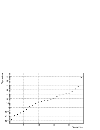
With the constructed PDFs, the pseudo observables and the assigned uncertainty, the Hessian matrix can be calculated accordingly. Since there are 24 free parameters in this test, the same number of eigenvectors and corresponding eigenvalues are acquired by diagonalizing the Hessian matrix. The eigenvalues in this test are shown in Fig. 2. As explained in Ref. [1], the eigenvalues in logarithmic scale rank as a line, reflecting the sensitivities of the input data. An eigenvector with large eigenvalue usually indicates that the information related to this eigenvector is well constrained by the input data. Otherwise, the input data has poor sensitivity to this eigenvector, leading to a small eigenvalue. Although data points in this analysis are much more than the free parameters being determined and the assigned uncertainty of is quite small, there is still some PDF information for certain regions and parton flavors, for which no pseudo observable gives good sensitivity. Therefore, some eigenvalues are small compared to others. This also happens in a real PDF global analysis [2, 3, 7].
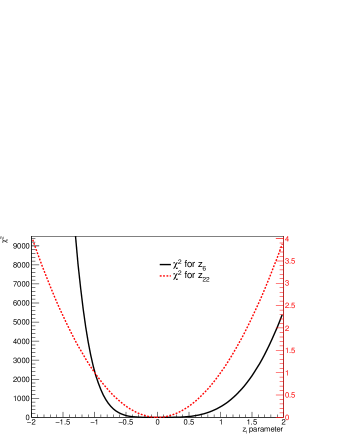
A simple test can numerically show whether the data inputs in a global fit provide a strong constraint to a particular eigenvector, as to be illustrated below. Once the Hessian matrix is diagonalized and the orthogonal displacements are acquired, one can look into the - relationship. Usually, if the eigenvector represented by is well constrained, is expected to be an ideal quadratic function of , giving for . In Fig. 3, the - relationship for and are shown and compared, as an example. For , the eigenvector has an eigenvalue at , thus its - relationship follows a good quadratic approximation. For however, the eigenvalue is at , resulting in a non-symmetric - relationship. When the eigenvalue is small, the normalization factor in Eq. (II) is enlarged. Therefore, any bias, such as inaccuracy in numerical calculations, would be significantly amplified. As a result, does not always yield , especially for those poorly constrained eigenvectors. In conclusion, when the - relationship does not follow a good quadratic approximation, the 1 standard deviation cannot be represented by . Therefore, in this work, the one standard deviation in the uncertainty estimation of an observable is calculated with the value which yields .
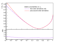
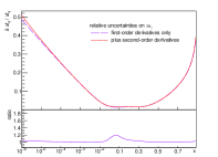
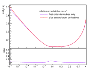
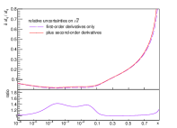
Following the method described in the previous section, the first-order and second-order PDF error sets are acquired according to Eq. (9) and Eq. (11), respectively. The uncertainty of any physical observable can be estimated accordingly. To numerically study the difference between the original Hessian method and the improved Hessian method, we compare the relative uncertainties on for , , , and , which are shown in Fig. 4. The improved Hessian method uncertainties, in which the second-order terms are included, are in general larger than the first-order calculations. Furthermore, the difference between the two uncertainties generally increases in the small and large region where the PDF uncertainty is larger. However, due to the complexity of the mixture of the parton information in multiple experimental observables, the uncertainties contributed from the second-order terms can still be relatively sizable, as compared to the first-order terms, even when the PDF uncertainty is small, i.e. when the PDFs are better constrained.
IV Pseudo global analysis with new data
The eigenvectors in a global analysis are determined from a particular set of data inputs. Therefore, both the first-order and second-order uncertainty estimations depend on the eigenvectors. To further test the improved Hessian method when the eigenvectors change, we introduce new experimental observables into the global fit, which are the new proton structure parameters and factorized from the forward-backward asymmetry of the Drell-Yan process [8], and the boost asymmetry in the diboson process [9]. These asymmetry variables were recently proposed at hadron colliders which can provide unique information on the proton structure. The and parameters factorize the proton structure information in and events. The two light quark initial states can be decoupled because the electroweak couplings of -- and -- are different. As a result, and separately provide the and quark information, which are mixed and indistinguishable in the measurement of the total cross section . is the asymmetry defined in the diboson production [9]. For example, in the process, the boson predominantly couples to the quark while the photon couples to the quark. Consequently, the boost asymmetry has a positive large value, namely is more boosted than the boson, because the initial state parton lunminosity is larger than for , etc. Therefore, the relative asymmetry between the initial states and (), which arises from the nature of the valence and sea quark differences, can be measured by comparing the energy or rapidity of the two bosons.
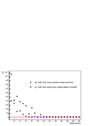
To gain information on the -dependence of the PDFs, the above pseudo observables are calculated with the values the same as the previous settings. The relative uncertainty of each data point is also assigned as . We repeat the calculations of the Hessian matrix now, using both the cross section observables and the new asymmetry observables; so we acquire the eigenvectors, eigenvalues, and the new orthogonal parameters accordingly. The new eigenvalues are shown in Fig. 5. With more data constraints introduced, the eigenvalues are in general larger. In Fig. 6, is shown both in the previous pseudo global fit and the new fit. As discussed, indicates a good quadratic approximation, so that the corresponding eigenvector is well constrained by data. Therefore, more eigenvectors have or close to 1 in the new global fit, as expected.

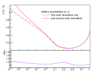
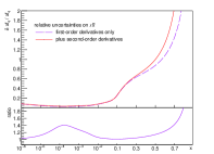
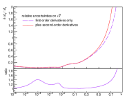
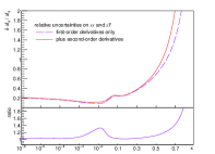
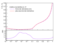
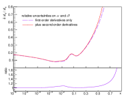
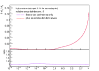
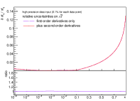
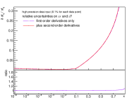
The relative uncertainties on for , , , and are shown in Fig. 7. As the constraints from the input data are strengthened, the estimated uncertainties are reduced with respect to the previous global fit in Fig. 4. In principle, when the uncertainties of individual eigenvectors decrease, the second-order uncertainties in Eq. (1) become less important with respect to the first-order ones. In Appendix B, we give another pseudo global fit in which the relative uncertainty of each data point is reduced to . With such a high precision, there is indeed no difference between the first-order and second-order calculation, as expected. In the present section, although the new asymmetry observables provide stronger constraints, their precisions are not high enough to reduce the second-order terms to a negligible level. The ratios between the first-order and second-order uncertainties in Fig. 7 can become even larger than the previous global fit in Fig. 4, due to the complexity of the multiple data fit. This reflects the fact that the uncertainty estimation in a PDF global fit depends highly on the data inputs. Therefore, the second-order calculation is not only a necessary procedure to get a better uncertainty estimation, but also a sufficient way to evaluate the power of the data constraints in a global fit. When the difference between the first-order and second-order uncertainties is small, it indicates a strong data constraint so that the output PDF is less dependent on various assumptions and the choice of non-perturbative functions.
V Conclusion
In this work, we propose an improved Hessian method in the PDF global analysis, which estimates the uncertainty with the inclusion of the complete set of second-order derivatives. A numerical test has been designed, in which a set of PDFs with multiple parameters are fitted to pseudo experimental observables. The test shows that when the precision of the input data used in a global analysis is limited, the improved Hessian method would give different uncertainties compared to the original method. Since the difference in the uncertainty can be reduced as the data constraints become stronger, one can tell whether a PDF global analysis is experimentally well constrained and less model-dependent, by comparing the uncertainties of the two methods.
VI Acknowledgement
Acknowledgements.
This work was supported by the National Natural Science Foundation of China under Grant No. 11721505, 11875245, 12061141005 and 12105275, and supported by the “USTC Research Funds of the Double First-Class Initiative”. This work was also supported by the U. S. National Science Foundation under Grant No. PHY-2310291.Appendix A Appendix A: PDF-induced uncertainty on physical observables
| (21) |
The standard deviation of can be calculated as:
| (22) | |||||
where and corresponds to the standard deviation and mathematical expectation. Note that , and for the gaussian distribution . Therefore, we have
| (23) |
Similarly, the standard deviation of is:
| (24) |
Given the fact that the and terms are uncorrelated since they contain independent gaussian distributions, the standard deviation of is simply the sum of and , which are positive values. Consequently, the inclusion of second-order derivative terms always increases the size of the PDF-induced uncertainty in the physical observable. Furthermore, including only the second-order diagonal terms generally underestimates the uncertainty.
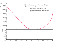
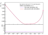
Appendix B Appendix B: A pseudo global fit with high precision data
A pseudo global fit with high precision data is performed in this section. 9 data variables are used, including , , , , , , , and . For each data point corresponding to a particular value, the relative uncertainty is set to . With sych high precision data used in the global fit, the uncertainty of the second-order derivative calculation is consistent with the first-order calculation. The result is shown in Fig. 8.
References
- [1] J. Pumplin, D. Stump, R. Brock, D. Casey, J. Huston, and J. Kalk, Phys. Rev. D 65, 014013 (2001).
- [2] Tie-Jiun Hou, Jun Gao, T. J. Hobbs et al., Phys. Rev. D 103, 014013 (2021).
- [3] S. Bailey, T. Cridge, L. A. Harland-Lang, A. D. Martin, R. S. Thorne, Eur. Phys. J. C 81, 341 (2021).
- [4] Carl Schmidt, Jon Pumplin, and C.-P. Yuan, Phys. Rev. D 98 094005 (2018).
- [5] Sayipjamal Dulat, Tie-Jiun Hou, Jun Gao et al., Phys. Rev. D 93, 033006 (2016).
- [6] Kari J. Eskola, Petja Paakkinen, Hannu Paukkunen, Eur. Phys. J. C 79, 511 (2019).
- [7] H. Abramowicz et al. (H1 and ZEUS) Collaborations, Eur. Phys. J. C 75, 580 (2015).
- [8] Siqi Yang, Yao Fu, Minghui Liu, Liang Han, Tie-Jiun Hou and C.-P. Yuan, Phys. Rev. D 106, 033001 (2022).
- [9] Siqi Yang, Mingzhe Xie, Yao Fu, Zihan Zhao, Minghui Liu, Liang Han, Tie-Jiun Hou and C. P.-Yuan, Phys. Rev. D 106, L051301 (2022).