Mathematical modeling and analysis for the chemotactic diffusion in porous media with incompressible Navier-Stokes equations over bounded domain

Fugui Ma1, Wenyi Tian3,777Author to whom any correspondence should be addressed. and Weihua Deng1,2 1 School of Mathematics and Statistics, Lanzhou University, Lanzhou 730000, China 2 State Key Laboratory of Natural Product Chemistry, Lanzhou University, Lanzhou 730000, China 3 Center for Applied Mathematics and KL-AAGDM, Tianjin University, Tianjin 300072, China mafg17@lzu.edu.cn, twymath@gmail.com and dengwh@lzu.edu.cn
Abstract

Myxobacteria aggregate and generate fruiting bodies in the soil to survive under starvation conditions. Considering soil as a porous medium, the biological mechanism and dynamic behavior of myxobacteria and slime (chemoattractants) affected by favorable environments in the soil can not be well characterized by the classical full parabolic Keller-Segel system combined with the incompressible Navier-Stokes equations. In this work, we employ the continuous time random walk (CTRW) approach to characterize the diffusion behavior of myxobacteria and slime in porous media at the microscale, and develop a new macroscopic model named as the time-fractional Keller-Segel system. Then it is coupled with the incompressible Navier-Stokes equations through transport and buoyancy, resulting in the TF-KSNS system, which reveals the biological mechanism from micro to macro and then appropriately describes the dynamic behavior of the chemotactic diffusion of myxobacteria and slime in the soil. In addition, we demonstrate that the TF-KSNS system associated with initial and no-flux/no-flux/Dirichlet boundary conditions over smoothly bounded domain in $\mathbb{R}^{d}$ ($d\geq 2$) admits a local well-posed mild solution, which continuously depends on the initial data with proper regularity under a small initial condition. Moreover, the blow-up of the mild solution is rigorously investigated.

Keywords: chemotactic diffusion, Keller-Segel system, Navier-Stokes equations, CTRW, mild solution, blow-up

AMS subject classifications: 35Q92, 35Q35, 35R11, 35A01, 35A02, 35B44

  • November 2024

1 Introduction

In this paper, we consider to discuss the mathematical modeling, local well-posedness analysis, and blow-up of the solution to the following time-fractional fully parabolic Keller-Segel (K-S) system coupled with the incompressible Navier-Stokes (N-S) equations (abbreviated to TF-KSNS)

$\displaystyle\partial^{\alpha}_{t}n+(\mathbf{u}\cdot\nabla)n=\Delta n-\nabla\cdot\left(n\chi(c)\nabla c\right),$ $\displaystyle x\in\Omega,~{}~{}0<t\leq T,$ (1.1a)
$\displaystyle\partial^{\alpha}_{t}c+(\mathbf{u}\cdot\nabla)c=\Delta c-\gamma c+n,$ $\displaystyle x\in\Omega,~{}~{}0<t\leq T,$ (1.1b)
$\displaystyle\partial_{t}\mathbf{u}+(\mathbf{u}\cdot\nabla)\mathbf{u}=\Delta\mathbf{u}-\nabla P+n\nabla\Phi,\quad\nabla\cdot\mathbf{u}=0,$ $\displaystyle x\in\Omega,~{}~{}0<t\leq T,$ (1.1c)

in a given convex, bounded and simply connected domain $\Omega\subseteq\mathbb{R}^{d}$ ($d\geq 2$) with smooth boundary, supplemented with no-flux boundary conditions for $n$ and $c$, a no-slip boundary condition for $\mathbf{u}$,

$$\frac{\partial n}{\partial\nu}=\frac{\partial c}{\partial\nu}=0,~{}~{}{\rm and}~{}~{}\mathbf{u}=0,\quad x\in\partial\Omega,~{}~{}0<t\leq T,$$ (1.2)

and the initial values

$$n(x,0)=n_{0}(x),~{}c(x,0)=c_{0}(x),~{}\mathbf{u}(x,0)=\mathbf{u}_{0}(x),\quad x\in\Omega,$$ (1.3)

where the unknown functions $n=n(x,t)$, $c=c(x,t)$, $\mathbf{u}=[u_{1}(x,t),\cdots,u_{d}(x,t)]^{T}$ and $P=P(x,t)$ denote the population density of myxobacteria, the slime concentration, the fluid velocity field, and the pressure, respectively; $\nu$ is the outer normal direction; the parameter function $\chi(c)$ measures the chemotactic sensitivity, which may depend on slime concentration $c$; $\gamma\geq 0$ represents the consumption rate of the slime; and $\Phi$ is the gravitational potential function. $\frac{\partial}{\partial\nu}$ denotes the outward normal derivative along the direction $\nu$ on $\partial\Omega$; the operator $\partial^{\alpha}_{t}$ is the Caputo fractional derivative defined by

โˆ‚tฮฑฮทโ€‹(โ‹…,t)=1ฮ“โ€‹(1โˆ’ฮฑ)โ€‹โˆซ0t(tโˆ’s)โˆ’ฮฑโ€‹โˆ‚sฮทโ€‹(โ‹…,s)โ€‹dโ€‹s,t>0,ฮฑโˆˆ(0,1).formulae-sequencesubscriptsuperscript๐›ผ๐‘ก๐œ‚โ‹…๐‘ก1ฮ“1๐›ผsuperscriptsubscript0๐‘กsuperscript๐‘ก๐‘ ๐›ผsubscript๐‘ ๐œ‚โ‹…๐‘ ๐‘‘๐‘ formulae-sequence๐‘ก0๐›ผ01\partial^{\alpha}_{t}\eta(\cdot,t)=\frac{1}{\Gamma(1-\alpha)}\int_{0}^{t}(t-s)^{-\alpha}\partial_{s}\eta(\cdot,s)ds,\quad t>0,~{}~{}\alpha\in(0,1). (1.4)

Typically, as $\alpha\rightarrow 1$, $\partial^{\alpha}_{t}$ turns out to be the first-order local differential operator $\partial_{t}$, and then the problem (1.1) reduces to the classical Keller-Segel system coupled to the Navier-Stokes equations (see, e.g., [7, 47, 48, 49]). It is indicated in (1.1) that chemotaxis and fluid dynamics are coupled through two components: the transport of myxobacteria and chemoattractants by the fluid, represented by the terms $(\mathbf{u}\cdot\nabla)n$ and $(\mathbf{u}\cdot\nabla)c$; and the external force $n\nabla\Phi$ exerted on the fluid by the myxobacteria due to buoyancy.

1.1 Background and previous works

Chemotaxis refers to the directional migration of substances driven by concentration gradients, such phenomenon is widely occurring in nature, such as chemistry [34], medicine [24, 43], biology [1, 38, 42], and etc. The mechanism of chemotaxis in biological processes has always been one of the main concerns of experimental scientists [11, 21, 46]. Although there are numerous different environmental settings in which bacterial chemotaxis has been observed, the majority of our understanding of this phenomenon comes from laboratory research on model organisms. Subsequently, the field on mathematical modeling of chemotaxis has grown to a wide range of topics, including system modeling, mechanistic basis, and mathematical analysis of the underlying equations.

Traditionally, macroscopic diffusion is defined as the spatiotemporal distribution of a population density of random walkers [5]. At the macroscopic level, Keller and Segel [28] built the well-known Keller-Segel model

$$\left\{\begin{aligned} &\partial_{t}n=D_{n}\Delta n-\nabla\cdot(n\chi(c)\nabla c),&&x\in\Omega,~{}~{}0<t\leq T,\\ &\partial_{t}c=D_{c}\Delta c-\gamma c+n,&&x\in\Omega,~{}~{}0<t\leq T,\end{aligned}\right.$$ (1.5)

where the positive constants $D_{n}$ and $D_{c}$ are the diffusivity of cells and chemoattractant, respectively. The term $\chi(c)=1/c$ represents the chemotactic sensitivity of the cells; more specifically, it expresses the tendency of the cells to aggregate due to the difference of concentration in the chemoattractant $c$. This mathematical model successfully describes chemotactic aggregation of cellular slime molds because of its intuitive simplicity, analytical tractability, and capacity to replicate key behaviors of chemotactic populations [22]. It has become the prevailing model for representing chemotactic dynamics in biological systems on the population level (see, e.g., [10, 22, 31, 39, 44]). This model has solutions blowing up for large enough initial conditions in dimensions $d\geq 2$, but the solutions are all regular in one dimension, which is confirmed with the patterns in the biological systems (see, e.g., [12, 50, 48]).

However, the model (1.5) ignores the interaction between the bacteria, chemoattractants, and the environment from the viewpoint of biology. Actually, the migration of bacteria is substantially affected by changes in the environment. For instance, Tuval et al. [46] proposed the following chemotaxis-Navier-Stokes model to describe pattern formation in populations of aerobic bacteria interacting with the liquid environment via transport and buoyancy

$$\left\{\begin{aligned} &\partial_{t}n+(\mathbf{u}\cdot\nabla)n=\Delta n-\nabla\cdot(n\chi(c)\nabla c),\quad&&x\in\Omega,~{}0<t\leq T,\\ &\partial_{t}c+(\mathbf{u}\cdot\nabla)c=\Delta c-nf(c),\quad&&x\in\Omega,~{}0<t\leq T,\\ &\partial_{t}\mathbf{u}+(\mathbf{u}\cdot\nabla)\mathbf{u}=\Delta\mathbf{u}+\nabla P+n\nabla\Phi,\quad\nabla\cdot\mathbf{u}=0,\quad&&x\in\Omega,~{}0<t\leq T.\end{aligned}\right.$$ (1.6)

Due to buoyancy, the bacteria exert force $n\nabla\Phi$ on the fluid, and the source term $n\nabla\Phi$ reflects that the fluctuations in bacterial population density cause forced changes in fluid velocity $\mathbf{u}$ and pressure $P$ with the given gravitational potential $\Phi$. In the chemotactic movement, bacteria migrate to areas with higher concentrations of chemoattractants, both bacteria and chemoattractants are transported by the surrounding fluid. Wang [47] considered a modified Keller-Segel system coupled with the Navier-Stokes fluid (i.e., the KSNS system) in a bounded domain $\Omega\subset\mathbb{R}^{3}$, where the terms $\chi(c)$ and $-nf(c)$ are replaced by $\chi(x,n,c)$ and $-c+n$, respectively. Under the condition $|\chi(x,n,c)|\leq C(1+n)^{-\alpha}$ with $\alpha>\frac{1}{3}$, the author proved the existence of global weak solutions of (1.6). Recently, Winkler [49] took into account the KSNS system with $\chi(c)=1$ and $-nf(c)=-c+n$ in a bounded domain $\Omega\subset\mathbb{R}^{2}$, equipped with the boundary conditions (1.2) and appropriate initial data. The corresponding initial-boundary value problem was testified to admit a globally defined generalized solution. One can also refer to [7, 48] and the references therein for more discussions.

In recent years, the Keller-Segel model with anomalous diffusion has gained popularity in [2, 13, 18, 32], etc. The time-fractional Keller-Segel system [2, 13] reads:

$$\left\{\begin{aligned} &\partial^{\alpha}_{t}n=D_{n}\Delta n-\nabla\cdot(n\chi(c)\nabla c),&&x\in\Omega,~{}~{}0<t\leq T,\\ &\partial^{\alpha}_{t}c=D_{c}\Delta c-\gamma c+n,&&x\in\Omega,~{}~{}0<t\leq T.\end{aligned}\right.$$ (1.7)

Azevedo et al. [2] proved an existence result of the time-fractional Keller-Segel system (1.7) with small initial data in a class of Besov-Morrey spaces in $\mathbb{R}^{d}$, $d\geq 2$. In [13], Costa and the co-authors dealt with local existence and blow-up of the solution to the time-fractional Keller-Segel system (1.7) in the setting of Lebesgue and Besov spaces for chemotaxis under homogeneous Neumann boundary conditions in a smooth domain of $\mathbb{R}^{d}$, $d\geq 2$. Moreover, the Keller-Segel system (1.7) was extended by Escudero in [18] to the space fractional Keller-Segel system, where the dispersal is characterized by the fractional Laplacian $(-\Delta)^{\alpha/2}$ with $\alpha\in(0,2)$. Li et al. [33] further investigated the Cauchy problems for the nonlinear fractional time-space generalized Keller-Segel system. Besides that, the time-space fractional Keller-Segel system was coupled with the incompressible Navier-Stokes equations by Jiang et al. [25, 26, 27], where the corresponding Cauchy initial problem was investigated, including the well-posedness, time decay, as well as asymptotic stability of its mild solution in the Lebesgue or Besov-Morrey spaces in $\mathbb{R}^{d}$, $d\geq 2$.

The time-fractional Keller-Segel system (1.7) in most existing literatures was simply obtained with the first-order derivative in (1.5) replaced by a time-fractional analogue. However, the physical and biological explanation of (1.7) describing the chemotactic diffusion combining anomalous diffusion still remains insufficient despite the efforts made in [32] and [5], let alone its coupled system with incompressible Navier-Stokes equations. To the best of our knowledge, anomalous diffusion models in the previous works were considered in static medium, such as time-fractional Fokker-Planck equations [29], time-fractional forward or backward Feynman-Kac equations [14, 16], time-fractional mobile-immobile equations [35], and etc. Nevertheless, many more biological processes, physical processes, and chemical reactions are occurring in the non-static medium; at the same time, the corresponding phenomena bring new inspirations and challenges in the modeling, analysis and simulations. Obviously, in our model (1.1), a non-static liquid field is described by the incompressible Navier-Stokes equations, which is the environment involving the chemotactic diffusion in the porous media. Moreover, the time-fractional Caputo derivative $\partial^{\alpha}_{t}$ in (1.1a)-(1.1b) is an integral-differential and non-local operator with historical memory. Therefore, the techniques for analyzing traditional Keller-Segel systems with the first-order time derivative, as well as the existing existence and regularity results, can not be directly generalized to the non-local analogue (1.1a)-(1.1b), which poses significant challenges for analysis. Another challenge comes from the handling of bilinear terms $(\mathbf{u}\cdot\nabla)n$ and $(\mathbf{u}\cdot\nabla)c$ in (1.1). Whenever the time-fractional Keller-Segel system is coupled with the incompressible Navier-Stokes equations, the analytical challenge would be even bigger for the investigations of well-posedness and blow-up of the solution. Thus, it is necessary to fill this gap for the TF-KSNS system (1.1).

1.2 Major contributions

Taking into account the distinctive advantages of the aforementioned works, the main contributions of the present work consist of two aspects.

The first one is to mathematically derive the model (1.1) for describing the chemotactic diffusion with anomalous diffusion in porous media; it provides reasonable mathematical and physical explanations of the biological process governed by the model. Specifically, the chemotactic diffusion of myxobacteria from a microscopic perspective in porous media can be characterized by the stochastic process with a power-law distribution of waiting time based on the continuous time random walk (CTRW), then the time-fractional Keller-Segel system is naturally derived into the mathematical model. In addition, at the microlevel, the sliding and diffusion of myxobacteria and slime (chemoattractants) in the soil are influenced by the surrounding environment in specific biological processes, such as liquid flow fields and rainwater present in the soil. Similar to the modeling of (1.6), we will also strongly couple the derived time-fractional Keller-Segel system with the incompressible Navier-Stokes equations describing the liquid flow fields and thus obtain the TF-KSNS system (1.1).

The other one is to perform a complete local well-posedness analysis of the TF-KSNS system (1.1) and to address the blow-up of its mild solution over a bounded domain $\Omega\subset\mathbb{R}^{d}$ ($d\geq 2$) with smooth boundary. To begin with, a complete metric space is first constructed, in which a map is simultaneously designed according to the expression of the mild solution, and it is verified that the map satisfies the conditions of the Banach fixed point theorem. Furthermore, the continuous dependence of the mild solution on the initial values is proved, and the asymptotic property of the mild solution is also discussed. We also prove the uniqueness of the continuous extension of the mild solution. Meanwhile, the blow-up of the solution is also analyzed by using the method of contradiction.

1.3 Outline of the paper

The paper is arranged as follows. In Section 2, we build the mathematical modeling of the TF-KSNS system (1.1) from microscopic to macroscopic under certain fundamental assumptions. Section 3 presents the key mathematical analysis results, including the local well-posedness and finite time blow-up of the mild solution to the TF-KSNS system (1.1)-(1.3). The detailed analyses of the two results are provided in Sections 4 and 5, respectively. Some conclusions are finally drawn in Section 6.

2 Mathematical modeling: From microscopic to macroscopic

2.1 The biology

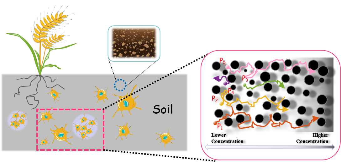
It is ubiquitous in environments that myxobacteria aggregate and eventually form fruiting bodies under starvation conditions (see, e.g., [17, 44]), new slimes are produced to help myxobacteria survive. Sliding myxobacteria employ chemotaxis to find chemical hotspots, which are high concentration areas of myxobacteria [6], we can refer to Fig. 1 for an intuitive understanding of the motility and directivity of myxobacteria. In order to get a deeper grasp of the biological mechanisms of myxobacteria chemotaxis, Steven [44] constructed a stochastic cellular automaton, in which the author took into account the biological hypotheses that myxobacteria produce slime traces where they like to glide on.

It is mentioned in [1] that โ€œnatural soils are host to a high density and diversity of microorganisms, and even deep-earth porous rocks provide a habitat for active microbial communities.โ€ The transport and distribution of myxobacteria in the soil (porous media) remain unclear due to their disordered flow and associated chemical gradients. In the next subsection, we consider to provide a mathematical explanation for a specific biological scenario depicted in Fig. 1 that myxobacteria aggregate and form fruiting bodies to secrete large amounts of slime for survival in the soil and derive the corresponding mathematical model.

Refer to caption
Figure 1: Illustration of the biological environment and the chemotactic diffusion: the myxobacteria (i.e., $\{P_{j}\}_{j\geq 1,j\in\mathbb{N}_{0}}$) glide in a porous medium towards a relatively high concentration of chemical signals, where black round holes with different sizes refer to obstacles in porous media, and the shades of gray in the background indicate the concentration of the chemoattractant; the darker the color, the higher the concentration. Myxobacteria aggregate and form fruiting bodies that produce new slime for survival.

2.2 Time-fractional chemotaxis diffusion equations with space- and time-dependent forces

Based on the biological mechanisms revealed in the previous subsection, we will employ the theory of stochastic processes at the microscale and the continuous time random walk (CTRW) approach to derive the time-fractional Keller-Segel system that characterizes the chemotactic diffusion of myxobacteria and slime in the soil.

In [32], Langlands and Henry utilized the balance equation (2.2) to describe the chemotaxis and diffusion dynamics of myxobacteria, where a special transition probability density function was constructed based on slime concentration. To further uncover the biological mechanism, we adopt the transfer probability density function proposed by Steven [44], to derive a micro dynamic model applicable to the biological scenario specified in the previous subsection and derive the corresponding macroscopic governing equations by the Laplace transform. The detailed modeling and derivation process are as follows.

To model the chemotactic diffusion of myxobacteria, we denote the probability distribution $n(x,t)$ to represent the concentration of myxobacteria at time $t$ and location $x$. By using the generalized CTRW balance equation in [23, 32], it incorporates the intricate mechanisms of chemotaxis as

$\displaystyle n(x,t)=n(x,0)\Psi(t)+\int_{0}^{t}$ $\displaystyle\big{[}p_{r}(x-\delta x\rightarrow x,s)n(x-\delta x,s)$
$\displaystyle+p_{l}(x+\delta x\rightarrow x,s)n(x+\delta x,s)\big{]}\psi(t-s)ds,$ (2.1)

where $\psi(t)$ is the probability density function (PDF) of waiting time, and $\Psi(t)$ is called survival probability, i.e., the waiting time on a site exceeds $t$, defined by ฮจโ€‹(t):=โˆซtโˆžฯˆโ€‹(s)โ€‹๐‘‘s=1โˆ’โˆซ0tฯˆโ€‹(s)โ€‹๐‘‘sassignฮจ๐‘กsuperscriptsubscript๐‘ก๐œ“๐‘ differential-d๐‘ 1superscriptsubscript0๐‘ก๐œ“๐‘ differential-d๐‘ \Psi(t):=\int_{t}^{\infty}\psi(s)ds=1-\int_{0}^{t}\psi(s)ds. In (2.2), $p_{r}(x-\delta x\rightarrow x,t)$ and $p_{l}(x+\delta x\rightarrow x,t)$ are the transition probabilities of jumping from the adjacent grid points ($x\pm\delta x$) in the right and left directions to $x$, respectively. When different distribution functions $\psi(t)$, $p_{r}(x,t)$, and $p_{l}(x,t)$ are selected in (2.2), we will observe different chemotaxis and diffusion dynamics of myxobacteria. Therefore, it is crucial to pick appropriate distribution functions $\psi(t)$, $p_{r}(x,t)$ and $p_{l}(x,t)$ for accurately describing the chemotaxis and diffusion process of myxobacteria.

As is well known, the sub-diffusion process has an advantage for describing the diffusion-transport process of particles in porous media. Inspired by this and taking into account the sliding trace of myxobacteria and the hindrance of narrow gaps in the soil to myxobacteria migration, we take a power law PDF of waiting time as

$$\psi(t)\sim\tau^{\alpha}/t^{1+\alpha},\quad 0<\alpha<1,$$ (2.2)

for $t\gg\tau$, where $\tau$ is a characteristic waiting time scale [23, 32]. Taking inspiration from the work of Stevens [44, (8) and (9)], the transition probability law governing jumps to the left or right direction in (2.2) is determined by the relative concentration of the slime (chemoattractant) on either side of the current location, as follows

$$\left\{\begin{aligned} p_{l}(x\rightarrow x-\delta x,t)&=\frac{v(x-\delta x,t)}{v(x-\delta x,t)+v(x+\delta x,t)},\\ p_{r}(x\rightarrow x+\delta x,t)&=\frac{v(x+\delta x,t)}{v(x-\delta x,t)+v(x+\delta x,t)},\end{aligned}\right.$$ (2.3)

where $v:=g(c)$ depends on the density (concentration) of the slime (chemoattractant) at time $t$ and point $x$, $g$ is a given function. The transition probability in (2.3) indicates that myxobacteria are attracted by chemoattractants from different directions, which is reasonable in the biological mechanism.

Next, we are ready to derive the governing equations for modeling the chemotaxis and diffusion process of myxobacteria and slime in the soil. Employing the Laplace transform to the balance equation (2.2) and the relationship $\hat{\Psi}(z)=z^{-1}(1-\hat{\psi}(z))$, we can obtain the discrete space evolution equation

$\displaystyle z\hat{n}(x,z)-\hat{n}(x,0)=\frac{\hat{\psi}(z)}{\hat{\Psi}(z)}\big{\{}-\hat{n}(x,z)$ $\displaystyle+\mathcal{L}_{t\rightarrow z}\{p_{r}(x-\delta x\rightarrow x,t)n(x-\delta x,t)\}(z)$ (2.4)
$\displaystyle+\mathcal{L}_{t\rightarrow z}\{p_{l}(x+\delta x\rightarrow x,t)n(x+\delta x,t)\}(z)\big{\}},$

where the notation โ€œw^โ€‹(z)^๐‘ค๐‘ง\hat{w}(z)โ€ represents the Laplace transform of the function $v(t)$ with respect to the time variable $t$, which is also denoted as $\hat{w}(z):=\mathcal{L}_{t\rightarrow z}\{w(t)\}(z)$. According to (2.2) and $\hat{\Psi}(z)=z^{-1}(1-\hat{\psi}(z))$, it obtains that

$$\frac{\hat{\psi}(z)}{\hat{\Psi}(z)}\sim D_{\alpha}\frac{z^{1-\alpha}}{\tau^{\alpha}},\quad{\rm with}\quad D_{\alpha}=\frac{\alpha}{\Gamma(1-\alpha)}.$$ (2.5)

Then it derives from (2.5) and the inverse Laplace transform of (2.4) that

$\displaystyle\frac{dn(x,t)}{dt}=\frac{D_{\alpha}}{\tau^{\alpha}}\frac{d^{\alpha-1}}{dt^{\alpha-1}}\big{\{}-n(x,t)$ $\displaystyle+p_{r}(x-\delta x\rightarrow x,t)n(x-\delta x,t)$
$\displaystyle+p_{l}(x+\delta x\rightarrow x,t)n(x+\delta x,t)\big{\}},$ (2.6)

where it employs the property of the Laplace transform of the Riemann-Liouville fractional derivative ($\mathcal{L}_{t\rightarrow z}\big{\{}\frac{d^{\alpha}}{dt^{\alpha}}w(t)\big{\}}(z)=z^{\alpha}\hat{w}(z)-\frac{d^{\alpha-1}}{dt^{\alpha-1}}w(t)\big{|}_{t=0},~{}0<\alpha<1$) and the vanishing behavior near the lower terminal ($\frac{d^{\alpha-1}}{dt^{\alpha-1}}w(t)|_{t=0}=0$, [40, P100-P105]).

Subsequently, we consider the continuous limit of the aforementioned spatially discrete formulation (2.2) with $\delta x\rightarrow 0$. To this end, we utilize (2.3) and the Taylor expansions of the lattice functions at the point $x$ up to and including terms of order $(\delta x)^{2}$. It yields from (2.3) the following expression:

$\displaystyle-n(x,t)+p_{r}(x-\delta x\rightarrow x,t)n(x-\delta x,t)+p_{l}(x+\delta x\rightarrow x,t)n(x+\delta x,t)$
$\displaystyle=\frac{c(x,t)}{c(x,t)+c(x-2\delta x)}n(x-\delta x,t)+\frac{c(x,t)}{c(x,t)+c(x+2\delta x)}n(x+\delta x,t)-n(x,t)$
$\displaystyle=\frac{v(x,t)\big{[}\big{(}v(x,t)+v(x+2\delta x,t)\big{)}n(x-\delta x,t)+\big{(}v(x,t)+v(x-2\delta x,t)\big{)}n(x+\delta x,t)\big{]}}{\big{(}v(x,t)+v(x-2\delta x,t)\big{)}\big{(}v(x,t)+v(x+2\delta x,t)\big{)}}$
$\displaystyle~{}~{}~{}~{}-\frac{n(x,t)\big{(}v(x,t)+v(x-2\delta x,t)\big{)}\big{(}v(x,t)+v(x+2\delta x,t)\big{)}}{\big{(}v(x,t)+v(x-2\delta x,t)\big{)}\big{(}v(x,t)+v(x+2\delta x,t)\big{)}}.$

In addition, with simple calculations, it holds that

$\displaystyle\frac{1}{\big{(}v(x,t)+v(x-2\delta_{x},t)\big{)}\big{(}v(x,t)+v(x+2\delta x,t)\big{)}}\approx\frac{1}{4v^{2}(x,t)},\quad{\rm as}~{}~{}\delta x\rightarrow 0,$
$\displaystyle v(x,t)\big{[}\big{(}v(x,t)+v(x+2\delta x,t)\big{)}n(x-\delta x,t)+\big{(}v(x,t)+v(x-2\delta x,t)\big{)}n(x+\delta x,t)\big{]}$
$\displaystyle\approx 4v(x,t)\Big{(}v(x,t)n(x,t)+\frac{1}{2}(\delta x)^{2}v(x,t)\partial_{xx}n(x,t)$
$\displaystyle\hskip 62.59596pt-(\delta x)^{2}\partial_{x}v(x,t)\partial_{x}n(x,t)+(\delta x)^{2}n(x,t)\partial_{xx}v(x,t)\Big{)},$

and

$\displaystyle n(x,t)\big{(}v(x,t)+v(x-2\delta x,t)\big{)}\big{(}v(x,t)+v(x+2\delta x,t)\big{)}$
$\displaystyle\approx 4n(x,t)(v(x,t))^{2}+8n(x,t)(\delta x)^{2}v(x,t)\partial_{xx}v(x,t)-4(\delta x)^{2}n(x,t)\big{(}\partial_{x}v(x,t)\big{)}^{2}.$

Then, the above results deduce that

$$\frac{dn(x,t)}{dt}=\frac{d^{\alpha-1}}{dt^{\alpha-1}}\Big{\{}\mathcal{D}_{\alpha}\partial_{xx}n(x,t)-\mathcal{T}_{\alpha}\partial_{x}\Big{(}\frac{n(x,t)}{v(x,t)}\partial_{x}v(x,t)\Big{)}\Big{\}},$$ (2.7)

where $\mathcal{D}_{\alpha}=\frac{D_{\alpha}(\delta x)^{2}}{2\tau^{\alpha}}$ and $\mathcal{T}_{\alpha}=\frac{D_{\alpha}(\delta x)^{2}}{\tau^{\alpha}}$ as $\delta x,\tau\rightarrow 0$. Thus, by using $v=g(c)$ and the connection between Riemann-Liouville and Caputo fractional derivatives (see [40]), it leads to

$$\partial_{t}^{\alpha}n(x,t)=\mathcal{D}_{\alpha}\partial_{xx}n(x,t)-\mathcal{T}_{\alpha}\partial_{x}\big{(}n(x,t)\chi(c)\partial_{x}v(x,t)\big{)},$$ (2.8)

where $\chi(c)=g^{\prime}(c)/g(c)$. For $v(x,t)=c(x,t)$ in (2.3), it refers to the model with $\chi(c)=1/c$ in [8, 22]; for $v(x,t)=e^{\beta c(x,t)}$, it covers the model with $\chi(c)\equiv\beta$ in [8, 32]. Upon selecting suitable coefficients, we obtain the equation (1.1a) including the transport term $(\mathbf{u}\cdot\nabla)n$ by virtue of the fluid velocity. Obviously, as $\alpha\rightarrow 1^{+}$, (2.8) reduces to the first equation in the classical Keller-Segel system (1.5).

As we know, the diffusion of particles (slime molecules) in porous media (soil) can be precisely described by the subdiffusion equation [36], i.e., $\partial_{t}^{\alpha}c(x,t)=\Delta c(x,t)$. Meanwhile, the slime in the soil will continuously dry up and deplete over time, and the aggregation of myxobacteria can create new slime. As a result, the reaction and source term $-\gamma c(x,t)+n(x,t)$, characterizing the decay of slime and new generation of slime, are merged into the subdiffusion equation together with the transport term $(\mathbf{u}\cdot\nabla)c$. Then it produces (1.1b) to explain the diffusion mechanism of chemoattractants (slime) in the soil (porous media).

Analogous to the derivation of the system (1.6) from (1.5), we also strongly couple (1.1a) and (1.1b) with the well-known incompressible Navier-Stokes equations (1.1c) to accurately characterize the biological processes and the living environment, where the migration and chemotaxis of myxobacteria and slime under space- and time-dependent forces are driven by the fluid flow in the soil.

3 Main results

This section presents the analysis results for the TF-KSNS system (1.1) with the no-flux/no-flux/Dirichlet boundary conditions (1.2) in smoothly bounded domain and the initial data in (1.3). Under some assumptions on the initial values, the problem admits a unique local mild solution; the blow-up and asymptotic behaviors of the mild solution are also established.

3.1 Preliminaries

We denote $L^{p}(\Omega)$ ($p\geq 1$) as the standard Lebesgue space and $W^{m,p}(\Omega)$ the Sobolev space. In order to analyze the well-posedness and regularity of (1.1)-(1.3) as precisely as possible, we need some $L^{p}$-$L^{q}$ estimates of the heat semigroup $e^{t\Delta}$ under the homogenous Neumann and Dirichlet boundary conditions in Lemmas 3.1 and 3.2, respectively.

Lemma 3.1 ([10, 50]).

Let $(e^{t\Delta})_{t\geq 0}$ be the heat semigroup under the homogenous Neumann boundary condition. Then there exist some positive constants $C_{i}$ depending on $\Omega$, $p$ and $q$ such that the following estimates hold.

  1. (i)

    If $2\leq p<\infty$, for all $t>0$ and $\omega\in W^{1,p}(\Omega)$, then

    $$\big{\|}\nabla e^{t\Delta}\omega\big{\|}_{L^{p}(\Omega)}\leq C_{1}\|\nabla\omega\|_{L^{p}(\Omega)}.$$ (3.1)
  2. (ii)

    If $1\leq p\leq q\leq\infty$, for all $t>0$ and $\omega\in L^{p}(\Omega)$, then

    $$\big{\|}e^{t\Delta}\omega\big{\|}_{L^{q}(\Omega)}\leq C_{2}\big{(}1+t^{-\frac{d}{2}(\frac{1}{p}-\frac{1}{q})}\big{)}\|\omega\|_{L^{p}(\Omega)}.$$ (3.2)
  3. (iii)

    If $1\leq p\leq q\leq\infty$, for all $t>0$ and $\omega\in L^{p}(\Omega)$, then

    $$\big{\|}\nabla e^{t\Delta}\omega\big{\|}_{L^{q}(\Omega)}\leq C_{3}\big{(}1+t^{-\frac{1}{2}-\frac{d}{2}(\frac{1}{p}-\frac{1}{q})}\big{)}\|\omega\|_{L^{p}(\Omega)}.$$ (3.3)
  4. (iv)

    If $1<p\leq q\leq\infty$, for all $t>0$ and $\omega\in L^{p}(\Omega;\mathbb{R}^{d})$, then

    $$\big{\|}e^{t\Delta}\nabla\cdot\omega\big{\|}_{L^{q}(\Omega)}\leq C_{4}\big{(}1+t^{-\frac{1}{2}-\frac{d}{2}(\frac{1}{p}-\frac{1}{q})}\big{)}\|\omega\|_{L^{p}(\Omega)}.$$ (3.4)

For the heat semigroup $(e^{t\Delta})_{t\geq 0}$ with the homogenous Dirichlet boundary condition, it also has the analogous results to the Neumann boundary case.

Lemma 3.2.

Let $\Omega\in\mathbb{R}^{d}$ ($d\geq 2$) be a domain of class $C^{1,1}$, and $\{e^{t\Delta}\}_{t\geq 0}$ the Dirichlet heat semigroup in $\Omega$.

  1. (i)

    For $1\leq p\leq q\leq\infty$ and all $\omega\in L^{p}(\Omega)$, it holds

    $$\|e^{t\Delta}\omega\|_{L^{q}(\Omega)}\leq C_{1}t^{-\frac{d}{2}(\frac{1}{p}-\frac{1}{q})}\|\omega\|_{L^{p}(\Omega)},~{}~{}\forall~{}t>0.$$ (3.5)
  2. (ii)

    For $1\leq p\leq q\leq\infty$ and all $\omega\in L^{p}(\Omega)$, it holds

    $$\|\nabla e^{t\Delta}\omega\|_{L^{q}(\Omega)}\leq C_{2}\big{(}1+t^{-\frac{1}{2}-\frac{d}{2}(\frac{1}{p}-\frac{1}{q})}\big{)}\|\omega\|_{L^{p}(\Omega)},~{}~{}\forall~{}t>0.$$ (3.6)
  3. (iii)

    For $1\leq p\leq q\leq\infty$ and all $\omega\in L^{p}(\Omega;\mathbb{R}^{d})$, it holds

    $$\|e^{t\Delta}\nabla\cdot\omega\|_{L^{q}(\Omega)}\leq C_{3}\big{(}1+t^{-\frac{1}{2}-\frac{d}{2}(\frac{1}{p}-\frac{1}{q})}\big{)}\|\omega\|_{L^{p}(\Omega)},~{}~{}\forall~{}t>0.$$ (3.7)
Proof.

Regarding (i), the estimate (3.5) is a better-known result in [41, Proposition 48.4]. As for (ii), (3.6) can be derived by the heat kernel estimate in [30] and Youngโ€™s inequality for convolution.

Now we turn to prove (iii). By [9, Corollary 1.4], there holds

$$\big{\|}e^{t\Delta}\nabla\cdot\omega\big{\|}_{L^{q}(\Omega)}=\sup_{\begin{subarray}{c}\phi\in L^{q^{*}}(\Omega)\\ \|\phi\|_{L^{q^{*}}(\Omega)}\leq 1\end{subarray}}\Big{|}\int_{\Omega}e^{t\Delta}\nabla\cdot\omega\phi\Big{|}=\max_{\begin{subarray}{c}\phi\in L^{q^{*}}(\Omega)\\ \|\phi\|_{L^{q^{*}}(\Omega)}\leq 1\end{subarray}}\Big{|}\int_{\Omega}e^{t\Delta}\nabla\cdot\omega\phi\Big{|}.$$ (3.8)

Note that $e^{t\Delta}$ is a self-adjoint operator. Then, by an analogous approach in the proof of Lemma 1.3 (iv) in [50], for any $\phi\in C_{0}^{\infty}(\Omega)$, integrating by parts and employing (3.6) with $1\leq q\leq p<\infty$ obtains that

$\displaystyle\Big{|}\int_{\Omega}e^{t\Delta}\nabla\cdot\omega\phi\Big{|}$ $\displaystyle\leq\Big{|}-\int_{\Omega}\omega\cdot\nabla e^{t\Delta}\phi\Big{|}\leq\|\omega\|_{L^{p}}\big{\|}\nabla e^{t\Delta}\phi\big{\|}_{L^{p*}}$
$\displaystyle\leq C\big{(}1+t^{-\frac{1}{2}-\frac{d}{2}(\frac{1}{q^{*}}-\frac{1}{p*})}\big{)}\|\omega\|_{L^{p}(\Omega)}\|\phi\|_{L^{q^{*}}(\Omega)},$ (3.9)

where $\frac{1}{p}+\frac{1}{p*}=1$, $\frac{1}{q}+\frac{1}{q*}=1$, and $\frac{1}{q^{*}}-\frac{1}{p*}=\frac{1}{p}-\frac{1}{q}$. Since $C_{0}^{\infty}(\Omega)$ is dense in $L^{p}(\Omega)$ for any $1\leq p<+\infty$ [9, Corollary 4.23], then we derive from (3.8) and (3.1) that the estimate (3.7) holds for $1\leq p\leq q<\infty$. Furthermore, for the case $q=p=\infty$, by choosing $\omega\in(C_{0}^{\infty})^{d}$ as in [15, Lemma 2.1] and taking $1\leq\tilde{q}<p=\infty$, we have from (3.5) that

$\displaystyle\big{\|}e^{t\Delta}\nabla\cdot\omega\big{\|}_{L^{\infty}(\Omega)}$ $\displaystyle=\big{\|}e^{\frac{t}{2}\Delta}\big{(}e^{\frac{t}{2}\Delta}\nabla\cdot\omega\big{)}\big{\|}_{L^{\infty}(\Omega)}\leq C\big{(}1+t^{-\frac{1}{2}-\frac{d}{2\tilde{q}}}\big{)}\|\omega\|_{L^{\tilde{q}}(\Omega)}.$

As $\Omega$ being a smooth and bounded domain, therefore, taking the limit $\tilde{q}\rightarrow\infty$, we can obtain $\|e^{t\Delta}\nabla\cdot\omega\|_{L^{\infty}(\Omega)}\leq c(1+t^{-\frac{1}{2}})\|\omega\|_{L^{\infty}(\Omega)}$. The proof is completed. โˆŽ

Let $\kappa>-1$, $\lambda\in\mathbb{C}$, the Wright function [40] is defined by the complex convergent series $W_{\kappa,\lambda}(z):=\sum_{j=0}^{\infty}\frac{z^{j}}{j!\Gamma(\kappa j+\lambda)},~{}z\in\mathbb{C},$ where $\Gamma(\cdot)$ is the Euler-Gamma function. The Mainardi function denoted as $M_{\alpha}(z)$ is a specific case of the Wright function and given by $M_{\alpha}(z):=W_{-\alpha,1-\alpha}(-z)$. Following [2], it has been proved that $M_{\alpha}$ is non-negative and satisfies

$$\int_{0}^{\infty}t^{\gamma}M_{\alpha}(t)dt=\frac{\Gamma(1+\gamma)}{\Gamma(1+\alpha\gamma)},\quad~{}\gamma>-1.$$ (3.10)

The third one is the Mittag-Leffler function defined by $E_{\alpha,\beta}(z):=\sum_{j=0}^{\infty}\frac{z^{j}}{\Gamma(\alpha j+\beta)}$, and $E_{\alpha}(z):=E_{\alpha,1}(z),~{}z\in\mathbb{C}.$ The Mainardi function $M_{\alpha}(z)$ and the Mittag-Leffler function $E_{\alpha,\beta}(z)$ satisfy the following properties (see, e.g., [13, 3])

$$\left\{\begin{aligned} &E_{\alpha}(t^{\alpha}\Delta)=\int_{0}^{\infty}M_{\alpha}(s)e^{st^{\alpha}\Delta}ds,\\ &E_{\alpha,\alpha}(t^{\alpha}\Delta)=\int_{0}^{\infty}\alpha sM_{\alpha}(s)e^{st^{\alpha}\Delta}ds,\end{aligned}\right.$$ (3.11)
$$\left\{\begin{aligned} &E_{\alpha}\left(t^{\alpha}(\Delta-\gamma)\right)=\int_{0}^{\infty}M_{\alpha}(s)H_{\gamma}(st^{\alpha})ds,\\ &E_{\alpha,\alpha}\left(t^{\alpha}(\Delta-\gamma)\right)=\int_{0}^{\infty}\alpha sM_{\alpha}(s)H_{\gamma}(st^{\alpha})ds,\end{aligned}\right.$$ (3.12)

where $H_{\gamma}(t):=e^{t(\Delta-\gamma)}:L^{p}(\Omega)\rightarrow L^{q}(\Omega)$ is the damped heat semigroup with $\gamma>0$.

The Mittag-Leffler functions involving the Laplacian, called Mittag-Leffler operators, play a central role to represent the mild solution in (4.1) and satisfy some important properties in the following lemmas.

Lemma 3.3 (Strong continuity [3, 13]).

The families $(E_{\alpha}(t^{\alpha}\Delta))_{t\geq 0}$, $(E_{\alpha}(t^{\alpha}(\Delta-\gamma)))_{t\geq 0}$, $(E_{\alpha,\alpha}(t^{\alpha}\Delta))_{t\geq 0}$, and $(E_{\alpha,\alpha}(t^{\alpha}(\Delta-\gamma)))_{t\geq 0}$ are strongly continuous with respect to variable $t$ in $L^{q}(\Omega)$ with $1\leq q<\infty$.

Based on the $L^{p}$-$L^{q}$ estimates for the Neumann heat semigroup in Lemma 3.1, we have the following estimates of the Mittag-Leffler operators.

Lemma 3.4.

Let $E_{\alpha}(t^{\alpha}\Delta)$, $E_{\alpha}(t^{\alpha}(\Delta-\gamma))$, $E_{\alpha,\alpha}(t^{\alpha}\Delta)$ and $E_{\alpha,\alpha}(t^{\alpha}(\Delta-\gamma))$ be defined by (3.11)-(3.12). For $t>0$, $\rho>2$ and $1\leq q\leq\infty$, there exists a constant $C>0$ only depending on $\Omega$, $\alpha$, $d$ and $q$, such that the following estimates hold:

$\displaystyle\big{\|}E_{\alpha}(t^{\alpha}\Delta)\big{\|}_{L^{q}(\Omega)\rightarrow L^{q}(\Omega)}\leq C,$ (3.13)
$\displaystyle\big{\|}E_{\alpha,\alpha}(t^{\alpha}(\Delta-\gamma))\big{\|}_{L^{q}(\Omega)\rightarrow L^{q}(\Omega)}\leq C,$ (3.14)
$\displaystyle\big{\|}E_{\alpha,\alpha}(t^{\alpha}(\Delta-\gamma))\big{\|}_{L^{\frac{\rho q}{\rho+1}}(\Omega)\rightarrow L^{\rho q}(\Omega)}\leq C(1+t^{-\frac{\alpha d}{2q}}),~{}~{}q>d,$ (3.15)
$\displaystyle\big{\|}\nabla E_{\alpha,\alpha}(t^{\alpha}(\Delta-\gamma))\big{\|}_{L^{q}(\Omega)\rightarrow L^{q}(\Omega)}\leq C(1+t^{-\frac{\alpha}{2}}),$ (3.16)
$\displaystyle\big{\|}\nabla E_{\alpha,\alpha}(t^{\alpha}(\Delta-\gamma))\big{\|}_{L^{\frac{\rho q}{\rho+1}}(\Omega)\rightarrow L^{\rho q}(\Omega)}\leq C(1+t^{-\frac{\alpha}{2}-\frac{\alpha d}{2q}}),~{}~{}q>d,$ (3.17)
$\displaystyle\big{\|}E_{\alpha,\alpha}(t^{\alpha}\Delta)\nabla\cdot\big{\|}_{L^{\rho q}(\Omega)\rightarrow L^{\rho q}(\Omega)}\leq C(1+t^{-\frac{\alpha}{2}}),$ (3.18)
$\displaystyle\big{\|}E_{\alpha,\alpha}(t^{\alpha}\Delta)\nabla\cdot\big{\|}_{L^{\frac{\rho q}{\rho+1}}(\Omega)\rightarrow L^{\rho q}(\Omega)}\leq C(1+t^{-\frac{\alpha}{2}-\frac{\alpha d}{2q}}),~{}~{}q>d.$ (3.19)
Proof.

The estimates (3.14), (3.16) and (3.18) were precisely proved in [13, Lemma 3.3] by using the estimates of the heat semigroup under Neumann boundary conditions in Lemma 3.1. We next consider to derive the others. Specifically, (3.2) in Lemma 3.1 and (3.10) imply (3.13) as follows

$\displaystyle\left\|E_{\alpha}(t^{\alpha}\Delta)\omega\right\|_{L^{q}(\Omega)}$ โ‰คโˆซ0โˆžMฮฑโ€‹(s)โ€‹โ€–esโ€‹tฮฑโ€‹ฮ”โ€‹ฯ‰โ€–Lqโ€‹(ฮฉ)โ€‹๐‘‘sabsentsuperscriptsubscript0subscript๐‘€๐›ผ๐‘ subscriptnormsuperscript๐‘’๐‘ superscript๐‘ก๐›ผฮ”๐œ”superscript๐ฟ๐‘žฮฉdifferential-d๐‘ \displaystyle\leq\int_{0}^{\infty}M_{\alpha}(s)\left\|e^{st^{\alpha}\Delta}\omega\right\|_{L^{q}(\Omega)}ds
โ‰คโˆซ0โˆžMฮฑโ€‹(s)โ€‹(1+C2)โ€‹๐‘‘sโ€‹โ€–ฯ‰โ€–Lqโ€‹(ฮฉ)โ‰คCโ€‹โ€–ฯ‰โ€–Lqโ€‹(ฮฉ).absentsuperscriptsubscript0subscript๐‘€๐›ผ๐‘ 1subscript๐ถ2differential-d๐‘ subscriptnorm๐œ”superscript๐ฟ๐‘žฮฉ๐ถsubscriptnorm๐œ”superscript๐ฟ๐‘žฮฉ\displaystyle\leq\int_{0}^{\infty}M_{\alpha}(s)\left(1+C_{2}\right)ds\|\omega\|_{L^{q}(\Omega)}\leq C\|\omega\|_{L^{q}(\Omega)}.

Regarding (3.15), applying (3.2) in Lemma 3.1, we have

$\displaystyle\left\|E_{\alpha,\alpha}(t^{\alpha}(\Delta-\gamma))\omega\right\|_{L^{\rho q}(\Omega)}$ โ‰คโˆซ0โˆžฮฑโ€‹sโ€‹Mฮฑโ€‹(s)โ€‹eโˆ’ฮณโ€‹sโ€‹tฮฑโ€‹โ€–esโ€‹tฮฑโ€‹ฮ”โ€‹ฯ‰โ€–Lฯโ€‹qโ€‹(ฮฉ)โ€‹๐‘‘sabsentsuperscriptsubscript0๐›ผ๐‘ subscript๐‘€๐›ผ๐‘ superscript๐‘’๐›พ๐‘ superscript๐‘ก๐›ผsubscriptnormsuperscript๐‘’๐‘ superscript๐‘ก๐›ผฮ”๐œ”superscript๐ฟ๐œŒ๐‘žฮฉdifferential-d๐‘ \displaystyle\leq\int_{0}^{\infty}\alpha sM_{\alpha}(s)e^{-\gamma st^{\alpha}}\big{\|}e^{st^{\alpha}\Delta}\omega\big{\|}_{L^{\rho q}(\Omega)}ds
โ‰คC2โ€‹โˆซ0โˆžฮฑโ€‹sโ€‹Mฮฑโ€‹(s)โ€‹(1+(sโ€‹tฮฑ)โˆ’d2โ€‹q)โ€‹โ€–ฯ‰โ€–Lฯโ€‹qฯ+1โ€‹(ฮฉ)โ€‹๐‘‘sabsentsubscript๐ถ2superscriptsubscript0๐›ผ๐‘ subscript๐‘€๐›ผ๐‘ 1superscript๐‘ superscript๐‘ก๐›ผ๐‘‘2๐‘žsubscriptnorm๐œ”superscript๐ฟ๐œŒ๐‘ž๐œŒ1ฮฉdifferential-d๐‘ \displaystyle\leq C_{2}\int_{0}^{\infty}\alpha sM_{\alpha}(s)\big{(}1+(st^{\alpha})^{-\frac{d}{2q}}\big{)}\|\omega\|_{L^{\frac{\rho q}{\rho+1}}(\Omega)}ds
$\displaystyle\leq C_{2}\alpha\Big{(}\frac{1}{\Gamma(1+\alpha)}+t^{-\frac{\alpha d}{2q}}\frac{\Gamma(2-\frac{d}{2q})}{\Gamma(1+\alpha(1-\frac{d}{2q}))}\Big{)}\|\omega\|_{L^{\frac{\rho q}{\rho+1}}(\Omega)}$
$\displaystyle\leq C(1+t^{-\frac{\alpha d}{2q}})\|\omega\|_{L^{\frac{\rho q}{\rho+1}}(\Omega)}.$

By the similar approach, (3.17) and (3.19) can be derived by (3.3) and (3.4) in Lemma 3.1, respectively. โˆŽ

3.2 Main results

In this subsection, we present the main results on the local existence, uniqueness, and blow-up of the mild solution to the TF-KSNS system (1.1)-(1.3) with the chemotactic sensitivity being $\chi(c)=1$. To begin with, the following assumptions are made similar to those for (1.6) in [47, 49].

Assumption 3.1.

Let $q>2d$, $\rho\geq 2$ and $\beta=\frac{\alpha d}{2\rho q}$ throughout the paper, and the following two conditions hold.

  1. (i)

    The time-independent gravitational potential parameter function $\Phi$ satisfies $\Phi\in W^{1,\infty}(\Omega);$

  2. (ii)

    The initial data $(n_{0},c_{0},\mathbf{u}_{0})$ fulfills that: $n_{0}\in L^{\infty}(\Omega)$ is nonnegative with $n_{0}\not\equiv 0$, $c_{0}\in W^{1,\infty}(\Omega)$ is nonnegative and $\mathbf{u}_{0}\in D(\mathcal{A})$.

In Assumption 3.1 (ii), $D(\mathcal{A}):=W^{2,q}(\Omega;\mathbb{R}^{d})\cap W_{0}^{1,q}(\Omega;\mathbb{R}^{d})\cap L^{q}_{\sigma}(\Omega;\mathbb{R}^{d})$ denotes the domain of the Stokes operator $\mathcal{A}:=-\mathcal{P}\Delta$ in the space $L^{q}_{\sigma}(\Omega;\mathbb{R}^{d})$ with $L^{q}_{\sigma}(\Omega;\mathbb{R}^{d}):=\{\phi\in L^{q}(\Omega;\mathbb{R}^{d}):\nabla\cdot\phi=0\}$ being the subspace of all solenoidal vector fields in $L^{q}(\Omega;\mathbb{R}^{d})$, and $\mathcal{P}$ is the Helmholtz projection operator [37, 45] from $L^{q}(\Omega;\mathbb{R}^{d})$ into $L^{q}_{\sigma}(\Omega;\mathbb{R}^{d})$, which is introduced to remove the pressure term in (1.1c) and then obtain the solution representations (4.1). It holds that $\mathcal{P}[L^{q}(\Omega;\mathbb{R}^{d})]=L_{\sigma}^{q}(\Omega;\mathbb{R}^{d})$, and $\mathcal{P}$ is bounded in $L^{p}(\Omega)$ for smooth boundary $\partial\Omega$ and any $p\in(1,+\infty)$ [19, Theorem 1].

The local existence and uniqueness of the mild solution to (1.1)-(1.3) under the smallness conditions (4.3) and (4.7) are provided in the following theorem.

Theorem 3.1 (Well-posedness and $L^{q}$-regularity).

Let $\Omega\subset\mathbb{R}^{d}$ $(d\geq 2)$ be a bounded convex domain with a smooth boundary. If the conditions in Assumption 3.1 hold, then there exists $T>0$ such that the initial-boundary value problem (1.1)-(1.3) admits a unique mild solution $(n,c,\mathbf{u}):[0,T]\rightarrow L^{q}(\Omega;\mathbb{R}^{2+d})$ satisfying

$$n,c\in C([0,T],L^{q}(\Omega)),~{}\nabla c,\mathbf{u}\in C\big{(}[0,T],L^{q}(\Omega;\mathbb{R}^{d})\big{)},$$

and the following asymptotic property holds

$$t^{\beta}\|n(t)\|_{L^{q}(\Omega)}\rightarrow 0,\quad t^{\beta}\|c(t)\|_{L^{q}(\Omega)}\rightarrow 0,\quad t^{\beta}\|\mathbf{u}(t)\|_{L^{q}(\Omega)}\rightarrow 0,\quad{\rm as}~{}t\rightarrow 0^{+}.$$ (3.20)

Moreover, the solution $(n,c,\mathbf{u})$ is continuously dependent on the initial data $(n_{0},c_{0},\mathbf{u}_{0})$.

With Theorem 3.1, the result of blow-up of the mild solution to (1.1)-(1.3) can be further obtained, which is stated as follows.

Theorem 3.2 (Blow-up).

Under the same conditions in Theorem 3.1, the solution $(n,c,\mathbf{u})$ can be uniquely continued up to maximal time $T_{max}>T$ with Tmโ€‹aโ€‹x:=sup{T>0:(โ€‹1.1โ€‹)โˆ’(โ€‹1.3โ€‹)โ€‹hโ€‹aโ€‹sโ€‹aโ€‹uโ€‹nโ€‹iโ€‹qโ€‹uโ€‹eโ€‹sโ€‹oโ€‹lโ€‹uโ€‹tโ€‹iโ€‹oโ€‹nโ€‹(n,c,๐ฎ)โˆˆCโ€‹([0,T];Lฯโ€‹qโ€‹(ฮฉ;โ„2+d))}.assignsubscript๐‘‡๐‘š๐‘Ž๐‘ฅsupremumconditional-set๐‘‡0italic-(1.1italic-)italic-(1.3italic-)โ„Ž๐‘Ž๐‘ ๐‘Ž๐‘ข๐‘›๐‘–๐‘ž๐‘ข๐‘’๐‘ ๐‘œ๐‘™๐‘ข๐‘ก๐‘–๐‘œ๐‘›๐‘›๐‘๐ฎ๐ถ0๐‘‡superscript๐ฟ๐œŒ๐‘žฮฉsuperscriptโ„2๐‘‘T_{max}:=\sup\big{\{}T>0:\eqref{eq:problem}-\eqref{eq:InitialC}~{}{has~{}a~{}unique~{}solution}~{}(n,c,\mathbf{u})\in C([0,T];L^{\rho q}(\Omega;\mathbb{R}^{2+d}))\big{\}}. Moreover, if $T_{max}<+\infty$, then

$$\underset{t\rightarrow T^{-}_{max}}{\lim\sup}~{}\|n(t)\|_{L^{\rho q}(\Omega)}=+\infty,~{}\underset{t\rightarrow T^{-}_{max}}{\lim\sup}~{}\|c(t)\|_{L^{\rho q}(\Omega)}=+\infty,~{}\underset{t\rightarrow T^{-}_{max}}{\lim\sup}~{}\|\mathbf{u}(t)\|_{L^{\rho q}(\Omega)}=+\infty.$$

The proofs of Theorems 3.1 and 3.2 are rigorously established in Sections 4 and 5, respectively.

4 Analysis of local well-posedness and regularity

4.1 The mild solution of the TF-KSNS system

As $\mathcal{L}_{t\rightarrow z}\{E_{\alpha}(-t^{\beta}A)\}=z^{\beta}/(z^{\beta}+A)$ and $\mathcal{L}_{t\rightarrow z}\{t^{\beta-1}E_{\alpha,\beta}(-t^{\beta}A)\}=z^{\alpha-\beta}/(z^{\alpha}+A)$ [20], then taking the Laplace and inverse Laplace transform of the equations in system (1.1) with the projection of (1.1c) by the Helmholtz projection operator $\mathcal{P}$, it formally derives the following Duhamel-type integral equations

$$\left\{\small\begin{aligned} n(t)&=E_{\alpha}(t^{\alpha}\Delta)n_{0}-\int_{0}^{t}(t-s)^{\alpha-1}E_{\alpha,\alpha}\big{(}(t-s)^{\alpha}\Delta\big{)}\big{(}\mathbf{u}\cdot\nabla n+\nabla\cdot(n\nabla c)\big{)}(s)ds,\\ c(t)&=E_{\alpha}(t^{\alpha}(\Delta-\gamma))c_{0}-\int_{0}^{t}(t-s)^{\alpha-1}E_{\alpha,\alpha}\big{(}(t-s)^{\alpha}(\Delta-\gamma)\big{)}\big{(}\mathbf{u}\cdot\nabla c-n\big{)}(s)ds,\\ \mathbf{u}(t)&=e^{t\Delta}\mathbf{u}_{0}-\int_{0}^{t}e^{\Delta(t-s)}\mathcal{P}\big{(}\nabla\cdot(\mathbf{u}\otimes\mathbf{u})(s)-n(s)\nabla\Phi\big{)}ds,\end{aligned}\right.$$ (4.1)

where $\mathbf{u}\otimes\mathbf{u}=(u_{j}u_{k})_{j,k=1}^{d}$ with the notation โ€œโŠ—tensor-product\otimesโ€ being the usual tensor product, and $\nabla\cdot(\mathbf{u}\otimes\mathbf{u})=(\mathbf{u}\cdot\nabla)\mathbf{u}$ due to the incompressible condition $\nabla\cdot\mathbf{u}=0$. With (4.1), the definition of the mild solution to the TF-KSNS system (1.1)-(1.3) reads in the following.

Definition 4.1 ($L^{q}(\Omega)$-mild solution).

A triple of continuous functions $(n,c,\mathbf{u}):[0,T]\rightarrow L^{q}(\Omega;\mathbb{R}^{2+d})$ satisfying the Duhamel-type integral equations presented in (4.1), is called an $L^{q}(\Omega)$-mild solution to the TF-KSNS system (1.1)-(1.3).

4.2 The proof of Theorem 3.1

In light of the aforementioned preparations, in this section, we will employ the Banach fixed point theorem [9, Theorem 5.7] to demonstrate the local well-posedness of the mild solution in $L^{q}$ space to the TF-KSNS system (1.1) with the initial-boundary conditions (1.2)-(1.3) satisfying (4.3)-(4.7), as well as Assumption 3.1. To this end, we introduce a Banach space given by

$$\mathbb{S}_{T}:=\big{\{}(n,c,\mathbf{u})\mid n\in\mathcal{X},c\in\mathcal{X},\nabla c\in\mathcal{X}^{d},\mathbf{u}\in\mathcal{X}^{d}\big{\}}$$

as the solution space, endowed with the norm

$\displaystyle\|(n,c,\mathbf{u})\|_{\mathbb{S}_{T}}:=$ $\displaystyle\sup_{t\in(0,T)}t^{\beta}\|n(t)\|_{L^{\rho q}(\Omega)}+\sup_{t\in(0,T)}t^{\beta}\|c(t)\|_{L^{\rho q}(\Omega)}$
$\displaystyle+\sup_{t\in(0,T)}t^{\beta}\|\nabla c(t)\|_{L^{\rho q}(\Omega)}+\sup_{t\in(0,T)}t^{\beta}\|\mathbf{u}(t)\|_{L^{\rho q}(\Omega)},$

where $\mathcal{X}$ is the Banach space

$$\mathcal{X}:=\Big{\{}v\in C((0,T];L^{\rho q}(\Omega))\mid\|v\|_{\mathcal{X}}:=\sup_{t\in(0,T)}t^{\beta}\|v(t)\|_{L^{\rho q}(\Omega)}<+\infty\Big{\}},$$

with $T\in(0,1)$ being small enough satisfying the conditions in (4.3)-(4.7).

We denote $\mathbb{X}$ a nonempty complete metric subspace of $\mathbb{S}_{T}$ indicated by

$$\mathbb{X}:=\big{\{}(n,c,\mathbf{u})\in\mathbb{S}_{T}\mid\|(n,c,\mathbf{u})\|_{\mathbb{S}_{T}}\leq 3R\big{\}},$$

then, given $t\in(0,T)$ with sufficiently small $T$, it provides a map $\mathcal{M}=(\mathcal{M}_{1},\mathcal{M}_{2},\mathcal{M}_{3})$ on $\mathbb{X}$ as follows

$$\left\{\small\begin{aligned} \mathcal{M}_{1}(n,c,\mathbf{u})&:=E_{\alpha}(t^{\alpha}\Delta)n_{0}-\int_{0}^{t}(t-s)^{\alpha-1}E_{\alpha,\alpha}\big{(}(t-s)^{\alpha}\Delta\big{)}\big{(}\mathbf{u}\cdot\nabla n+\nabla\cdot(n\nabla c)\big{)}(s)ds,\\ \mathcal{M}_{2}(n,c,\mathbf{u})&:=E_{\alpha}(t^{\alpha}(\Delta-\gamma))c_{0}-\int_{0}^{t}(t-s)^{\alpha-1}E_{\alpha,\alpha}\big{(}(t-s)^{\alpha}(\Delta-\gamma)\big{)}\big{(}\mathbf{u}\cdot\nabla c-n\big{)}(s)ds,\\ \mathcal{M}_{3}(n,c,\mathbf{u})&:=e^{t\Delta}\mathbf{u}_{0}-\int_{0}^{t}e^{(t-s)\Delta}\mathcal{P}\big{(}\nabla\cdot(\mathbf{u}\otimes\mathbf{u})(s)-n(s)\nabla\Phi\big{)}ds.\end{aligned}\right.$$ (4.2)

Additionally, we take $T>0$ being small enough to satisfy the following inequalities.

$\displaystyle T^{\beta}\|\nabla c_{0}\|_{L^{\rho q}(\Omega)}\leq\frac{R}{8C},$ (4.3)
$\displaystyle T^{\frac{\alpha}{2}}B(1-\beta,\frac{\alpha}{2})+CT^{\alpha}B(1-\beta,\alpha)+CT\leq\frac{1}{8},$ (4.4)
$\displaystyle T^{\frac{\alpha}{2}-\frac{\alpha d}{2q}-\beta}\leq\frac{1}{8CB(1-2\beta,\frac{\alpha}{2}-\frac{\alpha d}{2q})R},$ (4.5)
$\displaystyle T^{\frac{1}{2}-\frac{d}{2\rho q}-\beta}\leq\frac{1}{8CB(1-2\beta,\frac{1}{2}-\frac{d}{2\rho q})R},$ (4.6)
$\displaystyle\begin{aligned} \sup_{t\in(0,T)}t^{\beta}\left\|E_{\beta}(t^{\alpha}\Delta)n_{0}\right\|_{L^{\rho q}(\Omega)}+\sup_{t\in(0,T)}t^{\beta}\left\|E_{\beta}(t^{\alpha}(\Delta-\gamma))c_{0}\right\|_{L^{\rho q}(\Omega)}\\ +\sup_{t\in(0,T)}t^{\beta}\|e^{t\Delta}\mathbf{u}_{0}\|_{L^{\rho q}(\Omega)}\leq\frac{R}{8},\end{aligned}$ (4.7)

where (4.7) is reasonable from Lemmas 3.4, 3.2 and Assumption 3.1, and $B(\cdot,\cdot)$ is the beta function defined as Bโ€‹(a,b):=โˆซ01saโˆ’1โ€‹(1โˆ’s)bโˆ’1โ€‹๐‘‘sassign๐ต๐‘Ž๐‘superscriptsubscript01superscript๐‘ ๐‘Ž1superscript1๐‘ ๐‘1differential-d๐‘ B(a,b):=\int_{0}^{1}s^{a-1}(1-s)^{b-1}ds. Based on the aforementioned arrangements, we first derive a preliminary Lemma as follows.

Lemma 4.1 (Priori estimates in $L^{\rho q}(\Omega)$).

For $t\in(0,T)$, $n,c\in\mathcal{X}$, and $\mathbf{u},\mathbf{u}_{1},\mathbf{u}_{2}\in\mathcal{X}^{d}$, we have

I1:=โˆซ0t(tโˆ’s)ฮฑโˆ’1โ€‹โ€–Eฮฑ,ฮฑโ€‹((tโˆ’s)ฮฑโ€‹ฮ”)โ€‹(๐ฎโ‹…โˆ‡n)โ€‹(s)โ€–Lฯโ€‹qโ€‹๐‘‘sโ‰คCโ€‹tฮฑ2โˆ’ฮฑโ€‹d2โ€‹qโˆ’2โ€‹ฮฒโ€‹Bโ€‹(1โˆ’2โ€‹ฮฒ,ฮฑ2โˆ’ฮฑโ€‹d2โ€‹q)โ€‹โ€–nโ€–๐’ณโ€‹โ€–๐ฎโ€–๐’ณ,:subscript๐ผ1absentabsentsuperscriptsubscript0๐‘กsuperscript๐‘ก๐‘ ๐›ผ1subscriptnormsubscript๐ธ๐›ผ๐›ผsuperscript๐‘ก๐‘ ๐›ผฮ”โ‹…๐ฎโˆ‡๐‘›๐‘ superscript๐ฟ๐œŒ๐‘ždifferential-d๐‘ missing-subexpressionabsent๐ถsuperscript๐‘ก๐›ผ2๐›ผ๐‘‘2๐‘ž2๐›ฝ๐ต12๐›ฝ๐›ผ2๐›ผ๐‘‘2๐‘žsubscriptnorm๐‘›๐’ณsubscriptnorm๐ฎ๐’ณ\displaystyle\begin{aligned} I_{1}:&=\int_{0}^{t}(t-s)^{\alpha-1}\big{\|}E_{\alpha,\alpha}\big{(}(t-s)^{\alpha}\Delta\big{)}\big{(}\mathbf{u}\cdot\nabla n\big{)}(s)\big{\|}_{L^{\rho q}}ds\\ &\leq Ct^{\frac{\alpha}{2}-\frac{\alpha d}{2q}-2\beta}B(1-2\beta,\frac{\alpha}{2}-\frac{\alpha d}{2q})\|n\|_{\mathcal{X}}\|\mathbf{u}\|_{\mathcal{X}},\end{aligned} (4.8)
I2:=โˆซ0t(tโˆ’s)ฮฑโˆ’1โ€‹โ€–Eฮฑ,ฮฑโ€‹((tโˆ’s)ฮฑโ€‹ฮ”)โ€‹โˆ‡โ‹…(nโ€‹โˆ‡c)โ€‹(s)โ€–Lฯโ€‹qโ€‹๐‘‘sโ‰คCโ€‹tฮฑ2โˆ’ฮฑโ€‹d2โ€‹qโˆ’2โ€‹ฮฒโ€‹Bโ€‹(1โˆ’2โ€‹ฮฒ,ฮฑ2โˆ’ฮฑโ€‹d2โ€‹q)โ€‹โ€–nโ€–๐’ณโ€‹โ€–โˆ‡cโ€–๐’ณ,:subscript๐ผ2absentabsentsuperscriptsubscript0๐‘กsuperscript๐‘ก๐‘ ๐›ผ1subscriptnormโ‹…subscript๐ธ๐›ผ๐›ผsuperscript๐‘ก๐‘ ๐›ผฮ”โˆ‡๐‘›โˆ‡๐‘๐‘ superscript๐ฟ๐œŒ๐‘ždifferential-d๐‘ missing-subexpressionabsent๐ถsuperscript๐‘ก๐›ผ2๐›ผ๐‘‘2๐‘ž2๐›ฝ๐ต12๐›ฝ๐›ผ2๐›ผ๐‘‘2๐‘žsubscriptnorm๐‘›๐’ณsubscriptnormโˆ‡๐‘๐’ณ\displaystyle\begin{aligned} I_{2}:&=\int_{0}^{t}(t-s)^{\alpha-1}\big{\|}E_{\alpha,\alpha}\big{(}(t-s)^{\alpha}\Delta\big{)}\nabla\cdot\big{(}n\nabla c\big{)}(s)\big{\|}_{L^{\rho q}}ds\\ &\leq Ct^{\frac{\alpha}{2}-\frac{\alpha d}{2q}-2\beta}B(1-2\beta,\frac{\alpha}{2}-\frac{\alpha d}{2q})\|n\|_{\mathcal{X}}\|\nabla c\|_{\mathcal{X}},\end{aligned} (4.9)
I3:=โˆซ0t(tโˆ’s)ฮฑโˆ’1โ€‹โ€–Eฮฑ,ฮฑโ€‹((tโˆ’s)ฮฑโ€‹(ฮ”โˆ’ฮณ))โ€‹(๐ฎโ‹…โˆ‡c)โ€‹(s)โ€–Lฯโ€‹qโ€‹๐‘‘sโ‰คCโ€‹tฮฑโˆ’ฮฑโ€‹d2โ€‹qโˆ’2โ€‹ฮฒโ€‹Bโ€‹(1โˆ’2โ€‹ฮฒ,ฮฑโˆ’ฮฑโ€‹d2โ€‹q)โ€‹โ€–๐ฎโ€–๐’ณโ€‹โ€–โˆ‡cโ€–๐’ณ,:subscript๐ผ3absentabsentsuperscriptsubscript0๐‘กsuperscript๐‘ก๐‘ ๐›ผ1subscriptnormsubscript๐ธ๐›ผ๐›ผsuperscript๐‘ก๐‘ ๐›ผฮ”๐›พโ‹…๐ฎโˆ‡๐‘๐‘ superscript๐ฟ๐œŒ๐‘ždifferential-d๐‘ missing-subexpressionabsent๐ถsuperscript๐‘ก๐›ผ๐›ผ๐‘‘2๐‘ž2๐›ฝ๐ต12๐›ฝ๐›ผ๐›ผ๐‘‘2๐‘žsubscriptnorm๐ฎ๐’ณsubscriptnormโˆ‡๐‘๐’ณ\displaystyle\begin{aligned} I_{3}:&=\int_{0}^{t}(t-s)^{\alpha-1}\big{\|}E_{\alpha,\alpha}\big{(}(t-s)^{\alpha}(\Delta-\gamma)\big{)}\big{(}\mathbf{u}\cdot\nabla c\big{)}(s)\big{\|}_{L^{\rho q}}ds\\ &\leq Ct^{\alpha-\frac{\alpha d}{2q}-2\beta}B(1-2\beta,\alpha-\frac{\alpha d}{2q})\|\mathbf{u}\|_{\mathcal{X}}\|\nabla c\|_{\mathcal{X}},\end{aligned} (4.10)
I4:=โˆซ0t(tโˆ’s)ฮฑโˆ’1โ€‹โ€–Eฮฑ,ฮฑโ€‹((tโˆ’s)ฮฑโ€‹(ฮ”โˆ’ฮณ))โ€‹nโ€‹(s)โ€–Lฯโ€‹qโ€‹๐‘‘sโ‰คCโ€‹tฮฑโˆ’ฮฒโ€‹Bโ€‹(1โˆ’ฮฒ,ฮฑ)โ€‹โ€–nโ€–๐’ณ,:subscript๐ผ4absentabsentsuperscriptsubscript0๐‘กsuperscript๐‘ก๐‘ ๐›ผ1subscriptnormsubscript๐ธ๐›ผ๐›ผsuperscript๐‘ก๐‘ ๐›ผฮ”๐›พ๐‘›๐‘ superscript๐ฟ๐œŒ๐‘ždifferential-d๐‘ missing-subexpressionabsent๐ถsuperscript๐‘ก๐›ผ๐›ฝ๐ต1๐›ฝ๐›ผsubscriptnorm๐‘›๐’ณ\displaystyle\begin{aligned} I_{4}:&=\int_{0}^{t}(t-s)^{\alpha-1}\big{\|}E_{\alpha,\alpha}\big{(}(t-s)^{\alpha}(\Delta-\gamma)\big{)}n(s)\big{\|}_{L^{\rho q}}ds\\ &\leq Ct^{\alpha-\beta}B(1-\beta,\alpha)\|n\|_{\mathcal{X}},\end{aligned} (4.11)
I5:=โˆซ0t(tโˆ’s)ฮฑโˆ’1โ€‹โ€–โˆ‡Eฮฑ,ฮฑโ€‹((tโˆ’s)ฮฑโ€‹(ฮ”โˆ’ฮณ))โ€‹(๐ฎโ‹…โˆ‡c)โ€‹(s)โ€–Lฯโ€‹qโ€‹๐‘‘sโ‰คCโ€‹tฮฑ2โˆ’ฮฑโ€‹d2โ€‹qโˆ’2โ€‹ฮฒโ€‹Bโ€‹(1โˆ’2โ€‹ฮฒ,ฮฑ2โˆ’ฮฑโ€‹d2โ€‹q)โ€‹โ€–๐ฎโ€–๐’ณโ€‹โ€–โˆ‡cโ€–๐’ณ,:subscript๐ผ5absentabsentsuperscriptsubscript0๐‘กsuperscript๐‘ก๐‘ ๐›ผ1subscriptnormโˆ‡subscript๐ธ๐›ผ๐›ผsuperscript๐‘ก๐‘ ๐›ผฮ”๐›พโ‹…๐ฎโˆ‡๐‘๐‘ superscript๐ฟ๐œŒ๐‘ždifferential-d๐‘ missing-subexpressionabsent๐ถsuperscript๐‘ก๐›ผ2๐›ผ๐‘‘2๐‘ž2๐›ฝ๐ต12๐›ฝ๐›ผ2๐›ผ๐‘‘2๐‘žsubscriptnorm๐ฎ๐’ณsubscriptnormโˆ‡๐‘๐’ณ\displaystyle\begin{aligned} I_{5}:&=\int_{0}^{t}(t-s)^{\alpha-1}\big{\|}\nabla E_{\alpha,\alpha}\big{(}(t-s)^{\alpha}(\Delta-\gamma)\big{)}\big{(}\mathbf{u}\cdot\nabla c\big{)}(s)\big{\|}_{L^{\rho q}}ds\\ &\leq Ct^{\frac{\alpha}{2}-\frac{\alpha d}{2q}-2\beta}B(1-2\beta,\frac{\alpha}{2}-\frac{\alpha d}{2q})\|\mathbf{u}\|_{\mathcal{X}}\|\nabla c\|_{\mathcal{X}},\end{aligned} (4.12)
I6:=โˆซ0t(tโˆ’s)ฮฑโˆ’1โ€‹โ€–โˆ‡Eฮฑ,ฮฑโ€‹((tโˆ’s)ฮฑโ€‹(ฮ”โˆ’ฮณ))โ€‹nโ€‹(s)โ€–Lฯโ€‹qโ€‹๐‘‘sโ‰คCโ€‹tฮฑ2โˆ’ฮฒโ€‹Bโ€‹(1โˆ’ฮฒ,ฮฑ2)โ€‹โ€–nโ€–๐’ณ,:subscript๐ผ6absentabsentsuperscriptsubscript0๐‘กsuperscript๐‘ก๐‘ ๐›ผ1subscriptnormโˆ‡subscript๐ธ๐›ผ๐›ผsuperscript๐‘ก๐‘ ๐›ผฮ”๐›พ๐‘›๐‘ superscript๐ฟ๐œŒ๐‘ždifferential-d๐‘ missing-subexpressionabsent๐ถsuperscript๐‘ก๐›ผ2๐›ฝ๐ต1๐›ฝ๐›ผ2subscriptnorm๐‘›๐’ณ\displaystyle\begin{aligned} I_{6}:&=\int_{0}^{t}(t-s)^{\alpha-1}\big{\|}\nabla E_{\alpha,\alpha}\big{(}(t-s)^{\alpha}(\Delta-\gamma)\big{)}n(s)\big{\|}_{L^{\rho q}}ds\\ &\leq Ct^{\frac{\alpha}{2}-\beta}B(1-\beta,\frac{\alpha}{2})\|n\|_{\mathcal{X}},\end{aligned} (4.13)
I7:=โˆซ0tโ€–e(tโˆ’s)โ€‹ฮ”โ€‹๐’ซโ€‹(โˆ‡โ‹…(๐ฎ1โŠ—๐ฎ2)โ€‹(s))โ€–Lฯโ€‹qโ€‹๐‘‘sโ‰คCโ€‹t12โˆ’d2โ€‹ฯโ€‹qโˆ’2โ€‹ฮฒโ€‹Bโ€‹(1โˆ’2โ€‹ฮฒ,12โˆ’d2โ€‹ฯโ€‹q)โ€‹โ€–๐ฎ1โ€–๐’ณโ€‹โ€–๐ฎ2โ€–๐’ณ,:subscript๐ผ7absentabsentsuperscriptsubscript0๐‘กsubscriptnormsuperscript๐‘’๐‘ก๐‘ ฮ”๐’ซโ‹…โˆ‡tensor-productsubscript๐ฎ1subscript๐ฎ2๐‘ superscript๐ฟ๐œŒ๐‘ždifferential-d๐‘ missing-subexpressionabsent๐ถsuperscript๐‘ก12๐‘‘2๐œŒ๐‘ž2๐›ฝ๐ต12๐›ฝ12๐‘‘2๐œŒ๐‘žsubscriptnormsubscript๐ฎ1๐’ณsubscriptnormsubscript๐ฎ2๐’ณ\displaystyle\begin{aligned} I_{7}:&=\int_{0}^{t}\big{\|}e^{(t-s)\Delta}\mathcal{P}\big{(}\nabla\cdot(\mathbf{u}_{1}\otimes\mathbf{u}_{2})(s)\big{)}\big{\|}_{L^{\rho q}}ds\\ &\leq Ct^{\frac{1}{2}-\frac{d}{2\rho q}-2\beta}B(1-2\beta,\frac{1}{2}-\frac{d}{2\rho q})\|\mathbf{u}_{1}\|_{\mathcal{X}}\|\mathbf{u}_{2}\|_{\mathcal{X}},\end{aligned} (4.14)
I8:=โˆซ0tโ€–e(tโˆ’s)โ€‹ฮ”โ€‹๐’ซโ€‹(nโ€‹(s)โ€‹โˆ‡ฮฆ)โ€–Lฯโ€‹qโ€‹๐‘‘sโ‰คCโ€‹t1โˆ’ฮฒโ€‹โ€–nโ€–๐’ณ.assignsubscript๐ผ8superscriptsubscript0๐‘กsubscriptnormsuperscript๐‘’๐‘ก๐‘ ฮ”๐’ซ๐‘›๐‘ โˆ‡ฮฆsuperscript๐ฟ๐œŒ๐‘ždifferential-d๐‘ ๐ถsuperscript๐‘ก1๐›ฝsubscriptnorm๐‘›๐’ณ\displaystyle I_{8}:=\int_{0}^{t}\big{\|}e^{(t-s)\Delta}\mathcal{P}\big{(}n(s)\nabla\Phi\big{)}\big{\|}_{L^{\rho q}}ds\leq Ct^{1-\beta}\|n\|_{\mathcal{X}}. (4.15)
Proof.

As $\mathbf{u}\cdot\nabla n=\nabla\cdot(\mathbf{u}n)$ obtained by the incompressible condition $\nabla\cdot\mathbf{u}=0$, thanks to (3.19) in Lemma 3.4 and $L^{\rho q}(\Omega)\hookrightarrow L^{q}(\Omega)$ as $\rho q>q$, it derives that

$\displaystyle I_{1}$ โ‰คCโ€‹โˆซ0t(tโˆ’s)ฮฑ2โˆ’ฮฑโ€‹d2โ€‹qโˆ’1โ€‹โ€–(๐ฎโ€‹n)โ€‹(s)โ€–Lฯโ€‹qฯ+1โ€‹(ฮฉ)โ€‹๐‘‘sabsent๐ถsuperscriptsubscript0๐‘กsuperscript๐‘ก๐‘ ๐›ผ2๐›ผ๐‘‘2๐‘ž1subscriptnorm๐ฎ๐‘›๐‘ superscript๐ฟ๐œŒ๐‘ž๐œŒ1ฮฉdifferential-d๐‘ \displaystyle\leq C\int_{0}^{t}(t-s)^{\frac{\alpha}{2}-\frac{\alpha d}{2q}-1}\|(\mathbf{u}n)(s)\|_{L^{\frac{\rho q}{\rho+1}}(\Omega)}ds
โ‰คCโ€‹โˆซ0t(tโˆ’s)ฮฑ2โˆ’ฮฑโ€‹d2โ€‹qโˆ’1โ€‹โ€–nโ€‹(s)โ€–Lฯโ€‹qโ€‹(ฮฉ)โ€‹โ€–๐ฎโ€‹(s)โ€–Lqโ€‹(ฮฉ)โ€‹๐‘‘sabsent๐ถsuperscriptsubscript0๐‘กsuperscript๐‘ก๐‘ ๐›ผ2๐›ผ๐‘‘2๐‘ž1subscriptnorm๐‘›๐‘ superscript๐ฟ๐œŒ๐‘žฮฉsubscriptnorm๐ฎ๐‘ superscript๐ฟ๐‘žฮฉdifferential-d๐‘ \displaystyle\leq C\int_{0}^{t}(t-s)^{\frac{\alpha}{2}-\frac{\alpha d}{2q}-1}\|n(s)\|_{L^{\rho q}(\Omega)}\|\mathbf{u}(s)\|_{L^{q}(\Omega)}ds
โ‰คCโ€‹โˆซ0t(tโˆ’s)ฮฑ2โˆ’ฮฑโ€‹d2โ€‹qโˆ’1โ€‹sโˆ’2โ€‹ฮฒโ€‹๐‘‘sโ€‹โ€–nโ€–๐’ณโ€‹โ€–๐ฎโ€–๐’ณ,absent๐ถsuperscriptsubscript0๐‘กsuperscript๐‘ก๐‘ ๐›ผ2๐›ผ๐‘‘2๐‘ž1superscript๐‘ 2๐›ฝdifferential-d๐‘ subscriptnorm๐‘›๐’ณsubscriptnorm๐ฎ๐’ณ\displaystyle\leq C\int_{0}^{t}(t-s)^{\frac{\alpha}{2}-\frac{\alpha d}{2q}-1}s^{-2\beta}ds\|n\|_{\mathcal{X}}\|\mathbf{u}\|_{\mathcal{X}},

which implies the result (4.8), and the estimate (4.9) can be similarly derived.

By (3.15) in Lemma 3.4 and (3.12), we deduce that

$\displaystyle I_{3}$ โ‰คCโ€‹โˆซ0t(tโˆ’s)ฮฑโˆ’ฮฑโ€‹d2โ€‹qโˆ’1โ€‹โ€–(๐ฎโ‹…โˆ‡c)โ€‹(s)โ€–Lฯโ€‹qฯ+1โ€‹(ฮฉ)โ€‹๐‘‘sabsent๐ถsuperscriptsubscript0๐‘กsuperscript๐‘ก๐‘ ๐›ผ๐›ผ๐‘‘2๐‘ž1subscriptnormโ‹…๐ฎโˆ‡๐‘๐‘ superscript๐ฟ๐œŒ๐‘ž๐œŒ1ฮฉdifferential-d๐‘ \displaystyle\leq C\int_{0}^{t}(t-s)^{\alpha-\frac{\alpha d}{2q}-1}\|(\mathbf{u}\cdot\nabla c)(s)\|_{L^{\frac{\rho q}{\rho+1}}(\Omega)}ds
โ‰คCโ€‹โˆซ0t(tโˆ’s)ฮฑโˆ’ฮฑโ€‹d2โ€‹qโˆ’1โ€‹sโˆ’2โ€‹ฮฒโ€‹๐‘‘sโ€‹โ€–๐ฎโ€–๐’ณโ€‹โ€–โˆ‡cโ€–๐’ณabsent๐ถsuperscriptsubscript0๐‘กsuperscript๐‘ก๐‘ ๐›ผ๐›ผ๐‘‘2๐‘ž1superscript๐‘ 2๐›ฝdifferential-d๐‘ subscriptnorm๐ฎ๐’ณsubscriptnormโˆ‡๐‘๐’ณ\displaystyle\leq C\int_{0}^{t}(t-s)^{\alpha-\frac{\alpha d}{2q}-1}s^{-2\beta}ds\|\mathbf{u}\|_{\mathcal{X}}\|\nabla c\|_{\mathcal{X}}
$\displaystyle\leq Ct^{\alpha-\frac{\alpha d}{2q}-2\beta}B(1-2\beta,\alpha-\frac{\alpha d}{2q})\|\mathbf{u}\|_{\mathcal{X}}\|\nabla c\|_{\mathcal{X}},$

which reduces to (4.10), and (3.14) in Lemma 3.4 directly follows that

I4โ‰คCโ€‹โˆซ0t(tโˆ’s)ฮฑโˆ’1โ€‹sโˆ’ฮฒโ€‹๐‘‘sโ€‹โ€–nโ€–๐’ณโ‰คCโ€‹tฮฑโˆ’ฮฒโ€‹Bโ€‹(1โˆ’ฮฒ,ฮฑ)โ€‹โ€–nโ€–๐’ณ.subscript๐ผ4๐ถsuperscriptsubscript0๐‘กsuperscript๐‘ก๐‘ ๐›ผ1superscript๐‘ ๐›ฝdifferential-d๐‘ subscriptnorm๐‘›๐’ณ๐ถsuperscript๐‘ก๐›ผ๐›ฝ๐ต1๐›ฝ๐›ผsubscriptnorm๐‘›๐’ณ\displaystyle I_{4}\leq C\int_{0}^{t}(t-s)^{\alpha-1}s^{-\beta}ds\|n\|_{\mathcal{X}}\leq Ct^{\alpha-\beta}B(1-\beta,\alpha)\|n\|_{\mathcal{X}}.

Similarly, we deduce (4.12) by (3.17) in Lemma 3.4 that

$\displaystyle I_{5}$ โ‰คCโ€‹โˆซ0t(tโˆ’s)ฮฑ2โˆ’ฮฑโ€‹d2โ€‹qโˆ’1โ€‹โ€–(๐ฎโ‹…โˆ‡c)โ€‹(s)โ€–Lฯโ€‹qฯ+1โ€‹(ฮฉ)โ€‹๐‘‘sabsent๐ถsuperscriptsubscript0๐‘กsuperscript๐‘ก๐‘ ๐›ผ2๐›ผ๐‘‘2๐‘ž1subscriptnormโ‹…๐ฎโˆ‡๐‘๐‘ superscript๐ฟ๐œŒ๐‘ž๐œŒ1ฮฉdifferential-d๐‘ \displaystyle\leq C\int_{0}^{t}(t-s)^{\frac{\alpha}{2}-\frac{\alpha d}{2q}-1}\|(\mathbf{u}\cdot\nabla c)(s)\|_{L^{\frac{\rho q}{\rho+1}}(\Omega)}ds
โ‰คCโ€‹โˆซ0t(tโˆ’s)ฮฑ2โˆ’ฮฑโ€‹d2โ€‹qโˆ’1โ€‹sโˆ’2โ€‹ฮฒโ€‹๐‘‘sโ€‹โ€–๐ฎโ€–๐’ณโ€‹โ€–โˆ‡cโ€–๐’ณabsent๐ถsuperscriptsubscript0๐‘กsuperscript๐‘ก๐‘ ๐›ผ2๐›ผ๐‘‘2๐‘ž1superscript๐‘ 2๐›ฝdifferential-d๐‘ subscriptnorm๐ฎ๐’ณsubscriptnormโˆ‡๐‘๐’ณ\displaystyle\leq C\int_{0}^{t}(t-s)^{\frac{\alpha}{2}-\frac{\alpha d}{2q}-1}s^{-2\beta}ds\|\mathbf{u}\|_{\mathcal{X}}\|\nabla c\|_{\mathcal{X}}
$\displaystyle\leq Ct^{\frac{\alpha}{2}-\frac{\alpha d}{2q}-2\beta}B(1-2\beta,\frac{\alpha}{2}(1-\frac{d}{q}))\|\mathbf{u}\|_{\mathcal{X}}\|\nabla c\|_{\mathcal{X}},$

and by (3.16) in Lemma 3.4, it follows

I6โ‰คCโ€‹โˆซ0t(tโˆ’s)ฮฑ2โˆ’1โ€‹sโˆ’ฮฒโ€‹๐‘‘sโ€‹โ€–nโ€–๐’ณโ‰คCโ€‹tฮฑ2โˆ’ฮฒโ€‹Bโ€‹(1โˆ’ฮฒ,ฮฑ2)โ€‹โ€–nโ€–๐’ณ.subscript๐ผ6๐ถsuperscriptsubscript0๐‘กsuperscript๐‘ก๐‘ ๐›ผ21superscript๐‘ ๐›ฝdifferential-d๐‘ subscriptnorm๐‘›๐’ณ๐ถsuperscript๐‘ก๐›ผ2๐›ฝ๐ต1๐›ฝ๐›ผ2subscriptnorm๐‘›๐’ณ\displaystyle I_{6}\leq C\int_{0}^{t}(t-s)^{\frac{\alpha}{2}-1}s^{-\beta}ds\|n\|_{\mathcal{X}}\leq Ct^{\frac{\alpha}{2}-\beta}B(1-\beta,\frac{\alpha}{2})\|n\|_{\mathcal{X}}.

By duality, it holds that โ€–e(tโˆ’s)โ€‹ฮ”โ€‹๐’ซโ€‹(uโ‹…โˆ‡u)โ€–Lฯโ€‹qโ€‹(ฮฉ)=supโ€–vโ€–(Lฯโ€‹qโ€‹(ฮฉ))โ€ฒ=1|(e(tโˆ’s)โ€‹ฮ”โ€‹๐’ซโ€‹(uโ‹…โˆ‡u),v)|โ‰คsupโ€–vโ€–(Lฯโ€‹qโ€‹(ฮฉ))โ€ฒ=1|(uโ‹…โˆ‡u,e(tโˆ’s)โ€‹ฮ”โ€‹v)|=โ€–e(tโˆ’s)โ€‹ฮ”โ€‹โˆ‡โ‹…(uโŠ—u)โ€–Lฯโ€‹qโ€‹(ฮฉ)subscriptnormsuperscript๐‘’๐‘ก๐‘ ฮ”๐’ซโ‹…๐‘ขโˆ‡๐‘ขsuperscript๐ฟ๐œŒ๐‘žฮฉsubscriptsupremumsubscriptnorm๐‘ฃsuperscriptsuperscript๐ฟ๐œŒ๐‘žฮฉโ€ฒ1superscript๐‘’๐‘ก๐‘ ฮ”๐’ซโ‹…๐‘ขโˆ‡๐‘ข๐‘ฃsubscriptsupremumsubscriptnorm๐‘ฃsuperscriptsuperscript๐ฟ๐œŒ๐‘žฮฉโ€ฒ1โ‹…๐‘ขโˆ‡๐‘ขsuperscript๐‘’๐‘ก๐‘ ฮ”๐‘ฃsubscriptnormโ‹…superscript๐‘’๐‘ก๐‘ ฮ”โˆ‡tensor-product๐‘ข๐‘ขsuperscript๐ฟ๐œŒ๐‘žฮฉ\|e^{(t-s)\Delta}\mathcal{P}(u\cdot\nabla u)\|_{L^{\rho q}(\Omega)}=\sup_{\|v\|_{(L^{\rho q}(\Omega))^{\prime}}=1}|(e^{(t-s)\Delta}\mathcal{P}(u\cdot\nabla u),v)|\leq\sup_{\|v\|_{(L^{\rho q}(\Omega))^{\prime}}=1}|(u\cdot\nabla u,e^{(t-s)\Delta}v)|=\|e^{(t-s)\Delta}\nabla\cdot(u\otimes u)\|_{L^{\rho q}(\Omega)} (see e.g., [4]). With this, we rely on the result (3.7) in Lemma 3.2 and $\|\mathbf{u}_{1}\otimes\mathbf{u}_{2}\|_{L^{\frac{\rho q}{2}}(\Omega)}\leq\|\mathbf{u}_{1}\|_{L^{\rho q}(\Omega)}\|\mathbf{u}_{2}\|_{L^{\rho q}(\Omega)}$ to obtain

$\displaystyle I_{7}$ โ‰คCโ€‹โˆซ0t(tโˆ’s)โˆ’12โˆ’d2โ€‹ฯโ€‹qโ€‹โ€–(๐ฎ1โŠ—๐ฎ2)โ€‹(s)โ€–Lฯโ€‹q2โ€‹(ฮฉ)โ€‹๐‘‘sabsent๐ถsuperscriptsubscript0๐‘กsuperscript๐‘ก๐‘ 12๐‘‘2๐œŒ๐‘žsubscriptnormtensor-productsubscript๐ฎ1subscript๐ฎ2๐‘ superscript๐ฟ๐œŒ๐‘ž2ฮฉdifferential-d๐‘ \displaystyle\leq C\int_{0}^{t}(t-s)^{-\frac{1}{2}-\frac{d}{2\rho q}}\|(\mathbf{u}_{1}\otimes\mathbf{u}_{2})(s)\|_{L^{\frac{\rho q}{2}}(\Omega)}ds
โ‰คCโ€‹โˆซ0t(tโˆ’s)โˆ’12โˆ’d2โ€‹ฯโ€‹qโ€‹sโˆ’2โ€‹ฮฒโ€‹๐‘‘sโ€‹โ€–๐ฎ1โ€–๐’ณโ€‹โ€–๐ฎ2โ€–๐’ณabsent๐ถsuperscriptsubscript0๐‘กsuperscript๐‘ก๐‘ 12๐‘‘2๐œŒ๐‘žsuperscript๐‘ 2๐›ฝdifferential-d๐‘ subscriptnormsubscript๐ฎ1๐’ณsubscriptnormsubscript๐ฎ2๐’ณ\displaystyle\leq C\int_{0}^{t}(t-s)^{-\frac{1}{2}-\frac{d}{2\rho q}}s^{-2\beta}ds\|\mathbf{u}_{1}\|_{\mathcal{X}}\|\mathbf{u}_{2}\|_{\mathcal{X}}
$\displaystyle\leq Ct^{\frac{1}{2}-\frac{d}{2\rho q}-2\beta}B(1-2\beta,\frac{1}{2}-\frac{d}{2\rho q})\|\mathbf{u}\|^{2}_{\mathcal{X}},$

which obtains (4.14), and it finally infers (4.15) directly from (3.5) in Lemma 3.2 that

I8โ‰คCโ€‹โˆซ0tโ€–(nโ€‹(s)โ€‹โˆ‡ฮฆ)โ€–Lฯโ€‹qโ€‹(ฮฉ)โ€‹๐‘‘sโ‰คCโ€‹โˆซ0tsโˆ’ฮฒโ€‹๐‘‘sโ€‹โ€–nโ€–๐’ณโ€‹โ€–โˆ‡ฮฆโ€–Lโˆžโ€‹(ฮฉ)โ‰คCโ€‹t1โˆ’ฮฒโ€‹โ€–nโ€–๐’ณ.subscript๐ผ8๐ถsuperscriptsubscript0๐‘กsubscriptnorm๐‘›๐‘ โˆ‡ฮฆsuperscript๐ฟ๐œŒ๐‘žฮฉdifferential-d๐‘ ๐ถsuperscriptsubscript0๐‘กsuperscript๐‘ ๐›ฝdifferential-d๐‘ subscriptnorm๐‘›๐’ณsubscriptnormโˆ‡ฮฆsuperscript๐ฟฮฉ๐ถsuperscript๐‘ก1๐›ฝsubscriptnorm๐‘›๐’ณ\displaystyle I_{8}\leq C\int_{0}^{t}\big{\|}(n(s)\nabla\Phi)\big{\|}_{L^{\rho q}(\Omega)}ds\leq C\int_{0}^{t}s^{-\beta}ds\|n\|_{\mathcal{X}}\|\nabla\Phi\|_{L^{\infty}(\Omega)}\leq Ct^{1-\beta}\|n\|_{\mathcal{X}}.

The proof is completed. โˆŽ

We next confirm that the map $\mathcal{M}=(\mathcal{M}_{1},\mathcal{M}_{2},\mathcal{M}_{3})$ in (4.2) is well-defined in $\mathbb{X}$ for $t>0$ and maps $\mathbb{X}$ to itself, which can be obtained by the following two lemmas.

Lemma 4.2.

Let the conditions in Assumption 3.1 be satisfied and $T>0$ be small enough satisfying (4.3)-(4.7). If $(n,c,\mathbf{u})\in\mathbb{X}$, then $\|\mathcal{M}(n,c,\mathbf{u})\|_{\mathbb{S}_{T}}\leq 3R$.

Proof.

The incompressible condition ($\nabla\cdot\mathbf{u}=0$) implies that $\nabla\cdot(\mathbf{u}n)=\mathbf{u}\cdot\nabla n$. Then, together with the formula of $\mathcal{M}_{1}$ in (4.2), (4.8) and (4.9) in Lemma 4.1, we demonstrate that

$\displaystyle t^{\beta}\|\mathcal{M}_{1}(n,c,\mathbf{u})\|_{L^{\rho q}(\Omega)}$ $\displaystyle\leq t^{\beta}\|E_{\alpha}(t^{\alpha}\Delta)n_{0}\|_{L^{\rho q}(\Omega)}+Ct^{\frac{\alpha}{2}-\frac{\alpha d}{2q}-\beta}B(1-2\beta,\frac{\alpha}{2}-\frac{\alpha d}{2q})\|n\|_{\mathcal{X}}\|\mathbf{u}\|_{\mathcal{X}}$
$\displaystyle~{}~{}~{}~{}+Ct^{\frac{\alpha}{2}-\frac{\alpha d}{2q}-\beta}B(1-2\beta,\frac{\alpha}{2}-\frac{\alpha d}{2q})\|n\|_{\mathcal{X}}\|\nabla c\|_{\mathcal{X}}.$

Hence, by the conditions (4.5) and (4.7), we have

$$\sup_{t\in(0,T)}t^{\beta}\|\mathcal{M}_{1}(n,c,\mathbf{u})\|_{L^{\rho q}(\Omega)}\leq~{}\frac{R}{8}+2Ct^{\frac{\alpha}{2}-\frac{\alpha d}{2q}-\beta}B(1-2\beta,\frac{\alpha}{2}-\frac{\alpha d}{2q})R^{2}\leq\frac{3}{8}R.$$ (4.16)

From (4.10) and (4.11) in Lemma 4.1, the map $\mathcal{M}_{2}(n,c,\mathbf{u})$ in (4.2) satisfies

$\displaystyle t^{\beta}\|\mathcal{M}_{2}(n,c,\mathbf{u})\|_{L^{\rho q}(\Omega)}$ $\displaystyle\leq~{}t^{\beta}\big{\|}E_{\alpha}\big{(}t^{\alpha}(\Delta-\gamma)\big{)}c_{0}\big{\|}_{L^{\rho q}(\Omega)}+Ct^{\alpha}B(1-\beta,\alpha)\|n\|_{\mathcal{X}}$
$\displaystyle~{}~{}~{}~{}+Ct^{\alpha-\frac{\alpha d}{2q}-\beta}B(1-2\beta,\alpha-\frac{\alpha d}{2q})\|\mathbf{u}\|_{\mathcal{X}}\|\nabla c\|_{\mathcal{X}}.$ (4.17)

Since $B(1-2\beta,\frac{\alpha}{2}-\frac{\alpha d}{2q})>B(1-2\beta,\alpha-\frac{\alpha d}{2q})$ for $\alpha\in(0,1)$, then we obtain from (4.4), (4.5), (4.7), and (4.2) that

$\displaystyle\sup_{t\in(0,T)}t^{\beta}\|\mathcal{M}_{2}(n,c,\mathbf{u})\|_{L^{\rho q}(\Omega)}$
$\displaystyle\leq\frac{R}{8}+CT^{\alpha}B(1-\beta,\alpha)R+CT^{\alpha-\frac{\alpha d}{2q}-\beta}B(1-2\beta,\alpha-\frac{\alpha d}{2q})R^{2}\leq\frac{3}{8}R.$ (4.18)

According to (3.1) in Lemma 3.1 and (3.15) in Lemma 3.4, we can derive $\|\nabla E_{\alpha}(t^{\alpha}(\triangle-\gamma))c_{0}\|_{L^{\rho q}(\Omega)}\leq C_{1}\|\nabla c_{0}\|_{L^{\rho q}(\Omega)}$. With this, by the estimates (4.12) and (4.13) in Lemma 4.1, it obtains that

$\displaystyle t^{\beta}\|\nabla\mathcal{M}_{2}(n,c,\mathbf{u})\|_{L^{\rho q}(\Omega)}$ $\displaystyle\leq Ct^{\beta}\big{\|}\nabla c_{0}\big{\|}_{L^{\rho q}(\Omega)}+Ct^{\frac{\alpha}{2}}B(1-\beta,\frac{\alpha}{2})\|n\|_{\mathcal{X}}$
$\displaystyle~{}~{}~{}~{}+Ct^{\frac{\alpha}{2}-\frac{\alpha d}{2q}-\beta}B(1-2\beta,\frac{\alpha}{2}-\frac{\alpha d}{2q})\|\mathbf{u}\|_{\mathcal{X}}\|\nabla c\|_{\mathcal{X}}.$ (4.19)

Then, the conditions (4.3), (4.4) and (4.5) show that

$\displaystyle\sup_{t\in(0,T)}t^{\beta}\|\nabla\mathcal{M}_{2}(n,c,\mathbf{u})\|_{L^{\rho q}(\Omega)}$
$\displaystyle\leq\frac{R}{8}+CT^{\frac{\alpha}{2}}B(1-\beta,\frac{\alpha}{2})R+CT^{\frac{\alpha}{2}-\frac{\alpha d}{2q}-\beta}B(1-2\beta,\frac{\alpha}{2}-\frac{\alpha d}{2q})R^{2}\leq\frac{3}{8}R.$ (4.20)

Similarly, by the conditions (4.4), (4.6), (4.7), and the estimates (4.14) and (4.15) in Lemma 4.1, we infer that

$\displaystyle\sup_{t\in(0,T)}t^{\beta}\|\mathcal{M}_{3}(n,c,\mathbf{u})\|_{L^{\rho q}(\Omega)}$
$\displaystyle\leq\frac{R}{8}+CT^{\frac{1}{2}-\frac{d}{2\rho q}-\beta}B(1-2\beta,\frac{1}{2}-\frac{d}{2\rho q})R^{2}+CTR\leq\frac{3}{8}R.$ (4.21)

Thus, the result is obtained from the estimates (4.16), (4.2), (4.2) and (4.2). โˆŽ

Lemma 4.3 (Continuity).

Under the conditions in Lemma 4.2, the map $\mathcal{M}=(\mathcal{M}_{1},\mathcal{M}_{2},\mathcal{M}_{3})$ in (4.2) is continuous with respect to variable $t\in(0,T]$ in $\mathbb{X}$.

Proof.

It suffices to derive $\mathcal{M}_{i}(n,c,\mathbf{u})(t)\in C((0,T];L^{\rho q}(\Omega))$ if $(n,c,\mathbf{u})\in\mathbb{X}$, $i=1,2,3$. We first prove the continuity of $\mathcal{M}_{1}$ in (4.2). Let $0<t_{1}<t_{2}\leq T$, it yields

$$\mathcal{M}_{1}(n,c,\mathbf{u})(t_{2})-\mathcal{M}_{1}(n,c,\mathbf{u})(t_{1})=\big{(}E_{\alpha}(t_{2}^{\alpha}\Delta)-E_{\alpha}(t_{1}^{\alpha}\Delta)\big{)}n_{0}+\sum_{k=1}^{6}I^{\mathcal{M}_{1}}_{k},$$ (4.22)

where

$\displaystyle I^{\mathcal{M}_{1}}_{1}:=$ โˆซt1t2(t2โˆ’s)ฮฑโˆ’1โ€‹Eฮฑ,ฮฑโ€‹((t2โˆ’s)ฮฑโ€‹ฮ”)โ€‹(๐ฎโ‹…โˆ‡n)โ€‹(s)โ€‹๐‘‘s,superscriptsubscriptsubscript๐‘ก1subscript๐‘ก2superscriptsubscript๐‘ก2๐‘ ๐›ผ1subscript๐ธ๐›ผ๐›ผsuperscriptsubscript๐‘ก2๐‘ ๐›ผฮ”โ‹…๐ฎโˆ‡๐‘›๐‘ differential-d๐‘ \displaystyle\int_{t_{1}}^{t_{2}}(t_{2}-s)^{\alpha-1}E_{\alpha,\alpha}\big{(}(t_{2}-s)^{\alpha}\Delta\big{)}(\mathbf{u}\cdot\nabla n)(s)ds,
$\displaystyle I^{\mathcal{M}_{1}}_{2}:=$ โˆซt1t2(t2โˆ’s)ฮฑโˆ’1โ€‹Eฮฑ,ฮฑโ€‹((t2โˆ’s)ฮฑโ€‹ฮ”)โ€‹โˆ‡โ‹…(nโ€‹โˆ‡c)โ€‹(s)โ€‹๐‘‘s,superscriptsubscriptsubscript๐‘ก1subscript๐‘ก2โ‹…superscriptsubscript๐‘ก2๐‘ ๐›ผ1subscript๐ธ๐›ผ๐›ผsuperscriptsubscript๐‘ก2๐‘ ๐›ผฮ”โˆ‡๐‘›โˆ‡๐‘๐‘ differential-d๐‘ \displaystyle\int_{t_{1}}^{t_{2}}(t_{2}-s)^{\alpha-1}E_{\alpha,\alpha}\big{(}(t_{2}-s)^{\alpha}\Delta\big{)}\nabla\cdot(n\nabla c)(s)ds,
$\displaystyle I^{\mathcal{M}_{1}}_{3}:=$ โˆซ0t1((t2โˆ’s)ฮฑโˆ’1โˆ’(t1โˆ’s)ฮฑโˆ’1)โ€‹Eฮฑ,ฮฑโ€‹((t2โˆ’s)ฮฑโ€‹ฮ”)โ€‹(๐ฎโ‹…โˆ‡n)โ€‹(s)โ€‹๐‘‘s,superscriptsubscript0subscript๐‘ก1superscriptsubscript๐‘ก2๐‘ ๐›ผ1superscriptsubscript๐‘ก1๐‘ ๐›ผ1subscript๐ธ๐›ผ๐›ผsuperscriptsubscript๐‘ก2๐‘ ๐›ผฮ”โ‹…๐ฎโˆ‡๐‘›๐‘ differential-d๐‘ \displaystyle\int_{0}^{t_{1}}\big{(}(t_{2}-s)^{\alpha-1}-(t_{1}-s)^{\alpha-1}\big{)}E_{\alpha,\alpha}\big{(}(t_{2}-s)^{\alpha}\Delta\big{)}(\mathbf{u}\cdot\nabla n)(s)ds,
$\displaystyle I^{\mathcal{M}_{1}}_{4}:=$ โˆซ0t1(t1โˆ’s)ฮฑโˆ’1โ€‹[Eฮฑ,ฮฑโ€‹((t2โˆ’s)ฮฑโ€‹ฮ”)โˆ’Eฮฑ,ฮฑโ€‹((t1โˆ’s)ฮฑโ€‹ฮ”)]โ€‹(๐ฎโ‹…โˆ‡n)โ€‹(s)โ€‹๐‘‘s,superscriptsubscript0subscript๐‘ก1superscriptsubscript๐‘ก1๐‘ ๐›ผ1delimited-[]subscript๐ธ๐›ผ๐›ผsuperscriptsubscript๐‘ก2๐‘ ๐›ผฮ”subscript๐ธ๐›ผ๐›ผsuperscriptsubscript๐‘ก1๐‘ ๐›ผฮ”โ‹…๐ฎโˆ‡๐‘›๐‘ differential-d๐‘ \displaystyle\int_{0}^{t_{1}}(t_{1}-s)^{\alpha-1}\big{[}E_{\alpha,\alpha}\big{(}(t_{2}-s)^{\alpha}\Delta\big{)}-E_{\alpha,\alpha}\big{(}(t_{1}-s)^{\alpha}\Delta\big{)}\big{]}(\mathbf{u}\cdot\nabla n)(s)ds,
$\displaystyle I^{\mathcal{M}_{1}}_{5}:=$ โˆซ0t1((t2โˆ’s)ฮฑโˆ’1โˆ’(t1โˆ’s)ฮฑโˆ’1)โ€‹Eฮฑ,ฮฑโ€‹((t2โˆ’s)ฮฑโ€‹ฮ”)โ€‹โˆ‡โ‹…(nโ€‹โˆ‡c)โ€‹(s)โ€‹๐‘‘s,superscriptsubscript0subscript๐‘ก1โ‹…superscriptsubscript๐‘ก2๐‘ ๐›ผ1superscriptsubscript๐‘ก1๐‘ ๐›ผ1subscript๐ธ๐›ผ๐›ผsuperscriptsubscript๐‘ก2๐‘ ๐›ผฮ”โˆ‡๐‘›โˆ‡๐‘๐‘ differential-d๐‘ \displaystyle\int_{0}^{t_{1}}\big{(}(t_{2}-s)^{\alpha-1}-(t_{1}-s)^{\alpha-1}\big{)}E_{\alpha,\alpha}\big{(}(t_{2}-s)^{\alpha}\Delta\big{)}\nabla\cdot(n\nabla c)(s)ds,
$\displaystyle I^{\mathcal{M}_{1}}_{6}:=$ โˆซ0t1(t1โˆ’s)ฮฑโˆ’1โ€‹[Eฮฑ,ฮฑโ€‹((t2โˆ’s)ฮฑโ€‹ฮ”)โˆ’Eฮฑ,ฮฑโ€‹((t1โˆ’s)ฮฑโ€‹ฮ”)]โ€‹โˆ‡โ‹…(nโ€‹โˆ‡c)โ€‹(s)โ€‹๐‘‘s.superscriptsubscript0subscript๐‘ก1โ‹…superscriptsubscript๐‘ก1๐‘ ๐›ผ1delimited-[]subscript๐ธ๐›ผ๐›ผsuperscriptsubscript๐‘ก2๐‘ ๐›ผฮ”subscript๐ธ๐›ผ๐›ผsuperscriptsubscript๐‘ก1๐‘ ๐›ผฮ”โˆ‡๐‘›โˆ‡๐‘๐‘ differential-d๐‘ \displaystyle\int_{0}^{t_{1}}(t_{1}-s)^{\alpha-1}\big{[}E_{\alpha,\alpha}\big{(}(t_{2}-s)^{\alpha}\Delta\big{)}-E_{\alpha,\alpha}\big{(}(t_{1}-s)^{\alpha}\Delta\big{)}\big{]}\nabla\cdot(n\nabla c)(s)ds.

As we know from Lemma 3.3 that $E_{\alpha}(t^{\alpha}\Delta)$ is strongly continuous, then the term $\big{(}E_{\alpha}(t_{2}^{\alpha}\Delta)-E_{\alpha}(t_{1}^{\alpha}\Delta)\big{)}n_{0}$ in (4.22) tends to 00 in $L^{\rho q}(\Omega)$ as $t_{1}\rightarrow t_{2}^{-}$. Analogous to the estimates (4.8) and (4.9) in Lemma 4.1, we have

$\displaystyle\big{\|}I^{\mathcal{M}_{1}}_{1}\big{\|}_{L^{\rho q}(\Omega)}$ โ‰คโˆซt1t2(t2โˆ’s)ฮฑโˆ’1โ€‹โ€–Eฮฑ,ฮฑโ€‹((t2โˆ’s)ฮฑโ€‹ฮ”)โ€‹โˆ‡โ‹…(๐ฎโ€‹n)โ€‹(s)โ€–Lฯโ€‹qโ€‹(ฮฉ)โ€‹๐‘‘sabsentsuperscriptsubscriptsubscript๐‘ก1subscript๐‘ก2superscriptsubscript๐‘ก2๐‘ ๐›ผ1subscriptnormโ‹…subscript๐ธ๐›ผ๐›ผsuperscriptsubscript๐‘ก2๐‘ ๐›ผฮ”โˆ‡๐ฎ๐‘›๐‘ superscript๐ฟ๐œŒ๐‘žฮฉdifferential-d๐‘ \displaystyle\leq\int_{t_{1}}^{t_{2}}(t_{2}-s)^{\alpha-1}\big{\|}E_{\alpha,\alpha}\big{(}(t_{2}-s)^{\alpha}\Delta\big{)}\nabla\cdot(\mathbf{u}n)(s)\big{\|}_{L^{\rho q}(\Omega)}ds
โ‰คCโ€‹โˆซt1t2(t2โˆ’s)ฮฑ2โˆ’ฮฑโ€‹d2โ€‹qโˆ’1โ€‹sโˆ’2โ€‹ฮฒโ€‹๐‘‘sโ€‹โ€–nโ€–๐’ณโ€‹โ€–๐ฎโ€–๐’ณabsent๐ถsuperscriptsubscriptsubscript๐‘ก1subscript๐‘ก2superscriptsubscript๐‘ก2๐‘ ๐›ผ2๐›ผ๐‘‘2๐‘ž1superscript๐‘ 2๐›ฝdifferential-d๐‘ subscriptnorm๐‘›๐’ณsubscriptnorm๐ฎ๐’ณ\displaystyle\leq C\int_{t_{1}}^{t_{2}}(t_{2}-s)^{\frac{\alpha}{2}-\frac{\alpha d}{2q}-1}s^{-2\beta}ds\|n\|_{\mathcal{X}}\|\mathbf{u}\|_{\mathcal{X}}
$\displaystyle\leq Ct_{2}^{\frac{\alpha}{2}-\frac{\alpha d}{2q}-2\beta}R^{2}\int_{\frac{t_{1}}{t_{2}}}^{1}(1-\tau)^{\frac{\alpha}{2}-\frac{\alpha d}{2q}-1}\tau^{-2\beta}d\tau,$ (4.23)

and

$\displaystyle\big{\|}I^{\mathcal{M}_{1}}_{2}\big{\|}_{L^{\rho q}(\Omega)}$ โ‰คCโ€‹โˆซt1t2(t2โˆ’s)ฮฑ2โˆ’ฮฑโ€‹d2โ€‹qโˆ’1โ€‹sโˆ’2โ€‹ฮฒโ€‹๐‘‘sโ€‹โ€–nโ€–๐’ณโ€‹โ€–โˆ‡cโ€–๐’ณabsent๐ถsuperscriptsubscriptsubscript๐‘ก1subscript๐‘ก2superscriptsubscript๐‘ก2๐‘ ๐›ผ2๐›ผ๐‘‘2๐‘ž1superscript๐‘ 2๐›ฝdifferential-d๐‘ subscriptnorm๐‘›๐’ณsubscriptnormโˆ‡๐‘๐’ณ\displaystyle\leq C\int_{t_{1}}^{t_{2}}(t_{2}-s)^{\frac{\alpha}{2}-\frac{\alpha d}{2q}-1}s^{-2\beta}ds\|n\|_{\mathcal{X}}\|\nabla c\|_{\mathcal{X}}
$\displaystyle\leq Ct_{2}^{\frac{\alpha}{2}-\frac{\alpha d}{2q}-2\beta}R^{2}\int_{\frac{t_{1}}{t_{2}}}^{1}(1-\tau)^{\frac{\alpha}{2}-\frac{\alpha d}{2q}-1}\tau^{-2\beta}d\tau.$ (4.24)

As $t_{1}\rightarrow t_{2}^{-}$, it is evident that $\|I^{\mathcal{M}_{1}}_{1}\|_{L^{\rho q}(\Omega)}$ and $\|I^{\mathcal{M}_{1}}_{2}\|_{L^{\rho q}(\Omega)}$ converge to zero.

By (3.19) in Lemma 3.4, it follows that

$\displaystyle\big{\|}I^{\mathcal{M}_{1}}_{3}\big{\|}_{L^{\rho q}(\Omega)}$ โ‰คโˆซ0t1|(t2โˆ’s)ฮฑโˆ’1โˆ’(t1โˆ’s)ฮฑโˆ’1|โ€‹โ€–Eฮฑ,ฮฑโ€‹((t2โˆ’s)ฮฑโ€‹ฮ”)โ€‹โˆ‡โ‹…(๐ฎโ€‹n)โ€‹(s)โ€–Lฯโ€‹qโ€‹(ฮฉ)โ€‹๐‘‘sabsentsuperscriptsubscript0subscript๐‘ก1superscriptsubscript๐‘ก2๐‘ ๐›ผ1superscriptsubscript๐‘ก1๐‘ ๐›ผ1subscriptnormโ‹…subscript๐ธ๐›ผ๐›ผsuperscriptsubscript๐‘ก2๐‘ ๐›ผฮ”โˆ‡๐ฎ๐‘›๐‘ superscript๐ฟ๐œŒ๐‘žฮฉdifferential-d๐‘ \displaystyle\leq\int_{0}^{t_{1}}\big{|}(t_{2}-s)^{\alpha-1}-(t_{1}-s)^{\alpha-1}\big{|}\big{\|}E_{\alpha,\alpha}\big{(}(t_{2}-s)^{\alpha}\Delta\big{)}\nabla\cdot(\mathbf{u}n)(s)\big{\|}_{L^{\rho q}(\Omega)}ds
โ‰คCโ€‹R2โ€‹โˆซ0t1|(t2โˆ’s)ฮฑโˆ’1โˆ’(t1โˆ’s)ฮฑโˆ’1|โ€‹(t2โˆ’s)โˆ’ฮฑ2โˆ’ฮฑโ€‹d2โ€‹qโ€‹sโˆ’2โ€‹ฮฒโ€‹๐‘‘s,absent๐ถsuperscript๐‘…2superscriptsubscript0subscript๐‘ก1superscriptsubscript๐‘ก2๐‘ ๐›ผ1superscriptsubscript๐‘ก1๐‘ ๐›ผ1superscriptsubscript๐‘ก2๐‘ ๐›ผ2๐›ผ๐‘‘2๐‘žsuperscript๐‘ 2๐›ฝdifferential-d๐‘ \displaystyle\leq CR^{2}\int_{0}^{t_{1}}\big{|}(t_{2}-s)^{\alpha-1}-(t_{1}-s)^{\alpha-1}\big{|}(t_{2}-s)^{-\frac{\alpha}{2}-\frac{\alpha d}{2q}}s^{-2\beta}ds,
โ€–I5โ„ณ1โ€–Lฯโ€‹qโ€‹(ฮฉ)โ‰คCโ€‹R2โ€‹โˆซ0t1|(t2โˆ’s)ฮฑโˆ’1โˆ’(t1โˆ’s)ฮฑโˆ’1|โ€‹(t2โˆ’s)โˆ’ฮฑ2โˆ’ฮฑโ€‹d2โ€‹qโ€‹sโˆ’2โ€‹ฮฒโ€‹๐‘‘s.subscriptnormsubscriptsuperscript๐ผsubscriptโ„ณ15superscript๐ฟ๐œŒ๐‘žฮฉ๐ถsuperscript๐‘…2superscriptsubscript0subscript๐‘ก1superscriptsubscript๐‘ก2๐‘ ๐›ผ1superscriptsubscript๐‘ก1๐‘ ๐›ผ1superscriptsubscript๐‘ก2๐‘ ๐›ผ2๐›ผ๐‘‘2๐‘žsuperscript๐‘ 2๐›ฝdifferential-d๐‘ \displaystyle\big{\|}I^{\mathcal{M}_{1}}_{5}\big{\|}_{L^{\rho q}(\Omega)}\leq CR^{2}\int_{0}^{t_{1}}\big{|}(t_{2}-s)^{\alpha-1}-(t_{1}-s)^{\alpha-1}\big{|}(t_{2}-s)^{-\frac{\alpha}{2}-\frac{\alpha d}{2q}}s^{-2\beta}ds.

Moreover, utilizing (3.4) in Lemma 3.1 and (3.11)-(3.12), we obtain that

$\displaystyle\big{\|}I^{\mathcal{M}_{1}}_{4}\big{\|}_{L^{\rho q}(\Omega)}$
โ‰คโˆซ0t1(t1โˆ’s)ฮฑโˆ’1โ€‹โ€–[Eฮฑ,ฮฑโ€‹((t2โˆ’s)ฮฑโ€‹ฮ”)โˆ’Eฮฑ,ฮฑโ€‹((t1โˆ’s)ฮฑโ€‹ฮ”)]โ€‹โˆ‡โ‹…(๐ฎโ€‹n)โ€‹(s)โ€–Lฯโ€‹qโ€‹(ฮฉ)โ€‹๐‘‘s,absentsuperscriptsubscript0subscript๐‘ก1superscriptsubscript๐‘ก1๐‘ ๐›ผ1subscriptnormโ‹…delimited-[]subscript๐ธ๐›ผ๐›ผsuperscriptsubscript๐‘ก2๐‘ ๐›ผฮ”subscript๐ธ๐›ผ๐›ผsuperscriptsubscript๐‘ก1๐‘ ๐›ผฮ”โˆ‡๐ฎ๐‘›๐‘ superscript๐ฟ๐œŒ๐‘žฮฉdifferential-d๐‘ \displaystyle\leq\int_{0}^{t_{1}}(t_{1}-s)^{\alpha-1}\big{\|}\big{[}E_{\alpha,\alpha}\big{(}(t_{2}-s)^{\alpha}\Delta\big{)}-E_{\alpha,\alpha}\big{(}(t_{1}-s)^{\alpha}\Delta\big{)}\big{]}\nabla\cdot(\mathbf{u}n)(s)\big{\|}_{L^{\rho q}(\Omega)}ds,
โ‰คโˆซ0t1(t1โˆ’s)ฮฑโˆ’1โ€‹โˆซ0โˆžฮฑโ€‹ฯ„โ€‹Mฮฑโ€‹(ฯ„)โ€‹โ€–e(t1โˆ’s)ฮฑโ€‹ฯ„โ€‹ฮ”โ€‹โˆ‡โ‹…(e((t2โˆ’s)ฮฑโˆ’(t1โˆ’s)ฮฑ)โ€‹ฯ„โ€‹ฮ”โˆ’I)โ€‹๐ฎโ€‹nโ€‹(s)โ€–Lฯโ€‹qโ€‹(ฮฉ)โ€‹๐‘‘ฯ„โ€‹๐‘‘sabsentsuperscriptsubscript0subscript๐‘ก1superscriptsubscript๐‘ก1๐‘ ๐›ผ1superscriptsubscript0๐›ผ๐œsubscript๐‘€๐›ผ๐œsubscriptnormโ‹…superscript๐‘’superscriptsubscript๐‘ก1๐‘ ๐›ผ๐œฮ”โˆ‡superscript๐‘’superscriptsubscript๐‘ก2๐‘ ๐›ผsuperscriptsubscript๐‘ก1๐‘ ๐›ผ๐œฮ”๐ผ๐ฎ๐‘›๐‘ superscript๐ฟ๐œŒ๐‘žฮฉdifferential-d๐œdifferential-d๐‘ \displaystyle\leq\int_{0}^{t_{1}}(t_{1}-s)^{\alpha-1}\int_{0}^{\infty}\alpha\tau M_{\alpha}(\tau)\big{\|}e^{(t_{1}-s)^{\alpha}\tau\Delta}\nabla\cdot\big{(}e^{((t_{2}-s)^{\alpha}-(t_{1}-s)^{\alpha})\tau\Delta}-I\big{)}\mathbf{u}n(s)\big{\|}_{L^{\rho q}(\Omega)}d\tau ds
โ‰คCโ€‹โˆซ0t1(t1โˆ’s)ฮฑโˆ’1โ€‹โˆซ0โˆžฮฑโ€‹ฯ„โ€‹Mฮฑโ€‹(ฯ„)โ€‹(1+ฯ„โˆ’12โˆ’d2โ€‹qโ€‹(t1โˆ’s)โˆ’ฮฑ2โˆ’ฮฑโ€‹d2โ€‹q)absent๐ถsuperscriptsubscript0subscript๐‘ก1superscriptsubscript๐‘ก1๐‘ ๐›ผ1superscriptsubscript0๐›ผ๐œsubscript๐‘€๐›ผ๐œ1superscript๐œ12๐‘‘2๐‘žsuperscriptsubscript๐‘ก1๐‘ ๐›ผ2๐›ผ๐‘‘2๐‘ž\displaystyle\leq C\int_{0}^{t_{1}}(t_{1}-s)^{\alpha-1}\int_{0}^{\infty}\alpha\tau M_{\alpha}(\tau)\big{(}1+\tau^{-\frac{1}{2}-\frac{d}{2q}}(t_{1}-s)^{-\frac{\alpha}{2}-\frac{\alpha d}{2q}}\big{)}
ร—โ€–(e((t2โˆ’s)ฮฑโˆ’(t1โˆ’s)ฮฑ)โ€‹ฯ„โ€‹ฮ”โˆ’I)โ€‹๐ฎโ€‹nโ€‹(s)โ€–Lฯโ€‹qฯ+1โ€‹(ฮฉ)โ€‹dโ€‹ฯ„โ€‹dโ€‹sabsentsubscriptnormsuperscript๐‘’superscriptsubscript๐‘ก2๐‘ ๐›ผsuperscriptsubscript๐‘ก1๐‘ ๐›ผ๐œฮ”๐ผ๐ฎ๐‘›๐‘ superscript๐ฟ๐œŒ๐‘ž๐œŒ1ฮฉ๐‘‘๐œ๐‘‘๐‘ \displaystyle{\hskip 113.81102pt}\times\big{\|}\big{(}e^{((t_{2}-s)^{\alpha}-(t_{1}-s)^{\alpha})\tau\Delta}-I\big{)}\mathbf{u}n(s)\big{\|}_{L^{\frac{\rho q}{\rho+1}}(\Omega)}d\tau ds
โ‰คCโ€‹R2โ€‹โˆซ0t1(t1โˆ’s)ฮฑโˆ’1โ€‹sโˆ’2โ€‹ฮฒโ€‹โˆซ0โˆžฮฑโ€‹ฯ„โ€‹Mฮฑโ€‹(ฯ„)โ€‹(1+ฯ„โˆ’12โˆ’d2โ€‹qโ€‹(t1โˆ’s)โˆ’ฮฑ2โˆ’ฮฑโ€‹d2โ€‹q)absent๐ถsuperscript๐‘…2superscriptsubscript0subscript๐‘ก1superscriptsubscript๐‘ก1๐‘ ๐›ผ1superscript๐‘ 2๐›ฝsuperscriptsubscript0๐›ผ๐œsubscript๐‘€๐›ผ๐œ1superscript๐œ12๐‘‘2๐‘žsuperscriptsubscript๐‘ก1๐‘ ๐›ผ2๐›ผ๐‘‘2๐‘ž\displaystyle\leq CR^{2}\int_{0}^{t_{1}}(t_{1}-s)^{\alpha-1}s^{-2\beta}\int_{0}^{\infty}\alpha\tau M_{\alpha}(\tau)\big{(}1+\tau^{-\frac{1}{2}-\frac{d}{2q}}(t_{1}-s)^{-\frac{\alpha}{2}-\frac{\alpha d}{2q}}\big{)}
ร—โ€–e((t2โˆ’s)ฮฑโˆ’(t1โˆ’s)ฮฑ)โ€‹ฯ„โ€‹ฮ”โˆ’Iโ€–Lฯโ€‹qฯ+1โ€‹(ฮฉ)โ†’Lฯโ€‹qฯ+1โ€‹(ฮฉ)โ€‹dโ€‹ฯ„โ€‹dโ€‹s,absentsubscriptnormsuperscript๐‘’superscriptsubscript๐‘ก2๐‘ ๐›ผsuperscriptsubscript๐‘ก1๐‘ ๐›ผ๐œฮ”๐ผโ†’superscript๐ฟ๐œŒ๐‘ž๐œŒ1ฮฉsuperscript๐ฟ๐œŒ๐‘ž๐œŒ1ฮฉ๐‘‘๐œ๐‘‘๐‘ \displaystyle{\hskip 142.26378pt}\times\big{\|}e^{((t_{2}-s)^{\alpha}-(t_{1}-s)^{\alpha})\tau\Delta}-I\big{\|}_{L^{\frac{\rho q}{\rho+1}}(\Omega)\rightarrow L^{\frac{\rho q}{\rho+1}}(\Omega)}d\tau ds,

and

$\displaystyle\big{\|}I^{\mathcal{M}_{1}}_{6}\big{\|}_{L^{\rho q}(\Omega)}\leq$ Cโ€‹R2โ€‹โˆซ0t1(t1โˆ’s)ฮฑโˆ’1โ€‹sโˆ’2โ€‹ฮฒโ€‹โˆซ0โˆžฮฑโ€‹ฯ„โ€‹Mฮฑโ€‹(ฯ„)โ€‹(1+ฯ„โˆ’12โˆ’d2โ€‹qโ€‹(t1โˆ’s)โˆ’ฮฑ2โˆ’ฮฑโ€‹d2โ€‹q)๐ถsuperscript๐‘…2superscriptsubscript0subscript๐‘ก1superscriptsubscript๐‘ก1๐‘ ๐›ผ1superscript๐‘ 2๐›ฝsuperscriptsubscript0๐›ผ๐œsubscript๐‘€๐›ผ๐œ1superscript๐œ12๐‘‘2๐‘žsuperscriptsubscript๐‘ก1๐‘ ๐›ผ2๐›ผ๐‘‘2๐‘ž\displaystyle~{}CR^{2}\int_{0}^{t_{1}}(t_{1}-s)^{\alpha-1}s^{-2\beta}\int_{0}^{\infty}\alpha\tau M_{\alpha}(\tau)\big{(}1+\tau^{-\frac{1}{2}-\frac{d}{2q}}(t_{1}-s)^{-\frac{\alpha}{2}-\frac{\alpha d}{2q}}\big{)}
ร—โ€–e((t2โˆ’s)ฮฑโˆ’(t1โˆ’s)ฮฑ)โ€‹ฯ„โ€‹ฮ”โˆ’Iโ€–Lฯโ€‹qฯ+1โ€‹(ฮฉ)โ†’Lฯโ€‹qฯ+1โ€‹(ฮฉ)โ€‹dโ€‹ฯ„โ€‹dโ€‹s.absentsubscriptnormsuperscript๐‘’superscriptsubscript๐‘ก2๐‘ ๐›ผsuperscriptsubscript๐‘ก1๐‘ ๐›ผ๐œฮ”๐ผโ†’superscript๐ฟ๐œŒ๐‘ž๐œŒ1ฮฉsuperscript๐ฟ๐œŒ๐‘ž๐œŒ1ฮฉ๐‘‘๐œ๐‘‘๐‘ \displaystyle{\hskip 42.67912pt}\times\big{\|}e^{((t_{2}-s)^{\alpha}-(t_{1}-s)^{\alpha})\tau\Delta}-I\big{\|}_{L^{\frac{\rho q}{\rho+1}}(\Omega)\rightarrow L^{\frac{\rho q}{\rho+1}}(\Omega)}d\tau ds.

It is easy to demonstrate that $\|I^{\mathcal{M}_{1}}_{i}\|_{L^{\rho q}(\Omega)}$ ($i=3,4,5,6$) also converge to zero as $t_{1}\rightarrow t_{2}^{-}$ by the Lebesgue dominated convergence theorem, (3.10) and the continuity of the heat semigroup $e^{t\Delta}$. Thus, we have $\mathcal{M}_{1}(n,c,\mathbf{u})(t)\in C((0,T],L^{\rho q}(\Omega))$.

Analogous to the analysis of $\mathcal{M}_{1}(n,c,\mathbf{u})(t)$, we can also obtain that $\mathcal{M}_{2}(n,c,\mathbf{u})(t)$ $\in C((0,T],L^{\rho q}(\Omega))$ and $\nabla\mathcal{M}_{2}(n,c,\mathbf{u})(t)\in C((0,T],L^{\rho q}(\Omega))$ by using Lemma 3.3 and the similar techniques for (4.10) and (4.11) in Lemma 4.1.

Next, we demonstrate the continuity of $\mathcal{M}_{3}(n,c,\mathbf{u})(t)$. It follows from (4.2) that

$\displaystyle\mathcal{M}_{3}(n,c,\mathbf{u})(t_{2})-\mathcal{M}_{3}(n,c,\mathbf{u})(t_{1})$
=โˆซt1t2e(t2โˆ’s)โ€‹ฮ”โ€‹๐’ซโ€‹(โˆ‡โ‹…(๐ฎโŠ—๐ฎ)โˆ’nโ€‹โˆ‡ฮฆ)โ€‹๐‘‘sabsentsuperscriptsubscriptsubscript๐‘ก1subscript๐‘ก2superscript๐‘’subscript๐‘ก2๐‘ ฮ”๐’ซโ‹…โˆ‡tensor-product๐ฎ๐ฎ๐‘›โˆ‡ฮฆdifferential-d๐‘ \displaystyle=\int_{t_{1}}^{t_{2}}e^{(t_{2}-s)\Delta}\mathcal{P}\big{(}\nabla\cdot(\mathbf{u}\otimes\mathbf{u})-n\nabla\Phi\big{)}ds
+โˆซ0t1[e(t2โˆ’s)โ€‹ฮ”โˆ’e(t1โˆ’s)โ€‹ฮ”]โ€‹๐’ซโ€‹(โˆ‡โ‹…(๐ฎโŠ—๐ฎ)โˆ’nโ€‹โˆ‡ฮฆ)โ€‹๐‘‘s.superscriptsubscript0subscript๐‘ก1delimited-[]superscript๐‘’subscript๐‘ก2๐‘ ฮ”superscript๐‘’subscript๐‘ก1๐‘ ฮ”๐’ซโ‹…โˆ‡tensor-product๐ฎ๐ฎ๐‘›โˆ‡ฮฆdifferential-d๐‘ \displaystyle~{}~{}~{}~{}+\int_{0}^{t_{1}}\big{[}e^{(t_{2}-s)\Delta}-e^{(t_{1}-s)\Delta}\big{]}\mathcal{P}\big{(}\nabla\cdot(\mathbf{u}\otimes\mathbf{u})-n\nabla\Phi\big{)}ds. (4.25)

Then it suffices to estimate the four terms in (4.26)-(4.28) due to the boundedness of the projection $\mathcal{P}$ in $L^{p}(\Omega)$ for $p\in(1,\infty)$. Using the estimates (3.5), (3.7) in Lemma 3.2 and $\|(\mathbf{u}\otimes\mathbf{u})\|_{L^{\frac{\rho q}{2}}(\Omega)}=\|\mathbf{u}\|_{L^{\rho q}(\Omega)}^{2}$, it follows that

โˆซt1t2โ€–e(t2โˆ’s)โ€‹ฮ”โ€‹โˆ‡โ‹…(๐ฎโŠ—๐ฎ)โ€–Lฯโ€‹qโ€‹(ฮฉ)โ€‹๐‘‘ssuperscriptsubscriptsubscript๐‘ก1subscript๐‘ก2subscriptnormโ‹…superscript๐‘’subscript๐‘ก2๐‘ ฮ”โˆ‡tensor-product๐ฎ๐ฎsuperscript๐ฟ๐œŒ๐‘žฮฉdifferential-d๐‘ \displaystyle\int_{t_{1}}^{t_{2}}\|e^{(t_{2}-s)\Delta}\nabla\cdot(\mathbf{u}\otimes\mathbf{u})\|_{L^{\rho q}(\Omega)}ds โ‰คCโ€‹โˆซt1t2(t2โˆ’s)โˆ’12โˆ’d2โ€‹ฯโ€‹qโ€‹โ€–๐ฎโŠ—๐ฎโ€–Lฯโ€‹q2โ€‹(ฮฉ)โ€‹๐‘‘sabsent๐ถsuperscriptsubscriptsubscript๐‘ก1subscript๐‘ก2superscriptsubscript๐‘ก2๐‘ 12๐‘‘2๐œŒ๐‘žsubscriptnormtensor-product๐ฎ๐ฎsuperscript๐ฟ๐œŒ๐‘ž2ฮฉdifferential-d๐‘ \displaystyle\leq C\int_{t_{1}}^{t_{2}}(t_{2}-s)^{-\frac{1}{2}-\frac{d}{2\rho q}}\|\mathbf{u}\otimes\mathbf{u}\|_{L^{\frac{\rho q}{2}}(\Omega)}ds
$\displaystyle\leq Ct_{2}^{\frac{1}{2}-\frac{d}{2\rho q}-2\beta}\|\mathbf{u}\|^{2}_{\mathcal{X}}\int_{\frac{t_{1}}{t_{2}}}^{1}(1-\tau)^{-\frac{1}{2}-\frac{d}{2\rho q}}\tau^{-2\beta}d\tau,$ (4.26)
โˆซt1t2โ€–e(t2โˆ’s)โ€‹ฮ”โ€‹(nโ€‹โˆ‡ฮฆ)โ€–Lฯโ€‹qโ€‹(ฮฉ)โ€‹๐‘‘ssuperscriptsubscriptsubscript๐‘ก1subscript๐‘ก2subscriptnormsuperscript๐‘’subscript๐‘ก2๐‘ ฮ”๐‘›โˆ‡ฮฆsuperscript๐ฟ๐œŒ๐‘žฮฉdifferential-d๐‘ \displaystyle\int_{t_{1}}^{t_{2}}\|e^{(t_{2}-s)\Delta}(n\nabla\Phi)\|_{L^{\rho q}(\Omega)}ds $\displaystyle\leq C\int_{\frac{t_{1}}{t_{2}}}^{1}\|n\nabla\Phi\|_{L^{\rho q}}d\tau$
$\displaystyle\leq Ct_{2}^{1-\beta}\|n\|_{\mathcal{X}}\int_{\frac{t_{1}}{t_{2}}}^{1}\tau^{-\beta}d\tau\|\nabla\Phi\|_{L^{\infty}(\Omega)},$ (4.27)

both of which tend to zero as $t_{1}\rightarrow t_{2}^{-}$. Employing (3.7) in Lemma 3.2, we obtain

โˆซ0t1โ€–(e(t2โˆ’s)โ€‹ฮ”โˆ’e(t1โˆ’s)โ€‹ฮ”)โ€‹โˆ‡โ‹…(๐ฎโŠ—๐ฎ)โ€–Lฯโ€‹qโ€‹(ฮฉ)โ€‹๐‘‘ssuperscriptsubscript0subscript๐‘ก1subscriptnormโ‹…superscript๐‘’subscript๐‘ก2๐‘ ฮ”superscript๐‘’subscript๐‘ก1๐‘ ฮ”โˆ‡tensor-product๐ฎ๐ฎsuperscript๐ฟ๐œŒ๐‘žฮฉdifferential-d๐‘ \displaystyle\int_{0}^{t_{1}}\big{\|}\big{(}e^{(t_{2}-s)\Delta}-e^{(t_{1}-s)\Delta}\big{)}\nabla\cdot(\mathbf{u}\otimes\mathbf{u})\big{\|}_{L^{\rho q}(\Omega)}ds
โ‰คCโ€‹โˆซ0t1(t1โˆ’s)โˆ’12โˆ’d2โ€‹ฯโ€‹qโ€‹โ€–(e(t2โˆ’s)โ€‹ฮ”โˆ’(t1โˆ’s)โ€‹ฮ”โˆ’I)โ€‹(๐ฎโŠ—๐ฎ)โ€–Lฯโ€‹q2โ€‹(ฮฉ)โ€‹๐‘‘sabsent๐ถsuperscriptsubscript0subscript๐‘ก1superscriptsubscript๐‘ก1๐‘ 12๐‘‘2๐œŒ๐‘žsubscriptnormsuperscript๐‘’subscript๐‘ก2๐‘ ฮ”subscript๐‘ก1๐‘ ฮ”๐ผtensor-product๐ฎ๐ฎsuperscript๐ฟ๐œŒ๐‘ž2ฮฉdifferential-d๐‘ \displaystyle\leq C\int_{0}^{t_{1}}(t_{1}-s)^{-\frac{1}{2}-\frac{d}{2\rho q}}\left\|\left(e^{(t_{2}-s)\Delta-(t_{1}-s)\Delta}-I\right)(\mathbf{u}\otimes\mathbf{u})\right\|_{L^{\frac{\rho q}{2}}(\Omega)}ds
$\displaystyle\leq Ct_{1}^{\frac{1}{2}-\frac{d}{2\rho q}-2\beta}\|\mathbf{u}\|^{2}_{\mathcal{X}}\int_{0}^{1}(1-\tau)^{-\frac{1}{2}-\frac{d}{2\rho q}}\tau^{-2\beta}\|e^{(t_{2}-t_{1})\Delta}-I\|_{L^{\rho q}(\Omega)\rightarrow L^{\rho q}(\Omega)}d\tau,$

and

โˆซ0t1โ€–(e(t2โˆ’s)โ€‹ฮ”โˆ’e(t1โˆ’s)โ€‹ฮ”)โ€‹(nโ€‹โˆ‡ฮฆ)โ€–Lฯโ€‹qโ€‹(ฮฉ)โ€‹๐‘‘ssuperscriptsubscript0subscript๐‘ก1subscriptnormsuperscript๐‘’subscript๐‘ก2๐‘ ฮ”superscript๐‘’subscript๐‘ก1๐‘ ฮ”๐‘›โˆ‡ฮฆsuperscript๐ฟ๐œŒ๐‘žฮฉdifferential-d๐‘ \displaystyle\int_{0}^{t_{1}}\big{\|}\big{(}e^{(t_{2}-s)\Delta}-e^{(t_{1}-s)\Delta}\big{)}(n\nabla\Phi)\big{\|}_{L^{\rho q}(\Omega)}ds (4.28)
$\displaystyle\leq Ct_{1}^{1-\beta}\|n\|_{\mathcal{X}}\int_{0}^{1}\tau^{-\beta}\|e^{(t_{2}-t_{1})\Delta}-I\|_{L^{\rho q}(\Omega)\rightarrow L^{\rho q}(\Omega)}d\tau.$ (4.29)

Applying the Lebesgue dominated convergence theorem, the above two terms converge to zero as $t_{1}\rightarrow t_{2}^{-}$. Then we deduce that $\mathcal{M}_{3}(n,c,\mathbf{u})(t)\in C((0,T],L^{\rho q}(\Omega))$. โˆŽ

Combining the results in Lemmas 4.2 and 4.3, it concludes that $\mathcal{M}:\mathbb{X}\rightarrow\mathbb{X}$ is a well-defined map for $t>0$.

Lemma 4.4.

The map $\mathcal{M}$ is well-defined in $\mathbb{X}$ for $t>0$ and maps $\mathbb{X}$ to itself.

To obtain the local existence and uniqueness of the solution to the TF-KSNS system (1.1)-(1.3), we further need to show the map $\mathcal{M}:\mathbb{X}\rightarrow\mathbb{X}$ is contractive such that it meets the conditions of the Banach fixed point theorem [9, Theorem 5.7].

Lemma 4.5 (Contraction).

The map $\mathcal{M}:\mathbb{X}\rightarrow\mathbb{X}$ is a contraction.

Proof.

Let $(n_{1},c_{1},\mathbf{u}_{1}),~{}(n_{2},c_{2},\mathbf{u}_{2})\in\mathbb{X}$, and their distance in $\mathbb{X}$ be given by

$$\mathcal{D}_{T}[(n_{1},c_{1},\mathbf{u}_{1}),(n_{2},c_{2},\mathbf{u}_{2})]:=\|n_{1}-n_{2}\|_{\mathcal{X}}+\|c_{1}-c_{2}\|_{\mathcal{X}}+\|\nabla(c_{1}-c_{2})\|_{\mathcal{X}}+\|\mathbf{u}_{1}-\mathbf{u}_{2}\|_{\mathcal{X}}.$$

It yields from (4.2) that

$\displaystyle\big{\|}\mathcal{M}_{1}(n_{1},c_{1},\mathbf{u}_{1})-\mathcal{M}_{1}(n_{2},c_{2},\mathbf{u}_{2})\big{\|}_{\mathcal{X}}$
=suptโˆˆ(0,T)tฮฒโ€‹โˆซ0t(tโˆ’s)ฮฑโˆ’1โ€‹โ€–Eฮฑ,ฮฑโ€‹((tโˆ’s)ฮฑโ€‹ฮ”)โ€‹((๐ฎ2โˆ’๐ฎ1)โ‹…โˆ‡n2)โ€‹(s)โ€–Lฯโ€‹qโ€‹(ฮฉ)โ€‹๐‘‘sabsentsubscriptsupremum๐‘ก0๐‘‡superscript๐‘ก๐›ฝsuperscriptsubscript0๐‘กsuperscript๐‘ก๐‘ ๐›ผ1subscriptnormsubscript๐ธ๐›ผ๐›ผsuperscript๐‘ก๐‘ ๐›ผฮ”โ‹…subscript๐ฎ2subscript๐ฎ1โˆ‡subscript๐‘›2๐‘ superscript๐ฟ๐œŒ๐‘žฮฉdifferential-d๐‘ \displaystyle=\sup_{t\in(0,T)}t^{\beta}\int_{0}^{t}(t-s)^{\alpha-1}\|E_{\alpha,\alpha}((t-s)^{\alpha}\Delta)\big{(}(\mathbf{u}_{2}-\mathbf{u}_{1})\cdot\nabla n_{2}\big{)}(s)\|_{L^{\rho q}(\Omega)}ds
+suptโˆˆ(0,T)tฮฒโ€‹โˆซ0t(tโˆ’s)ฮฑโˆ’1โ€‹โ€–Eฮฑ,ฮฑโ€‹((tโˆ’s)ฮฑโ€‹ฮ”)โ€‹(๐ฎ1โ‹…(โˆ‡n2โˆ’โˆ‡n1))โ€‹(s)โ€–Lฯโ€‹qโ€‹(ฮฉ)โ€‹๐‘‘ssubscriptsupremum๐‘ก0๐‘‡superscript๐‘ก๐›ฝsuperscriptsubscript0๐‘กsuperscript๐‘ก๐‘ ๐›ผ1subscriptnormsubscript๐ธ๐›ผ๐›ผsuperscript๐‘ก๐‘ ๐›ผฮ”โ‹…subscript๐ฎ1โˆ‡subscript๐‘›2โˆ‡subscript๐‘›1๐‘ superscript๐ฟ๐œŒ๐‘žฮฉdifferential-d๐‘ \displaystyle~{}~{}~{}~{}+\sup_{t\in(0,T)}t^{\beta}\int_{0}^{t}(t-s)^{\alpha-1}\|E_{\alpha,\alpha}((t-s)^{\alpha}\Delta)\big{(}\mathbf{u}_{1}\cdot(\nabla n_{2}-\nabla n_{1})\big{)}(s)\|_{L^{\rho q}(\Omega)}ds
+suptโˆˆ(0,T)tฮฒโ€‹โˆซ0t(tโˆ’s)ฮฑโˆ’1โ€‹โ€–Eฮฑ,ฮฑโ€‹((tโˆ’s)ฮฑโ€‹ฮ”)โ€‹โˆ‡โ‹…((n2โˆ’n1)โ€‹โˆ‡c2)โ€‹(s)โ€–Lฯโ€‹qโ€‹(ฮฉ)โ€‹๐‘‘ssubscriptsupremum๐‘ก0๐‘‡superscript๐‘ก๐›ฝsuperscriptsubscript0๐‘กsuperscript๐‘ก๐‘ ๐›ผ1subscriptnormโ‹…subscript๐ธ๐›ผ๐›ผsuperscript๐‘ก๐‘ ๐›ผฮ”โˆ‡subscript๐‘›2subscript๐‘›1โˆ‡subscript๐‘2๐‘ superscript๐ฟ๐œŒ๐‘žฮฉdifferential-d๐‘ \displaystyle~{}~{}~{}~{}+\sup_{t\in(0,T)}t^{\beta}\int_{0}^{t}(t-s)^{\alpha-1}\|E_{\alpha,\alpha}((t-s)^{\alpha}\Delta)\nabla\cdot\big{(}(n_{2}-n_{1})\nabla c_{2}\big{)}(s)\|_{L^{\rho q}(\Omega)}ds
+suptโˆˆ(0,T)tฮฒโ€‹โˆซ0t(tโˆ’s)ฮฑโˆ’1โ€‹โ€–Eฮฑ,ฮฑโ€‹((tโˆ’s)ฮฑโ€‹ฮ”)โ€‹โˆ‡โ‹…(n1โ€‹(โˆ‡c2โˆ’โˆ‡c1))โ€‹(s)โ€–Lฯโ€‹qโ€‹(ฮฉ)โ€‹๐‘‘ssubscriptsupremum๐‘ก0๐‘‡superscript๐‘ก๐›ฝsuperscriptsubscript0๐‘กsuperscript๐‘ก๐‘ ๐›ผ1subscriptnormโ‹…subscript๐ธ๐›ผ๐›ผsuperscript๐‘ก๐‘ ๐›ผฮ”โˆ‡subscript๐‘›1โˆ‡subscript๐‘2โˆ‡subscript๐‘1๐‘ superscript๐ฟ๐œŒ๐‘žฮฉdifferential-d๐‘ \displaystyle~{}~{}~{}~{}+\sup_{t\in(0,T)}t^{\beta}\int_{0}^{t}(t-s)^{\alpha-1}\|E_{\alpha,\alpha}((t-s)^{\alpha}\Delta)\nabla\cdot\big{(}n_{1}(\nabla c_{2}-\nabla c_{1})\big{)}(s)\|_{L^{\rho q}(\Omega)}ds
$\displaystyle=J^{\mathcal{M}_{1}}_{1}+J^{\mathcal{M}_{1}}_{2}+J^{\mathcal{M}_{1}}_{3}+J^{\mathcal{M}_{1}}_{4}.$

To begin with, by (4.8) in Lemma 4.1 and (4.5), $J^{\mathcal{M}_{1}}_{1}$ and $J^{\mathcal{M}_{1}}_{2}$ are estimated as

$\displaystyle J^{\mathcal{M}_{1}}_{1}$ โ‰คCโ€‹suptโˆˆ(0,T)tฮฒโ€‹โˆซ0t(tโˆ’s)ฮฑ2โˆ’ฮฑโ€‹d2โ€‹qโˆ’1โ€‹sโˆ’2โ€‹ฮฒโ€‹๐‘‘sโ€‹โ€–n2โ€–๐’ณโ€‹โ€–๐ฎ1โˆ’๐ฎ2โ€–๐’ณabsent๐ถsubscriptsupremum๐‘ก0๐‘‡superscript๐‘ก๐›ฝsuperscriptsubscript0๐‘กsuperscript๐‘ก๐‘ ๐›ผ2๐›ผ๐‘‘2๐‘ž1superscript๐‘ 2๐›ฝdifferential-d๐‘ subscriptnormsubscript๐‘›2๐’ณsubscriptnormsubscript๐ฎ1subscript๐ฎ2๐’ณ\displaystyle\leq C\sup_{t\in(0,T)}t^{\beta}\int_{0}^{t}(t-s)^{\frac{\alpha}{2}-\frac{\alpha d}{2q}-1}s^{-2\beta}ds\|n_{2}\|_{\mathcal{X}}\|\mathbf{u}_{1}-\mathbf{u}_{2}\|_{\mathcal{X}}
$\displaystyle\leq CT^{\frac{\alpha}{2}-\frac{\alpha d}{2q}-\beta}B(1-2\beta,\frac{\alpha}{2}-\frac{\alpha d}{2q})R\|\mathbf{u}_{1}-\mathbf{u}_{2}\|_{\mathcal{X}}\leq\frac{1}{8}\|\mathbf{u}_{1}-\mathbf{u}_{2}\|_{\mathcal{X}},$

and

$\displaystyle J^{\mathcal{M}_{1}}_{2}\leq CT^{\frac{\alpha}{2}-\frac{\alpha d}{2q}-\beta}B(1-2\beta,\frac{\alpha}{2}-\frac{\alpha d}{2q})R\|n_{1}-n_{2}\|_{\mathcal{X}}\leq\frac{1}{8}\|n_{1}-n_{2}\|_{\mathcal{X}}.$

As to $J^{\mathcal{M}_{1}}_{3}$ and $J^{\mathcal{M}_{1}}_{4}$, it derives from (4.9) in Lemma 4.1 and (4.5) that

$\displaystyle J^{\mathcal{M}_{1}}_{3}$ โ‰คCโ€‹suptโˆˆ(0,T)tฮฒโ€‹โˆซ0t(tโˆ’s)ฮฑ2โˆ’ฮฑโ€‹d2โ€‹qโˆ’1โ€‹sโˆ’2โ€‹ฮฒโ€‹๐‘‘sโ€‹โ€–โˆ‡c2โ€–๐’ณโ€‹โ€–n1โˆ’n2โ€–๐’ณabsent๐ถsubscriptsupremum๐‘ก0๐‘‡superscript๐‘ก๐›ฝsuperscriptsubscript0๐‘กsuperscript๐‘ก๐‘ ๐›ผ2๐›ผ๐‘‘2๐‘ž1superscript๐‘ 2๐›ฝdifferential-d๐‘ subscriptnormโˆ‡subscript๐‘2๐’ณsubscriptnormsubscript๐‘›1subscript๐‘›2๐’ณ\displaystyle\leq C\sup_{t\in(0,T)}t^{\beta}\int_{0}^{t}(t-s)^{\frac{\alpha}{2}-\frac{\alpha d}{2q}-1}s^{-2\beta}ds\|\nabla c_{2}\|_{\mathcal{X}}\|n_{1}-n_{2}\|_{\mathcal{X}}
$\displaystyle\leq CT^{\frac{\alpha}{2}-\frac{\alpha d}{2q}-\beta}B(1-2\beta,\frac{\alpha}{2}-\frac{\alpha d}{2q})R\|n_{1}-n_{2}\|_{\mathcal{X}}\leq\frac{1}{8}\|n_{1}-n_{2}\|_{\mathcal{X}},$
$\displaystyle J^{\mathcal{M}_{1}}_{4}$ $\displaystyle\leq CT^{\frac{\alpha}{2}-\frac{\alpha d}{2q}-\beta}B(1-2\beta,\frac{\alpha}{2}-\frac{\alpha d}{2q})R\|\nabla c_{1}-\nabla c_{2}\|_{\mathcal{X}}\leq\frac{1}{8}\|\nabla c_{1}-\nabla c_{2}\|_{\mathcal{X}}.$

By combining the above four estimates, we obtain

$$\big{\|}\mathcal{M}_{1}(n_{1},c_{1},\mathbf{u}_{1})-\mathcal{M}_{1}(n_{2},c_{2},\mathbf{u}_{2})\big{\|}_{\mathcal{X}}\leq\frac{1}{4}\|n_{1}-n_{2}\|_{\mathcal{X}}+\frac{1}{8}\|\nabla c_{1}-\nabla c_{2}\|_{\mathcal{X}}+\frac{1}{8}\|\mathbf{u}_{1}-\mathbf{u}_{2}\|_{\mathcal{X}}.$$ (4.30)

Now, it turns to the estimates for $\mathcal{M}_{2}$ and $\nabla\mathcal{M}_{2}$. In a similar way, we can conclude from (4.10) and (4.11) in Lemma 4.1, the conditions (4.4) and (4.5) that

$\displaystyle\big{\|}\mathcal{M}_{2}(n_{1},c_{1},\mathbf{u}_{1})-\mathcal{M}_{2}(n_{2},c_{2},\mathbf{u}_{2})\big{\|}_{\mathcal{X}}$
โ‰คsuptโˆˆ(0,T)tฮฒโ€‹โˆซ0t(tโˆ’s)ฮฑโˆ’1โ€‹โ€–Eฮฑ,ฮฑโ€‹((tโˆ’s)ฮฑโ€‹(ฮ”โˆ’ฮณ))โ€‹((๐ฎ1โˆ’๐ฎ2)โ‹…โˆ‡c1)โ€‹(s)โ€–Lฯโ€‹qโ€‹(ฮฉ)โ€‹๐‘‘sabsentsubscriptsupremum๐‘ก0๐‘‡superscript๐‘ก๐›ฝsuperscriptsubscript0๐‘กsuperscript๐‘ก๐‘ ๐›ผ1subscriptnormsubscript๐ธ๐›ผ๐›ผsuperscript๐‘ก๐‘ ๐›ผฮ”๐›พโ‹…subscript๐ฎ1subscript๐ฎ2โˆ‡subscript๐‘1๐‘ superscript๐ฟ๐œŒ๐‘žฮฉdifferential-d๐‘ \displaystyle\leq\sup_{t\in(0,T)}t^{\beta}\int_{0}^{t}(t-s)^{\alpha-1}\|E_{\alpha,\alpha}((t-s)^{\alpha}(\Delta-\gamma))\big{(}(\mathbf{u}_{1}-\mathbf{u}_{2})\cdot\nabla c_{1}\big{)}(s)\|_{L^{\rho q}(\Omega)}ds
+suptโˆˆ(0,T)tฮฒโ€‹โˆซ0t(tโˆ’s)ฮฑโˆ’1โ€‹โ€–Eฮฑ,ฮฑโ€‹((tโˆ’s)ฮฑโ€‹(ฮ”โˆ’ฮณ))โ€‹(๐ฎ2โ‹…โˆ‡(c2โˆ’c1))โ€‹(s)โ€–Lฯโ€‹qโ€‹(ฮฉ)โ€‹๐‘‘ssubscriptsupremum๐‘ก0๐‘‡superscript๐‘ก๐›ฝsuperscriptsubscript0๐‘กsuperscript๐‘ก๐‘ ๐›ผ1subscriptnormsubscript๐ธ๐›ผ๐›ผsuperscript๐‘ก๐‘ ๐›ผฮ”๐›พโ‹…subscript๐ฎ2โˆ‡subscript๐‘2subscript๐‘1๐‘ superscript๐ฟ๐œŒ๐‘žฮฉdifferential-d๐‘ \displaystyle~{}~{}~{}~{}+\sup_{t\in(0,T)}t^{\beta}\int_{0}^{t}(t-s)^{\alpha-1}\|E_{\alpha,\alpha}((t-s)^{\alpha}(\Delta-\gamma))\big{(}\mathbf{u}_{2}\cdot\nabla(c_{2}-c_{1})\big{)}(s)\|_{L^{\rho q}(\Omega)}ds
+suptโˆˆ(0,T)tฮฒโ€‹โˆซ0t(tโˆ’s)ฮฑโˆ’1โ€‹โ€–Eฮฑ,ฮฑโ€‹((tโˆ’s)ฮฑโ€‹(ฮ”โˆ’ฮณ))โ€‹(n2โˆ’n1)โ€‹(s)โ€–Lฯโ€‹qโ€‹(ฮฉ)โ€‹๐‘‘ssubscriptsupremum๐‘ก0๐‘‡superscript๐‘ก๐›ฝsuperscriptsubscript0๐‘กsuperscript๐‘ก๐‘ ๐›ผ1subscriptnormsubscript๐ธ๐›ผ๐›ผsuperscript๐‘ก๐‘ ๐›ผฮ”๐›พsubscript๐‘›2subscript๐‘›1๐‘ superscript๐ฟ๐œŒ๐‘žฮฉdifferential-d๐‘ \displaystyle~{}~{}~{}~{}+\sup_{t\in(0,T)}t^{\beta}\int_{0}^{t}(t-s)^{\alpha-1}\|E_{\alpha,\alpha}((t-s)^{\alpha}(\Delta-\gamma))(n_{2}-n_{1})(s)\|_{L^{\rho q}(\Omega)}ds
$\displaystyle\leq CT^{\alpha-\frac{\alpha d}{2q}-\beta}B(1-2\beta,\alpha-\frac{\alpha d}{2q})\|\mathbf{u}_{1}-\mathbf{u}_{2}\|_{\mathcal{X}}\|\nabla c_{1}\|_{\mathcal{X}}$
$\displaystyle~{}~{}~{}~{}+CT^{\alpha-\frac{\alpha d}{2q}-\beta}B(1-2\beta,\alpha-\frac{\alpha d}{2q})\|\mathbf{u}_{2}\|_{\mathcal{X}}\|\nabla(c_{1}-c_{2})\|_{\mathcal{X}}$
$\displaystyle~{}~{}~{}~{}+CT^{\alpha}B(1-\beta,\alpha)\|n_{1}-n_{2}\|_{\mathcal{X}}$
$\displaystyle\leq\frac{1}{8}\big{(}\|n_{1}-n_{2}\|_{\mathcal{X}}+\|\nabla c_{1}-\nabla c_{2}\|_{\mathcal{X}}+\|\mathbf{u}_{1}-\mathbf{u}_{2}\|_{\mathcal{X}}\big{)}.$ (4.31)

Similarly, it derives from (4.12) and (4.13), the conditions (4.4) and (4.5) that

$\displaystyle\big{\|}\nabla\mathcal{M}_{2}(n_{1},c_{1},\mathbf{u}_{1})-\nabla\mathcal{M}_{2}(n_{2},c_{2},\mathbf{u}_{2})\big{\|}_{\mathcal{X}}$
โ‰คsuptโˆˆ(0,T)tฮฒโ€‹โˆซ0t(tโˆ’s)ฮฑโˆ’1โ€‹โ€–โˆ‡Eฮฑ,ฮฑโ€‹((tโˆ’s)ฮฑโ€‹(ฮ”โˆ’ฮณ))โ€‹((๐ฎ1โˆ’๐ฎ2)โ‹…โˆ‡c1)โ€‹(s)โ€–Lฯโ€‹qโ€‹(ฮฉ)โ€‹๐‘‘sabsentsubscriptsupremum๐‘ก0๐‘‡superscript๐‘ก๐›ฝsuperscriptsubscript0๐‘กsuperscript๐‘ก๐‘ ๐›ผ1subscriptnormโˆ‡subscript๐ธ๐›ผ๐›ผsuperscript๐‘ก๐‘ ๐›ผฮ”๐›พโ‹…subscript๐ฎ1subscript๐ฎ2โˆ‡subscript๐‘1๐‘ superscript๐ฟ๐œŒ๐‘žฮฉdifferential-d๐‘ \displaystyle\leq\sup_{t\in(0,T)}t^{\beta}\int_{0}^{t}(t-s)^{\alpha-1}\|\nabla E_{\alpha,\alpha}((t-s)^{\alpha}(\Delta-\gamma))\big{(}(\mathbf{u}_{1}-\mathbf{u}_{2})\cdot\nabla c_{1}\big{)}(s)\|_{L^{\rho q}(\Omega)}ds
+suptโˆˆ(0,T)tฮฒโ€‹โˆซ0t(tโˆ’s)ฮฑโˆ’1โ€‹โ€–โˆ‡Eฮฑ,ฮฑโ€‹((tโˆ’s)ฮฑโ€‹(ฮ”โˆ’ฮณ))โ€‹(๐ฎ2โ‹…โˆ‡(c2โˆ’c1))โ€‹(s)โ€–Lฯโ€‹qโ€‹(ฮฉ)โ€‹๐‘‘ssubscriptsupremum๐‘ก0๐‘‡superscript๐‘ก๐›ฝsuperscriptsubscript0๐‘กsuperscript๐‘ก๐‘ ๐›ผ1subscriptnormโˆ‡subscript๐ธ๐›ผ๐›ผsuperscript๐‘ก๐‘ ๐›ผฮ”๐›พโ‹…subscript๐ฎ2โˆ‡subscript๐‘2subscript๐‘1๐‘ superscript๐ฟ๐œŒ๐‘žฮฉdifferential-d๐‘ \displaystyle~{}~{}~{}~{}+\sup_{t\in(0,T)}t^{\beta}\int_{0}^{t}(t-s)^{\alpha-1}\|\nabla E_{\alpha,\alpha}((t-s)^{\alpha}(\Delta-\gamma))\big{(}\mathbf{u}_{2}\cdot\nabla(c_{2}-c_{1})\big{)}(s)\|_{L^{\rho q}(\Omega)}ds
+suptโˆˆ(0,T)tฮฒโ€‹โˆซ0t(tโˆ’s)ฮฑโˆ’1โ€‹โ€–โˆ‡Eฮฑ,ฮฑโ€‹((tโˆ’s)ฮฑโ€‹(ฮ”โˆ’ฮณ))โ€‹(n2โˆ’n1)โ€‹(s)โ€–Lฯโ€‹qโ€‹(ฮฉ)โ€‹๐‘‘ssubscriptsupremum๐‘ก0๐‘‡superscript๐‘ก๐›ฝsuperscriptsubscript0๐‘กsuperscript๐‘ก๐‘ ๐›ผ1subscriptnormโˆ‡subscript๐ธ๐›ผ๐›ผsuperscript๐‘ก๐‘ ๐›ผฮ”๐›พsubscript๐‘›2subscript๐‘›1๐‘ superscript๐ฟ๐œŒ๐‘žฮฉdifferential-d๐‘ \displaystyle~{}~{}~{}~{}+\sup_{t\in(0,T)}t^{\beta}\int_{0}^{t}(t-s)^{\alpha-1}\|\nabla E_{\alpha,\alpha}((t-s)^{\alpha}(\Delta-\gamma))(n_{2}-n_{1})(s)\|_{L^{\rho q}(\Omega)}ds
$\displaystyle\leq CT^{\frac{\alpha}{2}-\frac{\alpha d}{2q}-\beta}B(1-2\beta,\frac{\alpha}{2}-\frac{\alpha d}{2q})\|\nabla c_{1}\|_{\mathcal{X}}\|\mathbf{u}_{1}-\mathbf{u}_{2}\|_{\mathcal{X}}$
$\displaystyle~{}~{}~{}~{}+CT^{\frac{\alpha}{2}-\frac{\alpha d}{2q}-\beta}B(1-2\beta,\frac{\alpha}{2}-\frac{\alpha d}{2q})\|\mathbf{u}_{2}\|_{\mathcal{X}}\|\nabla(c_{1}-c_{2})\|_{\mathcal{X}}$
$\displaystyle~{}~{}~{}~{}+CT^{\frac{\alpha}{2}}B(1-\beta,\frac{\alpha}{2})\|n_{1}-n_{2}\|_{\mathcal{X}}$
$\displaystyle\leq\frac{1}{8}\big{(}\|n_{1}-n_{2}\|_{\mathcal{X}}+\|\nabla c_{1}-\nabla c_{2}\|_{\mathcal{X}}+\|\mathbf{u}_{1}-\mathbf{u}_{2}\|_{\mathcal{X}}\big{)}.$ (4.32)

Regarding $\mathcal{M}_{3}(n_{1},c_{1},\mathbf{u}_{1})-\mathcal{M}_{3}(n_{2},c_{2},\mathbf{u}_{2})$, there exists

$\displaystyle\big{\|}\mathcal{M}_{3}(n_{1},c_{1},\mathbf{u}_{1})-\mathcal{M}_{3}(n_{2},c_{2},\mathbf{u}_{2})\big{\|}_{\mathcal{X}}$
โ‰คsuptโˆˆ(0,T)tฮฒโ€‹โˆซ0tโ€–e(tโˆ’s)โ€‹ฮ”โ€‹๐’ซโ€‹โˆ‡โ‹…((๐ฎ1โˆ’๐ฎ2)โŠ—๐ฎ1)โ€‹(s)โ€–Lฯโ€‹qโ€‹(ฮฉ)โ€‹๐‘‘sabsentsubscriptsupremum๐‘ก0๐‘‡superscript๐‘ก๐›ฝsuperscriptsubscript0๐‘กsubscriptnormโ‹…superscript๐‘’๐‘ก๐‘ ฮ”๐’ซโˆ‡tensor-productsubscript๐ฎ1subscript๐ฎ2subscript๐ฎ1๐‘ superscript๐ฟ๐œŒ๐‘žฮฉdifferential-d๐‘ \displaystyle\leq\sup_{t\in(0,T)}t^{\beta}\int_{0}^{t}\big{\|}e^{(t-s)\Delta}\mathcal{P}\nabla\cdot\big{(}(\mathbf{u}_{1}-\mathbf{u}_{2})\otimes\mathbf{u}_{1}\big{)}(s)\big{\|}_{L^{\rho q}(\Omega)}ds
+suptโˆˆ(0,T)tฮฒโ€‹โˆซ0tโ€–e(tโˆ’s)โ€‹ฮ”โ€‹๐’ซโ€‹โˆ‡โ‹…(๐ฎ2โŠ—(๐ฎ1โˆ’๐ฎ2))โ€‹(s)โ€–Lฯโ€‹qโ€‹(ฮฉ)โ€‹๐‘‘ssubscriptsupremum๐‘ก0๐‘‡superscript๐‘ก๐›ฝsuperscriptsubscript0๐‘กsubscriptnormโ‹…superscript๐‘’๐‘ก๐‘ ฮ”๐’ซโˆ‡tensor-productsubscript๐ฎ2subscript๐ฎ1subscript๐ฎ2๐‘ superscript๐ฟ๐œŒ๐‘žฮฉdifferential-d๐‘ \displaystyle~{}~{}~{}~{}+\sup_{t\in(0,T)}t^{\beta}\int_{0}^{t}\big{\|}e^{(t-s)\Delta}\mathcal{P}\nabla\cdot\big{(}\mathbf{u}_{2}\otimes(\mathbf{u}_{1}-\mathbf{u}_{2})\big{)}(s)\big{\|}_{L^{\rho q}(\Omega)}ds
+suptโˆˆ(0,T)tฮฒโ€‹โˆซ0tโ€–e(tโˆ’s)โ€‹ฮ”โ€‹๐’ซโ€‹((n2โˆ’n1)โ€‹(s)โ€‹โˆ‡ฮฆ)โ€–Lฯโ€‹qโ€‹(ฮฉ)โ€‹๐‘‘ssubscriptsupremum๐‘ก0๐‘‡superscript๐‘ก๐›ฝsuperscriptsubscript0๐‘กsubscriptnormsuperscript๐‘’๐‘ก๐‘ ฮ”๐’ซsubscript๐‘›2subscript๐‘›1๐‘ โˆ‡ฮฆsuperscript๐ฟ๐œŒ๐‘žฮฉdifferential-d๐‘ \displaystyle~{}~{}~{}~{}+\sup_{t\in(0,T)}t^{\beta}\int_{0}^{t}\big{\|}e^{(t-s)\Delta}\mathcal{P}\big{(}(n_{2}-n_{1})(s)\nabla\Phi\big{)}\big{\|}_{L^{\rho q}(\Omega)}ds
$\displaystyle\leq CT^{\frac{1}{2}-\frac{d}{2\rho q}-\beta}RB(1-2\beta,\frac{1}{2}-\frac{d}{2\rho q})\|\mathbf{u}_{1}-\mathbf{u}_{2}\|_{\mathcal{X}}$
$\displaystyle~{}~{}~{}~{}+CT^{\frac{1}{2}-\frac{d}{2\rho q}-\beta}RB(1-2\beta,\frac{1}{2}-\frac{d}{2\rho q})\|\mathbf{u}_{1}-\mathbf{u}_{2}\|_{\mathcal{X}}+CT\|n_{1}-n_{2}\|_{\mathcal{X}}$
$\displaystyle\leq\frac{1}{8}\|n_{1}-n_{2}\|_{\mathcal{X}}+\frac{1}{4}\|\mathbf{u}_{1}-\mathbf{u}_{2}\|_{\mathcal{X}}.$ (4.33)

Combining all of the aforementioned estimates (4.30), (4.2), (4.2), and (4.33), it is clear that

$\displaystyle\mathcal{D}_{T}[\mathcal{M}(n_{1},v_{1},\mathbf{u}_{1}),\mathcal{M}(n_{2},v_{2},\mathbf{u}_{2})]$ $\displaystyle\leq\frac{5}{8}\|n_{1}-n_{2}\|_{\mathcal{X}}+\frac{3}{8}\|\nabla c_{1}-\nabla c_{2}\|_{\mathcal{X}}+\frac{5}{8}\|\mathbf{u}_{1}-\mathbf{u}_{2}\|_{\mathcal{X}}$
$\displaystyle\leq\frac{5}{8}\mathcal{D}_{T}[(n_{1},c_{1},\mathbf{u}_{1}),(n_{2},c_{2},\mathbf{u}_{2})],$

which asserts that $\mathcal{M}:\mathbb{X}\rightarrow\mathbb{X}$ is a strict contraction. โˆŽ

With the results of Lemmas 4.4 and 4.5 established at hand, we can determine the local existence and uniqueness of the solution to the TF-KSNS system (1.1)-(1.3).

Proof of Theorem 3.1.

According to Lemmas 4.4 and 4.5, the map $\mathcal{M}:\mathbb{X}\rightarrow\mathbb{X}$ in (4.2) is well-defined in the complete metric space $\mathbb{X}$ and is strictly contractive for $t\in(0,T]$. As a result, it follows from the Banach fixed point theorem [9, Theorem 5.7] that there exists a unique fixed point $(n,c,\mathbf{u})\in\mathbb{X}$ satisfying (4.1), which is the unique local mild solution to the system (1.1)-(1.3) for $t\in(0,T]$.

We next prove that $(n,c,\mathbf{u})$ is continuous at $t=0$. To begin with, we have from (3.18) in Lemma 3.4 and Hรถlderโ€™s inequality that

$\displaystyle\big{\|}n(t)-n_{0}\big{\|}_{L^{q}(\Omega)}$ $\displaystyle\leq\big{\|}E_{\alpha}(t^{\alpha}\Delta)n_{0}-n_{0}\big{\|}_{L^{q}(\Omega)}$
+Cโ€‹โˆซ0t(tโˆ’s)ฮฑ2โˆ’1โ€‹โ€–nโ€‹(s)โ€–Lฯโ€‹qโ€‹(ฮฉ)โ€‹โ€–๐ฎโ€‹(s)โ€–Lฯโ€‹qฯโˆ’1โ€‹(ฮฉ)โ€‹๐‘‘s๐ถsuperscriptsubscript0๐‘กsuperscript๐‘ก๐‘ ๐›ผ21subscriptnorm๐‘›๐‘ superscript๐ฟ๐œŒ๐‘žฮฉsubscriptnorm๐ฎ๐‘ superscript๐ฟ๐œŒ๐‘ž๐œŒ1ฮฉdifferential-d๐‘ \displaystyle~{}~{}~{}~{}+C\int_{0}^{t}(t-s)^{\frac{\alpha}{2}-1}\|n(s)\|_{L^{\rho q}(\Omega)}\|\mathbf{u}(s)\|_{L^{\frac{\rho q}{\rho-1}}(\Omega)}ds
+Cโ€‹โˆซ0t(tโˆ’s)ฮฑ2โˆ’1โ€‹โ€–nโ€‹(s)โ€–Lฯโ€‹qโ€‹(ฮฉ)โ€‹โ€–โˆ‡cโ€‹(s)โ€–Lฯโ€‹qฯโˆ’1โ€‹(ฮฉ)โ€‹๐‘‘s๐ถsuperscriptsubscript0๐‘กsuperscript๐‘ก๐‘ ๐›ผ21subscriptnorm๐‘›๐‘ superscript๐ฟ๐œŒ๐‘žฮฉsubscriptnormโˆ‡๐‘๐‘ superscript๐ฟ๐œŒ๐‘ž๐œŒ1ฮฉdifferential-d๐‘ \displaystyle~{}~{}~{}~{}+C\int_{0}^{t}(t-s)^{\frac{\alpha}{2}-1}\|n(s)\|_{L^{\rho q}(\Omega)}\big{\|}\nabla c(s)\big{\|}_{L^{\frac{\rho q}{\rho-1}}(\Omega)}ds
$\displaystyle\leq\big{\|}E_{\alpha}(t^{\alpha}\Delta)n_{0}-n_{0}\big{\|}_{L^{q}(\Omega)}+Ct^{\frac{\alpha}{2}-2\beta}B(1-2\beta,\frac{\alpha}{2})\|n\|_{\mathcal{X}}\|\mathbf{u}\|_{\mathcal{X}}$
$\displaystyle~{}~{}~{}~{}+Ct^{\frac{\alpha}{2}-2\beta}B(1-2\beta,\frac{\alpha}{2})\|n\|_{\mathcal{X}}\big{\|}\nabla c\big{\|}_{\mathcal{X}}.$

Similarly, by (3.14) in Lemma 3.4 and Hรถlderโ€™s inequality, it holds that

$\displaystyle\big{\|}c(t)-c_{0}\big{\|}_{L^{q}(\Omega)}$
โ‰คโ€–Eฮฑโ€‹(tฮฑโ€‹(ฮ”โˆ’ฮณ))โ€‹c0โˆ’c0โ€–Lqโ€‹(ฮฉ)+Cโ€‹โˆซ0t(tโˆ’s)ฮฑโˆ’1โ€‹โ€–๐ฎโ€‹(s)โ€–Lฯโ€‹qโ€‹(ฮฉ)โ€‹โ€–โˆ‡cโ€‹(s)โ€–Lฯโ€‹qฯโˆ’1โ€‹(ฮฉ)โ€‹๐‘‘sabsentsubscriptnormsubscript๐ธ๐›ผsuperscript๐‘ก๐›ผฮ”๐›พsubscript๐‘0subscript๐‘0superscript๐ฟ๐‘žฮฉ๐ถsuperscriptsubscript0๐‘กsuperscript๐‘ก๐‘ ๐›ผ1subscriptnorm๐ฎ๐‘ superscript๐ฟ๐œŒ๐‘žฮฉsubscriptnormโˆ‡๐‘๐‘ superscript๐ฟ๐œŒ๐‘ž๐œŒ1ฮฉdifferential-d๐‘ \displaystyle\leq\big{\|}E_{\alpha}(t^{\alpha}(\Delta-\gamma))c_{0}-c_{0}\big{\|}_{L^{q}(\Omega)}+C\int_{0}^{t}(t-s)^{\alpha-1}\|\mathbf{u}(s)\|_{L^{\rho q}(\Omega)}\big{\|}\nabla c(s)\big{\|}_{L^{\frac{\rho q}{\rho-1}}(\Omega)}ds
+Cโ€‹โˆซ0t(tโˆ’s)ฮฑโˆ’1โ€‹โ€–nโ€‹(s)โ€–Lqโ€‹(ฮฉ)โ€‹๐‘‘s๐ถsuperscriptsubscript0๐‘กsuperscript๐‘ก๐‘ ๐›ผ1subscriptnorm๐‘›๐‘ superscript๐ฟ๐‘žฮฉdifferential-d๐‘ \displaystyle~{}~{}~{}~{}+C\int_{0}^{t}(t-s)^{\alpha-1}\|n(s)\|_{L^{q}(\Omega)}ds
$\displaystyle\leq\big{\|}E_{\alpha}(t^{\alpha}(\Delta-\gamma))c_{0}-c_{0}\big{\|}_{L^{q}(\Omega)}+Ct^{\alpha-2\beta}B(1-2\beta,\alpha)\|\mathbf{u}\|_{\mathcal{X}}\big{\|}\nabla c\big{\|}_{\mathcal{X}}$
$\displaystyle~{}~{}~{}~{}+Ct^{\alpha-\beta}B(1-\beta,\alpha)\|n\|_{\mathcal{X}},$

and

$\displaystyle\big{\|}\nabla c(t)-\nabla c_{0}\big{\|}_{L^{q}(\Omega)}$
$\displaystyle\leq\big{\|}\nabla E_{\alpha}(t^{\alpha}(\Delta-\gamma))c_{0}-\nabla c_{0}\big{\|}_{L^{q}(\Omega)}+Ct^{\frac{\alpha}{2}-2\beta}B(1-2\beta,\frac{\alpha}{2})\|\mathbf{u}\|_{\mathcal{X}}\big{\|}\nabla c\big{\|}_{\mathcal{X}}$
$\displaystyle~{}~{}~{}~{}+Ct^{\frac{\alpha}{2}-\beta}B(1-\beta,\frac{\alpha}{2})\|n\|_{\mathcal{X}}.$

In addition, it yields from Lemma 3.2 and Hรถlderโ€™s inequality that

$\displaystyle\big{\|}\mathbf{u}(t)-\mathbf{u}_{0}\big{\|}_{L^{q}(\Omega)}$ โ‰คโ€–etโ€‹ฮ”โ€‹๐ฎ0โˆ’๐ฎ0โ€–Lqโ€‹(ฮฉ)+Cโ€‹โˆซ0t(tโˆ’s)โˆ’12โˆ’d2โ€‹qโ€‹โ€–๐ฎโŠ—๐ฎโ€–Lq2โ€‹(ฮฉ)โ€‹๐‘‘sabsentsubscriptnormsuperscript๐‘’๐‘กฮ”subscript๐ฎ0subscript๐ฎ0superscript๐ฟ๐‘žฮฉ๐ถsuperscriptsubscript0๐‘กsuperscript๐‘ก๐‘ 12๐‘‘2๐‘žsubscriptnormtensor-product๐ฎ๐ฎsuperscript๐ฟ๐‘ž2ฮฉdifferential-d๐‘ \displaystyle\leq\big{\|}e^{t\Delta}\mathbf{u}_{0}-\mathbf{u}_{0}\big{\|}_{L^{q}(\Omega)}+C\int_{0}^{t}(t-s)^{-\frac{1}{2}-\frac{d}{2q}}\|\mathbf{u}\otimes\mathbf{u}\|_{L^{\frac{q}{2}}(\Omega)}ds
+Cโ€‹โˆซ0tโ€–nโ€‹โˆ‡ฮฆโ€–Lqโ€‹(ฮฉ)โ€‹๐‘‘s๐ถsuperscriptsubscript0๐‘กsubscriptnorm๐‘›โˆ‡ฮฆsuperscript๐ฟ๐‘žฮฉdifferential-d๐‘ \displaystyle~{}~{}~{}~{}+C\int_{0}^{t}\big{\|}n\nabla\Phi\big{\|}_{L^{q}(\Omega)}ds
$\displaystyle\leq\big{\|}e^{t\Delta}\mathbf{u}_{0}-\mathbf{u}_{0}\big{\|}_{L^{q}(\Omega)}+Ct^{\frac{1}{2}-\frac{d}{2q}-2\beta}B(1-2\beta,\frac{1}{2}-\frac{d}{2q})\|\mathbf{u}\|^{2}_{\mathcal{X}}$
$\displaystyle~{}~{}~{}~{}+Ct^{1-\beta}B(1-\beta,1)\|n\|_{\mathcal{X}}.$

Applying Lemma 3.3, the continuity of $e^{t\Delta}$ and Assumption 3.1, the above estimates tell us that $\lim_{t\rightarrow 0^{+}}\|n(t)-n_{0}\|_{L^{q}(\Omega)}=0$, $\lim_{t\rightarrow 0^{+}}\|c(t)-c_{0}\|_{L^{q}(\Omega)}=0$, $\lim_{t\rightarrow 0^{+}}\|\nabla c(t)-\nabla c_{0}\|_{L^{q}(\Omega)}=0$ and $\lim_{t\rightarrow 0^{+}}\|\mathbf{u}(t)-\mathbf{u}_{0}\|_{L^{q}(\Omega)}=0$. Then we deduce that $n,c\in C([0,T],L^{q}(\Omega))$, and $\nabla c,\mathbf{u}\in C([0,T],L^{q}(\Omega;\mathbb{R}^{d}))$ due to $L^{\rho q}(\Omega)\hookrightarrow L^{q}(\Omega)$. In addition, the asymptotic property in (3.20) is also obtained from the above estimates.

It remains to show the continuous dependence on the initial data, which is crucial for inferring the continuation of the mild solution to the TF-KSNS system in the next section. Let $(n_{1},c_{1},\mathbf{u}_{1})$ and $(n_{2},c_{2},\mathbf{u}_{2})$ be the mild solutions in $\mathbb{X}$ to the TF-KSNS system (1.1)-(1.3) corresponding to the initial data $(n_{1,0},c_{1,0},\mathbf{u}_{1,0})$ and $(n_{2,0},c_{2,0},\mathbf{u}_{2,0})$, respectively. Since $\|\nabla E_{\alpha}(t^{\alpha}(\Delta-\gamma))(c_{1,0}-c_{2,0})\|_{L^{\rho q}(\Omega)}\leq C\|\nabla(c_{1,0}-c_{2,0})\|_{L^{\rho q}(\Omega)}$ holds by applying (3.1) in Lemma 3.1 and (3.10), then for $T>0$ being small enough, it yields from (4.1) and (4.2) that

$\displaystyle\big{\|}n_{1}-n_{2}\big{\|}_{\mathcal{X}}+\big{\|}c_{1}-c_{2}\big{\|}_{\mathcal{X}}+\big{\|}\nabla(c_{1}-c_{2})\big{\|}_{\mathcal{X}}+\big{\|}\mathbf{u}_{1}-\mathbf{u}_{2}\big{\|}_{\mathcal{X}}$
$\displaystyle\leq C\big{\|}n_{1,0}-n_{2,0}\big{\|}_{\mathcal{X}}+C\big{\|}c_{1,0}-c_{2,0}\big{\|}_{\mathcal{X}}+C\big{\|}\nabla(c_{1,0}-c_{2,0})\big{\|}_{\mathcal{X}}+C\big{\|}\mathbf{u}_{1,0}-\mathbf{u}_{2,0}\|_{\mathcal{X}}$
$\displaystyle~{}~{}+\big{\|}\mathcal{M}_{1}(n_{1},c_{1},\mathbf{u}_{1})-\mathcal{M}_{1}(n_{2},c_{2},\mathbf{u}_{2})\big{\|}_{\mathcal{X}}+\big{\|}\mathcal{M}_{2}(n_{1},c_{1},\mathbf{u}_{1})-\mathcal{M}_{2}(n_{2},c_{2},\mathbf{u}_{2})\big{\|}_{\mathcal{X}}$
$\displaystyle~{}~{}+\big{\|}\nabla\mathcal{M}_{2}(n_{1},c_{1},\mathbf{u}_{1})-\nabla\mathcal{M}_{2}(n_{2},c_{2},\mathbf{u}_{2})\big{\|}_{\mathcal{X}}+\big{\|}\mathcal{M}_{3}(n_{1},c_{1},\mathbf{u}_{1})-\mathcal{M}_{3}(n_{2},c_{2},\mathbf{u}_{2})\big{\|}_{\mathcal{X}},$

Hence, by (4.30), (4.2), (4.2) and (4.33), it is easy to obtain that

$\displaystyle\|n_{1}-n_{2}\|_{\mathcal{X}}+\|c_{1}-c_{2}\|_{\mathcal{X}}+\big{\|}\nabla(c_{1}-c_{2})\big{\|}_{\mathcal{X}}+\|\mathbf{u}_{1}-\mathbf{u}_{2}\|_{\mathcal{X}}$
$\displaystyle\leq C(\|n_{1,0}-n_{2,0}\|_{\mathcal{X}}+\|c_{1,0}-c_{2,0}\|_{\mathcal{X}}+\big{\|}\nabla(c_{1,0}-c_{2,0})\big{\|}_{\mathcal{X}}+\|\mathbf{u}_{1,0}-\mathbf{u}_{2,0}\|_{\mathcal{X}}).$

Therefore, the proof of Theorem 3.1 is completed. โˆŽ

5 Blow-up of the mild solution

Starting from a smooth initial configuration and after a first period of classical evolution, the phenomenon in which the solution (or in some cases its derivatives) becomes infinite in finite time due to the cumulative effect of the nonlinearities is called blow-up (e.g., [41]). We shall discuss the blow-up of the solution to the TF-KSNS system (1.1)-(1.3). To this end, according to [13, 3], we first introduce the following definition of the continuation of the solution.

Definition 5.1 (Continuation of the solution).

Let $(n,c,\mathbf{u}):[0,T]\rightarrow L^{q}(\Omega;\mathbb{R}^{2+d})$ be a mild solution to the TF-KSNS system (1.1)-(1.3). For $\bar{T}>T$, we say that $(\bar{n},\bar{c},\bar{\mathbf{u}}):[0,\bar{T}]\rightarrow L^{q}(\Omega;\mathbb{R}^{2+d})$ is a continuation of $(n,c,\mathbf{u})$ if $(\bar{n},\bar{c},\bar{\mathbf{u}})$ is a mild solution and $n(t)\equiv\bar{n}(t)$, $c(t)\equiv\bar{c}(t)$, $\mathbf{u}(t)\equiv\bar{\mathbf{u}}(t)$ as $t\in[0,T]$.

Combining the strategies in [13, 3, 25, 33], the proof of Theorem 3.2 consists of two parts: (i) the mild solution can be continuously extended, and such a continuation is unique; (ii) the assertion on $T_{max}$ in Theorem 3.2 holds by the contradiction method.

For these purposes, we introduce a complete metric space $\bar{\mathbb{S}}_{T}$ as follows. Let $(n,c,\mathbf{u}):[0,T]\rightarrow L^{\rho q}(\Omega;\mathbb{R}^{2+d})$ be the mild solution in $\mathbb{X}$ to the TF-KSNS system (1.1)-(1.3), and denote $\bar{\mathcal{X}}:=\{v(t)\in C((0,\bar{T}],L^{\rho q}(\Omega)):\sup_{t\in(0,\bar{T})}t^{\beta}\|v(t)\|_{L^{\rho q}(\Omega)}<+\infty\}$, which is a Banach space endowed with the norm $\|\bar{v}\|_{\bar{\mathcal{X}}}=\sup_{t\in(0,\bar{T})}t^{\beta}\|\bar{v}(t)\|_{L^{\rho q}(\Omega)}$. Taking $\bar{T}<\infty$ close to $T$ and satisfying $\bar{T}>T$, we extend the map $\mathcal{M}$ in (4.2) to the complete metric space $\bar{\mathbb{S}}_{T}$, and

$\displaystyle\bar{\mathbb{S}}_{T}:=\left\{\small(\bar{n},\bar{c},\bar{\mathbf{u}})\left|~{}\begin{aligned} &\bar{n}\in\bar{\mathcal{X}},~{}\bar{c}\in\bar{\mathcal{X}},~{}\nabla\bar{c}\in\bar{\mathcal{X}}^{d},~{}\bar{\mathbf{u}}\in\bar{\mathcal{X}}^{d},\\ &\sup_{t\in[T,\bar{T}]}\|\bar{n}(t)-n(T)\|_{L^{\rho q}(\Omega)}+\sup_{t\in[T,\bar{T}]}\|\bar{c}(t)-c(T)\|_{L^{\rho q}(\Omega)}\\ &+\sup_{t\in[T,\bar{T}]}\|\nabla\bar{c}(t)-\nabla c(T)\|_{L^{\rho q}(\Omega)}+\sup_{t\in[T,\bar{T}]}\|\bar{\mathbf{u}}(t)-\mathbf{u}(T)\|_{L^{\rho q}(\Omega)}\leq R,\\ &\bar{n}\equiv n,~{}\bar{c}\equiv c,~{}\bar{\mathbf{u}}\equiv\mathbf{u}~{}{\rm in}~{}[0,T]\end{aligned}\right.\right\},$

which is endowed with the metric $\mathcal{D}_{\bar{T}}$ given by

$$\mathcal{D}_{\bar{T}}[(\bar{n}_{1},\bar{c}_{1},\bar{\mathbf{u}}_{1}),(\bar{n}_{2},\bar{c}_{2},\bar{\mathbf{u}}_{2})]:=\|\bar{n}_{1}-\bar{n}_{2}\|_{\bar{\mathcal{X}}}+\|\bar{c}_{1}-\bar{c}_{2}\|_{\bar{\mathcal{X}}}+\|\nabla(\bar{c}_{1}-\bar{c}_{2})\|_{\bar{\mathcal{X}}}+\|\bar{\mathbf{u}}_{1}-\bar{\mathbf{u}}_{2}\|_{\bar{\mathcal{X}}}.$$
Lemma 5.1.

For $\bar{T}>T$ close enough to $T$, the operator $\mathcal{M}$ maps $\bar{\mathbb{S}}_{T}$ to itself, and $\mathcal{M}(\bar{n},\bar{c},\bar{\mathbf{u}})(t)$ is continuous with respect to $t\in[0,\bar{T}]$ for $(\bar{n},\bar{c},\bar{\mathbf{u}})\in\bar{\mathbb{S}}_{T}$.

Proof.

Let $(\bar{n},\bar{c},\bar{\mathbf{u}})\in\bar{\mathbb{S}}_{T}$. It indicates that $\bar{n}\equiv n$, $\bar{c}\equiv c$ and $\bar{\mathbf{u}}\equiv\mathbf{u}$ for $t\in[0,T]$. Then the continuity of $\mathcal{M}(\bar{n},\bar{c},\bar{\mathbf{u}})(t)$ in the interval $[0,T]$ is guaranteed by Theorem 3.1. By the similar approach as in the proof of Lemma 4.3, we can obtain that $\mathcal{M}(\bar{n},\bar{c},\bar{\mathbf{u}})(t)$ is also continuous for $t\in(T,\bar{T}]$.

Next, we shall show that $\mathcal{M}(\bar{n},\bar{c},\bar{\mathbf{u}})(t)$ is continuous at $t=T$. Let $T<t<\bar{T}$, it follows from (4.2) and (4.1) that

$\displaystyle\mathcal{M}_{1}(\bar{n},\bar{c},\bar{\mathbf{u}})(t)-n(T)$
=(Eฮฑโ€‹(tฮฑโ€‹ฮ”)โˆ’Eฮฑโ€‹(Tฮฑโ€‹ฮ”))โ€‹n0โˆ’โˆซTt(tโˆ’s)ฮฑโˆ’1โ€‹Eฮฑ,ฮฑโ€‹((tโˆ’s)ฮฑโ€‹ฮ”)โ€‹โˆ‡โ‹…(๐ฎยฏโ€‹nยฏ+nยฏโ€‹โˆ‡cยฏ)โ€‹(s)โ€‹๐‘‘sabsentsubscript๐ธ๐›ผsuperscript๐‘ก๐›ผฮ”subscript๐ธ๐›ผsuperscript๐‘‡๐›ผฮ”subscript๐‘›0superscriptsubscript๐‘‡๐‘กโ‹…superscript๐‘ก๐‘ ๐›ผ1subscript๐ธ๐›ผ๐›ผsuperscript๐‘ก๐‘ ๐›ผฮ”โˆ‡ยฏ๐ฎยฏ๐‘›ยฏ๐‘›โˆ‡ยฏ๐‘๐‘ differential-d๐‘ \displaystyle=(E_{\alpha}(t^{\alpha}\Delta)-E_{\alpha}(T^{\alpha}\Delta))n_{0}-\int_{T}^{t}(t-s)^{\alpha-1}E_{\alpha,\alpha}\big{(}(t-s)^{\alpha}\Delta\big{)}\nabla\cdot\left(\bar{\mathbf{u}}\bar{n}+\bar{n}\nabla\bar{c}\right)(s)ds
โˆ’โˆซ0T[(tโˆ’s)ฮฑโˆ’1โ€‹Eฮฑ,ฮฑโ€‹((tโˆ’s)ฮฑโ€‹ฮ”)โˆ’(Tโˆ’s)ฮฑโˆ’1โ€‹Eฮฑ,ฮฑโ€‹((Tโˆ’s)ฮฑโ€‹ฮ”)]โ€‹โˆ‡โ‹…(๐ฎโ€‹n+nโ€‹โˆ‡c)โ€‹(s)โ€‹๐‘‘ssuperscriptsubscript0๐‘‡โ‹…delimited-[]superscript๐‘ก๐‘ ๐›ผ1subscript๐ธ๐›ผ๐›ผsuperscript๐‘ก๐‘ ๐›ผฮ”superscript๐‘‡๐‘ ๐›ผ1subscript๐ธ๐›ผ๐›ผsuperscript๐‘‡๐‘ ๐›ผฮ”โˆ‡๐ฎ๐‘›๐‘›โˆ‡๐‘๐‘ differential-d๐‘ \displaystyle-\int_{0}^{T}\big{[}(t-s)^{\alpha-1}E_{\alpha,\alpha}\big{(}(t-s)^{\alpha}\Delta\big{)}-(T-s)^{\alpha-1}E_{\alpha,\alpha}\big{(}(T-s)^{\alpha}\Delta\big{)}\big{]}\nabla\cdot\big{(}\mathbf{u}n+n\nabla c\big{)}(s)ds
$\displaystyle:=\mathcal{J}^{\mathcal{M}_{1}}_{1}(t)+\mathcal{J}^{\mathcal{M}_{1}}_{2}(t)+\mathcal{J}^{\mathcal{M}_{1}}_{3}(t).$

By Lemma 3.3, we have that $\mathcal{J}^{\mathcal{M}_{1}}_{1}(t)$ goes to zero in $L^{\rho q}(\Omega)$ as $t\rightarrow T^{+}$. Analogous to the estimates for $I^{\mathcal{M}_{1}}_{4}$ and $I^{\mathcal{M}_{1}}_{6}$ in Lemma 4.3, it obtains by the Lebesgue dominated convergence theorem that $\mathcal{J}^{\mathcal{M}_{1}}_{3}(t)$ tends to zero as $t\rightarrow T^{+}$. Regarding $\mathcal{J}^{\mathcal{M}_{1}}_{2}(t)$, by the similar approach for (4.8) in Lemma 3.4, we can infer that

$\displaystyle\big{\|}\mathcal{J}^{\mathcal{M}_{1}}_{2}(t)\big{\|}_{L^{\rho q}(\Omega)}$
โ‰คCโ€‹โˆซTt(tโˆ’s)ฮฑโˆ’1โ€‹(1+(tโˆ’s)โˆ’ฮฑ2โˆ’ฮฑโ€‹d2โ€‹q)โ€‹[โ€–๐ฎยฏโ€‹nยฏโ€‹(s)โ€–Lฯโ€‹qฯ+1โ€‹(ฮฉ)+โ€–nยฏโ€‹โˆ‡cยฏโ€‹(s)โ€–ฯโ€‹qฯ+1โ€‹(ฮฉ)]โ€‹๐‘‘sabsent๐ถsuperscriptsubscript๐‘‡๐‘กsuperscript๐‘ก๐‘ ๐›ผ11superscript๐‘ก๐‘ ๐›ผ2๐›ผ๐‘‘2๐‘ždelimited-[]subscriptnormยฏ๐ฎยฏ๐‘›๐‘ superscript๐ฟ๐œŒ๐‘ž๐œŒ1ฮฉsubscriptnormยฏ๐‘›โˆ‡ยฏ๐‘๐‘ ๐œŒ๐‘ž๐œŒ1ฮฉdifferential-d๐‘ \displaystyle\leq C\int_{T}^{t}(t-s)^{\alpha-1}\big{(}1+(t-s)^{-\frac{\alpha}{2}-\frac{\alpha d}{2q}}\big{)}\big{[}\|\bar{\mathbf{u}}\bar{n}(s)\|_{L^{\frac{\rho q}{\rho+1}}(\Omega)}+\|\bar{n}\nabla\bar{c}(s)\|_{\frac{\rho q}{\rho+1}(\Omega)}\big{]}ds
โ‰คCโ€‹โˆซTt(tโˆ’s)ฮฑ2โˆ’ฮฑโ€‹d2โ€‹qโˆ’1โ€‹sโˆ’2โ€‹ฮฒโ€‹โ€–nยฏโ€‹(s)โ€–Lฯโ€‹qโ€‹(ฮฉ)โ€‹[โ€–๐ฎยฏโ€‹(s)โ€–Lฯโ€‹qโ€‹(ฮฉ)+โ€–โˆ‡cยฏโ€‹(s)โ€–Lฯโ€‹qโ€‹(ฮฉ)]โ€‹๐‘‘sabsent๐ถsuperscriptsubscript๐‘‡๐‘กsuperscript๐‘ก๐‘ ๐›ผ2๐›ผ๐‘‘2๐‘ž1superscript๐‘ 2๐›ฝsubscriptnormยฏ๐‘›๐‘ superscript๐ฟ๐œŒ๐‘žฮฉdelimited-[]subscriptnormยฏ๐ฎ๐‘ superscript๐ฟ๐œŒ๐‘žฮฉsubscriptnormโˆ‡ยฏ๐‘๐‘ superscript๐ฟ๐œŒ๐‘žฮฉdifferential-d๐‘ \displaystyle\leq C\int_{T}^{t}(t-s)^{\frac{\alpha}{2}-\frac{\alpha d}{2q}-1}s^{-2\beta}\|\bar{n}(s)\|_{L^{\rho q}(\Omega)}\left[\|\bar{\mathbf{u}}(s)\|_{L^{\rho q}(\Omega)}+\|\nabla\bar{c}(s)\|_{L^{\rho q}(\Omega)}\right]ds
โ‰คC1โ€‹โˆซT/t1(1โˆ’ฯ„)ฮฑ2โˆ’ฮฑโ€‹d2โ€‹qโˆ’1โ€‹ฯ„โˆ’2โ€‹ฮฒโ€‹๐‘‘s,absentsubscript๐ถ1superscriptsubscript๐‘‡๐‘ก1superscript1๐œ๐›ผ2๐›ผ๐‘‘2๐‘ž1superscript๐œ2๐›ฝdifferential-d๐‘ \displaystyle\leq C_{1}\int_{T/t}^{1}(1-\tau)^{\frac{\alpha}{2}-\frac{\alpha d}{2q}-1}\tau^{-2\beta}ds,

where $C_{1}=C\big{(}R+\|n(T)\|_{L^{\rho q}(\Omega)}\big{)}\big{(}2R+\|\mathbf{u}(T)\|_{L^{\rho q}(\Omega)}+\|\nabla c(T)\|_{L^{\rho q}(\Omega)}\big{)}$, then it shows that $\|\mathcal{J}^{\mathcal{M}_{1}}_{2}(t)\|_{L^{\rho q}(\Omega)}\rightarrow 0$ as $t\rightarrow T^{+}$. Consequently, we can take $\bar{T}$ close enough to $T^{+}$ such that

$$\sup_{t\in[T,\bar{T}]}\|\mathcal{M}_{1}(\bar{n},\bar{c},\bar{\mathbf{u}})(t)-n(T)\|_{L^{\rho q}(\Omega)}\leq\frac{R}{4}.$$ (5.1)

By analogy, we can assert that $\mathcal{M}_{2}(\bar{n}$, $\bar{c},\bar{\mathbf{u}})(t)$, $\nabla\mathcal{M}_{2}(\bar{n},\bar{c},\bar{\mathbf{u}})(t)$ and $\mathcal{M}_{3}(\bar{n},\bar{c},\bar{\mathbf{u}})(t)$ are continuous over $[0,\bar{T}]$, then it also holds that $\sup_{t\in[T,\bar{T}]}\|\mathcal{M}_{2}(\bar{n},\bar{c}$, $\bar{\mathbf{u}})(t)-c(T)\|_{L^{\rho q}(\Omega)}\leq R/4$, $\sup_{t\in[T,\bar{T}]}\|\nabla\mathcal{M}_{2}(\bar{n},\bar{c},\bar{\mathbf{u}})(t)-\nabla c(T)\|_{L^{\rho q}(\Omega)}\leq R/4$, and $\sup_{t\in[T,\bar{T}]}\|\mathcal{M}_{3}(\bar{n},\bar{c},\bar{\mathbf{u}})(t)-\mathbf{u}(T)\|_{L^{\rho q}(\Omega)}\leq R/4$ for $\bar{T}$ close enough to $T$. Hence, we have $\mathcal{M}(\bar{n},\bar{c},\bar{\mathbf{u}})\in\bar{\mathbb{S}}_{T}$.โˆŽ

Lemma 5.2.

If $(\bar{n},\bar{c},\bar{\mathbf{u}})\in\bar{\mathbb{S}}_{T}$, then the map $\mathcal{M}$ is a contraction, and there exists a unique solution $(\bar{n},\bar{c},\bar{\mathbf{u}})$ being the continuation of the mild solution $(n,c,\mathbf{u})$ to the interval $[0,\bar{T}]$.

Proof.

The analysis is analogous to that of Lemma 4.5. Let $(\bar{n}_{1},\bar{c}_{1},\bar{\mathbf{u}}_{1})$ and $(\bar{n}_{2},\bar{c}_{2},\bar{\mathbf{u}}_{2})$ belong to $\bar{\mathbb{S}}_{T}$. We first consider to estimate $\|\mathcal{M}_{1}(\bar{n}_{1},\bar{c}_{1},\bar{\mathbf{u}}_{1})-\mathcal{M}_{1}(\bar{n}_{2},\bar{c}_{2},\bar{\mathbf{u}}_{2})\|_{\bar{\mathcal{X}}}$. It consists of analyzing the terms $J^{\mathcal{M}_{1}}_{j}$ ($j=1,\cdots,4$) as in Lemma 4.5 with $T$ replaced by $\bar{T}$. By the similar approach, we have

$\displaystyle\|\mathcal{M}_{1}(\bar{n}_{1},\bar{c}_{1},\bar{\mathbf{u}}_{1})-\mathcal{M}_{1}(\bar{n}_{2},\bar{c}_{2},\bar{\mathbf{u}}_{2})\|_{\bar{\mathcal{X}}}$
$\displaystyle\leq C_{1}\max\big{(}3R/8,\bar{T}^{\beta}R/4+\bar{T}^{\beta}\|n_{2}(T)\|_{L^{\rho q}(\Omega)}\big{)}\|\mathbf{u}_{1}-\mathbf{u}_{2}\|_{\bar{\mathcal{X}}}$
$\displaystyle~{}~{}~{}~{}+C_{1}\max\big{(}3R/8,\bar{T}^{\beta}R/4+\bar{T}^{\beta}\|\mathbf{u}_{1}(T)\|_{L^{\rho q}(\Omega)}\big{)}\|n_{1}-n_{2}\|_{\bar{\mathcal{X}}}$
$\displaystyle~{}~{}~{}~{}+C_{1}\max\big{(}3R/8,\bar{T}^{\beta}R/4+\bar{T}^{\beta}\|\nabla c_{2}(T)\|_{L^{\rho q}(\Omega)}\big{)}\|n_{1}-n_{2}\|_{\bar{\mathcal{X}}}$
$\displaystyle~{}~{}~{}~{}+C_{1}\max\big{(}3R/8,\bar{T}^{\beta}R/4+\bar{T}^{\beta}\|n_{1}(T)\|_{L^{\rho q}(\Omega)}\big{)}\|\nabla c_{1}-\nabla c_{2}\|_{\bar{\mathcal{X}}},$

where $C_{1}=C\bar{T}^{\frac{\alpha}{2}-\frac{\alpha d}{2q}-\beta}B(1-2\beta,\frac{\alpha}{2}-\frac{\alpha d}{2q})$. For $\mathcal{M}_{2}$, we can obtain that

$\displaystyle\|\mathcal{M}_{2}(\bar{n}_{1},\bar{c}_{1},\bar{\mathbf{u}}_{1})-\mathcal{M}_{2}(\bar{n}_{2},\bar{c}_{2},\bar{\mathbf{u}}_{2})\|_{\bar{\mathcal{X}}}$
$\displaystyle\leq C_{2}\max\big{(}3R/8,\bar{T}^{\beta}R/4+\bar{T}^{\beta}\|\nabla c_{1}(T)\|_{L^{\rho q}(\Omega)}\big{)}\|\bar{\mathbf{u}}_{1}-\bar{\mathbf{u}}_{2}\|_{\bar{\mathcal{X}}}$
$\displaystyle~{}~{}~{}~{}+C_{2}\max\big{(}3R/8,\bar{T}^{\beta}R/4+\bar{T}^{\beta}\|\mathbf{u}_{2}(T)\|_{L^{\rho q}(\Omega)}\big{)}\|\nabla c_{1}-\nabla c_{2}\|_{\bar{\mathcal{X}}}$
$\displaystyle~{}~{}~{}~{}+C\bar{T}^{\alpha}B(1-\beta,\alpha)\|n_{1}-n_{2}\|_{\bar{\mathcal{X}}},$

in which $C_{2}=C\bar{T}^{\alpha-\frac{\alpha d}{2q}-\beta}B(1-2\beta,\alpha-\frac{\alpha d}{2q})$. Regarding the estimate for $\nabla\mathcal{M}_{2}$, it holds that

$\displaystyle\|\nabla\mathcal{M}_{2}(\bar{n}_{1},\bar{c}_{1},\bar{\mathbf{u}}_{1})-\nabla\mathcal{M}_{2}(\bar{n}_{2},\bar{c}_{2},\bar{\mathbf{u}}_{2})\|_{\bar{\mathcal{X}}}$
$\displaystyle\leq C_{1}\max\big{(}3R/8,\bar{T}^{\beta}R/4+\bar{T}^{\beta}\|\nabla c_{1}(T)\|_{L^{\rho q}(\Omega)}\big{)}\|\mathbf{u}_{1}-\mathbf{u}_{2}\|_{\bar{\mathcal{X}}},$
$\displaystyle~{}~{}~{}~{}+C_{1}\max\big{(}3R/8,\bar{T}^{\beta}R/4+\bar{T}^{\beta}\|\mathbf{u}_{2}(T)\|_{L^{\rho q}(\Omega)}\big{)}\|\nabla c_{1}-\nabla c_{2}\|_{\bar{\mathcal{X}}}$
$\displaystyle~{}~{}~{}~{}+C\bar{T}^{\frac{\alpha}{2}}B(1-\beta,\frac{\alpha}{2})\|n_{1}-n_{2}\|_{\bar{\mathcal{X}}}.$

In addition, let $C_{3}=C\bar{T}^{\frac{1}{2}-\frac{d}{2\rho q}-\beta}B(1-2\beta,\frac{1}{2}-\frac{d}{2\rho q})$, the estimate for $\mathcal{M}_{3}$ is as follows

$\displaystyle\|\mathcal{M}_{3}(\bar{n}_{1},\bar{c}_{1},\bar{\mathbf{u}}_{1})-\mathcal{M}_{3}(\bar{n}_{2},\bar{c}_{2},\bar{\mathbf{u}}_{2})\|_{\bar{\mathcal{X}}}$
$\displaystyle\leq C_{3}\max\big{(}3R/8,\bar{T}^{\beta}R/4+\bar{T}^{\beta}\|\mathbf{u}_{1}(T)\|_{L^{\rho q}(\Omega)}\big{)}\|\mathbf{u}_{1}-\mathbf{u}_{2}\|_{\bar{\mathcal{X}}}$
$\displaystyle~{}~{}~{}~{}+C_{3}\max\big{(}3R/8,\bar{T}^{\beta}R/4+\bar{T}^{\beta}\|\mathbf{u}_{2}(T)\|_{L^{\rho q}(\Omega)}\big{)}\|\mathbf{u}_{1}-\mathbf{u}_{2}\|_{\bar{\mathcal{X}}}$
$\displaystyle~{}~{}~{}~{}+C\bar{T}\|n_{1}-n_{2}\|_{\mathcal{X}}.$

Then, by choosing an appropriate $\bar{T}$, the contraction of $\mathcal{M}$ can be guaranteed

$\displaystyle\mathcal{D}_{\bar{T}}[\mathcal{M}(\bar{n}_{1},\bar{c}_{1},\bar{\mathbf{u}}_{1}),\mathcal{M}(\bar{n}_{2},\bar{c}_{2},\bar{\mathbf{u}}_{2})]\leq\bar{\vartheta}\mathcal{D}_{\bar{T}}[(\bar{n}_{1},\bar{c}_{1},\bar{\mathbf{u}}_{1}),(\bar{n}_{2},\bar{c}_{2},\bar{\mathbf{u}}_{2})],~{}~{}\text{with}~{}~{}0<\bar{\vartheta}<1.$

Consequently, such a continuation is uniquely established by the Banach fixed point theorem. โˆŽ

Based on the above lemmas, a detailed discussion on the blow-up of the mild solution to the TF-KSNS system (1.1)-(1.3) is provided as follows for Theorem 3.2.

Proof of Theorem 3.2.

We prove the result using a contradiction approach. By Lemma 5.2, we suppose that the mild solution $(n,c,\mathbf{u})$ is uniquely continued up to a maximal time $T_{max}<+\infty$, and for any $t\in[0,T_{max})$,

$\displaystyle\|n(t)\|_{L^{\rho q}(\Omega)}<\infty,~{}~{}\|c(t)\|_{L^{\rho q}(\Omega)}<\infty,~{}~{}{\rm and}~{}~{}\|\mathbf{u}(t)\|_{L^{\rho q}(\Omega)}<\infty.$

Let $\{t_{k}\}_{k=0}^{\infty}$ be a sequence in $[0,T_{max})$ and $t_{k}\rightarrow T^{-}_{max}$ as $k\rightarrow+\infty$. For any $m,k\in\mathbb{N}$ with $0<t_{m}<t_{k}<T_{max}$, it has $t_{m},t_{k}\rightarrow T^{-}_{max}$ as $m,k\rightarrow+\infty$. Then, by the analogous estimates in the proof of Lemma 4.3, for $m$, $k\rightarrow+\infty$, we have

$\displaystyle\|n(t_{m})-n(t_{k})\|_{L^{\rho q}(\Omega)}+\|c(t_{m})-c(t_{k})\|_{L^{\rho q}(\Omega)}+\|\mathbf{u}(t_{m})-\mathbf{u}(t_{k})\|_{L^{\rho q}(\Omega)}\rightarrow 0,$

which indicates that $\{(n(t_{k}),c(t_{k}),\mathbf{u}(t_{k}))\}$ is a Cauchy sequence and convergent as $t_{k}\rightarrow T^{-}_{max}$. Hence, $n(T_{max})$, $c(T_{max})$ and $\mathbf{u}(T_{max})$ can be defined as the limit, and $(n,c,\mathbf{u})$ can further continued beyond $T_{max}$, which leads to a contradiction. โˆŽ

6 Conclusions

In this paper, we consider the mathematical modeling and analysis for the chemotactic diffusion kinetics of myxobacteria in the soil (porous medium) under the influence of liquid flow fields (non-static environment). In such a specific biological process, we first derive the time-fractional Keller-Segel system for describing the chemotactic diffusion of myxobacteria and slime from the CTRW approach, and then couple it with the Navier-Stokes equations for describing the influence of liquid flow field to obtain the TF-KSNS system (1.1). To further investigate the mathematical properties of the system with appropriate initial and boundary conditions, we construct a suitable metric space and apply the Banach fixed point theorem to obtain the local well-posedness, dependence on initial values, and asymptotic properties of the mild solution. The continuity and uniqueness of the continuation are also proved, as well as the blow-up of the solution. The discussions lay a foundation for further investigations, such as the existence and uniqueness of global solutions under specific initial conditions and the solvability in Besov spaces. In addition, numerical approximation, simulation, and numerical analysis for the system are left in future works.

Declaration of competing interest

There is no conflict of interests.

Acknowledgments

This work was supported by the National Natural Science Foundation of China under Grant Nos. 12225107 and 12071195, the Major Science and Technology Projects in Gansu Province-Leading Talents in Science and Technology under Grant No. 23ZDKA0005, the Innovative Groups of Basic Research in Gansu Province under Grant No. 22JR5RA391, and Lanzhou Talent Work Special Fund.

References

References

  • [1] Anna P, Pahlavan A A, Yawata Y, Stocker R and Juanes R 2021 Chemotaxis under flow disorder shapes microbial dispersion in porous media. Nat. Phys. 17 68โ€“73
  • [2] Azevedo J, Cuevas C and Henriquez E 2019 Existence and asymptotic behaviour for the time-fractional Keller-Segel model for chemotaxis Math. Nachr. 292 462โ€“480
  • [3] Andrade B, Siracusa G and Viana A 2022 A nonlinear fractional diffusion equation: well-posedness, comparison results, and blow-up J. Math. Anal. Appl. 505 125524
  • [4] Borchers W and Miyakawa T 1988 $L^{2}$ decay for the Navier-Stokes flow in halfspaces Math. Ann. 282 139โ€“155
  • [5] Bellouquid A, Nieto J and Urrutia L 2016 About the kinetic description of fractional diffusion equations modeling chemotaxis Math. Models Methods Appl. Sci. 26 249โ€“268
  • [6] Bellouquid A, Nieto J and Urrutia L 2019 Bacteria push the limits of chemotactic precision to navigate dynamic chemical gradients Proc. Natl. Acad. Sci. USA. 116 10792โ€“10797
  • [7] Bonilla J and Gutiรฉrrez-Santacreu J V 2024 Exploring numerical blow-up phenomena for the Keller-Segel-Navier-Stokes equations J. Numer. Math. 32 175โ€“212
  • [8] Bellomo N, Bellouquid A, Tao Y and Winkler M 2015 Toward a mathematical theory of Keller-Segel models of pattern formation in biological tissues Math. Models Methods Appl. Sci. 25 1663โ€“1763
  • [9] Brezis H 2011 Functional Analysis, Sobolev Spaces and Partial Differential Equations (Springer)
  • [10] Celiล„ski R, Hilhorst D, Karch G, Mimura M and Roux P 2021 Mathematical treatment of PDE model of chemotactic E. coli colonies J. Differ. Equ. 278 73โ€“99
  • [11] Celani A and Vergassola M 2010 Bacterial strategies for chemotaxis response Proc. Natl. Acad. Sci. USA. 107 1391โ€“1396
  • [12] Calvez V and Corrias L 2008 The parabolic-parabolic Keller-Segel model in $\mathbb{R}^{2}$ Commun. Math. Sci. 6 417โ€“447
  • [13] Costa M, Cuevas C, Silva C and Soto H 2023 Well-posedness and blow-up of the fractional Keller-Segel model on domains Math. Nachr. 296 5569โ€“5592
  • [14] Carmi S, Turgeman L and Barkai E 2010 On distributions of functionals of anomalous diffusion paths J. Stat. Phys. 141 1071โ€“1092
  • [15] Cao X 2015 Global bounded solutions of the higher-dimensional Keller-Segel system under smallness conditions in optimal spaces Discrete Contin. Dyn. Syst. 35 1891โ€“1904
  • [16] Deng W, Hou R, Wang W and Xu P 2020 Modeling Anomalous Diffusion: From Statistics to Mathematics (World Scientific Publishing)
  • [17] Dworkin M and Kaiser D 1993 Myxobacteria II (American Society for Microbiology)
  • [18] Escudero C 2006 The fractional Keller-Segel model Nonlinearity 19 2909
  • [19] Fujiwara D and Morimoto H 1977 An $L_{r}{r}$-theorem of the Helmholtz decomposition of vector fields J. Fac. Sci. Univ. Tokyo. Sect. IA Math. 24 685โ€“700
  • [20] Gorenflo R, Kilbas A A, Mainardi F and Rogosin S 2020 Mittag-Leffler Functions, Related Topics and Applications (Springer)
  • [21] Harris T H, Banigan E J, Christian D A and et al2012 Generalized Lรฉvy walks and the role of chemokines in migration of effector ${CD}81^{+}$ย T cells Nature. 486 545โ€“548
  • [22] Hillen T and Painter K J 2009 A userโ€™s guide to PDE models for chemotaxis J. Math. Biol. 58 183โ€“217
  • [23] Henry B I, Langlands T A M and Straka P 2010 Fractional Fokker-Planck equations for subdiffusion with space- and time-dependent forces Phys. Rev. Lett. 105 1079โ€“7114
  • [24] Joseph A, Contini C, Cecchin D and et al2017 Chemotactic synthetic vesicles: Design and applications in blood-brain barrier crossing Sci. Adv. 3 e1700362
  • [25] Jiang Z and Wang L 2022 Mild solutions to the Cauchy problem for time-space fractional Keller-Segel-Navier-Stokes system (arXiv:220912171).
  • [26] Jiang Z and Wang L 2024 Existence and asymptotic stability of mild solution to fractional Keller-Segel-Navier-Stokes system Math. Methods Appl. Sci. 47 9814โ€“9833
  • [27] Jiang Z and Wang L 2024 Well-posedness and time decay of fractional Keller-Segel-Navier-Stokes equations in homogeneous Besov spaces Math. Nachr. 297 3107โ€“3142
  • [28] Keller E F and Segel L A 1970 Initiation of slime mold aggregation viewed as an instability J. Theoret. Biol. 26 399โ€“415
  • [29] Klafter J and Sokolov I M 2011 First Steps in Random Walks: Form Tools to Applications (Oxford)
  • [30] Kim P and Song R 2006 Two-sided estimates on the density of Brownian motion with singular drift Illinois J. Math. 50 635โ€“688
  • [31] Kiselev A, Nazarov F, Ryzhik L and Yao Y 2023 Chemotaxis and reactions in biology J. Eur. Math. Soc. 25 2641โ€“2696
  • [32] Langlands T A M and Henry B I 2010 Fractional chemotaxis diffusion equations Phys. Rev. E. 81 051102
  • [33] Li L, Liu J G and Wang L 2018 Cauchy problems for Keller-Segel type time-space fractional diffusion equation J. Differ. Equ. 265 1044โ€“1096
  • [34] Mandal N S, Sen A and Astumian R D 2023 Kinetic Asymmetry versus dissipation in the evolution of chemical systems as exemplified by single enzyme chemotaxis J. Am. Chem. Soc. 145 5730โ€“5738
  • [35] Ma F, Zhao L, Deng W and Wang Y 2023 Analyses of the contour integral method for time fractional normal-subdiffusion transport equation J. Sci. Comput. 97 45
  • [36] Metzler R and Klafter J 2000 The random walkโ€™s guide to anomalous diffusion: A fractional dynamics approach Phys. Rep. 339 1โ€“77
  • [37] Mitrea M and Monniaux S 2008 The regularity of the Stokes operator and the Fujita-Kato approach to the Navier-Stokes initial value problem in Lipschitz domains J. Funct. Anal. 254 1522โ€“1574
  • [38] Olson M S, Ford R M, Smith J A and Fernandez E J 2004 Quantification of Bacterial Chemotaxis in Porous Media Using Magnetic Resonance Imaging Environ. Sci. Technol. 38 3864โ€“3870
  • [39] Painter K J and Hillen T 2011 Spatio-temporal chaos in a chemotaxis model Physica D 240 363โ€“375
  • [40] Podlubny I 1999 Fractional Differential Equations (Academic Press)
  • [41] Quittner P and Souplet P 2019 Superlinear Parabolic Problems: Blow-up, Global Existence and Steady States (Springer)
  • [42] Roussos E T, Condeelis J S and Patsialou A 2011 Chemotaxis in cancer Nat. Rev. Cancer. 11 573โ€“587
  • [43] Sackmann E K H, Berthier E, Schwantes E A and et al2014 Characterizing asthma from a drop of blood using neutrophil chemotaxis Proc. Natl. Acad. Sci. USA. 111 5813โ€“5818
  • [44] Stevens A 2000 A stochastic cellular automaton modeling gliding and aggregation of myxobacteria SIAM J. Appl. Math. 61 172โ€“182
  • [45] Sohr H 2001 The Navier-Stokes Equations: An Elementary Functional Analytic Approach (Birkhรคuser Verlag)
  • [46] Tuval I, Cisneros L, Dombrowski C and et al2005 Bacterial swimming and oxygen transport near contact lines Proc. Natl. Acad. Sci. USA. 102 2277โ€“โ€“2282
  • [47] Wang Y 2017 Global weak solutions in a three-dimensional Keller-Segel-Navier-Stokes system with subcritical sensitivity Math. Method Appl. Sci. 27 2745โ€“2780
  • [48] Winkler M 2018 Does fluid interaction affect regularity in the three-dimensional Keller-Segel system with saturated sensitivity? J. Math. Fluid Mech. 20 1889โ€“1909
  • [49] Winkler M 2020 Small-mass solutions in the two-dimensional Keller-Segel system coupled to the Navier-Stokes equations SIAM J. Math. Anal. 52 2041โ€“2080
  • [50] Winkler M 2010 Aggregation vs. global diffusive behavior in the higher-dimensional Keller-Segel model J. Differ. Equ. 248 2889โ€“2905