Relativistic Quantum Information from Unequal-Time QFT Correlation Functions

Abstract

This paper continues on the program of developing a relativistic quantum information theory in terms of unequal-time correlation functions in quantum field theory (QFT) [C. Anastopoulos, B. L. Hu, and K. Savvidou, Ann. Phys. 450, 169239 (2023)]. Here, we focus on the definition of quantum resources from the irreducibly quantum behavior contained in the correlation functions of a QFT. We explain how set-ups with $N$ particle detectors probe the information in the high order field correlation functions. Our main object is the associated hierarchy of probability densities of $N$-detector events. We show that classical probabilistic hierarchies are subject to two conditions: Kolmogorov additivity and measurement independence. QFT violates those conditions, and the degree of violation enables us to define novel quantum resources. We give specific examples in set-ups where the main observables are the times of particle detection events. The new resources capture instances of irreducibly quantum behavior that differs from the quantum behavior encapsulated in Bell inequalities. An interesting byproduct of our analysis is a relativistic state reduction rule for particles detected through scattering.

1 Introduction

Understanding the relation of quantum information theory (QIT) to relativity is a major and multi-faceted task. On one hand, it involves the application of quantum information concepts to fundamental problems of relativistic physics, as they appear in diverse research fields, including particle physics, cosmology, quantum gravity, and quantum optics. On the other hand, it requires the incorporation of the fundamental principles of relativity, namely, causality and covariance, into the foundations of QIT. This will create novel opportunities for both theory and technological applications.

To achieve those ends, the grounding of quantum information concepts on quantum field theory (QFT) is crucial. QFT is the only known theory that combines quantum theory and special relativistic dynamics consistently, and in agreement with experiments. Its domain of validity extends along the full range of physics, from quarks to condensed matter, to black holes, and the early universe. So far, the mainstream QIT paradigms have been developed in the context of non-relativistic quantum mechanics, which is a small corner of full QFT.

Certainly, a transfer of non-relativistic concepts to relativistic setups is possible, and, indeed, fruitful. For example, some aspects of entanglement are commonly discussed in QFT, especially in relation to black hole information and holography—see, for example, [1, 2]. However, entanglement in QFT does not have the informational interpretation that it has in non-relativistic quantum information theory. In the latter context, entanglement is identified as a quantum resource associated to the Local Operation and Classical Communication (LOCC) protocol [3]. There is no relativistic analogue for LOCC, mainly due to our limited knowledge about admissible quantum operations in QFT, especially in relation to relativistic locality and causality. Hence, a first-principles informational interpretation of entanglement in QFT, in terms of information obtained from measurements is missing. Furthermore, relativistic covariance suggests the need of a unified treatment of spacelike quantum correlations (as in Bell non-separability [4]) and temporal ones (as in the violation of the Leggett-Garg inequalities [5]).

1.1 The Quantum Temporal Probabilities approach

This paper is part of a larger program to develop a consistent relativistic QIT from first principles [6, 7]. This program emphasizes the need of a consistent and practicable measurement theory for relativistic QFT. This is a long-standing problem in the foundations of QFT. A major part of the problem is the lack of a consistent relativistic rule for state update after measurements. A naive transfer of the rule for quantum state reduction used in non-relativistic quantum theory to a relativistic setup consists with relativistic causality —see [8, 6, 7, 9] and references therein.

Modern QFT has sidestepped such problems by focusing on scattering experiments that can be treated via S-matrix theory—see Refs. [10, 9]. The latter treats scattering as a process with a single measurement event in the asymptotic future, so the state-update rule is not used. However, a state-update rule is needed to construct joint probabilities for multiple measurement events, and no probabilistic theory can work in its absence. It is required in the analysis of Bell-type experiments, experiments involving temporal quantum correlations, and for post-selected measurements.

In particular, quantum optics requires joint probabilities, to describe photon bunching and anti-bunching. To this end, photo-detection theories have been developed, the most prominent of which is that of Glauber [11, 12]. Glauber’s theory was arguably the first QFT measurement theory, and it proved remarkably successful. However, its scope is limited. It works only for photons, and it involves approximations that may not be consistent with relativistic causality.

Early attempts to describe QFT measurements include the formal treatment of Hellwig and Kraus [13], the development of detector models by Unruh and DeWitt [14, 15], and Sorkin’s important argument about the conflict between ideal measurements and QFT causality [16]. Recent years have witnessed renewed interest on the topic; see, for example, Refs. [17, 18, 19, 20, 21, 22, 23, 24, 25, 26, 27]; see also Refs. [7, 9, 28] which review aspects of those developments. In this work, we describe QFT measurements using the Quantum Temporal Probabilities method (QTP) [17, 29, 30]. The original motivation of QTP was to provide a general framework for temporally extended quantum observables [31], hence the name. The key idea in QTP is to distinguish between the time parameter of Schrödinger’s equation from the time variable associated to particle detection [32, 33]. The latter is then treated as a macroscopic variable associated to the detector degrees of freedom.

A major difference of QTP from other approaches to QFT measurements is that it describes measurements within the decoherent histories approach to quantum mechanics [34, 35, 36, 37, 38, 39], rather than trying to connect with von Neumann’s measurement theory [40, 41]. This means that QTP focusses on the emergent classicality in the measurement apparatus. Observables correspond to coarse-grained histories of the apparatus’ degrees of freedom that satisfy a decoherence condition.

QTP emphasizes that every measurement event is localized in spacetime, and that the time of its occurrence is a random variable. This contrasts the von Neumann description of quantum measurements, in which the time of a measurement event is a priori fixed. The QTP treatment is closer to experimental practice. Actual particle detectors are fixed in space and the timing of their recordings varies probabilistically. In QTP, the random variables for each detection event are of the form $(x,q)$, where $x$ is the spacetime point of detection, and $q$ refers collectively to all other observables (particle momentum, angular momentum, and so on). Hence, QTP provides probabilities densities of the form

$$P_{n}(x_{1},q_{1};x_{2},q_{2};\ldots;x_{n},q_{n}),$$ (1)

associated to set-ups with $n$ separate detectors.

The probability densities (1) are linear functionals of unequal time correlation of the fields with $2n$ entries. This is particularly important, because such correlation functions are a staple of QFT, and there exists a powerful arsenal of techniques for their calculation. The specific correlation functions relevant to QTP are not the usual ones of S-matrix theory (in-out formalism), but they appear in the Closed-Time-Path (CTP) (Schwinger-Keldysh or ‘in-in’) formalism [42, 43, 44, 45, 46]. Unlike $S$-matrix theory, the CTP formalism allows for the evaluation of real-time—rather than asymptotic—probabilities for the quantum fields. It has found many applications in nuclear-particle physics, early Universe cosmology, and condensed matter physics [48, 49, 50, 51]. The connection between the two formalisms allows us to combine the tools of quantum measurement theory and QFT, that is, the language of Positive-Operator-Valued measures (POVMs) and effects, with the manifestly covariant language of path integrals.

1.2 Quantum information from the correlation hierarchy

A crucial fact about QFTs is that all information is encoded into hierarchies of unequal-time correlation functions. For example, Wightman’s reconstruction theorem [52, 53] allows one to construct the full QFT and the ground state from the properties of a theory’s Wightman functions, that is, vacuum expectation values of products of field operators. The Lehmann-Symanzik-Zimmermann construction enables the calculation of all elements of the S-matrix from the hierarchy of time-ordered correlation functions [54]. In the general case, all real-time properties of a QFT can be constructed from the CTP hierarchy of unequal-time field correlation functions [56, 55]

$$G^{m,n}(x_{1},\ldots,x_{n};x_{1}^{\prime},\ldots x^{\prime}_{m})=Tr\left[{\cal T}^{*}[\hat{\phi}(x_{n})\ldots\hat{\phi}(x_{1})]\hat{\rho}_{0}{\cal T}[\hat{\phi}(x_{1})\ldots\hat{\phi}(x_{n})]\right],$$ (2)

where $\hat{\phi}$ is an arbitrary field, $\hat{\rho}_{0}$ is the initial state of the field, ${\cal T}$ stands for time-ordering and ${\cal T}^{*}$ for reverse time ordering.

This means that the hierarchy of the unequal-time correlation functions contains all information about the QFT, including Bell-type and dynamical quantum correlations. The starting point of our analysis is that this information can be extracted through QTP-type measurements. For each type of detector that records events of the form $(x,q)$, there exists a hierarchy of probability densities (1). Each member of the hierarchy corresponds to a measurement set-up with $n$ detectors of this type, and it extracts information corresponding to the correlation function $G^{n,n}$ of the CTP hierarchy—see Fig. 1.

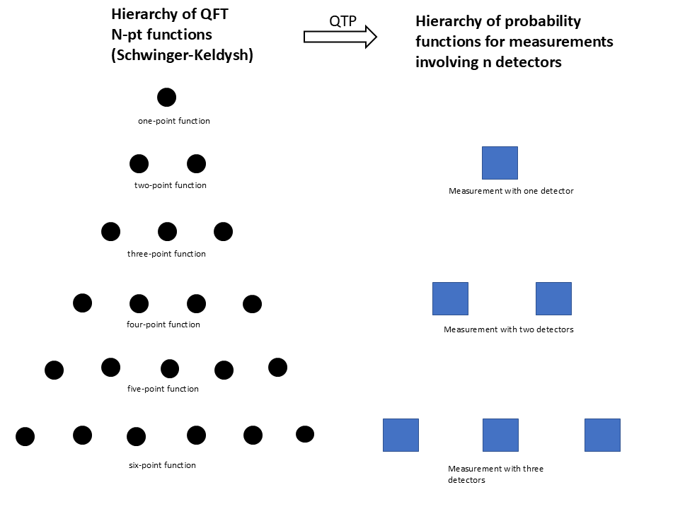
Figure 1: The hierarchy of correlation functions in relation to the hierarchy of probabilities for multi-detector measurements.

In this paper, we identify the irreducibly quantum characteristics in QTP probability hierarchies, and, consequently, of the associated CTP field correlation functions. The key observation is that classical probabilistic hierarchies are subject to constraints, due to compatibility conditions between the different levels of the hierarchy. We show that these constraints are violated in quantum theory. Then, the size of this violation, as quantified by a norm, defines a quantum resource associated to the probabilistic hierarchy.

We identify two types of classicality conditions in probabilistic hierarchies, Kolmogorov additivity and measurement independence.

1. A probabilistic hierarchy can be obtained from a single stochastic probability measure, if it satisfies Kolmogorov additivity. This is a compatibility condition between any level of the hierarchy and its lower ones. Quantum theory can violate Kolmogorov additivity, a feature that has also been identified in non-relativistic set-ups [57, 58, 59], and it is closely related to the violation of the Leggett-Garg inequalities [60, 61].

2. A hierarchy that satisfies Kolmogorov additivity is described by a stochastic process, but this process is not necessarily local. The appropriate locality condition is measurement independence [62, 63, 64], which roughly asserts that the physical quantity that is being measured in a detector is defined independently of any other quantity that is being measured in the same set-up. In non-relativistic physics, measurement independence is a prerequisite for the derivation of Bell’s inequality.

The two conditions above constrain probability densities from different levels in the probabilistic hierarchy. This contrasts Bell-type inequalities [4] that–in the present context–require the comparison of probability densities from different probabilistic hierarchies. For example, the derivation of the Clauser-Horne-Shimony-Holt (CHSH) inequality [65] considers four different pairs of detectors, and each pair would have to be embedded at the level $n=2$ of a different probabilistic hierarchy.

In this paper, we analyze the implications of the classicality constraints above, and then we define the quantum resources defined by their violation. For concreteness, we evaluate the latter for the simplest probabilistic hierarchy. This consists of probability densities of the form (1), in which the only recorded observable is the spacetime point of the detection event. Hence, the hierarchy consists of probability densities of the form $p_{n}(x_{1},x_{2},\ldots,x_{n})$ for $n$ detection events at spacetime points $x_{1},x_{2},\ldots,x_{n}$. Such probability densities enable us to undertake an analysis of Einstein causality in QFT measurements. The analysis simplifies significantly when considering a set-up of small detectors at fixed spatial locations. Them, the only random variables are the detection times $t_{1},t_{2},\ldots,t_{n}$ in each apparatus.

We find that the violation of both constraints is generic, and, in principle, measurable. Kolmogorov additivity is violated in set-ups where particles are detected sequentially by two detectors, and it is due to the change of the quantum state after the first detection. Measurement independence is violated in multi-partite systems. In the cases analyzed here, it is related to entanglement between recorded particles.

The plan of this paper is the following. In Sec. 2, we summarize the main points of the QTP method for measurements in QFT. In Sec. 3, we analyse the classicality conditions of probabilistic hierarchies and we define the corresponding quantum resources. In Sec. 4, we focus on the violation of measurement independence in a bipartite system. In Sec. 5, we analyse the violation of Kolmogorov additivity. In Sec. 6, we summarize and discuss our results.

2 Background

In this section, we present the main points of the QTP formalism, as presented in Ref. [7], and we setup the notation for the rest of this paper.

Consider a general quantum field theory defined by a Hilbert space ${\cal F}$. The quantum field interacts with $n$ detectors, each localized in different spatial region, and described by the Hilbert space ${\cal H}_{i}$, for $i=1,2,\ldots,n$. Each detector records the time and location of a particle-detection event, and also the value of additional observables (e.g., four momentum, angular momentum), collectively labeled by $q$. The state of motion of the detectors may be arbitrary.

The quantum field interacts with the $i$-th detector through an interaction term of the form

$$\hat{V}_{i}=\int d^{4}x\hat{C}^{(i)}_{a}(x)\hat{J}_{(i)}^{a}(x),$$ (3)

where $\hat{C}_{a}^{(i)}(x_{i})$ is a field composite operator that defines the channel of interaction between field and detector and here $\hat{J}_{(i)}^{a}(x)$ is a (Heisenberg-picture) current on the detector Hilbert space ${\cal H}_{i}$. The index $a$ is composite, and it may include spacetime, spinor, and internal indices. Raising and lowering the indices occurs, so that expressions of the form $K_{a}L^{a}$ are spacetime scalars.

Some examples of relevant composite operators include

• dipole coupling $\hat{C}(x)=\hat{\phi}(x)$ for a scalar field $\hat{\phi}(x)$,

• coupling for detection through scattering $\hat{C}(x)=:\hat{\phi}^{2}(x):$ for a scalar field $\hat{\phi}(x)$,

• scalar and vector couplings $\hat{C}(x)=:\hat{\bar{\psi}}(x)\hat{\psi}(x):$ and $\hat{C}^{\mu}(x)=:\hat{\bar{\psi}}(x)\gamma^{\mu}\hat{\psi}(x):$, respectively, for a Dirac field $\hat{\psi}(x)$.

The QTP analysis leads to an unnormalized probability density for the $n$ measurement events,

$$P_{n}(x_{1},q_{1};x_{2},q_{2};\ldots;x_{n},q_{n})=\int d^{4}y_{1}\ldots d^{4}y_{n}R_{(1)}^{a_{1}b_{1}}(y_{1},q_{1})\ldots R_{(n)}^{a_{n}b_{n}}(y_{n},q_{n})$$

$$\times G_{a_{1}\ldots a_{n},b_{1}\ldots b_{n}}(x_{1}-\frac{1}{2}y_{1},\ldots,x_{n}-\frac{1}{2}y_{n};x_{1}+\frac{1}{2}y_{1},\ldots,x_{n}+\frac{1}{2}y_{n}),$$ (4)

where $x_{i}$ are spacetime coordinates of a detection event. The probability density is a linear functional of the $2n$-unequal-time correlation function and

$$G_{a_{1}\ldots a_{n},b_{1}\ldots b_{n}}(x_{1},\ldots,x_{n};x_{1}^{\prime},\ldots,x_{n}^{\prime})=\langle\psi|{\cal T}^{*}[\hat{C}_{b_{1}}^{(1)}(x^{\prime}_{1})\ldots\hat{C}_{b_{n}}^{(n)}(x^{\prime}_{n})]$$

$$\times{\cal T}[\hat{C}_{a_{n}}^{(n)}(x_{n})\ldots\hat{C}_{a_{1}}^{(1)}(x_{1})]|\psi\rangle$$ (5)

of the field composite operators $\hat{C}_{a_{i}}^{(1)}(x_{i})$.

The quantities $R^{ab}_{(i)}(x,q)$ in Eq. (4) are the detector kernels of each measurement. They contain all information pertaining to the detector, including its internal dynamics and its state of motion. The expressions for the detector kernel simplify under the following two assumptions.

1. A detector follows an inertial trajectory in Minkowski spacetime.

2. A detector is initially prepared on a state $|\Omega\rangle$ that is approximately translation invariant. Heuristically, this means that the apparatus is prepared in an state that is homogeneous at the length scales relevant to position sampling and approximately static at the time scales that relevant to time sampling.

Then, the detector kernel takes the form

$$R^{ab}(x,q)=\langle a,q|e^{i\hat{p}\cdot(x-x_{0})}|b,q\rangle,$$ (6)

where $x_{0}$ is a reference point in the world-tube of the detector, and $|a,q\rangle=\sqrt{\hat{\Pi}(q)}\hat{J}(x_{0})|\Omega\rangle$. Here, $\hat{\Pi}(q)$ is a set of positive operators on the Hilbert space of a single detector, that is correlated to the values of the observable $q$. It satisfies $\sum_{q}\hat{\Pi}(q)=\hat{I}-|\Omega\rangle\langle\Omega|$. Some explicit models for detector kernels are described in the Appendix B.

The Fourier transform of the detector kernel

$$\tilde{R}^{ab}(\xi,q)=\int d^{4}xe^{-i\xi\cdot x}R^{ab}(x,q),$$ (7)

is given by

$$\tilde{R}^{ab}(\xi,q)=(2\pi)^{4}e^{i\xi\cdot x_{0}}\langle a,q|\hat{E}_{\xi}|b,q\rangle,$$ (8)

where $\hat{E}_{\xi}=\delta^{4}(\hat{p}-\xi)$ is the projector onto the subspace with four-momentum $\xi^{\mu}$. The momentum four vector associated to the detector is timelike and the associated energy $p^{0}$ is positive. This means that $\tilde{R}^{ab}(p,q)=0$ for spacelike $p$, or if $p^{0}<0$. Eq. (8) also implies that $\tilde{R}^{ab}(\xi,q)\geq 0$, since $\langle a,q|\hat{E}_{\xi}|a,q\rangle\geq 0$.

It is convenient to express the probability densities using an abstract index notation. We use small Greek indices $\alpha,\beta,\gamma\ldots$ for the pairs $(x,a)$ where $x$ is a spacetime point and $a$ the internal index for the composite operators $\hat{C}_{a}$. All indices in a time-ordered product are upper, and all indices in an anti-time-ordered product are lower. Hence, we write the correlation functions (5) as

$$G^{\alpha_{1}\alpha_{2}\ldots\alpha_{n}}{}_{\beta_{1}\beta_{2}\ldots\beta_{n}}$$

We denote by $z$ the pairs $(x,q)$, where $x$ is a spacetime point and $q$ any other recorded observable. In this shorthand, we include in $z$ also the event $\emptyset$ of no detection. If we denote by $\Gamma$ the set of possible values for $q$, then $z$ takes values on the set $Z:=M\times\Gamma\cup\{\emptyset\}$. We will write the kernel

$$\delta[x-\frac{1}{2}(y+y^{\prime})]R^{ab}(y-y^{\prime},q)$$ (9)

as $R_{\alpha}{}^{\beta}(z)$ where $\alpha$ stands for $(y,a)$, $\beta$ for $(y^{\prime},b)$ and $z$ for $(x,q)$. The matrices $R_{\alpha}{}^{\beta}(z)$ are self-adjoint by construction: $R^{\alpha}{}_{\beta}=(R_{\alpha}{}^{\beta})^{*}$.

Then, the probability formula (4) becomes

$$P_{n}(z_{1},z_{2},\ldots,z_{n})=G^{\alpha_{1}\alpha_{2}\ldots\alpha_{n}}{}_{\beta_{1}\beta_{2}\ldots\beta_{n}}\;\;{}^{(1)}R_{\alpha_{1}}{}^{\beta_{1}}(z_{1})\;{}^{(2)}R_{\alpha_{2}}{}^{\beta_{2}}(z_{2})\ldots\;{}^{(n)}R_{\alpha_{n}}{}^{\beta_{n}}(z_{n}).$$ (10)

In this notation, each measurement event is associated to a pair of indices in the correlation function, an upper one $\alpha_{i}$ and a lower one $\beta_{i}$.

In some cases, it will be useful to further condense the notation, and employ DeWitt notation, in which each pair $(\alpha_{i},\beta_{i})$ corresponds to a single capital index $A_{i}$. Hence, we will write the 2n-point correlation function as $G_{A_{1},\ldots,A_{n}}$ and the detector kernels as $R^{A}(z)$. Then, the probability formula (10) reads

$$P_{n}(z_{1},z_{2},\ldots,z_{n})=G_{A_{1}A_{2}\ldots A_{n}}R_{1}^{A_{1}}(z_{1})R_{2}^{A_{2}}(z_{2})\ldots R_{n}^{A_{n}}(z_{n})$$ (11)

Each vector $v_{A}$ corresponds to a matrix $v_{\alpha}{}^{\beta}$, and we can define the Hilbert-Schmidt inner product

$$(v,w)=Tr(vw^{\dagger}).$$ (12)

Hence, the space ${\cal V}$ of vectors $v_{A}$ with finite norm $||v||=\sqrt{v_{A}\bar{v}^{A}}$ defines a Hilbert space. The inner product allows us to raise and lower the capital indices consistently. In particular, we will denote the Riesz-dual of a vector $v_{A}$ by $\bar{v}^{A}$. We will also define the norm of any “tensor“ $G_{A_{1},\ldots,A_{n}}$ as $||G||:=\sqrt{G_{A_{1},\ldots,A_{n}}\bar{G}^{A_{1},\ldots,A_{n}}}$.

3 Measures of non-classicality

In this section, we analyze the structure of the hierarchy of QTP probability functions, and we identify behavior with no classical analogue. We also define informational quantities that quantify the degree if irreducible non-classicality.

3.1 Non-additivity in the hierarchy of probability densities

Suppose that we have a specific rule for selecting the type of apparatuses that appear in the $n$-event measurement described by the probability distribution (4), for all $n=1,2,\ldots$. The simplest such rule is to assume that all apparatuses are identical, modulo a spacetime translation of their worldtubes, so that the associated detector kernels differ only by a phase term $e^{i\xi\cdot a}$ in the Fourier space. We can absorb such phase differences in a redefinition of the observables $z_{i}$, so that $R^{A}_{i}(z)=R^{A}(z)$ for all $i$.

Given such a rule, Eq. (10) assigns to each initial state $|\psi\rangle$ of the field a hierarchy of joint probability distributions $P_{n}(z_{1},z_{2},\ldots,z_{n})$, where $n=1,2,\ldots,$. We can define a moment-generating functional for all probability densities (10), in terms of sources $j(z)$,

$$Z_{QTP}[j]=\sum_{n=0}^{\infty}\sum_{z_{1},z_{2},\ldots,z_{n}}\frac{i^{n}}{n!}P_{n}(z_{1},z_{2},\ldots,z_{n})j(z_{1})\ldots j(z_{n}),$$ (13)

where we took $p_{0}=1$.

In classical probability theory, a hierarchy of correlation functions defines a stochastic process, if it satisfies the Kolmogorov additivity condition,

$$P_{n-1}(z_{1},\ldots,z_{i-1},z_{i+1},\ldots,z_{n})=\int dz_{i}P_{n}(z_{1},\ldots,z_{i-1},z_{i},z_{i+1},\ldots,z_{n})$$ (14)

for all $i=1,2,\ldots n$ and $n=1,2,\ldots$.

Quantum probability distributions for sequential measurements do not satisfy this condition [57]. Typical probabilities for non-relativistic measurements are of the form

$$P_{2}(z_{1},z_{2})=\langle\psi|\hat{P}_{z_{1}}\hat{Q}_{z_{2}}\hat{P}_{z_{1}}|\psi\rangle,$$ (15)

for $n=2$, where $\hat{P}_{z_{1}}$ and $\hat{Q}_{z_{2}}$ are the spectral projectors associated to the first and the second measurement, respectively. If the projectors $\hat{P}_{z}$ and $\hat{Q}_{z^{\prime}}$ do not commute, then the Kolmogorov condition is typically violated. QTP probabilities have a more complicated structure, but they follow a similar pattern. The violation of the Kolmogorov condition is related the violation of the Leggett-Garg inequalities for macrorealism [5] that also refer to the behavior of quantum multi-time probabilities.

The violation of Eq. (14) is a genuine signature of quantum dynamics; it cannot be reproduced by any classical stochastic processes. In contrast, if measurements on a quantum field approximately satisfy Eq. (14), then the measurement outcomes can be simulated by a stochastic process with $n$-time probabilities given by the probability distributions (14). Then, the generating functional $Z_{QTP}$ is the functional Fourier transform of a classical stochastic probability measure.

Hence, Eq. (14) provides unambiguous classicality criterion. The divergence of a probabilistic hierarchy from Eq. (14) is a measure of the hierarchy’s “quantumness”, and it can be interpreted as a quantum resource. To quantify this resource, we define the marginals of the probability density $P_{n}$,

$$\tilde{P}_{n,i}(z_{1},z_{2},\ldots,z_{n})=\int d\zeta P_{n+1}(z_{1},\ldots,z_{i},\zeta,z_{i+1},\ldots,z_{n}).$$ (16)

We denote by $w_{n,i}$ the statistical distance between the probability distributions $\tilde{P}_{n,i}$ and $P_{n}$,

$$w_{n,i}=\delta(\tilde{P}_{n,i},P_{n})=\frac{1}{2}\int d^{n}z|\tilde{P}_{n,i}(z_{1},\ldots,z_{n})-P_{n}(z_{1},\ldots,z_{n})|.$$ (17)

The smallest value for $w_{n,i}$ is $0$, obtained when $\tilde{P}_{n,i}=P_{n}$. The largest possible value for $w_{n_{i}}$ is $1$, obtained when $\tilde{P}_{n,i}$ and $P_{n}$ have disjoint supports. We define the non-additivity of the $n$-th level of the probabilistic hierarchy as

$$w_{n}=\frac{1}{n}\sum_{i=1}^{n}w_{n,i},$$ (18)

with values in $[0,1]$.

In many cases, we are only interested in the lower levels of the hierarchy. For example, if we use the hierarchy in order to describe the non-equilibrium thermodynamics of quantum fields, Boltzmann’s equation arises at the level of $n=1$, so $w_{2}$ suffices as a measure of non-additivity. To quantify non-additivity in the whole hierarchy, it suffices to specify a finite norm for the sequence $\{w_{n}\}$. Since the sequence is bounded, it is convenient to use the supremum norm, so we define the non-additivity of the hierarchy

$$W=\sup_{n}w_{n}.$$ (19)

which is guaranteed to be finite.

The non-additivity $W$ is defined to generic probabilistic hierarchies, and not only to the ones expressed by the QTP formula. In general, it is possible to exploit the QTP formula and define non-additivity measures that are expressed in terms of QFT correlation functions. We show how this works, by focussing at the level $n=2$ of the hierarchy. The probability densities $P_{1}$ and $P_{2}$ are given by

$$P_{1}(z) = C_{1}G_{A}R^{A}(z)$$ (20)

$$P_{2}(z_{1},z_{2}) = C_{2}G_{AB}R^{A}(z_{1})R^{B}(z_{2}),$$ (21)

where $C_{1}$ and $C_{2}$ are constants that implement the normalization conditions $\int dzP_{1}(z)=\int dz_{1}dz_{2}P_{2}(z_{1},z_{2})=1$. Here, we chose $R_{1}^{A}=R_{2}^{A}$

Consider now the two marginals of $P_{2}$,

$$P_{21}(z)=\int dz_{2}P_{2}(z,z_{2})=C_{2}G_{AB}R^{A}(z)D^{B},$$ (22)

$$P_{22}(z)=\int dz_{1}P_{2}(z,z_{1})=C_{2}G_{AB}D^{A}R^{B}(z),$$ (23)

where $D^{A}=\int dzR^{A}(z)$ is a kernel that accounts for the total number of detection events on the $i$-th detector. For $R^{A}(z)$ of the form (9), $D^{A}$ corresponds to the kernel $\int dqR^{ab}(y-y^{\prime},q)$. It describes detectors that records only the spacetime coordinate of an event.

Kolmogorov additivity holds only if

$$C_{2}G_{AB}D^{B}=C_{2}G_{BA}D^{B}=C_{1}G_{A}$$ (24)

Eq. (24) is equivalent to the statement that the two vectors $G_{AB}D^{B}$ and $G_{BA}D^{B}$ coincide, and they are parallel to $G_{A}$. This means that we can quantify the violation of the Kolmogorov condition by two numbers,

• the norm of the vector $G_{[AB]}D^{B}$, and

• the angle $\theta$ between the vectors $G_{BA}D^{B}$ and $G_{A}$, defined by

  $$\cos\theta=\frac{G_{BA}D^{B}\bar{G}^{A}}{||G_{A}||\,||G_{BA}D^{B}||}.$$ (25)

In many cases, $G_{AB}D^{B}$ is indeed parallel to $G_{A}$, because tracing out the last measurement does not affect the previous outcomes (unless the probabilities are post-selected). Then, all information about non-additivity is contained into the angle $\theta$.

3.2 Violation of measurement independence

If Kolmogorov additivity is satisfied, then the hierarchy of probability functions is described by a stochastic process. This means that the probabilities for a setup involving $n$ detectors remain unchanged if we add yet another detector. In non-relativistic quantum theory, this means that the observables that are being measured always commute with each other.

Certainly, the existence of a stochastic process that simulates measurement outcomes does not guarantee classicality. Classicality requires additional conditions that enforce the separability of measurements. Of particular importance is the notion of measurement independence. Measurement independence (MI) denotes the statistical independence of any parameter that affects the selection of measurement procedures from physical variables that influence the measurement outcomes. MI enters explicitly the derivation of Bell inequalities It is significantly weaker than Bell locality (BL), namely, the assumption that the result of a measurement on one system be unaffected by operations on any distant (spacelike separated) system. MI implies BL, but the converse does not hold.

In the present context, we implement MI as follows. Suppose that the stochastic process is described by the random variables $\xi$; typically, $\xi$ are elements of a space $\Pi$ of paths over a single-time sample space. Observables are functions on $\Pi$. Suppose that we measure an observable $Z$ with values $z$; each measurement outcome is represented by a subset $C_{z}$ of $\Pi$. Let us denote by $F_{z}$, the characteristic function of $C_{z}$. By definition, $F_{z}^{2}=F_{z}$, and $Z=\int dzzF_{z}$. For a statistical ensemble of measurements described by a probability density $\rho(\xi)$, the probability density

$$P_{1}(z)=\int d\xi\rho(\xi)F_{z}(\xi)$$ (26)

describes measurements of the observable $Z$. For unsharp measurements, the condition $F_{z}^{2}=F_{z}$ can be relaxed; it suffices that $F_{z}$ be positive.

Suppose that we make $n$ independent measurements of observables $Z_{1},Z_{2},\ldots,Z_{n}$. MI implies that we can assign a different function $F^{(i)}_{z_{i}}(\xi)$ to each observable. Then, the joint probability density $P_{n}(z_{1},z_{2},\ldots,z_{n})$ takes the form

$$P_{n}(z_{1},z_{2},\ldots,z_{n})=\int d\xi\rho(\xi)F^{(1)}_{z_{1}}(\xi)F^{(2)}_{z_{2}}(\xi)\ldots F^{(n)}_{z_{n}}(\xi).$$ (27)

Probability densities of this form are severely constrained. To see this, assume that it is possible to have a set-up where $z_{2}\rightarrow z_{1}$. Then, by Jensen’s inequality,

$$P_{n}(z_{1},z_{1},\ldots,z_{n})\geq P_{n-1}(z_{1},z_{3},\ldots,z_{n})^{2}$$ (28)

For $n=2$, Eq. (28) becomes

$$P_{2}(z,z)\geq P_{1}(z)^{2}.$$ (29)

Setting $A(\xi)=\sqrt{\rho(\xi)}F^{(1)}_{z_{1}}(\xi)\ldots F^{(m)}_{z_{m}}(\xi)$, $B(\xi)=\sqrt{\rho(\xi)}F^{(m+1)}_{z_{1}}(\xi)\ldots F^{(n)}_{z_{m}}(\xi)$ for $m<n$, we write $P_{n}=\int d\xi A(\xi)B(\xi)$.Then, the Cauchy-Schwartz inequality yields

$$P_{n}(z_{1},z_{2},\ldots,z_{n})\leq\sqrt{P_{2m}(z_{1},z_{1},\ldots,z_{m},z_{m})P_{2n-2m}(z_{m+1},z_{m+1}\ldots,z_{n},z_{n})}.$$ (30)

In particular, for $n=2$,

$$P_{2}(z_{1},z_{2})\leq\sqrt{P_{2}(z_{1},z_{1})P_{2}(z_{2},z_{2})}.$$ (31)

The inequalities (30) cut across different levels of the probabilistic hierarchy in a QFT. They are loosely analogous to the violations of classicality conditions of the quantum electromagnetic field, in phenomena such as photon anti-bunching.

The simplest way to quantify quantum behavior is through the norm of the inequality violating terms. To this end, define

$$Q^{(1)}_{n}: = \int dz_{1}dz_{3}\ldots dz_{n}\max\left\{0,P_{n-1}(z_{1},z_{3},\ldots,z_{n})^{2}-P_{n}(z_{1},z_{2},\ldots,z_{n})\right\}\;\;\;$$ (32)

$$Q^{(2)}_{n,m}: = \int dz_{1}\ldots dz_{n}\max\left\{0,P_{n}(z_{1},z_{2},\ldots,z_{n})\right.$$ (33)

$$- \left.\sqrt{P_{2m}(z_{1},z_{1},\ldots,z_{m},z_{m})P_{n-m}(z_{m+1},z_{m+1}\ldots,z_{n},z_{n})}\right\}.$$

We can average $Q^{(2)}_{n,m}$ over all values of $m$ of fixed $n$, so that the number

$$Q^{(2)}_{n}=\frac{1}{m}\sum_{m=1}^{n}Q^{(2)}_{n,m}$$ (34)

quantifies the violation of measurement independence at the $n$-th level of the hierarchy. Then, the supremum norms over the sequences $\{Q^{(1)}_{n}\}$ and $\{Q^{(2)}_{n}\}$ serve as classicality measures for the whole hierarchy.

The across-levels inequalities (28, 30) are fundamentally different from Bell inequalities. The latter involve probabilities at the same level, but from different probabilistic hierarchies. For example, the CHSH inequality works at the level of $n=2$, and it connects four different probability densities $P_{2}(z_{1},z_{2})$, each corresponding to a different set-up of the measurement apparatuses. The possible scenarios for the probabilistic hierarchies in QFT are sketched in Table 1.

Probabilities in a hierarchy…	Implication
violate Kolmogorov condition	The system cannot be simulated by any stochastic process.
satisfy Kolmogorov condition, but violate measurement independence.	The system cannot be simulated by a “local” stochastic process,
satisfy Kolmogorov condition and measurement independence.	The system can be simulated by a“local” stochastic process.

Table 1: Possible behaviors of a hierarchy of probability distributions in QFT.

Consider now the specific probabilistic hierarchy defined by QTP, in which $P_{2}(z_{1},z_{2})=C_{2}G_{AB}R^{A}(z_{1})R^{B}(z_{2})$. A sufficient condition for Eq. (31) is that $G_{AB}$ is non-negative on the Hilbert space ${\cal V}$. The existence of a negative eigenvalue of $G_{AB}$ is a necessary condition for the violation of Eq. (31). Hence, the smallest negative eigenvalue of $G_{AB}$ provides a measure of the violation of Eq. (31) that depends only on the (four-point) correlation function.

4 Violation of measurement independence for scalar fields

Next, we give examples of irreducibly quantum behavior in measurements of quantum scalar fields. In this section, we will focus on the violation of measurement independence, and we will take up non-additivity in the next section.

Consider a free scalar field of mass $m$,

$$\hat{\phi}(x)=\int\frac{d^{3}k}{(2\pi)^{3/2}\sqrt{2\omega_{\bf k}}}[\hat{a}_{\bf k}e^{-ik\cdot x}+\hat{a}^{\dagger}_{\bf k}e^{ik\cdot x}],$$ (35)

expressed in terms of annihilation operators $\hat{a}_{\bf k}$ and creation operators $\hat{a}^{\dagger}_{\bf k}$; we have set $k=(\omega_{\bf k},{\bf k})$ with $\omega_{\bf k}=\sqrt{{\bf k}^{2}+m^{2}}$.

We assume scalar coupling operators $\hat{C}(x)$ to the apparatus. We will also ignore any observable other than the spacetime point of detection. For an initial field state $|\psi\rangle$, the probability density $P_{1}(x)$ for one measurement event is

$$P_{1}(x)=C_{1}\int dy\langle\psi|\hat{C}(x-\frac{1}{2}y)\hat{C}(x+\frac{1}{2}y)|\psi\rangle R(y).$$ (36)

The probability density $P_{2}(x_{1},x_{2})$ for two measurement events is

$$P_{2}(x_{1},x_{2})=C_{2}\int dy_{1}dy_{2}R_{1}(y)R_{2}(y)\langle\psi|{\cal T}^{*}[\hat{C}_{1}(x_{1}-y_{1}/2)\hat{C}_{2}(x_{2}-y_{2}/2)]$$

$${\cal T}[\hat{C}_{2}(x_{2}-y_{2}/2)\hat{C}_{1}(x_{1}+y_{1}/2)]|\psi\rangle,$$ (37)

where the two apparatuses 1 and 2 may in general be distinct: the composite operators $\hat{C}_{1,2}$ and the detection kernels $R_{1,2}$ may be different.

Note that for scalar couplings, we can always absorb the phase $e^{i\xi\cdot x_{0}}$ of Eq. (8) into a redefinition of the observables $x\rightarrow x-x_{0}$, so that $\tilde{R}$ is a positive function. Some models for the detection kernel are given in the Appendix B.

We assume an initial state that is an eigenvalue of the particle number operator. Since the composite operators are expressed in terms of creation and annihilation operators, the field state appears in the probabilities in the form of the $n$-particle reduced density matrices,

$$\rho_{n}({\bf k}_{1},{\bf k}_{2},\ldots,{\bf k}_{n};{\bf k}^{\prime}_{1},{\bf k}^{\prime}_{2},\ldots,{\bf k}^{\prime}_{n})=\langle\psi|\hat{a}^{\dagger}_{{\bf k}^{\prime}_{1}}\hat{a}^{\dagger}_{{\bf k}^{\prime}_{2}}\ldots\hat{a}^{\dagger}_{{\bf k}^{\prime}_{n}}\hat{a}_{{\bf k}_{n}}\ldots\hat{a}_{{\bf k}_{2}}\hat{a}_{{\bf k}_{1}}|\psi\rangle.$$ (38)

4.1 Probability assignment

The simplest case corresponds to identical detectors with $\hat{C}_{1}(x)=\hat{C}_{2}(x)=\hat{\phi}(x)$ and $R_{1}(x)=R_{2}(x)=R(x)$. We take $|\psi\rangle$ to be a state with a fixed number of particles. Then,

$$P_{1}(x)=P_{0}+C_{1}\int\frac{d^{3}k}{(2\pi)^{3/2}\sqrt{2\omega_{\bf k}}}\frac{d^{3}k}{(2\pi)^{3/2}\sqrt{2\omega_{\bf k}^{\prime}}}\hat{\rho}_{1}({\bf k},{\bf k}^{\prime})\tilde{R}\left(\frac{1}{2}(k+k^{\prime})\right)e^{-i(k-k^{\prime})\cdot x},$$ (39)

where $P_{0}=C_{1}\int\frac{d^{3}k}{2\omega_{\bf k}}\tilde{R}(k)$ is the constant rate of false alarms in this set-up. Note that in the derivation of Eq. (39), we used the fact that $\tilde{R}(k)=0$ if $k^{0}<0$.

The term $P_{0}$ is background noise to the detector, so we can drop it from the analysis. We define the positive operators $\hat{\Pi}_{x}$ on the Hilbert space of a single particle,

$$\langle{\bf k}|\hat{\Pi}_{x}|{\bf k}^{\prime}\rangle=\frac{1}{2(2\pi)^{3}\sqrt{\omega_{\bf k}\omega_{\bf k^{\prime}}}}\tilde{R}\left(\frac{1}{2}(k+k^{\prime})\right)e^{i(k-k^{\prime})\cdot x},$$ (40)

Then, we obtain $P_{1}(x)=C_{1}Tr(\hat{\rho}_{1}\hat{\Pi}_{x})$.

Similarly, we compute as $P_{2}(x_{1},x_{2})$ as a sum of two terms

$$P_{2}(x_{1},x_{2})=P^{a}_{2}(x_{1},x_{2})+P^{b}_{2}(x_{1},x_{2}),$$ (41)

where

$$P^{a}(x_{1},x_{2})=\frac{C_{2}}{(2\pi)^{6}}\int\frac{d^{3}k_{1}}{\sqrt{2\omega_{\bf k_{1}}}}\int\frac{d^{3}k_{1}^{\prime}}{\sqrt{2\omega_{\bf k_{1}^{\prime}}}}\int\frac{d^{3}k_{2}}{\sqrt{2\omega_{\bf k_{2}}}}\int\frac{d^{3}k_{2}^{\prime}}{\sqrt{2\omega_{\bf k_{2}^{\prime}}}}\rho_{2}({\bf k}_{1},{\bf k}_{2};{\bf k}_{1}^{\prime},{\bf k}_{2}^{\prime})$$

$$\tilde{R}\left(\frac{1}{2}(k_{1}+k_{1}^{\prime})\right)\tilde{R}\left(\frac{1}{2}(k_{2}+k_{2}^{\prime})\right)e^{-i(k_{1}-k_{1}^{\prime})\cdot x_{1}-i(k_{2}-k_{2}^{\prime})\cdot x_{2}},$$ (42)

$$P^{b}(x_{1},x_{2})=\frac{2C_{2}}{(2\pi)^{6}}\mbox{Re}\int\frac{d^{3}k_{1}}{(2\pi)^{3}\sqrt{2\omega_{\bf k_{1}}}}\int\frac{d^{3}k_{1}^{\prime}}{\sqrt{2\omega_{\bf k_{1}^{\prime}}}}\int\frac{d^{3}k_{2}}{\sqrt{2\omega_{\bf k_{2}}}}\int\frac{d^{3}k_{2}^{\prime}}{\sqrt{2\omega_{\bf k_{2}^{\prime}}}}\rho_{2}({\bf k}_{1},{\bf k}_{2};{\bf k}_{1}^{\prime},{\bf k}_{2}^{\prime})$$

$$\tilde{R}\left(\frac{1}{2}(k_{1}-k_{1}^{\prime})\right)\tilde{R}\left(\frac{1}{2}(k_{2}^{\prime}-k_{2})\right)e^{-i(k_{1}+k_{1}^{\prime})\cdot x_{1}+i(k_{2}+k_{2}^{\prime})\cdot x_{2}}$$ (43)

The key point here is that for $m\neq 0$ the term $P^{b}$ is strongly suppressed, as it involves rapid oscillations at a time-scale of order $m^{-1}$. It is also suppressed form $m=0$, and for states with negligible support on the deep infrared.

Dropping the term $P^{b}$, we obtain

$$P_{2}(x_{1},x_{2})=C_{2}Tr\left(\hat{\rho}_{2}\hat{\Pi}_{x_{1}}\otimes\hat{\Pi}_{x_{2}}\right),$$ (44)

Hence, in this setup, the Kolmogorov additivity condition (14) is satisfied—modulo the suppressed term $P_{2}^{b}(x_{1},x_{2})$. Physically, this makes sense, because, for this choice of coupling, particles are detected by absorption: no particle that has been measured in the first detector can be recorded by the second detector.

Eq. (44) also suggests that the violation of measurement independence in this set-up is related to the entanglement in the two-particle density matrix $\hat{\rho}_{2}$. In general, entanglement is not necessary. A special case of Eq. (29) is the condition in quantum optics that the second-order coherence $g^{(2)}(\tau)$ of the electromagnetic field satisfies $g^{(2)}(0)\geq 0$. This condition is violated, for example, in experiments with anti-bunching photons [67].

4.2 Time-of-arrival probabilities

To identify quantum correlations, we specialize to a set-up that describes time-of-arrival measurements. We assume that the source is localized around ${\bf x}=0$. In a set up with one measurement event, there is a single detector at ${\bf x}$. In a set-up with two measurements, one detector is located at ${\bf x}_{1}$ and the other at ${\bf x}_{2}$—see Fig. 2. We assume that the source and the detectors are motionless. This is a relativistic generalization of the setup analyzed in Ref. [29].

If the size of the detectors is much smaller than the source-detector distances $|{\bf x}_{1}|$ and ${\bf x}_{2}$, then particles effectively propagate in one dimension, along the line from the source to detector. Hence, we will express each spacetime coordinate as a pair $(t_{i},x_{i})$, where $t_{i}$ is the time in the rest-frame where the detector is static and $x_{i}$ is the distance from the source, for $i=1,2$. It is convenient to take the positions of the detection events as fixed, and treat only detection times as random variables.

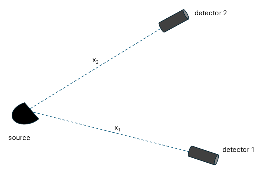
Figure 2: A two-measurement set-up: two detectors at distances $x_{1}$ and $x_{2}$ from the source. Particles effectively propagate along the line from the source to the detector.

Hence, the probability densities $P_{1}$ and $P_{2}$ become

$$P_{1}(t) = \frac{C_{1}}{2\pi}\int\frac{dk}{\sqrt{2\omega_{k}}}\frac{dk^{\prime}}{\sqrt{2\omega_{k}^{\prime}}}\rho_{1}(k,k^{\prime})\tilde{R}\left(\frac{1}{2}(k+k^{\prime}),\frac{1}{2}(\omega_{k}+\omega_{k^{\prime}})\right)$$ (45)

$$\times e^{i(k-k^{\prime})x-i(\omega_{k}-\omega_{k^{\prime}})t},$$

$$P_{2}(t_{1},t_{2}) = \frac{C_{2}}{(2\pi)^{2}}\int\frac{dk_{1}}{\sqrt{2\omega_{k_{1}}}}\frac{dk_{2}}{\sqrt{2\omega_{k_{2}}}}\frac{dk_{1}^{\prime}}{\sqrt{2\omega_{k_{1}^{\prime}}}}\frac{dk_{2}^{\prime}}{\sqrt{2\omega_{k_{2}^{\prime}}}}\rho_{2}(k_{1},k_{1}^{\prime};k_{2},k_{2}^{\prime})$$ (46)

$$\times \tilde{R}\left(\frac{1}{2}(k_{1}+k_{1}^{\prime}),\frac{1}{2}(\omega_{k_{1}}+\omega_{k_{1}^{\prime}})\right)\tilde{R}\left(\frac{1}{2}(k_{2}+k_{2}^{\prime}),\frac{1}{2}(\omega_{k_{2}}+\omega_{k_{2}^{\prime}})\right)$$

$$\times e^{i(k_{1}-k_{1}^{\prime})x_{1}+i(k_{2}-k_{2}^{\prime})x_{2}-i(\omega_{k_{1}}-\omega_{k_{1}^{\prime}})t_{1}-i(\omega_{k_{2}}-\omega_{k_{2}^{\prime}})t_{2}}.$$

Note that the quantities $k_{i}$ and $k_{i}^{\prime}$ represent here spatial momenta, and not four-momenta as in Sec. 4.1.

The detection probability for negative momentum particles is negligible for sufficiently large source-detector distances. It is therefore convenient to assume that the density matrices have support only on positive momenta, i.e., on momentum vectors in the direction from the source to the detector. In this case there a simple normalization of those probabilities when taking time to range in the full real axis,

$$\int_{-\infty}^{\infty}dtP_{1}(t)=C_{1}\int\frac{dk}{2k}\tilde{R}(k,\omega_{k})\rho_{1}(k,k).$$ (47)

The quantity $\alpha(k):=\tilde{R}(k,\omega_{k})/(2k)$ is the absorption coefficient of the detector, which gives fraction of incoming particles of momentum $k$ that are absorbed. We straightforwardly calculate

$$\int_{-\infty}^{\infty}dt_{1}\int_{-\infty}^{\infty}dt_{2}P_{2}(t_{1},t_{2})=\frac{C_{2}}{2}\int dk_{1}\alpha(k_{1})\alpha(k_{2})\rho_{2}(k_{1},k_{2};k_{1}^{\prime},k_{2}^{\prime}).$$ (48)

We can choose $C_{1}$ and $C_{2}$ so that $\int_{-\infty}^{\infty}dtP_{1}(t)=\int_{-\infty}^{\infty}dt_{1}\int_{-\infty}^{\infty}dt_{2}P_{2}(t_{1},t_{2})=1$, so that both probability densities are conditioned upon detection. We also re-define density matrices, post-selected along detection,

$$\tilde{\rho}_{1}(k,k^{\prime}) = C_{1}\rho_{1}(k,k^{\prime})\sqrt{\alpha(k)\alpha(k^{\prime})}$$ (49)

$$\tilde{\rho}_{2}(k_{1},k_{2};k_{1}^{\prime},k_{2}^{\prime}) = C_{2}\sqrt{\alpha(k_{1})\alpha(k_{2})\alpha(k_{1}^{\prime})\alpha(k_{2}^{\prime})}\rho_{2}(k_{1},k_{1}^{\prime};k_{2},k_{2}^{\prime}).$$ (50)

Then,

$$P_{1}(t)=\int\frac{dkdk^{\prime}}{2\pi}\tilde{\rho}_{1}(k,k^{\prime})\sqrt{v_{k}v_{k^{\prime}}}L(k,k^{\prime})e^{i(k-k^{\prime})x-i(\omega_{k}-\omega_{k^{\prime}})t},$$ (51)

$$P_{2}(t_{1},t_{2})=\int\frac{dk_{1}dk_{2}dk_{1}^{\prime}dk_{2}^{\prime}}{4\pi^{2}}\tilde{\rho}_{2}(k_{1},k_{2};k_{1}^{\prime},k_{2}^{\prime})\sqrt{v_{k_{1}}v_{k^{\prime}_{1}}v_{k_{2}}v_{k_{2}^{\prime}}}$$

$$\times L(k_{1},k_{1}^{\prime})L(k_{2},k_{2}^{\prime})e^{i(k_{1}-k_{1}^{\prime})x_{1}+i(k_{2}-k_{2}^{\prime})x_{2}-i(\omega_{k_{1}}-\omega_{k_{1}^{\prime}})t_{1}-i(\omega_{k_{2}}-\omega_{k_{2}^{\prime}})t_{2}},$$ (52)

where $v_{k}=k/\omega_{k}$ is the relativistic velocity, and

$$L(k,k^{\prime})=\frac{\tilde{R}\left(\frac{1}{2}(k+k^{\prime}),\frac{1}{2}(\omega_{k}+\omega_{k^{\prime}})\right)}{\sqrt{\tilde{R}(k,\omega_{k})\tilde{R}(k^{\prime},\omega_{k^{\prime}})}}$$ (53)

are the matrix elements of the localization operator $\hat{L}$. This operator is defined on the Hilbert space ${\cal H}_{1}$ of a single particle, and it determines the position spread of the detection record in the apparatus [30]. By construction, $L(k,k)=1$. Positivity of probabilities implies that $L(k,k^{\prime})\leq 1$. It can be shown that maximum localization is achieved for $L(k,k^{\prime})=1$, in which case $\hat{L}=\delta(\hat{x}_{NW})$, where $\hat{x}_{NW}$ is the Newton-Wigner position operator [68].

Maximum localization corresponds to an exponential form for the detection kernel ${\tilde{R}}(k,\omega)$,

$${\tilde{R}}(k,\omega)=\left\{\begin{array}[]{cc}A\exp\left(-\gamma_{1}|k|-\gamma_{0}\omega\right),&|k|\leq\omega,\\ 0&|k|>\omega,\;\mbox{or}\;\omega<0,\end{array}\right.$$ (56)

for some constants $\gamma_{1},\gamma_{0}\geq 0$, and $A>0$.

We can also write

$$P_{1}(t)=Tr\left(\hat{U}(x,t)\hat{\tilde{\rho}}_{1}\hat{U}^{\dagger}(x,t)\sqrt{\hat{v}}\hat{L}\sqrt{\hat{v}}\right),$$ (57)

where $\hat{U}(x,t)=e^{i\hat{p}x-i\hat{h}t}$ is a unitary operator implementing spacetime translation, $\hat{p}$ is the momentum operator, $\hat{h}=\sqrt{m^{2}+\hat{p}^{2}}$ is the Hamiltonian, and $\hat{v}=\hat{p}\hat{h}^{-1}$ is the relativistic velocity operator. This means that

$$P_{1}(t) = Tr[\hat{\tilde{\rho}}_{1}\hat{\Pi}_{x}(t)]$$ (58)

$$P_{2}(t_{1},t_{2}) = Tr[\hat{\tilde{\rho}}_{2}[\hat{\Pi}_{x_{1}}(t_{1})\otimes\hat{\Pi}_{x_{2}}(t_{2})]],$$ (59)

where the POVM $\hat{\Pi}_{x}(t)$ are defined by

$$\hat{\Pi}_{x}(t)=\sqrt{\hat{v}}\hat{U}^{\dagger}(x,t)\hat{L}\hat{U}(x,t)\sqrt{\hat{v}}.$$ (60)

For maximum localization, the POVM (60) was first derived in [69] as a relativistic generalization of Kijowski’s POVM [70] for the time of arrival.

4.3 Violation of measurement independence

An entangled state $\hat{\tilde{\rho}}_{2}$ may lead to probabilities that violate measurement independence, as expressed by Eqs. (28) and (30). To see this, we consider a pure state

$$\psi(k_{1},k_{2})=\frac{1}{\sqrt{2(1+|\epsilon|^{2})}}\left[\phi_{1}(k_{1})\phi_{2}(k_{2})+\phi_{1}(k_{2})\phi_{2}(k_{1})\right],$$ (61)

for generic single particle-states $\phi_{1}$ and $\phi_{2}$; $\epsilon=\int dk\phi_{1}(k)\phi_{2}^{*}(k)$. Assuming maximum localization, we find

$$P_{1}(t) = \frac{1}{2(1+|\epsilon|^{2})}\left[|{\cal A}_{1}(t)|^{2}+|{\cal A}_{2}(t)|^{2}+\epsilon{\cal A}_{1}(t){\cal A}_{2}^{*}(t)+\epsilon^{*}{\cal A}^{*}_{1}(t){\cal A}_{2}(t)\right],\hskip 17.07182pt$$ (62)

$$P_{2}(t_{1},t_{2}) = \frac{1}{2(1+|\epsilon|^{2})}\left|{\cal A}_{1}(t_{1}){\cal A}_{2}(t_{2})+{\cal A}_{1}(t_{2}){\cal A}_{2}(t_{1})\right|^{2},$$ (63)

where

$${\cal A}_{i}(t)=\int_{-\infty}^{\infty}dk\phi_{i}(k)\sqrt{v_{k}}e^{ikx-i\omega_{k}t}.$$ (64)

Next, we evaluate

$$w(t)=P_{1}(t)^{2}-P_{2}(t,t)=\frac{1}{4}\left[|{\cal A}_{1}(t)|^{4}+|{\cal A}_{2}(t)|^{4}-6|{\cal A}_{1}(t)|^{2}|{\cal A}_{2}(t)|^{2}\right].$$ (65)

for $\epsilon=0$. Eq. (28) is violated for

$$|{\cal A}_{1}(t)/{\cal A}_{2}(t)|\notin[\sqrt{3-2\sqrt{2}},\sqrt{3+2\sqrt{2}}]\simeq[0.41,2.41].$$ (66)

We also define

$$G(t_{1},t_{2}): = P_{2}(t_{1},t_{2})-\sqrt{P_{2}(t_{1},t_{1})P_{2}(t_{2},t_{2})}$$ (67)

$$= \frac{1}{2}\left(|{\cal A}_{1}(t_{1}){\cal A}_{2}(t_{2})|-|{\cal A}_{1}(t_{2}){\cal A}_{2}(t_{1})|\right)^{2}$$

$$- 2|{\cal A}_{1}(t_{1}){\cal A}_{2}(t_{2}){\cal A}_{1}(t_{2}){\cal A}_{2}(t_{1})|\sin^{2}\Theta(t_{1},t_{2}),$$

where $\Theta:=\frac{1}{2}(\theta_{11}+\theta_{22}-\theta_{12}-\theta_{21})$, with $\theta_{ij}:=\mbox{arg}{\cal A}_{i}(t_{j})$. Eq. (30) is violated when $G(t_{1},t_{2})>0$, or, equivalently, when

$$\sin^{2}\Theta<\frac{1}{4}\left[\frac{|{\cal A}_{1}(t_{1}){\cal A}_{2}(t_{2})|}{|{\cal A}_{1}(t_{2}){\cal A}_{2}(t_{1})|}+\frac{|{\cal A}_{1}(t_{2}){\cal A}_{2}(t_{1})|}{|{\cal A}_{1}(t_{1}){\cal A}_{2}(t_{2})|}-2\right].$$ (68)

Inequality (68) is always satisfied for $\Theta$ in a neighbourhood of $\Theta=0$. Furthermore, it is violated for all $\Theta$, if the ratio

$$\eta=\frac{|{\cal A}_{1}(t_{1}){\cal A}_{2}(t_{2})|}{|{\cal A}_{1}(t_{2}){\cal A}_{2}(t_{1})|}\notin[3-2\sqrt{2},3+2\sqrt{2}].$$ (69)

Eq. (69) is compatible with Eq. (66).

The amplitudes ${\cal A}_{i}(t)$ typically oscillate rapidly with the energy scale of the initial state. For example, if $\phi_{i}(k)$ is strongly peaked around $k=p_{i}$, we evaluate the integral (64) by expanding the phase around $k=p$. Then, we obtain

$${\cal A}_{i}(t)=v_{p_{i}}e^{i\omega_{p_{i}}t}\tilde{\phi}_{i}(x-v_{p_{i}}t),$$ (70)

where $\tilde{\phi}_{i}$ is the inverse Fourier transform of $\phi_{i}$.

For a quantitative estimate, take $p_{1}=p_{2}=p$, and use for $\phi_{1}$ and $\phi_{2}$ identical Gaussians with their centers separated by distance $a$ for $\phi_{1}$ and $\phi_{2}$ :

$$\tilde{\phi}_{1}(x)=(2\pi\sigma^{2})^{-1/4}\exp[-x^{2}/(4\sigma^{2})+ipx],\;\;\;\tilde{\phi}_{2}(x)=\phi(x-a).$$

We straightforwardly evaluate $\eta=\exp\left[\dfrac{av_{p}\Delta t}{2\sigma^{2}}\right]$, where $\Delta t=t_{2}-t_{1}$. Then, the violation of Eq. (30) is guaranteed to occur for $|\Delta t|\gtrapprox 2.5\dfrac{\sigma^{2}}{av_{p}}$. Furthermore, for $a\gtrapprox 5\sigma$, $\langle\phi_{1}|\phi_{2}\rangle<<1$, and Eq. (65) applies. It is straightforward to show that Eq. (28) is violated for $\left|t-\dfrac{L-\dfrac{1}{2}a}{v_{p}}\right|\gtrapprox 1.76\dfrac{\sigma^{2}}{av_{p}}$.

In Fig. (3), we plot the non-classicality measure $Q^{(1)}_{2}$ of Eq. (32) as a function of $a/\sigma$, for $m=0$. As expected, this increases with $a$, that is, with the size of the superposition.

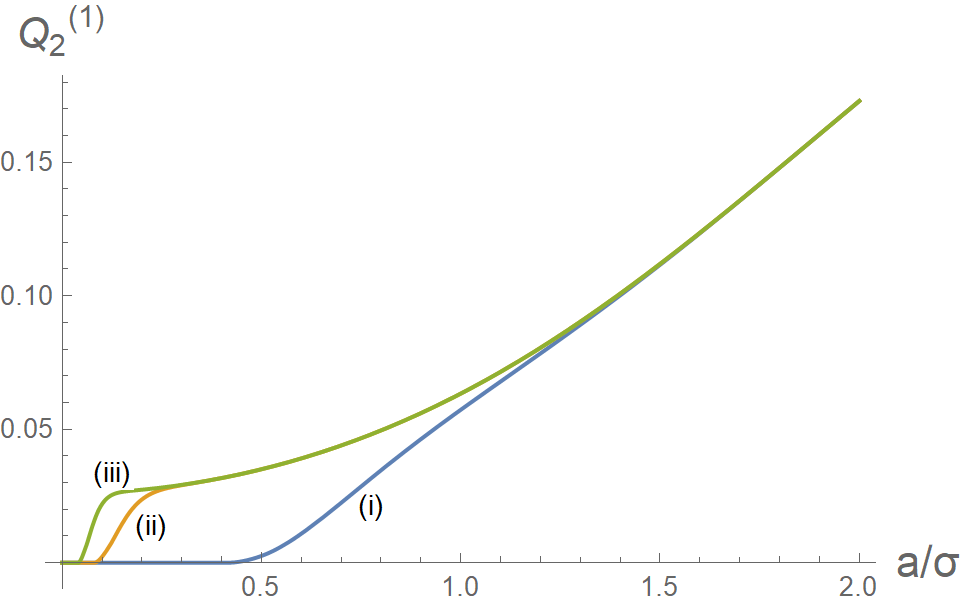
Figure 3: The measure $Q^{(1)}_{2}$ of Eq. (32) for $m=0$ as a function of $a/\sigma$ and for different values of the source-detector distance $x$: (i) $a/x=0.1$, (ii) $a/x=0.02$, and (iii) $a/x=0.01$.

Within the approximation (70), we can evaluate the non-classicality measure $Q^{(2)}_{2}=\int dt_{1}dt_{2}G(t_{1},t_{2})$ analytically. We find that

$$Q^{(2)}_{2}=1-e^{-\frac{a^{2}}{8\sigma^{2}}},$$ (71)

that is, $Q^{(2)}_{2}$ increases with the ratio $a/\sigma$, and converges rapidly to the maximum value $1$.

5 Violation of Kolmogorov additivity

In this section, we consider a model for scalar field measurements that allows us to probe the violation of Kolmogorov additivity.

5.1 The measurement model

We will again consider measurements of a single scalar field $\hat{\phi}(x)$, but now we will consider different couplings to the apparatus. For a single measurement event, we will employ the composite operator $\hat{C}_{1}(x)=:\hat{\phi}(x)^{2}:$ with detection kernel $R_{1}(x)$. For two measurement events, the first apparatus will again be described by $\hat{C}_{1}$ and $R_{1}$, but for the second apparatus we will employ $\hat{C}_{2}(x)=\hat{\phi}(x)$ with detection kernel $R_{2}$. The key point here is that the first apparatus records particles either by scattering or by double absorption. A particle that has been scattered can be absorbed by the second detector, hence, in this case a violation of Kolmogorov additivity is possible.

The calculation of the detection probabilities is straightforward if long. For a single detection event, two terms survive in the probability density $P_{1}$; for two detection events four terms survive in the probability density $P_{2}$. Their explicit expressions are given in the Appendix. The forms of these terms are expressed

Four terms survive, and their explicit expressions are given in the Appendix. Their form is represented diagrammatically in Fig. 4 for $P_{1}$ and in Fig. 5 for $P_{2}$. Each particle corresponds to two lines, one for each argument of its density matrix. Solid lines correspond to incoming particles, dashed lines correspond to particles that propagate after interaction with the first apparatus.

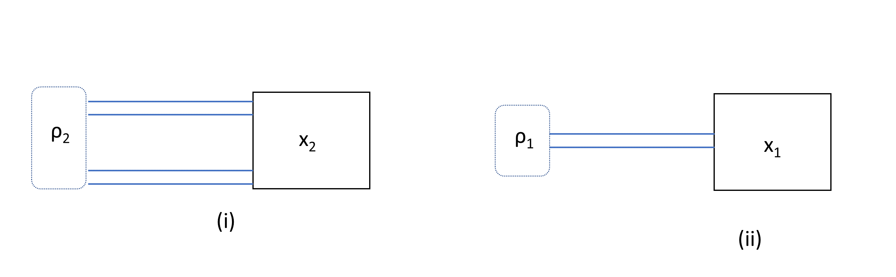
Figure 4: Diagrammatic form of the two terms that appear in the probability density $P_{1}(x)$ for a single detection event.

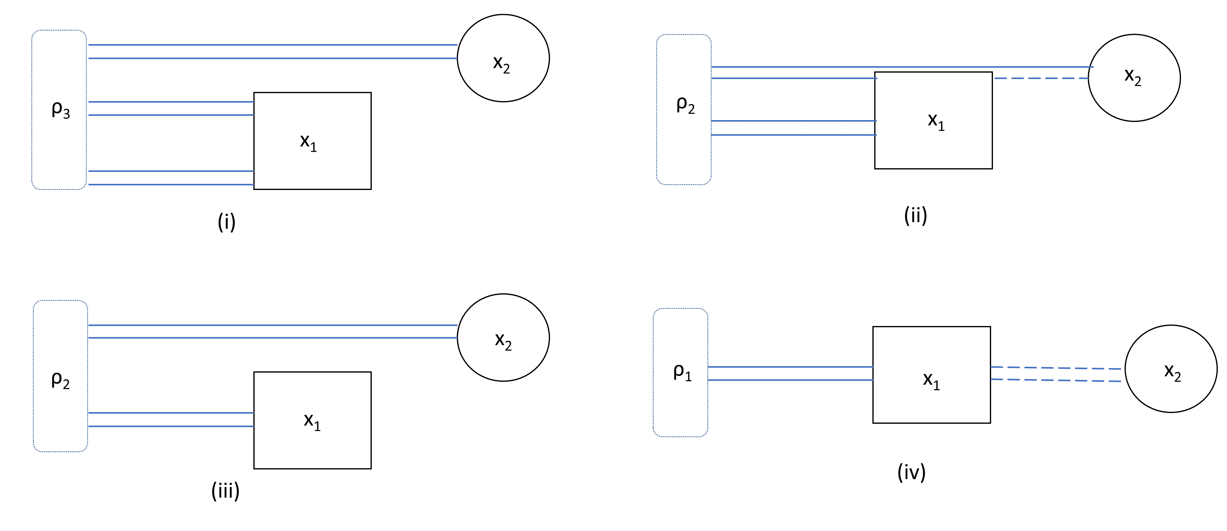
Figure 5: Diagrammatic form of the four terms that appear in the probability density $P_{2}(x_{1},x_{2})$ for two detection events.

The term (i) in $P_{1}(x)$ corresponds to simultaneous absorption of two particles, and as such it involves information from the two-particle reduced density matrix $\rho_{2}$. The term (ii) corresponds to the detection of one particle through scattering, and it involves information in the one-particle reduced density matrix.

• Terms of type (i) involve contributions to the joint detection probability from triplets of particles, two particles being detected by the first apparatus, and one particle by the second. It involves information contained in the three-particle reduced density matrix, $\rho_{3}$.

• Terms of type (ii) involve contributions from pairs of particles. One particle is detected by the first detected, and another particle is determined by the second detector, but while also receiving a contribution from particle scattering in the first detector. The information is contained in the two-particle reduced density matrix $\rho_{2}$.

• Terms of type (iii) are also determined by $\rho_{2}$. They correspond to two distinct events at the two detectors. Their contribution to the probability density is of a form similar to Eq. (42).

• Finally, terms of type (iv) are determined by the one-particle reduced density matrix $\rho_{1}(k,k^{\prime})$. They correspond to a particle being detected through scattering in the first apparatus, and then detected in the second apparatus.

Hence, the probability distribution for two detection events is a sum of four terms $P_{2}(x_{1},x_{2})=\sum_{a=1}^{4}P_{2}^{(a)}(x_{1},x_{2})$, where $P_{2}^{(a)}(x_{1},x_{2})$ corresponds to the $a$-th diagram of Fig. 5. For a single-particle state, all $n$-particle reduced density matrices vanish except for $\rho_{1}$. Hence, only diagram (ii) of Fig. 5 contributes to $P_{1}$, and only diagram (iii) of Fig. 5 contributes to $P_{2}$.

5.2 Probability assignment

We consider a set-up with two detectors, in which a particle scatters off the first detector, after leaving a measurement record, and then propagates to a second detector. The direction of scattering is a random variable; however, given a fixed position of the source and the two detectors, only particles scattered within a small solid angle along the line connecting the two detectors leave a record in both detectors. Hence, when working on the sub-ensemble of particles that leave two detection records, the scattering angle is fixed by the geometry of the configuration. Then, the only random variables are the times of detection. We denote by $t$ the detection time at detector $1$ and by $t+\tau$ the time of the second direction. We also denote the distance between the source and the first detector by $x$ and the distance between the two detectors by $r$—see Fig. 6.

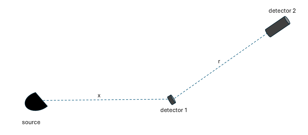
Figure 6: A set-up in which a particle is recorded by the first detector through scattering, and it is subsequently recorded by the second detector.

The probability density $P_{1}(t)$ is given by an identical expression with Eq. (45),

$$P_{1}(t)=\frac{C_{1}}{2\pi}\int\frac{dk}{\sqrt{2\omega_{k}}}\frac{dk^{\prime}}{\sqrt{2\omega_{k}^{\prime}}}\rho_{1}(k,k^{\prime})\tilde{R}_{1}^{\prime}\left(\frac{1}{2}(k+k^{\prime}),\frac{1}{2}(\omega_{k}+\omega_{k^{\prime}})\right)e^{i(k-k^{\prime})x-i(\omega_{k}-\omega_{k^{\prime}})t},$$ (72)

the only difference being that the detection kernel is given by

$$\tilde{R}_{1}^{\prime}(k,\omega)=\int\frac{dp}{\omega_{p}}\tilde{R}_{1}(k-p,\omega-\omega_{p}).$$ (73)

As in Sec. 4.2, we absorb $C_{1}$ in a redefinition $\hat{\rho}_{1}\rightarrow\hat{\tilde{\rho}}_{1}$ via Eq. (49). Then, we obtain Eq. (51) for the probability density $P_{1}(t)$ conditioned upon detection, with localization operator

$$L_{1}(k,k^{\prime})=\frac{\tilde{R}^{\prime}\left(\frac{1}{2}(k+k^{\prime}),\frac{1}{2}(\omega_{k}+\omega_{k^{\prime}})\right)}{\sqrt{\tilde{R}^{\prime}(k,\omega_{k})\tilde{R}^{\prime}(k^{\prime},\omega_{k^{\prime}})}}$$ (74)

The probability density for two detections at time $t$ and $t+\tau$, for $\tau>0$, is

$$P_{2}(t,\tau) = C_{2}\int\frac{dkdk^{\prime}}{4\pi\sqrt{\omega_{k}\omega_{k^{\prime}}}}\rho_{1}(k,k^{\prime})e^{i(k-k^{\prime})x-i(\omega_{k}-\omega_{k^{\prime}})t}\hskip 71.13188pt$$ (75)

$$\times \int\frac{dqdq^{\prime}}{4\pi\omega_{q}\omega_{q^{\prime}}}\tilde{R}_{1}\left(\frac{1}{2}(k+k^{\prime}-q-q^{\prime}),\frac{1}{2}(\omega_{k}+\omega_{k^{\prime}}-\omega_{q}-\omega_{q^{\prime}})\right)$$

$$\times \tilde{R}_{2}\left(\frac{1}{2}(q+q^{\prime}),\frac{1}{2}(\omega_{q}+\omega_{q^{\prime}})\right)e^{i(q-q^{\prime})r-i(\omega_{q}-\omega_{q^{\prime}})\tau},$$

where $C_{2}$ is a normalization constant.

The total probability of detection is

$$\int dtd\tau P_{2}(t,\tau)=C_{2}\int\frac{dk}{2k}\alpha_{2}*\tilde{R}^{\prime}_{1}(k,\omega_{k}),$$ (76)

where $\alpha_{2}*\tilde{R}^{\prime}_{1}$ is an involution of $\alpha_{2}(q)=\tilde{R}_{2}(q,\omega_{q})/(2q)$ with $\tilde{R}_{1}^{\prime}(k,\omega)$,

$$\alpha_{2}*\tilde{R}^{\prime}_{1}(k,\omega)=\int\frac{dq}{\omega_{q}}\alpha_{2}(q)\tilde{R}_{1}(k-q,\omega-\omega_{q}).$$ (77)

Hence, the total absorption coefficient for this experiment is $\alpha_{1,2}(k)=\alpha_{2}*\tilde{R}^{\prime}_{1}(k,\omega_{k})/(2k)$. We can define an initial state conditioned on detection

$$\tilde{\rho}_{1}(k,k^{\prime})=C\rho_{1}(k,k^{\prime})\sqrt{\alpha_{1,2}(k)\alpha_{1,2}(k^{\prime})},$$ (78)

so that $\int dtd\tau P_{2}(t,\tau)=1$.

We therefore obtain

$$P_{2}(t,\tau)=\int\frac{dkdk^{\prime}}{2\pi}\sqrt{v_{k}v_{k^{\prime}}}\tilde{\rho}_{1}(k,k^{\prime})e^{i(k-k^{\prime})x-i(\omega_{k}-\omega_{k^{\prime}})t}$$

$$\times\int\frac{dqdq^{\prime}}{2\pi}\sqrt{v_{q}v_{q^{\prime}}}S(k,q;k^{\prime},q^{\prime})L_{2}(q,q^{\prime})e^{i(q-q^{\prime})r-i(\omega_{q}-\omega_{q^{\prime}})\tau},$$ (79)

where $\hat{L}_{2}$ is the localization operator for the second detector, and $S(k,q;k^{\prime},q^{\prime})$ are the matrix elements of an operator $\hat{S}$ on ${\cal H}_{1}\otimes{\cal H}_{2}$

$$\langle k,q|\hat{S}|k^{\prime},q^{\prime}\rangle=\frac{\tilde{R}_{1}\left(\frac{1}{2}(k+k^{\prime}-q-q^{\prime}),\frac{1}{2}(\omega_{k}+\omega_{k^{\prime}}-\omega_{q}-\omega_{q^{\prime}})\right)}{\sqrt{\omega_{q}\omega_{q^{\prime}}\;\alpha_{2}*\tilde{R}_{1}^{\prime}(k,\omega_{k})\;\alpha_{2}*\tilde{R}_{1}^{\prime}(k^{\prime},\omega_{k^{\prime}})}}\sqrt{\alpha_{2}(q)\alpha_{2}(q^{\prime})},$$ (80)

For reasons that will be made apparent shortly, we will call $\hat{S}$ the reduction operator. This operator is self-adjoint, and invariant under the partial transposition $\langle k,q|\hat{S}|k^{\prime},q^{\prime}\rangle\rightarrow\langle k,q^{\prime}|\hat{S}|k^{\prime},q\rangle$.

The second partial trace of $\hat{S}$ is a modified version $\hat{L}_{1}^{*}$ of the localization operator $\hat{L}_{1}$, obtained by replacing $\tilde{R}_{1}^{\prime}$ by $\alpha_{2}*\tilde{R}_{1}^{\prime}$ in Eq. (74),

$$Tr_{2}\hat{S}=\hat{L}_{1}^{*}.$$ (81)

This change in the localization operator is due to the normalization of probabilities, and not an effect of the action of the second detector upon the first. In Eq. (79), we consider a statistical sub-ensemble of particles recorded at both detectors, so quantities pertaining to the first measurement have to be “averaged” with respect to the detection statistics of the second measurement. If the absorption coefficient of the second detector is constant, then $\hat{L}_{1}=\hat{L}_{1}^{*}$.

We also note that

$$\int dq\langle k,q|\hat{S}|k,q\rangle=1,$$ (82)

The operator $\hat{\sigma}_{k}$ defined by

$$\langle q|\hat{\sigma}_{k}|q^{\prime}\rangle=\langle k,q|\hat{S}|k,q^{\prime}\rangle$$ (83)

is self-adjoint. By Eq. (82), $\hat{\sigma}_{k}$ is a density matrix for an individual particle. Its diagonal elements $\langle q|\hat{\sigma}_{k}|q\rangle$ define the probability that a particle with incoming momentum $k$ is scattered towards the direction $q$. They are proportional to the differential scattering cross-section along the line that connects the two detectors.

5.3 Relativistic state reduction

The probability density $P_{2}(t,\tau)$ of Eq. (79) satisfies the Kolmogorov condition when integrating over the time $\tau$ of the second measurement,

$$\int d\tau P_{2}(t,\tau)=P_{1}(t),$$ (84)

modulo the change $\hat{L}_{1}\rightarrow\hat{L}_{1}^{*}$ for the localization operator, and the corresponding change (78) in $\hat{\rho}_{1}$, to accommodate for post-selection in the statistical ensembles. In contrast, the Kolmogorov condition is violated when integrating $P_{2}(t,\tau)$ with respect to $t$. To see this, we write

$$P(t,\tau)=\frac{1}{4\pi^{2}}Tr\left[\left(\sqrt{\hat{v}}\hat{U}^{\dagger}(r,\tau)\hat{L}_{2}\hat{U}(r,\tau)\sqrt{\hat{v}}\otimes\hat{I}\right)\right.$$

$$\left.\times\hat{S}\left(\sqrt{\hat{v}}\hat{U}(x,t)\hat{\rho}_{1}\hat{U}^{\dagger}(x,t)\sqrt{\hat{v}}\otimes\hat{I}\right)\right].$$ (85)

The conditional probability density $P(\tau|t)$ of a second detection at time $\tau$ after the first detection, given that the first detection occurred at time $t$ is given by

$$P(\tau|t)=\frac{P_{2}(t,\tau)}{P_{1}(t)}=\frac{1}{2\pi}Tr\left[\sqrt{\hat{v}}\hat{U}(r,\tau)\hat{\rho}_{1}^{(x,t)}\hat{U}^{\dagger}(r,\tau)\sqrt{\hat{v}}\hat{L}_{2}\right],$$ (86)

where

$$\hat{\rho}_{1}^{(x,t)}=\frac{1}{2\pi P_{1}(t)}\;Tr_{1}\left[\hat{S}\left(\sqrt{\hat{v}}\hat{U}(x,t)\hat{\tilde{\rho}}_{1}\hat{U}^{\dagger}(x,t)\sqrt{\hat{v}}\otimes\hat{I}\right)\right]\;$$ (87)

is the effective density matrix for the particle exiting the first detector after being recorded. It is straightforward to show that $Tr\hat{\rho}_{1}^{(x,t)}=1$. The transformation $\hat{\tilde{\rho}}_{1}\rightarrow\hat{\rho}_{1}^{(x,t)}$ is a quantum-state reduction rule for a particle recorded at the spacetime point $(x,t)$, a fact that justifies the name of the operator $\hat{S}$.

For an initial state that is almost monochromatic at momentum $k_{0}$, we can approximate $\hat{S}\simeq L_{1}^{*}\otimes\hat{\sigma}_{k_{0}}$, so that

$$\hat{\rho}_{1}^{(x,t)}\simeq\hat{\sigma}_{k_{0}},$$ (88)

that is, the effective density matrix carries no memory of the initial state, except for momentum. Otherwise, it is fully determined by the properties of the apparatus.

We emphasize that in the QTP analysis, the reduction rule follows from the form of the joint probability $P_{2}$, which ultimately derives from the decoherent histories probability assignment. Hence, the reduction rule is a derivative and not a fundamental notion. This is why the reduction rule in the first detector depends on the normalization of probabilities in the second detector. There is no action backwards in time, simply a redefinition of the relevant statistical sub-ensemble due to postselection. For other derivations of the reduction rule in analogous setups, see [29, 23, 22].

When integrating $P_{2}(t,\tau)$ with respect to $t$, we construct a probability density for $\tau$ in the second detector, with an initial state obtained from a non-selective measurement in the first detector

$$\hat{\rho}_{1}^{ns}=\int dtP_{1}(t)\hat{\rho}_{1}^{(x,t)}.$$ (89)

We straightforwardly calculate

$$\rho_{1}^{ns}(q,q^{\prime})=\int dk\tilde{\rho}_{1}(k,k)S(k,q;k,q^{\prime}),$$ (90)

or, equivalently,

$$\hat{\rho}_{1}^{ns}=\int dk\tilde{\rho}_{1}(k,k)\hat{\sigma}_{k}.$$ (91)

Hence, the state of the statistical ensemble after measurement is determined by the properties of the detector, as expressed by the density matrices $\hat{\sigma}_{k}$. All information about the off-diagonal elements of $\hat{\rho}_{1}$ in the momentum basis is lost. The diagonal elements of $\hat{\rho}_{1}$ provide the weight of the contribution of $\hat{\sigma}_{k}$ of different momenta in the final state.

The measure of the violation of Kolmogorov inequality is the statistical distance $w_{1}$ between $\tilde{P}(\tau)=\int dtP_{2}(t,\tau)$ and $P_{1}(\tau)$. This equals

$$w_{1}=\sup_{A}\left|\int d\tau\chi_{A}(\tau)[\tilde{P}(\tau)-P_{1}(\tau)]\right|=\sup_{A}\left|Tr\left[(\hat{\rho}_{1}^{ns}-\hat{\tilde{\rho}}_{1})\hat{\Pi}_{A}\right]\right|.$$ (92)

where the supremum is over all subsets $A$ of the real line, and we wrote $\hat{\Pi}_{A}=\int\hat{\Pi}_{\tau}\chi_{A}(\tau)$. The right-hand-side of Eq. (92) is smaller than $\sup_{\hat{E}}\left|Tr\left[(\hat{\rho}_{1}^{ns}-\hat{\tilde{\rho}}_{1})\hat{E}\right]\right|$, where $\hat{E}$ ranges over all positive operators with $\hat{E}\leq\hat{I}$. The latter quantity coincides with $\frac{1}{2}Tr|\hat{\rho}_{1}^{ns}-\hat{\tilde{\rho}}_{1}|$ [71], so we obtain an upper limit

$$w_{1}\leq\frac{1}{2}Tr|\hat{\rho}_{1}^{ns}-\hat{\tilde{\rho}}_{1}|.$$ (93)

6 Conclusions

The main result of this paper is the analysis of quantum resources in QFT. We showed that the QTP description of measurements enables the construction of probabilistic hierarchies that probe the information content in the QFT hierarchy of unequal-time correlation functions. In this setting, we analyzed quantum resources, in particular ones that refer to the compatibility between different levels of the probabilistic hierarchy. We identified two types of irreducibly quantum behavior. The first is associated with the failure of Kolmogorov additivity, and the second with the failure of measurement independence. Then, we considered specific examples of those resources, by focusing on measurements in which the main random variable is the detection times of relativistic particles. A by-product of this analysis was the derivation of a reduction rule for relativistic particles that are recorded—through scattering—at a spacetime point $x$.

This paper is guided by the belief that the unequal time correlation functions are the essential physical content of QFT. This implies that any relativistic approach to quantum information must focus on the properties of the hierarchy of such correlation functions, and not on the properties of the quantum state as in non-relativistic physics. The correlation functions contain information that pertain both to the initial (and occasionally final) conditions of a QFT and to dynamics, and in a relativistic setting it is impossible to separate them.

We believe that the information measures considered here must be included in any discussion of information balance in QFT. This is particularly relevant for the discussion of information loss in black-hole evaporation. In previous work, we have shown that multi-detector measurements (carried out at finite times) reveal that the Hawking radiation is not thermal or close to thermal [72, 73]. Only the probabilities associated to single-event measurements are thermal.

In this paper, we quantified quantum behavior using simple $L^{1}$ and supremum norms for the violation of classicality conditions. Entropic measures might be more appropriate for applications to non-equilibrium QFT. We recall that the level $n=1$ of the probabilistic hierarchy is the level at which the Boltzmann equation—and the thermodynamic entropy—is defined [48]. A relation between thermodynamic entropy and entropic measures of quantum correlations from the higher field correlations could be important for understanding the origins of macroscopic irreversibility.

Our longer term aim is to define quantum resources with reference solely to the hierarchy of correlation functions, and not in relation to specific measurement set-ups, as in this paper. This would provide a unified treatment of quantum resources in QFT that would bring together Kolmogorov non-additivity, violation of measurement independence (as defined here), and Bell-type non-locality. To this end, it is necessary to have a general characterization of all measurements admissible in QFT, i.e., to identify all POVMs that are compatible with relativistic causality. At the moment, this seems a formidable task.

We expect that the irreducible quantum behavior identified in this paper is experimentally accessible. For example, we noticed that the violation of the inequality (29) is already established in anti-bunching experiments for photons. In a future publication, we will analyse how the detection-time correlations of Sec. 4 can be assessed experimentally, possibly in quantum optics experiments in space that involve long baselines [74]. The violation of Kolmogorov additivity is more intricate, but it may be possible to employ variations of setups that test macrorealism through the violation of the Leggett-Garg inequality [75].

Finally, we note that in our analysis, the state-reduction rule arises as a secondary consequence of the probability rule for multi-detector measurements. It is certainly not a physical process, and this is why it may carry information from subsequent measurements, when we condition our statistical ensemble upon detection. This treatment of reduction is in accordance with ideas first expressed by Wigner [76], and made explicit in the decoherent histories program. Nonetheless, our methodology and the specific expressions for reduction derived here may be useful to the program of dynamical reduction [77], since these expressions are derived from a fully-fledged relativistic quantum theory.

Appendix A The two-event probability density of Sec. 5

The probability for one measurement event with $\hat{C}(x)=:\hat{\phi}(x)^{2}:$ consists of two terms, each corresponding to one of the two diagrams in Fig. (4),

$$P_{1}^{(i)}(t) = \int\frac{d^{3}qd^{3}q^{\prime}d^{3}kd^{3}k^{\prime}}{(2\pi)^{6}4\sqrt{\omega_{{\bf q}}\omega_{{\bf q}^{\prime}}\omega_{{\bf k}}\omega_{{\bf k}^{\prime}}}}\,\rho_{2}({\bf q},{\bf k};{\bf q}^{\prime},{\bf k}^{\prime})$$

$$\times \left[\tilde{R}_{1}\left(\frac{k+k^{\prime}+q+q^{\prime}}{2}\right)e^{-i(k+q-k^{\prime}-q^{\prime})\cdot x}+\tilde{R}_{1}\left(\frac{k+k^{\prime}-q-q^{\prime}}{2}\right)e^{-i(k+q-k^{\prime}-q^{\prime})\cdot x}\right],$$

$$P_{1}^{(ii)}(t) = 4\int\frac{d^{3}kd^{3}k^{\prime}}{(2\pi)^{3}2\sqrt{\omega_{{\bf k}}\omega_{{\bf k}^{\prime}}}}\,\rho_{1}({\bf k};{\bf k}^{\prime})\tilde{R}_{1}^{\prime}\left(\frac{k+k^{\prime}}{2}\right)e^{-i(k-k^{\prime})\cdot x}.$$ (94)

The probability density $P_{2}(x_{1},x_{2})$ for two measurement events for $\hat{C}_{1}(x)=:\hat{\phi}(x)^{2}:$ and $\hat{C}_{2}(x)=\hat{\phi}(x)$ receives four contributions, each corresponding to the four diagrams of Fig. 5,

$$P_{2}^{(i)} = \int\frac{d^{3}q_{1}d^{3}q_{2}d^{3}kd^{3}q_{1}^{\prime}d^{3}q_{2}^{\prime}d^{3}k^{\prime}}{(2\pi)^{9}8\sqrt{\omega_{{\bf q}_{1}}\omega_{{\bf q}_{2}}\omega_{{\bf q}^{\prime}_{1}}\omega_{{\bf q^{\prime}}_{2}}\omega_{{\bf k}}\omega_{{\bf k}^{\prime}}}}\,\rho_{3}({\bf q}_{1},{\bf q}_{2},{\bf k};{\bf q}_{1}^{\prime},{\bf q}_{2},{\bf k}^{\prime})$$ (95)

$$\times \tilde{R}_{1}\left(\frac{q_{1}+q_{2}+q_{1}^{\prime}+q_{2}^{\prime}}{2}\right)\tilde{R}_{2}\left(\frac{k+k^{\prime}}{2}\right)e^{-i(q_{1}+q_{2}-q_{1}^{\prime}-q_{2}^{\prime})\cdot x_{2}-i(k-k^{\prime})\cdot x_{2}},$$

$$P_{2}^{(ii)} = 4\int\frac{d^{3}qd^{3}q^{\prime}d^{3}kd^{3}k^{\prime}}{(2\pi)^{6}4\sqrt{\omega_{{\bf q}}\omega_{{\bf q}^{\prime}}\omega_{{\bf k}}\omega_{{\bf k}^{\prime}}}}\,\rho_{2}({\bf q},{\bf k};{\bf q}^{\prime},{\bf k}^{\prime})e^{-i(q-q^{\prime})\cdot x_{1}}$$

$$\times \left[F(k^{\prime}-q^{\prime}-q,k|x_{2}-x_{1})e^{ik^{\prime}\cdot x_{1}-ik\cdot x_{2}}+F(k^{\prime}-q^{\prime}-q,k^{\prime}|x_{2}-x_{1})e^{-ik^{\prime}\cdot x_{1}+ik\cdot x_{2}}\right]$$

$$P_{2}^{(iii)} = 4\int\frac{d^{3}qd^{3}q^{\prime}d^{3}kd^{3}k^{\prime}}{(2\pi)^{6}4\sqrt{\omega_{{\bf q}}\omega_{{\bf q}^{\prime}}\omega_{{\bf k}}\omega_{{\bf k}^{\prime}}}}\,\rho_{2}({\bf q},{\bf k};{\bf q}^{\prime},{\bf k}^{\prime})$$ (96)

$$\times \tilde{R}_{1}^{\prime}\left(\frac{q+q^{\prime}}{2}\right)\tilde{R}_{2}\left(\frac{k+k^{\prime}}{2}\right)e^{-i(q-q^{\prime})\cdot x_{1}-i(k-k^{\prime})\cdot x_{2}},$$

$$P_{2}^{(iv)} = 4\int\frac{d^{3}qd^{3}q^{\prime}}{(2\pi)^{3}2\sqrt{\omega_{{\bf q}}\omega_{{\bf q}^{\prime}}}}\,\rho_{1}({\bf q};{\bf q}^{\prime})G\left(\frac{1}{2}(q+q^{\prime})|x_{2}-x_{1}\right)e^{-i(q-q^{\prime})\cdot x_{1}}$$ (97)

where

$$F(q,q^{\prime}|x) = \int\frac{d^{3}p}{(2\pi)^{3}2\omega_{\bf p}}\tilde{R}_{1}\left(\frac{p+q}{2}\right)\tilde{R}_{2}\left(\frac{p+q^{\prime}}{2}\right)e^{-ip\cdot(x_{2}-x_{1})},$$ (98)

$$\tilde{R}_{1}^{\prime}(k) = \int\frac{d^{3}p}{(2\pi)^{3}\omega_{\bf p}}\tilde{R}_{1}(k-p),$$ (99)

$$G(q|x) = \int\frac{d^{3}pd^{3}p^{\prime}}{(2\pi)^{6}\omega_{\bf p}\omega_{\bf p^{\prime}}}\tilde{R}_{1}\left(\frac{p+p^{\prime}}{2}-q\right)\tilde{R}_{2}\left(\frac{p+p^{\prime}}{2}\right)e^{-i(p-p^{\prime})(x_{2}-x_{1})}.$$ (100)

Appendix B Detector models

In this section, we describe two simple detector models, which provide explicit expressions for the localization and reduction operators. For both models, we assume interaction terms of the for

$$\hat{V}=\int d^{4}x\hat{C}(x)\hat{J}(x),$$ (101)

that is, scalar composite operators $\hat{C}$ for the field and scalar “current” operators for the detector. We also assume that the only observable is the spacetime point of the detection event.

B.1 Detection through particle-like excitations

In this model, we assume that the excited states of the detector are particle-like, in the sense that they carry momentum. Then, $\hat{J}(x)$ can be identified with an effective scalar field for these excitations, and $R(x)$ is identified with the Wightman function

$$R(x)=\langle\Omega|\hat{J}(0)(\hat{I}-|\Omega\rangle\langle\Omega)\hat{J}(x)|\Omega\rangle=\langle\Omega|\hat{J}(0)\hat{J}(x)|\Omega\rangle,$$ (102)

assuming that $\langle\Omega|\hat{J}(0)|\Omega\rangle=0$.

Then, we can write $R(x)$ in the Kählen-Lehmann representation [78, 79]

$$R(x)=\int d\mu^{2}\rho(\mu^{2})\Delta_{(\mu)}(-x),$$ (103)

where $\rho(\mu^{2})$ is the field’s spectral density, and

$$\Delta_{(\mu)}(x)=\int\frac{d^{3}k}{(2\pi)^{3}}\frac{e^{i{\bf k}\cdot{\bf x}-i\sqrt{{\bf k}^{2}+\mu^{2}}t}}{2\sqrt{{\bf k}^{2}+\mu^{2}}}$$ (104)

is the Wightman function for a free scalar field of mass $\mu$.

We straightforwardly compute the Fourier transform

$$\tilde{R}({\bf k},\omega)=\rho(\omega^{2}-{\bf k}^{2}).$$ (105)

For the detection of particles with mass $m$ through absorption, the absorption coefficient is $\alpha(k)=\rho(m^{2})/(2k)$, and the localization operator is

$$L(k,k^{\prime})=\frac{\rho\left(\frac{1}{2}(m^{2}+\omega_{k}\omega_{k^{\prime}}-kk^{\prime})\right)}{\rho(m^{2})}$$ (106)

In the ultra-relativistic limit ($m\rightarrow 0$), $L(k,k^{\prime})\rightarrow 1$, i.e., we have maximum-localization measurements.

This model does not work for scattering-based measurements. It is straightforward to show that in this case, the diagonal matrix elements of the reduction operator, $\langle k,p|\hat{S}|k,p\rangle$, are proportional to $\rho(\mu^{2})$ for negative $\mu^{2}$, which is zero.

B.2 Pointlike detectors

In a point-like detector the dependence of $\tilde{R}(k,\omega)$ on $k$ is negligible. In this case, we can model the current operator as $\hat{J}(x)=\delta^{3}({\bf x})\hat{J}(t)$. Then, it is straightforward to show that

$$\tilde{R}(\omega)=\sum_{r}|\langle\Omega|\hat{J}(0)|E,r\rangle|^{2}$$ (107)

where $|E,r\rangle$ stands for the excited energy eigenstates of the detector, with $r$ the degeneracy parameter. The formulas for the localization operator and the reduction operator remain the same, with $\tilde{R}(\omega)$ in place of $\tilde{R}(k,\omega)$.

In Refs. [17, 30], it was shown that typically $R(t)$ must decay with a characteristic time scale $\tau$, so that histories with respect to the detection time decohere, and the probabilities for measurement outcomes are well defined. We can consider a Lorentzian ansatz

$$R(t)=\frac{B}{\pi}\frac{\tau}{t^{2}+\tau^{2}},$$ (108)

for some constant $B$. Then, $\tilde{R}(\omega)=Be^{-|\omega|\tau}$. This means that for detection through absorption, $L(k,k^{\prime})=1$, that is, we have maximum localization.

For detection through scattering, we find that

$$\tilde{R}^{\prime}(\omega)=\int_{0}^{\sqrt{\omega^{2}-m^{2}}}\frac{dp}{\omega_{p}}\tilde{R}(\omega-\omega_{p})=BN_{m\tau}\left(\frac{\omega}{m}\right),$$ (109)

where

$$N_{\alpha}(x)=\int_{0}^{x-1}\frac{dy}{\sqrt{(x-y)^{2}-1}}e^{-\alpha y}.$$ (110)

In the physically relevant regime, $\alpha>>1$, in which case, the integral above is dominated by values of $y$ near zero. Therefore, we can approximate $\sqrt{(x-y)^{2}-1}$ with $\sqrt{x^{2}-1}$, and set the upper limit of integration to infinity. We obtain $N_{\alpha}(x)\simeq(\alpha\sqrt{x^{2}-1})^{-1}$. Then,

$$\tilde{R}^{\prime}(\omega_{k})=\frac{B}{\tau k}.$$ (111)

This means that the associated localization operator is

$$L(k,k^{\prime})=\frac{k+k^{\prime}}{2\sqrt{kk^{\prime}}},$$ (112)

and the reduction operator is

$$\langle k,q|\hat{S}|k^{\prime},q^{\prime}\rangle=\tau\sqrt{\frac{kk^{\prime}}{\omega_{q}\omega_{q^{\prime}}}}e^{-\frac{1}{2}\tau(\omega_{k}+\omega_{k^{\prime}}-\omega_{p}-\omega_{p^{\prime}})}\theta(\omega_{k}+\omega_{k^{\prime}}-\omega_{p}+\omega_{p^{\prime}}).$$ (113)

The diagonal elements are

$$\langle k,q|\hat{S}|k,q\rangle=\frac{\tau k}{\omega_{q}}e^{-\tau(\omega_{k}-\omega_{q})}\theta(k-q).$$ (114)

We note that for $\tau\rightarrow\infty$, scattering becomes elastic.

References

• [1] P. Calabrese and J. Cardy, Entanglement Entropy and Quantum Field Theory: A Non-Technical Introduction, Int. J. Quant. Inform. 4, 429 (2006)
• [2] E. Witten, Notes on Some Entanglement Properties of Quantum Field Theory, Rev. Mod. Phys. 90, 45003 (2018).
• [3] E. Chitambar, D. Leung, L. Mancinska, M. Ozols, and A. Winter, Everything You Always Wanted to Know About LOCC (But Were Afraid to Ask), Commun. Math. Phys., 328, 303 (2014).
• [4] J. S. Bell, On the Einstein Podolsky Rosen Paradox, Physics 1, 195 (1964).
• [5] A. J. Leggett and A. Garg, Quantum Mechanics Versus Macroscopic Realism: Is the Flux There When Nobody Looks?, Phys. Rev. Lett. 54, 857 (1985).
• [6] C. Anastopoulos and N. Savvidou, Quantum Information in Relativity: The Challenge of QFT Measurements, Entropy 24, 4 (2022).
• [7] C. Anastopoulos, B. L. Hu, and K. Savvidou,Quantum Field Theory Based Quantum Information: Measurements and Correlations, Ann. Phys. 450, 169239 (2023).
• [8] A. Peres and D. Terno, Quantum Information and Relativity Theory, Rev. Mod. Phys. 76, 93 (2004).
• [9] M. Papageorgiou and D. Fraser, Eliminating the β€˜Impossible’: Recent Progress on Local Measurement Theory for Quantum Field Theory, Found. Phys. 54 (2023).
• [10] A. S. Blum, The State is not Abolished, It Withers Away: How Quantum Field Theory Became a Theory of Scattering, Studies in History and Philosophy of Modern Physics 60, 46 (2017).
• [11] R. J. Glauber, The Quantum Theory of Optical Coherence, Phys. Rev. 130, 2529 (1963).
• [12] R. J. Glauber, Coherent and Incoherent States of the Radiation Field, Phys. Rev. 131, 2766 (1963).
• [13] K. E. Hellwig and K. Kraus, Operations and measurements. II, Comm. Math. Phys. 16, 142 (1970).
• [14] W. G. Unruh, Notes on Black Hole Evaporation, Phys. Rev. D14, 870 (1976).
• [15] B. S. DeWitt, Quantum Gravity: the New Synthesis in β€œGeneral Relativity: An Einstein Centenary Survey”, eds. S. W. Hawking and W. Israel (Cambridge University Press, Cambridge, 1979).
• [16] R. Sorkin, Impossible Measurements on Quantum Fields, in β€œDirections in General Relativity”, eds. B. L. Hu and T. A. Jacobson (Cambridge University Press, Cambridge 1993).
• [17] C. Anastopoulos and N. Savvidou, Time-of-Arrival Probabilities for General Particle Detectors, Phys. Rev. A86, 012111 (2012).
• [18] C. Anastopoulos and N. Savvidou, Measurements on Relativistic Quantum Fields: I. Probability Assignment, arXiv:1509.01837.
• [19] K. Okamura and M. Ozawa, Measurement Theory in Local Quantum Physics, J. Math. Phys. 57, 015209 (2015).
• [20] C. J. Fewster and R. Verch, Quantum Fields and Local Measurements, Comm. Math. Phys. 378, 851 (2020).
• [21] H. Bostelmann, C. J. Fewster, and M. Ruep Impossible Measurements Require Impossible Apparatus, Phys. Rev. D 103, 025017 (2021).
• [22] C. J. Fewster, I. Jubb, and M. H. Ruep, Asymptotic Measurement Schemes for Every Observable of a Quantum Field Theory, Ann. Henri PoincarΓ© 24, 1137–(2023).
• [23] J. Polo-GΓ³mez, L. J. Garay, L. J. and E. MartΓ­n-MartΓ­nez, A Detector-Based Measurement Theory for Quantum Field Theory, Phys. Rev. D 105, 065003 (2022).
• [24] T. R. Perche, Localized Nonrelativistic Quantum Systems in Curved Spacetimes: A General Characterization of Particle Detector Models, Phys. Rev. D106, 025018 (2022).
• [25] T. R. Perche, J. Polo-GΓ³mez, B. de S. L. Torres, and E. MartΓ­n-MartΓ­nez, Particle Detectors from Localized Quantum Field Theories, Phys. Rev. D109, 045013 (2024).
• [26] A. Bednorz, General Quantum Measurements in Relativistic Quantum Field Theory, Phys. Rev. D108, 056020 (2023).
• [27] M. Papageorgiou, J. de RamΓ³n, and C. Anastopoulos. Particle-Field Duality in QFT Measurements, Phys. Rev. D109, 065024 (2024).
• [28] C. J. Fewster and R. Verch, Measurement in Quantum Field Theory, arXiv:2304.13356.
• [29] C. Anastopoulos and N. Savvidou, Time-of-Arrival Correlations, Phys. Rev. A95, 032105 (2017).
• [30] C. Anastopoulos and N. Savvidou, Time of Arrival and Localization of Relativistic Particles, J. Math. Phys. 60, 0323301 (2019).
• [31] C. Anastopoulos and N. Savvidou, Time-of-Arrival Probabilities and Quantum Measurements, J. Math. Phys. 47, 122106 (2006).
• [32] K. Savvidou, The Action Operator for Continuous-time Histories J. Math. Phys. 40, 5657 (1999); Continuous Time in Consistent Histories, gr-qc/9912076.
• [33] N. Savvidou, Space-time Symmetries in Histories Canonical Gravity, in β€œApproaches to Quantum Gravity”, edited by D. Oriti (Cambridge University Press, Cambridge 2009).
• [34] R. B. Griffiths, Consistent Quantum Theory (Cambridge University Press, Cambridge 2003).
• [35] R. OmnΓ©s, The Interpretation of Quantum Mechanics, (Princeton University Press, Princeton 1994).
• [36] R. OmnΓ©s, Understanding Quantum Mechanics (Princeton University Press, Princeton 1999).
• [37] M. Gell-Mann and J. B. Hartle, Quantum Mechanics in the Light of Quantum Cosmology, in β€œComplexity, Entropy, and the Physics of Information”, ed. by W. Zurek, (Addison Wesley, Reading 1990);
• [38] M. Gell-Mann and J. B. Hartle, Classical Equations for Quantum Systems, Phys. Rev. D47, 3345 (1993).
• [39] J.B. Hartle, Spacetime Quantum Mechanics and the Quantum Mechanics of Spacetime in β€œGravitation and Quantizations”, Proceedings of the 1992 Les Houches Summer School, ed. by B. Julia and J. Zinn- Justin, Les Houches Summer School Proceedings, Vol. LVII, (North Holland, Amsterdam, 1995); [gr-qc/9304006].
• [40] J. von Neumann, Mathematical Foundations of Quantum Mechanics (Princeton University Press, Princeton, 1955).
• [41] P. Busch, P. J. Lahti and P. Mittelstaedt, The Quantum Theory of Measurement, Lecture Notes in Physics Monographs, volume 2 (1996).
• [42] J. S. Schwinger, Brownian Motion of a Quantum Oscillator, J. Math. Phys. 2, 407 (1961).
• [43] L. V. Keldysh, Diagram Technique for Nonequilibrium Processes, Zh. Eksp. Teor. Fiz. 47, 1515 (1964).
• [44] G. Zhou, Z. Su, B. Hao and L. Yu, Equilibrium and Nonequilibrium Formalisms Made Unified, Phys. Rep. 118, 1 (1985).
• [45] B. S. DeWitt, Effective Action for Expectation Values, in β€œQuantum Concepts in Space and Time”, ed. R. Penrose and C. J. Isham (Claredon Press, Oxford, 1986)
• [46] E. Calzetta and B. L. Hu, Nonequilibrium Quantum Fields: Closed-Time-Path Effective Action, Wigner Function, and Boltzmann Equation , Phys. Rev. D37, 2878 (1988).
• [47] E. Calzetta and B. L. Hu, Closed-Time-Path Functional Formalism in Curved Spacetime, Phys. Rev. D35, 495 (1987).
• [48] E. A. Calzetta and B. L. Hu, Nonequilibrium Quantum Field Theory (Cambridge University Press, 2008).
• [49] J. Berges, Introduction to Nonequilibrium Quantum Field Theory, AIP Conf. Proc. 739, 3 (2004).
• [50] A. Kamenev, Field Theory of Non-Equilibrium Systems (Cambridge University Press, Cambridge, 2011).
• [51] J. Rammer, Quantum Field Theory of Non-equilibrium States (Cambridge University Press, Cambridge, 2009)
• [52] A. S. Wightman, Quantum Field Theory in Terms of its Vacuum Expectation Values, Phys. Rev. 101, 860 (1956).
• [53] R. F. Streater and A. S. Wightman, PCT, Spin and statistics, and All That (Princeton University Press, 2000).
• [54] H. Lehmann, K. Symanzik, and W. Zimmermann, Zur Formulierung Quantisierter Feldtheorien, Nuov. Cim. 1, 202 (1955).
• [55] E. Calzetta and B. L. Hu, Decoherence of Correlation Histories in β€œDirections in General Relativity, Vol II: Brill Festschrift”, eds B. L. Hu and T. A. Jacobson (Cambridge University Press, Cambridge, 1993).
• [56] E. Calzetta and B. L. Hu, Correlations, Decoherence, Disspation and Noise in Quantum Field Theory, in β€œ Heat Kernel Techniques and Quantum Gravity”, ed. S. A. Fulling (Texas A& M Press, College Station 1995).
• [57] C. Anastopoulos, Classical Versus Quantum Probability in Sequential Measurements, Found. Phys. 36, 1601 (2006).
• [58] J. Kofler and Č. Brukner, Condition for Macroscopic Realism Beyond the Leggett-Garg Inequalities, Phys. Rev. A87, 052115 (2013).
• [59] L. Clemente and J. Kofler, Necessary and Sufficient Conditions for Macroscopic Realism from Quantum Mechanics, Phys. Rev. A91, 062103 (2015).
• [60] J. J. Halliwell, Leggett-Garg Inequalities and No-Signaling in Time: A Quasiprobability Approach, Phys. Rev. A93, 022123 (2016).
• [61] J. J. Halliwell, Comparing Conditions for Macrorealism: Leggett-Garg Inequalities Versus No-Signaling in Time, Phys. Rev. A96, 012121 (2017).
• [62] J. S. Bell, A. Shimony, M. A. Horne, and J. F. Clauser, An Exchange on Local Beables, Dialectica 39, 85 (1985).
• [63] J. Barrett and N. Gisin, How Much Measurement Independence Is Needed to Demonstrate Nonlocality?, Phys. Rev. Lett. 106, 100406 (2011).
• [64] M. J. W. Hall, The Significance of Measurement Independence for Bell Inequalities and Locality, in β€œAt the Frontier of Spacetime”, ed. T. Asselmeyer-Maluga (Springer, Switzerland 2016),
• [65] M. F. Clauser, M. A. Horne, A. Shimony, and R. A. Holt, Proposed Experiment to Test Local Hidden-Variable Theories, Phys. Rev. Lett. 23, 880 (1969).
• [66] C. Anastopoulos,Quantum Theory: A Foundational Approach (Cambridge: Cambridge University Press, 2023).
• [67] M. O. Scully and M. S. Zubairy, Quantum Optics (Cambridge University Press, 2012).
• [68] T. D. Newton and E. P. Wigner Localized States for Elementary Systems, Rev. Mod. Phys. 21, 400 (1949).
• [69] J. LeΓ³n, Time-of-Arrival Formalism for the Relativistic Particle , J. Phys A: Math. Gen. 30, 4791 (1997).
• [70] J. Kijowski, On the Time Operator in Quantum Mechanics and the Heisenberg Uncertainty Relation for Energy and Time, Rep. Math. Phys. 6, 361 (1974).
• [71] M. Wilde, Quantum Information Theory (Cambridge: Cambridge University Press, 2013).
• [72] C. Anastopoulos and N. Savvidou, Multi-Time Measurements in Hawking Radiation: Information at Higher-Order Correlations, Class. Quant. Grav. 37, 025015 (2019).
• [73] C. Anastopoulos and N. Savvidou, How Black Holes Store Information in High-Order Correlations, Int. J. Mod. Phys. D29, 2043011 (2020).
• [74] M. Mohageg et al, The Deep Space Quantum Link: Prospective Fundamental Physics Experiments using Long-Baseline Quantum Optics, EPJ Quantum Technol. 9, 25 (2022).
• [75] C. Emary, N. Lambert, and Franco Nori, Leggett-Garg Inequalities, Rep. Prog. Phys. 77, 016001 (2014).
• [76] R. M F. Houtappel, H. van Dam, and E. P. Wigner, The Conceptual Basis and Use of the Geometric Invariance Principles, Rev. Mod. Phys. 37, 595 (1965).
• [77] G. C. Ghirardi and A. Bassi, Dynamical Reduction Models, Phys. Rep., 379, 257 (2003).
• [78] G. KΓ€llen, On the Definition of the Renormalization Constants in Quantum Electrodynamics, Helv. Phys. Acta 25, 417 (1952).
• [79] H. Lehmann, Über Eigenschaften von Ausbreitungsfunktionen und Renormierungskonstanten Quantisierter Felder, Nuov. Cim. 11, 342 (1954).