Linear Convergence of the Proximal Gradient Method for Composite Optimization Under the Polyak-Łojasiewicz Inequality and Its Variant

Abstract

We study the linear convergence rates of the proximal gradient method for composite functions satisfying two classes of Polyak-Łojasiewicz (PL) inequality: the PL inequality, the variant of PL inequality defined by the proximal map-based residual. Using the performance estimation problem, we either provide new explicit linear convergence rates or improve existing complexity bounds for minimizing composite functions under the two classes of PL inequality.

1 Introduction

In this paper, we consider the following composite minimization problem

$$\min_{x\in\mathbb{R}^{d}}F(x):=f(x)+h(x),$$ (1)

where $f:\mathbb{R}^{d}\to\mathbb{R}$ is a function with Lipschitz continuous gradient, and $h:\mathbb{R}^{d}\to\mathbb{R}\cup\{+\infty\}$ is a closed, proper and convex function. In addition, we assume that the optimal set $X_{*}(F):=\operatorname*{argmin}_{x\in\mathbb{R}^{d}}F(x)$ is nonempty. We denote the class of closed and proper convex functions by $\mathcal{F}_{0,\infty}$, the class of $L$-smooth convex functions by $\mathcal{F}_{0,L}$, and the class of $L$-smooth functions by $\mathcal{F}_{-L,L}$. For simplicity, we say that $F$ is a nonconvex composite function if $f\in\mathcal{F}_{-L,L}$ and a convex composite function if $f\in\mathcal{F}_{0,L}$.

The composite optimization problems arise in numerous applications, including compressed sensing [7], signal processing [5], and machine learning [12]. In recent years, the proximal gradient method (PGM) is a widely used method for composite optimization [2]. Define the proximal operator of $h$ at $x\in\mathbb{R}^{d}$ as

$$\mathrm{prox}_{h}(x):={\operatorname*{argmin}}_{y\in\mathbb{R}^{d}}\>\left\{h(y)+\frac{1}{2}\|y-x\|^{2}\right\}.$$

We summarise the PGM in Algorithm 1.

Algorithm 1 Proximal gradient method (PGM)

1:$x_{1}\in\mathbb{R}^{d}$, $\gamma\in(0,\frac{2}{L})$.

2:for $k=1,\ldots,N$ do

3:     $x_{k+1}=\mathrm{prox}_{\gamma h}\left(x_{k}-\gamma\nabla f(x_{k})\right)$

4:     $k=k+1$

5:end for

It is well-known that for composite functions with strongly convex $f$, the PGM achieves a linear convergence rate [2]. Relaxing the strong convexity condition while retaining a linear convergence rate of the PGM has been extensively studied in the literature. The PL inequality was initially introduced by Polyak [13], which is used to show linear convergence of gradient descent. Bolte et al. [3] derived a linear convergence rate of the PGM under the Kurdyka-Łojasiewicz (KL) inequality with an exponent of $\frac{1}{2}$ for convex composite functions. When the KL exponent is $\frac{1}{2}$, KL inequality is known as PL inequality for nonsmooth functions. Li and Pong [11] studied the calculus of the exponent of KL inequality and proved the linear convergence for iterates of the PGM when the PL inequality holds. Recently, Garrigos et al. [10] provided an explicit linear convergence rate of the PGM under the PL inequality. Zhang and Zhang [18] used a proximal map-based residual to define the generalized PL inequality for convex composite functions, and showed an explicit linear convergence rate of the PGM under this inequality.

Drori and Teboulle [8] first proposed the performance estimation problem (PEP) for the worst-case analysis of first-order methods, which is based on using a semidefinite programming (SDP) relaxation. Subsequently, PEP has been widely used for analyzing the worst-case convergence rates of various first-order methods, such as the gradient methods or its accelerated versions [8, 6], the PGM [16], the alternating direction method of multipliers [17], and the difference-of-convex algorithm [1]. While the original SDP relaxation in [8] is based on a discrete relaxation of the PEP,Taylor et. al. [15, 14] proposed an exact reformulation of the PEP by deriving the sufficient and necessary interpolation conditions for the function class $\mathcal{F}_{\mu,L}$ with $\mu\geq 0$ and $L\in(\mu,\infty]$. For a composite function with a strongly convex $f$, Taylor et al. [16] showed the exact worst-case linear convergence rates of the PGM in terms of objective function accuracy, distance to optimality, and residual gradient norm.

The main contribution of this paper is applying performance estimation to analyze the convergence of the PGM for composite functions under two classes of PL inequalities: the PL inequality, the variant of PL inequality defined by the proximal map-based residual, which we call RPL for simplicity. When the PL inequality holds, we provide the first explicit linear convergence rate for nonconvex composite functions, and improve the existing convergence results in [10] for convex composite functions. When the RPL inequality holds, we also provide the first explicit linear convergence rate for nonconvex composite function, and find a better bound than that given in [18] for convex composite functions. Furthermore, for the two classes of PL inequalities, we deduce the “optimal” constant step size based on the convergence rates obtained above. We compared in Table 1 the explicit worst-case convergence rates we obtained with the existing results in the literature.

Table 1: Comparison of different classes of functions and PL inequalities.

Fun. class	Con.	Convergence rate	Existing result
$f(x)\in\mathcal{F}_{0,L}$, $h(x)\in\mathcal{F}_{0,+\infty}$	PL	$\max\{\frac{1}{2\gamma\mu+1},\frac{(L\gamma-1)^{2}}{(L\gamma-1)^{2}-L\gamma^{2}\mu+2\gamma\mu}\}$	$\frac{1}{1+\gamma\mu(2-\gamma L)}$ [10]
	RPL	$\max\{\frac{1-\gamma\mu}{1+\gamma\mu},\frac{-2L\gamma^{2}\mu+L\gamma+3\gamma\mu-2}{L\gamma-\gamma\mu-2},\frac{(L\gamma-1)^{2}}{(L\gamma-1)^{2}-L\gamma^{2}\mu+2\gamma\mu}\}$	$\frac{1-\gamma\mu}{1+\gamma\mu}$($\gamma\in(0,\frac{1}{L})$) [18]
$f(x)\in\mathcal{F}_{-L,L}$, $h(x)\in\mathcal{F}_{0,+\infty}$	PL	$\max\{\frac{(L\gamma+1)^{2}}{(L\gamma+1)^{2}+L\gamma^{2}\mu+2\gamma\mu},\frac{(L\gamma-1)^{2}}{(L\gamma-1)^{2}-L\gamma^{2}\mu+2\gamma\mu}\}$	/
	RPL	$\frac{L+\mu\left(L\gamma-1\right)^{2}-\mu}{L}$	/

The rest of the paper is organized as follows. In Sect. 2, we provide preliminary definitions of PL inequalities and some interpolation conditions used in the proof. In Section 3, we present explicit linear convergence rates of the PGM and derive its “optimal” step size under the PL inequality. Subsequently, in Section 4, we extend our analysis to the RPL inequality setting and also establish new linear convergence results. We end the paper with some conclusions in Sect. 5.

Notation. The notation $\left<\cdot,\cdot\right>$ and $||\cdot||$ is the Euclidean inner product and norm, respectively. $A\succeq 0$ means that $A$ is a symmetric positive semi-definite matrix, and $\mathrm{tr}(A)$ stands for the trace of $A$. The distance function is denoted by $d(x,X):=\inf_{y\in X}\|x-y\|$ for any nonempty $X\subset\mathbb{R}^{d}$.

2 Preliminaries

We consider the convergence for the PGM under the following two settings, where the first consider nonconvex smooth function $f$, and the latter considers convex smooth $f$.

Condition 1.

The function $f(x)\in\mathcal{F}_{-L,L}$ and $h(x)\in\mathcal{F}_{0,+\infty}$.

Condition 2.

The function $f(x)\in\mathcal{F}_{0,L}$ and $h(x)\in\mathcal{F}_{0,+\infty}$.

We say that a smooth function $f$ satisfies the PL inequality if the following inequality holds for some $\mu>0$,

$$\frac{1}{2\mu}||\nabla f(x)||^{2}\geq(f(x)-f_{*}),\quad\forall x\in\mathbb{R}^{d}.$$ (2)

The PL inequality implies that each stationary point is a global minimum.

Let $\partial F(x)$ denote the Clarke subdifferential of a local Lipschitz function $F(x)$ We say the function $F$ satisfies the PL inequality if there exists $\mu>0$ such that

$$\frac{1}{2\mu}d(0,\partial F(x))^{2}\geq F(x)-F_{*},\quad\forall x\in\mathbb{R}^{d},$$ (3)

where $\partial F(x)=\nabla f(x)+\partial h(x)$ because $f$ is smooth [4, Proposition 2.3.3]. Note that the PL inequality here is a special case of the KL inequality ([3]) with exponent $\frac{1}{2}$.

For composite function $F(x)$, Zhang and Zhang [18] used proximal map-based residual to define the RPL inequality:

$$\exists\mu>0,\text{ such that }\|\mathcal{G}_{\gamma}(x)\|^{2}\geq 2\mu(F(x)-F_{*}),\quad\forall x\in\mathbb{R}^{d},$$ (4)

where the proximal map-based residual is defined by

$$\mathcal{G}_{\gamma}(x):=\frac{1}{\gamma}\Big{(}x-\mathrm{prox}_{\gamma h}\big{(}x-\gamma\nabla f(x)\big{)}\Big{)}.$$

Our analysis heavily depends on the PEP technique, which can be summarised as the following procedure: (1) The abstract PEP problem can be discretized as the finite-dimensional optimization problem, where interpolation conditions should be used if available. (2) By introducing the Gram matrix, the finite-dimensional optimization problem is relaxed as a convex SDP problem, which is solvable via various off-the-shelf solvers. (3) Optimal dual solutions are first obtained numerically, and then the analytical expressions are guessed and verified analytically. (4) Finally, the worst-case convergence rate is obtained by using nonnegative linear combinations of constraints in the discretized formulation of the PEP problem.

The following facts play a key role in our analysis. Consider a set of data triples $\{(x_{i},g_{i},f_{i})\}_{i\in I}$ and define the index set $I=\{1,\ldots,N,*\}$ for the iterations. Recall the following interpolation conditions for two classes of functions.

Fact 1.

[14, Theorem 3.10] The set $\{(x_{i};g_{i};f_{i})\}_{i\in I}$ is $\mathcal{F}_{-L,L}$-interpolable if and only if the following inequality holds $\forall i,j\in I$:

$$A_{i,j}=f_{j}-f_{i}-\frac{L}{4}\|x_{i}-x_{j}\|^{2}+\frac{1}{2}\langle g_{i}+g_{j},x_{j}-x_{i}\rangle+\frac{1}{4L}\|g_{i}-g_{j}\|^{2}\leq 0.$$ (5)

Fact 2.

[15, Corollary 1] The set $\{(x_{i};g_{i};f_{i})\}_{i\in I}$ is $\mathcal{F}_{0,L}$-interpolable if and only if the following inequality holds $\forall i,j\in I$:

$$B_{i,j}:=f_{j}-f_{i}+\langle g_{j},x_{i}-x_{j}\rangle+\frac{1}{2L}\|g_{i}-g_{j}\|^{2}\leq 0.$$ (6)

Fact 3.

[15, Theorem 1] The set $\{(x_{i};s_{i};h_{i})\}_{i\in I}$ is $\mathcal{F}_{0,\infty}$-interpolable if and only if the following set of conditions holds $\forall i,j\in I$:

$$C_{i,j}:=h_{j}-h_{i}+\langle s_{j},x_{i}-x_{j}\rangle\leq 0.$$ (7)

3 Linear Convergence under the PL Inequality

In this section, we investigate the linear convergence rate of the PGM under the PL inequality. Furthermore, we obtain the explicit linear convergence rate and the “optimal” step size and compare them with the existing results.

3.1 Nonconvex Composite Case

In this section, we consider the performance of the PGM under Condition 1 and assume the PL inequality (3) holds. In the following of this paper, we set the performance criterion as the objective function accuracy $F(x_{2})-F_{*}$. In this setting, the PEP for the PGM can be written as follows:

$$\max F(x_{2})-F_{*}$$ (8)

s.t. $$x_{2}\text{ is generated by Algorithm \ref{alg:the PGM} w.r.t.}F,x_{1},$$

$$\text{$f\in\mathcal{F}_{-L,L}$, $h\in\mathcal{F}_{0,\infty}$},$$

$$F(x)-F_{*}\leq\frac{1}{2\mu}d(0,\partial F(x))^{2},\forall x\in X,$$

$$F(x_{1})-F_{*}\leq\Delta,$$

$$F(x)\geq F_{*},\forall x\in\mathbb{R}^{d},$$

$$x_{1}\in\mathbb{R}^{d},$$

where $\Delta\geq 0$ denotes the difference between the optimal function value $F_{*}$ and the value of $F$ at the starting point. In addition, $F$ and $x_{1}$ are decision variables. This is an infinite-dimensional optimization problem with infinite number of constraints, and consequently intractable in general. In Section 2, Facts 1 and 3 provide necessary and sufficient conditions for the interpolation of $L$-smooth functions and closed, proper and convex functions. We can discretize problem (8) as a finite-dimensional optimization problem by using the following (in)equalities and interpolation conditions (5) and (7) in Facts 1 and 3.

First, following [16], the iteration $x_{k+1}=\mathrm{prox}_{\gamma h}\left(x_{k}-\gamma\nabla f(x_{k})\right)$ can be rewritten using necessary and sufficient optimality conditions on the definition of the proximal operator:

$$x_{k+1}=x_{k}-\gamma(g_{k}+s_{k+1})$$ (9)

for some $s_{k+1}\in\partial h(x_{k+1})$, and $g_{k}=\nabla f(x_{k})$. Note that $g_{*}+s_{*}=0$.

When the function $f$ satisfies the PL inequality (3), we directly discretize the PL inequality (3) and pick a subgradient $s_{i}\in\partial h(x_{i})$. Then we obtain

$$D_{i}:=f_{i}+h_{i}-f_{*}-h_{*}-\frac{1}{2\mu}\|g_{i}+s_{i}\|^{2}\leq 0.$$ (10)

We then use the PEP procedure outlined in Section 2, where problem (8) is discretized as a finite-dimensional optimization problem using the above (in)equalities. We then provide an explicit convergence rate of the PGM under the PL inequality (3).

Theorem 1.

Suppose that Condition 1 holds, $F$ satisfy the PL inequality (3) on $X=\{x:F(x)\leq F(x_{1})\}$, and $x_{2}$ is generated by Algorithm 1. Then the following holds.

1. If $\gamma\in\left(0,\frac{\sqrt{3}}{L}\right]$, then $F(x_{2})-F_{*}\leq\frac{(L\gamma+1)^{2}}{(L\gamma+1)^{2}+L\gamma^{2}\mu+2\gamma\mu}(F(x_{1})-F_{*}).$

2. If $\gamma\in\left(\frac{\sqrt{3}}{L},\frac{2}{L}\right)$, then $F(x_{2})-F_{*}\leq\frac{(L\gamma-1)^{2}}{(L\gamma-1)^{2}-L\gamma^{2}\mu+2\gamma\mu}(F(x_{1})-F_{*}).$

Proof.

1. First consider the case of $\gamma\in\left(0,\frac{\sqrt{3}}{L}\right]$. Let $\alpha_{1}=\frac{L^{2}\gamma^{2}+3L\gamma+2}{(L\gamma+1)^{2}+L\gamma^{2}\mu+2\gamma\mu},\alpha_{2}=\frac{L\gamma+1}{(L\gamma+1)^{2}+L\gamma^{2}\mu+2\gamma\mu},$ $\beta_{1}=\rho=\frac{(L\gamma+1)^{2}}{(L\gamma+1)^{2}+L\gamma^{2}\mu+2\gamma\mu}$, and $\lambda_{1}=\frac{L\gamma^{2}\mu+2\gamma\mu}{(L\gamma+1)^{2}+L\gamma^{2}\mu+2\gamma\mu}.$ It is obvious that $\alpha_{1},\alpha_{2},\beta_{1},\lambda_{1}$, and $\rho$ are nonnegative. We obtain that

$$F(x_{2}) -F_{*}-(\alpha_{1}-\alpha_{2})(F(x_{1})-F_{*})-\alpha_{1}A_{1,2}-\alpha_{2}A_{2,1}-\beta_{1}C_{1,2}-\lambda_{1}D_{2}$$

$$=\frac{L^{2}\gamma^{2}-3}{4L\left(L\gamma^{2}\mu+2\gamma\mu+\left(L\gamma+1\right)^{2}\right)}\|Lg_{1}\gamma+L\gamma s_{2}+g_{1}-g_{2}\|^{2}\leq 0,$$

where $A_{i,j}$ is defined in (5), $C_{1,2}$ is defined in (7), $D_{2}$ is defined in (10), and the last inequality holds since $\gamma\in(0,\frac{\sqrt{3}}{L}]$. Because the terms after the nonnegative parameters $\alpha_{1},\alpha_{2},\beta_{1},\lambda_{1}$ are nonpositive, we have $F(x_{2})-F_{*}\leq(\alpha_{1}-\alpha_{2})(F(x_{1})-F_{*}).$ We then obtain the desired result by substituting the values of $\alpha_{1}$ and $\alpha_{2}$.

2. For the case of $\gamma\in\left(\frac{\sqrt{3}}{L},\frac{2}{L}\right)$, let $\alpha_{1}=\frac{L\gamma-1}{(L\gamma-1)^{2}-L\gamma^{2}\mu+2\gamma\mu},\alpha_{2}=\frac{-L^{2}\gamma^{2}+3L\gamma-2}{(L\gamma-1)^{2}-L\gamma^{2}\mu+2\gamma\mu},$ $\beta_{1}=\rho=\frac{(L\gamma-1)^{2}}{(L\gamma-1)^{2}-L\gamma^{2}\mu+2\gamma\mu},\lambda_{1}=\frac{-L\gamma^{2}\mu+2\gamma\mu}{(L\gamma-1)^{2}-L\gamma^{2}\mu+2\gamma\mu}.$ It is obvious that $\alpha_{1},\alpha_{2},\beta_{1},\lambda_{1}$, and $\rho$ are nonnegative. By multiplying the inequalities by their respective factors and then summing them, we obtain that

$$F(x_{2}) -F_{*}-(\alpha_{1}-\alpha_{2})(F(x_{1})-F_{*})-\alpha_{1}A_{1,2}-\alpha_{2}A_{2,1}-\beta_{1}C_{1,2}-\lambda_{1}D_{2}$$

$$=\frac{-L^{2}\gamma^{2}+3}{4L\left(-L\gamma^{2}\mu+2\gamma\mu+\left(L\gamma-1\right)^{2}\right)}\|L\gamma g_{1}+L\gamma s_{2}-g_{1}+g_{2}\|^{2}\leq 0,$$

where $A_{i,j}$ is defined in (5), $C_{1,2}$ is defined in (7), $D_{2}$ is defined in (10), and the last inequality holds since $\gamma\in(\frac{\sqrt{3}}{L},\frac{2}{L})$. The remainder of the proof follows a similar approach to the first case. ∎

We remark that the parameters $\alpha_{1},\alpha_{2},\beta_{1},\lambda_{1}$, and $\rho$ are obtained from the SDP relaxation of the PEP problem, which is derived based on investigating the dual optimal solutions from numerous numerical experiments. Note that the explicit dual feasible solution and convergence rate in Theorem 1 match those of the SDP relaxation from numerical experiments.

Remark 1.

Existing literature has studied the linear convergence properties of gradient methods for nonconvex and nonsmooth functions under the PL inequality (3), e.g, Li and Pong [11] showed that if $F(x)$ satisfies the PL inequality (3), the iterative sequence $\{x_{k}\}$ converges locally linearly to a stationary point of $F(x)$. However, to the best of our knowledge, there is no explicit rate of linear convergence in existing literature. In Theorem 1, we provide the first explicit linear convergence rate of the PGM on objective function values for convex composition minimization.

The following proposition provides the “optimal” step size in the sense of minimizing the worst-case convergence rate in Theorem 1.

Proposition 2.

Suppose that $F$ satisfies the same conditions in Theorem 1. Then the “optimal” step size for the PGM with the worst-case convergence rate in Theorem 1 is given by $\frac{\sqrt{3}}{L}$ in $\gamma\in(0,\frac{2}{L})$.

Proof.

Let $\tau(\gamma)=\begin{cases}\frac{(L\gamma+1)^{2}}{(L\gamma+1)^{2}+L\gamma^{2}\mu+2\gamma\mu}&\gamma\in\left(0,\frac{\sqrt{3}}{L}\right]\\ \frac{(L\gamma-1)^{2}}{(L\gamma-1)^{2}-L\gamma^{2}\mu+2\gamma\mu}&\gamma\in\left(\frac{\sqrt{3}}{L},\frac{2}{L}\right).\end{cases}$ Note that $\tau^{\prime}(\gamma)<0$ with $\gamma\in\left(0,\frac{\sqrt{3}}{L}\right)$, and that $\tau^{\prime}(\gamma)>0$ with $\gamma\in\left(\frac{\sqrt{3}}{L},\frac{2}{L}\right)$. Note also that $\tau(\gamma)$ is continuous at $\frac{\sqrt{3}}{L}$. Hence, $\tau(\gamma)$ is decreasing at $\left(0,\frac{\sqrt{3}}{L}\right]$ and increasing at $\left(\frac{\sqrt{3}}{L},\frac{2}{L}\right)$. Therefore, the minimum value of $\tau(\gamma)$ occurs at $\frac{\sqrt{3}}{L}$. ∎

3.2 Convex Composite Case

In this section, we consider the performance of the PGM under Condition 2 and assume the PL inequality (3) holds. We still need the iteration format (9), the interpolation condition for closed, proper and convex functions (7), and the PL inequality (10) mentioned in Section 3.1. However, we replace (5) with the interpolation condition for $L$-smooth convex functions (6).

Following the PEP procedure in Section 2, we provide an explicit linear convergence rate for the PGM under the PL inequality (3).

Theorem 3.

Suppose that Condition 2 holds, $F$ satisfy the PL inequality (3) on $X=\{x:F(x)\leq F(x_{1})\}$, and $x_{2}$ is generated by Algorithm 1. Then the following holds.

1. If $\gamma\in(0,\frac{3}{2L}]$, then $F(x_{2})-F_{*}\leq\frac{1}{2\gamma\mu+1}(F(x_{1})-F_{*}).$

2. If $\gamma\in(\frac{3}{2L},\frac{2}{L})$, then $F(x_{2})-F_{*}\leq\frac{(L\gamma-1)^{2}}{(L\gamma-1)^{2}-L\gamma^{2}\mu+2\gamma\mu}(F(x_{1})-F_{*}).$

Proof.

1. First consider the case of $\gamma\in(0,\frac{3}{2L}]$. Let $\alpha_{1}=\frac{2}{2\gamma\mu+1},\alpha_{2}=\beta_{1}=\frac{1}{2\gamma\mu+1},\lambda_{1}=\frac{2\gamma\mu}{2\gamma\mu+1}.$ It is obvious that $\alpha_{1},\alpha_{2},\beta_{1}$, and $\lambda_{1}$ are nonnegative. We obtain that

$$F(x_{2}) -F_{*}-\beta_{1}(F(x_{1})-F_{*})-\alpha_{1}B_{1,2}-\alpha_{2}B_{2,1}-\beta_{1}C_{1,2}-\lambda_{1}D_{2}$$

$$=\frac{2L\gamma-3}{2(2\gamma\mu+1)}\|g_{1}-g_{2}\|^{2}\leq 0,$$

where $B_{i,j}$ is defined in (6), $C_{1,2}$ is defined in (7), $D_{2}$ is defined in (10), and the last inequality holds since $\gamma\in(0,\frac{3}{2L}]$. Because the terms after the nonnegative parameters $\alpha_{1},\alpha_{2},\beta_{1}$, and $\lambda_{1}$ are nonpositive, we have

$$F(x_{2})-F_{*}\leq\beta_{1}(F(x_{1})-F_{*})=\frac{1}{2\gamma\mu+1}(F(x_{1})-F_{*}).$$

2. For the case of $\gamma\in(\frac{3}{2L},\frac{2}{L})$, let $\alpha_{1}=\frac{L\gamma-1}{(L\gamma-1)^{2}-L\gamma^{2}\mu+2\gamma\mu},\alpha_{2}=\frac{-L^{2}\gamma^{2}+3L\gamma-2}{(L\gamma-1)^{2}-L\gamma^{2}\mu+2\gamma\mu},$ $\beta_{1}=\frac{(L\gamma-1)^{2}}{(L\gamma-1)^{2}-L\gamma^{2}\mu+2\gamma\mu},\lambda_{1}=\frac{-L\gamma^{2}\mu+2\gamma\mu}{(L\gamma-1)^{2}-L\gamma^{2}\mu+2\gamma\mu}.$ Similar to the previous case, we obtain that

$$F(x_{2}) -F_{*}-\beta_{1}(F(x_{1})-F_{*})-\alpha_{1}B_{1,2}-\alpha_{2}B_{2,1}-\beta_{1}C_{1,2}-\lambda_{1}D_{2}$$

$$=\frac{-2L\gamma+3}{2L\left(-L\gamma^{2}\mu+2\gamma\mu+\left(L\gamma-1\right)^{2}\right)}\|Lg_{1}\gamma+L\gamma s_{2}-g_{1}+g_{2}\|^{2}\leq 0,$$

where $B_{i,j}$ is defined in (6), $C_{1,2}$ is defined in (7), $D_{2}$ is defined in (10), and the last inequality holds since $\gamma\in(\frac{3}{2L},\frac{2}{L})$. The remainder of the proof follows a similar approach to the previous case. ∎

By minimizing the convergence rate in Theorem 3, the next proposition gives the “optimal” step size for the bound. The proof is similar to that of Proposition 2 and thus omitted.

Proposition 4.

Suppose that $F$ satisfies the same conditions in Theorem 3. Then the “optimal” step size for the PGM with the worst-case convergence rate in Theorem 3 is given by $\frac{3}{2L}$ in $\gamma\in(0,\frac{2}{L})$.

Comparison. Now let us compare the our convergence results with existing literature. Recently, Garrigos et al. [10] show that the convergence of the PGM (in our notation) is

$$F(x_{2})-F^{*}\leq\frac{1}{1+\gamma\mu(2-\gamma L)}(F(x_{1})-F^{*}).$$ (11)

Next we show that our rate in Theorem 3 is better than (11) by considering two intervals. When $\gamma\in(0,\frac{3}{2L}]$, due to $2-\gamma L\in[\frac{1}{2},2)$, we have

$$\frac{1}{1+2\gamma\mu}\leq\frac{1}{1+\gamma\mu(2-\gamma L)}$$

and thus our bound in Theorem 3 is tighter. Next let $\gamma\in(\frac{3}{2L},\frac{2}{L})$. Since $(L\gamma-1)^{2}\in(\frac{1}{4},1)$, we have

$$\gamma\mu(2-\gamma L)=2\gamma\mu-L\gamma^{2}\mu\leq\frac{2\gamma\mu-L\gamma^{2}\mu}{(L\gamma-1)^{2}},$$

which further implies

$$\frac{(L\gamma-1)^{2}}{(L\gamma-1)^{2}-L\gamma^{2}\mu+2\gamma\mu}=\frac{1}{1+\frac{2\gamma\mu-L\gamma^{2}\mu}{(L\gamma-1)^{2}}}\leq\frac{1}{1+\gamma\mu(2-\gamma L)}.$$

Therefore, we provide a tighter convergence rate for $\gamma\in(0,\frac{2}{L})$ than (11). In addition, the step size $\frac{1}{L}$ corresponds to the “optimal” step size for (11). When the step size is $\frac{1}{L}$, the contraction rate of (11) is $\frac{L}{L+\mu}.$ Proposition 4 shows that $\frac{3}{2L}$ give a rate $\frac{L}{L+3\mu}$, which is strictly better than (11). An illustration of the convergence rate computed by PEP with the bound (11) is shown in Figure 2.

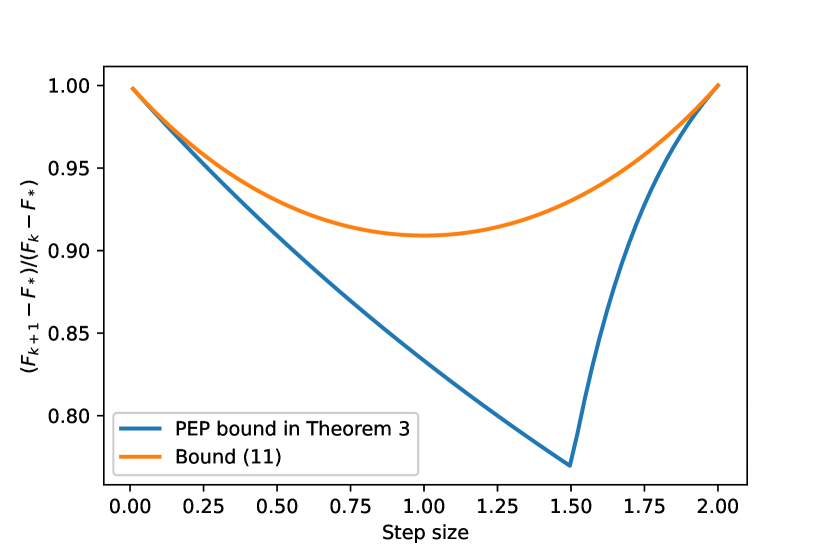
Figure 1: Comparison between convergence rates computed by PEP and bound given by (11) in [10] ($L=1$, $\mu=0.1$).

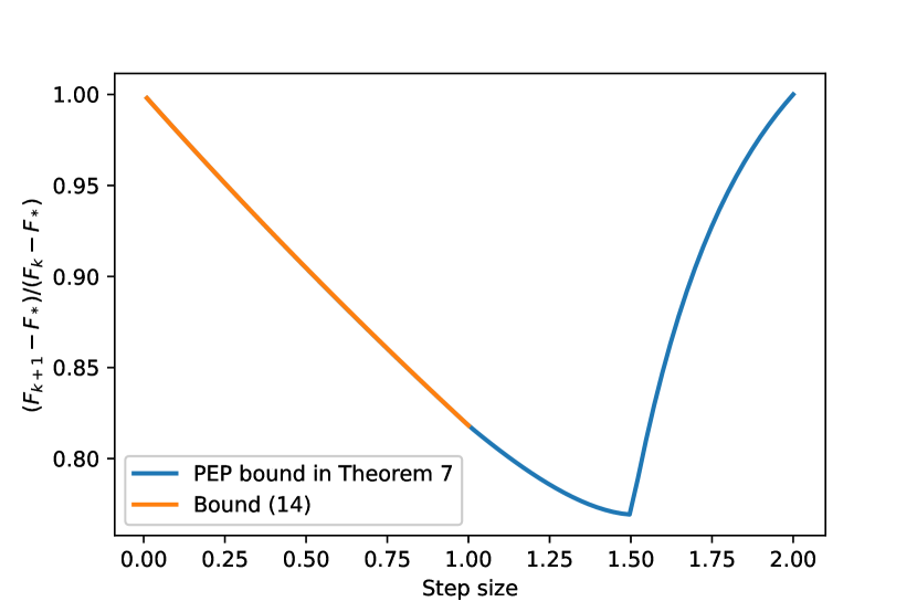
Figure 2: Comparison between convergence rates computed by PEP and bound given by (15) in [18] ($L=1$, $\mu=0.1$).

4 Linear Convergence under the RPL Inequality

In this section, we study the linear convergence of the PGM under the RPL inequality (4). We use the performance estimation to obtain the explicit linear convergence rate and the “optimal” step size.

4.1 Nonconvex Composite Case

First, we consider the performance of the PGM under Condition 1 and assume the RPL inequality (4) holds. In addition to the iteration format (9), the interpolation condition for closed, proper and convex functions (7), and the interpolation condition for $L$-smooth functions (6) mentioned in Section 2, we also need to find a discretization of (4) in a Gram-representable form. If $f$ satisfies the RPL inequality (3), we can discretize it as

$$E_{i}:=(f_{i}+h_{i})-(f_{*}+h_{*})-\frac{1}{2\mu}\|\mathcal{G}_{i}\|^{2}\leq 0,i\in\{k,k+1\},$$ (12)

where $\mathcal{G}_{i}=\mathcal{G}_{\gamma}(x_{i})$. Furthermore, plug $x_{k+1}=\mathrm{prox}_{\gamma h}(x_{k}-\gamma\nabla f(x_{k}))$ and iteration $x_{k+1}=x_{k}-\gamma(g_{k}+s_{k+1})$ into the proximal map-based residual $\mathcal{G}_{\gamma}(x_{k}):=\frac{1}{\gamma}\left(x_{k}-\mathrm{prox}_{\gamma h}(x_{k}-\gamma\nabla f(x_{k}))\right)$, we have

$$\mathcal{G}_{\gamma}(x_{k})=\frac{1}{\gamma}(x_{k}-x_{k+1})=g_{k}+s_{k+1}.$$ (13)

Therefore, the RPL inequality (4) implies

$$E^{\prime}_{k}:=(f_{k}+h_{k})-(f_{*}+h_{*})-\frac{1}{2\mu}(g_{k}+s_{k+1})^{2}\leq 0.$$ (14)

Following the PEP procedure in Section 2, we provide an explicit linear convergence rate for the PGM under the RPL inequality (4).

Theorem 5.

Suppose that Condition 1 holds, $F$ satisfy the RPL inequality (4) on $X=\{x:F(x)\leq F(x_{1})\}$, and $x_{2}$ is generated by Algorithm 1. If $\gamma\in\left(0,\frac{2}{L}\right)$, then we have

$$F(x_{2})-F_{*}\leq\frac{L+\mu\left(L\gamma-1\right)^{2}-\mu}{L}(F(x_{1})-F_{*}).$$

Proof.

Let $\alpha_{1}=\beta_{1}=1,\lambda_{1}=\frac{\mu-\mu\left(L\gamma-1\right)^{2}}{L}$ and $\rho=\frac{L+\mu\left(L\gamma-1\right)^{2}-\mu}{L}$. By multiplying the inequalities by their respective factors and then summing them, we obtain that

$$F(x_{2}) -F_{*}-\rho(F(x_{1})-F_{*})-\alpha_{1}A_{1,2}-\beta_{1}C_{1,2}-\lambda_{1}E^{\prime}_{1}$$

$$=-\frac{1}{4L}\|Lg_{1}\gamma+L\gamma s_{2}-g_{1}+g_{2}\|^{2}\leq 0.$$

where $A_{1,2}$ is defined in (5), $C_{1,2}$ is defined in (7). Because the terms after the nonnegative parameters $\alpha_{1},\beta_{1},\lambda_{1}$ are nonpositive, we have the desired result. ∎

The following proposition provides the “optimal” step size by minimizing the worst-case convergence rate in Theorem 5, whose proof is similar to that of Proposition 2 and thus omitted.

Proposition 6.

Suppose that $F$ satisfies the same conditions in Theorem 5. Then the optimal step size for the PGM with the worst-case convergence rate in Theorem 5 is given by $\frac{1}{L}$ in $\gamma\in(0,\frac{2}{L})$.

Under the RPL inequality (4), we provide the first explicit linear convergence rate of the PGM. Additionally, we show that the “optimal” step size is $\frac{1}{L}$ in this setting.

4.2 Convex Composite Case

In this section, we consider the performance of the PGM under Condition 2 and assume the RPL inequality (4) holds. Zhang and Zhang [18] proved a linear convergence rate for the PGM under the RPL inequality. By using PEP, we extend the step size interval to $(0,\frac{2}{L})$ and find a better convergence rate than that in [18]. We use the interpolation conditions of $\mathcal{F}_{0,\infty}$ in (7) and $\mathcal{F}_{0,L}$ in (6), respectively, and the discrete RPL inequality (12).

The following lemma provides the relationship between the proximal map-based residual and the distance of the subdifferential to 0, which is helpful in our analysis.

Lemma 1 (Theorem 3.5, [9]).

Let $F(x)=f(x)+h(x)$, where $f(x)\in\mathcal{F}_{0,L}$ and $h(x)\in\mathcal{F}_{0,\infty}$. For any $x\in\mathbb{R}^{d}$, it hold that $\|\mathcal{G}_{\gamma}(x)\|\leq d(0,\partial F(x)).$

Now we are ready to present our result.

Theorem 7.

Suppose that Condition 2 holds, $F$ satisfy the RPL inequality (4) on $X=\{x:F(x)\leq F(x_{1})\}$, and $x_{2}$ is generated by Algorithm 1. Then the following holds.

1. If $\gamma\in(0,\frac{1}{L}]$, then $F(x_{2})-F_{*}\leq\frac{1-\gamma\mu}{1+\gamma\mu}(F(x_{1})-F_{*}).$

2. If $\gamma\in(\frac{1}{L},\frac{3}{2L}]$, then $F(x_{2})-F_{*}\leq\frac{-2L\gamma^{2}\mu+L\gamma+3\gamma\mu-2}{L\gamma-\gamma\mu-2}(F(x_{1})-F_{*}).$

3. If $\gamma\in(\frac{3}{2L},\frac{2}{L})$, then $F(x_{2})-F_{*}\leq\frac{(L\gamma-1)^{2}}{(L\gamma-1)^{2}-L\gamma^{2}\mu+2\gamma\mu}(F(x_{1})-F_{*}).$

Proof.

1. First consider the case of $\gamma\in(0,\frac{1}{L}]$. Let $\alpha_{1}=\beta_{1}=\frac{1}{1+\gamma\mu},\lambda_{1}=\lambda_{2}=\frac{\gamma\mu}{1+\gamma\mu}.$ It is obvious that $\alpha_{1},\beta_{1},\lambda_{1}$, and $\lambda_{2}$ are nonnegative. Note that

$$\|g_{k+1}+s_{k+1}\|\geq d(0,\partial F(x_{k+1}))\geq\|\mathcal{G}_{k+1}\|$$

from Lemma 1, and $\|\mathcal{G}_{k}\|^{2}=\|g_{k}+s_{k+1}\|^{2}$ in (13). We then have

$$F(x_{2}) -F_{*}-(1-\lambda_{1}-\lambda_{2})(F(x_{1})-F_{*})-\alpha_{1}B_{1,2}-\beta_{1}C_{1,2}-\lambda_{1}E_{1}-\lambda_{2}E_{2}$$

$$\leq-\alpha_{1}(\langle g_{2},x_{1}-x_{2}\rangle+\frac{1}{2L}\|g_{1}-g_{2}\|^{2})-\beta_{1}\langle s_{2},x_{1}-x_{2}\rangle+\frac{\lambda_{1}}{2u}\|g_{1}+s_{2}\|^{2}$$

$$+\frac{\lambda_{2}}{2u}\|g_{2}+s_{2}\|^{2}=(L\gamma-1)\|g_{1}-g_{2}\|^{2}\leq 0,$$

where $B_{1,2}$ is defined in (6), $C_{1,2}$ is defined in (7), $E_{i}$ is defined in (12) and the last inequality holds since $\gamma\in(0,\frac{1}{L}]$. Because the terms after the nonnegative parameters $\alpha_{1},\beta_{1},\lambda_{1}$ and $\lambda_{2}$ are nonpositive, we have

$$F(x_{2})-F_{*}\leq(1-\lambda_{1}-\lambda_{2})(F(x_{1})-F_{*})=\frac{1-\gamma\mu}{1+\gamma\mu}(F(x_{1})-F_{*}).$$

2. For the case of $\gamma\in(\frac{1}{L},\frac{3}{2L}]$, let $\alpha_{1}=\frac{1}{-L\gamma+\gamma\mu+2},\quad\alpha_{2}=\frac{L\gamma-1}{-L\gamma+\gamma\mu+2},\quad\beta_{1}=\frac{-L\gamma+2}{-L\gamma+\gamma\mu+2},\lambda_{1}=\frac{\gamma\mu\left(-2L\gamma+3\right)}{-L\gamma+\gamma\mu+2},\quad\lambda_{2}=\frac{\gamma\mu}{-L\gamma+\gamma\mu+2}.$ We can also check that $\alpha_{1},\alpha_{2},\beta_{1},\lambda_{1}$, and $\lambda_{2}$ are nonnegative. Using the same discussions on Lemma 1 and (13), we have

$$F(x_{2}) -F_{*}-(1-\lambda_{1}-\lambda_{2})(F(x_{1})-F_{*})-\alpha_{1}B_{1,2}-\alpha_{2}B_{2,1}-\beta_{1}C_{1,2}-\lambda_{1}E_{1}-\lambda_{2}E_{2}$$

$$\leq-\alpha_{1}(\langle g_{2},x_{1}-x_{2}\rangle+\frac{1}{2L}\|g_{1}-g_{2}\|^{2})-\alpha_{2}(\langle g_{1},x_{2}-x_{1}\rangle+\frac{1}{2L}\|g_{2}-g_{1}\|^{2})$$

$$-\beta_{1}\langle s_{2},x_{1}-x_{2}\rangle+\frac{\lambda_{1}}{2u}\|g_{1}+s_{2}\|^{2}+\frac{\lambda_{2}}{2u}\|g_{2}+s_{2}\|^{2}=0.$$

The remainder of the proof follows a similar approach to the first case.

3. For the case of $\gamma\in(\frac{3}{2L},\frac{2}{L}]$, let $\alpha_{1}=\frac{L\gamma-1}{(L\gamma-1)^{2}-L\gamma^{2}\mu+2\gamma\mu},\alpha_{2}=\frac{-L^{2}\gamma^{2}+3L\gamma-2}{(L\gamma-1)^{2}-L\gamma^{2}\mu+2\gamma\mu},$ $\beta_{1}=\frac{(L\gamma-1)^{2}}{(L\gamma-1)^{2}-L\gamma^{2}\mu+2\gamma\mu},\lambda_{1}=\frac{-L\gamma^{2}\mu+2\gamma\mu}{(L\gamma-1)^{2}-L\gamma^{2}\mu+2\gamma\mu}.$ We can also check that $\alpha_{1},\alpha_{2},\beta_{1}$, and $\lambda_{1}$ are nonnegative. Therefore, we have

$$F(x_{2}) -F_{*}-\beta_{1}(F(x_{1})-F_{*})-\alpha_{1}B_{1,2}-\alpha_{2}B_{2,1}-\beta_{1}C_{1,2}-\lambda_{1}E_{1}$$

$$\leq-\alpha_{1}(\langle g_{2},x_{1}-x_{2}\rangle+\frac{1}{2L}\|g_{1}-g_{2}\|^{2})-\alpha_{2}(\langle g_{1},x_{2}-x_{1}\rangle+\frac{1}{2L}\|g_{2}-g_{1}\|^{2})$$

$$-\beta_{1}\langle s_{2},x_{1}-x_{2}\rangle+\frac{\lambda_{1}}{2u}\|g_{1}+s_{2}\|^{2}$$

$$=\frac{-2L\gamma+3}{2L\left(-L\gamma^{2}\mu+2\gamma\mu+\left(L\gamma-1\right)^{2}\right)}\|Lg_{1}\gamma+L\gamma s_{2}-g_{1}+g_{2}\|^{2}\leq 0,$$

where the last inequality holds since $\gamma\in(\frac{3}{2L},\frac{2}{L}]$. The remainder of the proof follows a similar approach to the first case. ∎

By minimizing the convergence rate in Theorem 7, the next proposition gives the “optimal” step size for the bound, which is shown to be in the interval $(\frac{1}{L},\frac{3}{2L}]$.

Proposition 8.

Suppose that $F$ satisfies the same conditions in Theorem 7. Then the optimal step size for the bound in Theorem 7 is either $\frac{3}{2L}$ if $\mu\leq\frac{L}{9}$, or $\frac{2}{\sqrt{L}(\sqrt{L}+\sqrt{\mu})}$ if $\frac{L}{9}<\mu<L$.

Proof.

Let

$$\tau(\gamma)=\begin{cases}\frac{1-\gamma\mu}{1+\gamma\mu}&\gamma\in\left(0,\frac{1}{L}\right]\\ \frac{-2L\gamma^{2}\mu+L\gamma+3\gamma\mu-2}{L\gamma-\gamma\mu-2}&\gamma\in\left(\frac{1}{L},\frac{3}{2L}\right]\\ \frac{(L\gamma-1)^{2}}{(L\gamma-1)^{2}-L\gamma^{2}\mu+2\gamma\mu}&\gamma\in(\frac{3}{2L},\frac{2}{L}).\end{cases}$$

First note that $\tau^{\prime}(\gamma)<0$ with $\gamma\in\left(0,\frac{1}{L}\right)$. So $\tau(\gamma)$ is decreasing in $\left(0,\frac{1}{L}\right]$.

Second, we consider $\gamma\in\left(\frac{1}{L},\frac{3}{2L}\right]$. Through some algebra, we can show that $\tau^{\prime\prime}(\gamma)\geq 0$, then $\tau(\gamma)$ is convex on the given interval. Note that

$$\tau^{\prime}(\gamma)=(2\mu(-L^{2}\gamma^{2}+L\gamma^{2}\mu+4L\gamma-4))/(-L\gamma+\gamma\mu+2)^{2}.$$

When $\mu\leq\frac{L}{9}$, we have $\tau^{\prime}(\gamma)\leq 0$ in $(\frac{1}{L},\frac{3}{2L})$, and thus $\tau(\gamma)$ is nonincreasing in $(\frac{1}{L},\frac{3}{2L}]$, which implies the minimizer in $(\frac{1}{L},\frac{3}{2L}]$ is the endpoint $\frac{3}{2L}$. When $\frac{L}{9}<\mu\leq L$, we obtain that $\tau^{\prime}(\frac{2}{\sqrt{L}(\sqrt{L}+\sqrt{\mu})})=0$ with $\frac{2}{\sqrt{L}(\sqrt{L}+\sqrt{\mu})}\in\left(\frac{1}{L},\frac{3}{2L}\right)$, and thus $\frac{2}{\sqrt{L}(\sqrt{L}+\sqrt{\mu})}$ is the minimizer of $\tau(\gamma)$ in $\left(\frac{1}{L},\frac{3}{2L}\right]$.

Third, $\tau^{\prime}(\gamma)>0$ for $\gamma\in\left(\frac{3}{2L},\frac{2}{L}\right)$, so $\tau(\gamma)$ is increasing in $\left(\frac{3}{2L},\frac{2}{L}\right)$.

Summarizing the above cases and noting that $\gamma(\tau)$ is continuous at $\frac{1}{L}$ and $\frac{3}{2L}$, we obtain the desired results. ∎

Comparison. Zhang and Zhang [18] showed a linear convergence rate for the PGM under the RPL inequality with $\gamma\in(0,\frac{1}{L}]$:

$$F(x_{k+1})-F_{*}\leq\frac{1-\gamma\mu}{1+\gamma\mu}(F(x_{k})-F_{*}).$$ (15)

A comparison of the convergence rate computed by PEP with the bound (15) is shown in Figure 2. The convergence rate in [18] is obtained using a refined descent lemma on the interval $(0,\frac{1}{L}]$, while we extend the interval to $(0,\frac{2}{L})$. Combined with Proposition 8, we find that by choosing a longer step size, one can achieve a better convergence rate than (15).

Remark 2.

From Theorems 3 and 7, we can observe that for convex composite functions, whether satisfying the PL or RPL inequality, the convergence rates are the same when the step size $\gamma\in(\frac{3}{2L},\frac{2}{L})$ but different in other intervals of step sizes. We remark that the main difference between the analysis of two cases are that (10) is used for the PL case and (14) is used for the RPL case.

5 Conclusion

In this paper, we provide explicit convergence rates of the PGM applied to composite functions using the PEP framework, focusing on two classes of the PL inequality. For nonconvex composite functions satisfying either the PL or RPL inequality, we present the first explicit linear convergence rate. Additionally, we derive tighter bounds on the linear convergence rate of PGM for minimizing convex composite functions under the PL or RPL inequality.

We highlight that the necessary and sufficient interpolation conditions for functions satisfying the PL inequality remain unknown. Addressing this gap would enable the derivation of tight convergence rates for this class of functions, which we leave as future work.

Data Availability The paper contains no data.

Declarations

Conflict of interest The authors have no confict of interest to disclose.

References

• \bibcommenthead
• Abbaszadehpeivasti et al [2024] Abbaszadehpeivasti H, de Klerk E, Zamani M (2024) On the rate of convergence of the difference-of-convex algorithm (DCA). Journal of Optimization Theory and Applications 202(1):475–496
• Beck [2017] Beck A (2017) First-order methods in optimization. SIAM
• Bolte et al [2017] Bolte J, Nguyen TP, Peypouquet J, et al (2017) From error bounds to the complexity of first-order descent methods for convex functions. Mathematical Programming 165:471–507
• Clarke [1990] Clarke FH (1990) Optimization and nonsmooth analysis. SIAM
• Combettes and Pesquet [2011] Combettes PL, Pesquet JC (2011) Proximal splitting methods in signal processing. Fixed-point Algorithms for Inverse Problems in Science and Engineering pp 185–212
• De Klerk et al [2017] De Klerk E, Glineur F, Taylor AB (2017) On the worst-case complexity of the gradient method with exact line search for smooth strongly convex functions. Optimization Letters 11:1185–1199
• Donoho [2006] Donoho DL (2006) Compressed sensing. IEEE Transactions on information theory 52(4):1289–1306
• Drori and Teboulle [2014] Drori Y, Teboulle M (2014) Performance of first-order methods for smooth convex minimization: a novel approach. Mathematical Programming 145(1-2):451–482
• Drusvyatskiy and Lewis [2018] Drusvyatskiy D, Lewis AS (2018) Error bounds, quadratic growth, and linear convergence of proximal methods. Mathematics of Operations Research 43(3):919–948
• Garrigos et al [2023] Garrigos G, Rosasco L, Villa S (2023) Convergence of the forward-backward algorithm: beyond the worst-case with the help of geometry. Mathematical Programming 198(1):937–996
• Li and Pong [2018] Li G, Pong TK (2018) Calculus of the exponent of Kurdyka-Łojasiewicz inequality and its applications to linear convergence of first-order methods. Foundations of Computational Mathematics 18(5):1199–1232
• Mosci et al [2010] Mosci S, Rosasco L, Santoro M, et al (2010) Solving structured sparsity regularization with proximal methods. In: Machine Learning and Knowledge Discovery in Databases: European Conference, ECML PKDD 2010, Barcelona, Spain, September 20-24, 2010, Proceedings, Part II 21, Springer, pp 418–433
• Polyak [1963] Polyak BT (1963) Gradient methods for the minimisation of functionals. USSR Computational Mathematics and Mathematical Physics 3(4):864–878
• Taylor et al [2017a] Taylor AB, Hendrickx JM, Glineur F (2017a) Exact worst-case performance of first-order methods for composite convex optimization. SIAM Journal on Optimization 27(3):1283–1313
• Taylor et al [2017b] Taylor AB, Hendrickx JM, Glineur F (2017b) Smooth strongly convex interpolation and exact worst-case performance of first-order methods. Mathematical Programming 161:307–345
• Taylor et al [2018] Taylor AB, Hendrickx JM, Glineur F (2018) Exact worst-case convergence rates of the proximal gradient method for composite convex minimization. Journal of Optimization Theory and Applications 178:455–476
• Zamani et al [2023] Zamani M, Abbaszadehpeivasti H, de Klerk E (2023) The exact worst-case convergence rate of the alternating direction method of multipliers. Mathematical Programming pp 1–34
• Zhang and Zhang [2019] Zhang X, Zhang H (2019) A new exact worst-case linear convergence rate of the proximal gradient method. arXiv preprint arXiv:190209181