Robust Causal Analysis of Linear Cyclic Systems With Hidden Confounders

Abstract

We live in a world full of complex systems which we need to improve our understanding of. To accomplish this, purely probabilistic investigations are often not enough. They are only the first step and must be followed by learning the system’s underlying mechanisms. This is what the discipline of causality is concerned with. Many of those complex systems contain feedback loops which means that our methods have to allow for cyclic causal relations. Furthermore, systems are rarely sufficiently isolated, which means that there are usually hidden confounders, i.e., unmeasured variables that each causally affects more than one measured variable. Finally, data is often distorted by contaminating processes, and we need to apply methods that are robust against such distortions. That’s why we consider the robustness of LLC, see [14], one of the few causal analysis methods that can deal with cyclic models with hidden confounders. Following a theoretical analysis of LLC’s robustness properties, we also provide robust extensions of LLC. To facilitate reproducibility and further research in this field, we make the source code publicly available.

1 Introduction

We are surrounded by systems, frameworks of smaller parts, that are somehow connected to produce a larger entity. We encounter those systems in all natural sciences, physics, biology, and chemistry, but also in other fields like economy, sociology, medical science, and epidemiology. Further examples are human-built structures like complex machines, mobile networks, business processes, or highly advanced simulators. In all those fields, systems often become so exceedingly complex that it is virtually impossible to understand all the underlying causal relations between the different constituent parts. An understanding is, however, of vital importance for the control and maintenance of those entities. In the field of predictive maintenance, one tries to use anomaly detection and root cause analysis to automate those tasks, but for this to work, in particular for the root cause analysis part, it is essential to understand the underlying mechanisms connecting the different pieces of the whole structure.

To get some insight, people often consider the most important variables describing the system as random variables and investigate their stochastic relations. This then leads to networks of random variables, which can be described by various kinds of graphs like Markov random fields or Bayesian belief networks. However, the edges in those graphs cannot be interpreted as causal relations. To obtain information about those causal relations from measurement data, one needs to apply methods from the field of causality. In the formulation by Pearl, see for instance [19], the causality of a system is provided, to a large part, by its causal graph. The idea of this causal graph is that here, the directed edges do indeed describe the causal links between the contained random variables as well as their causal direction.

One of the goals of causality is thus to obtain the functions describing the causal relationships between nodes and their parents in causal graphs. Most techniques presume that all the relevant random variables are measured. Unfortunately, in real life, this is rarely the case. Often, there are random variables that are not measured but still influence multiple observed variables simultaneously. Those are called hidden confounders; see, for instance, [19] or [21]. To obtain more realistic models, one thus has to use techniques that still work in the presence of such hidden confounders.

Another property that is usually presumed for causal models is that they are acyclic, meaning that there are no cycles in the causal graph. This is often justified by the argument that the events of cause and effect are separated in time, i.e., the cause is happening before the effect, and that it is thus physically impossible for the effect to also have some causal influence on the original cause. However, any system with feedback loops is evidence for the necessity of cycles in causality. Sometimes, the problem of feedback loops is handled by considering causal time series graphs, where edges only point into the future. But those time series discretize time, and it is then presumed that the measurements have such a high time resolution that we can exclude interaction between variables at the same discrete time events, i.e. we exclude instantaneous effects. This approach has two drawbacks. First, it is often unrealistic to presume the necessary high resolution of measurements, and second, it leads to a large increase in the number of variables as well as autocorrelation effects which turns out to be detrimental to the power of the prediction algorithms. Thus, it is often inevitable to restrict oneself to methods that can handle cyclic causal relations.

If we require causal methods to be able to handle both hidden confounders and cycles, only very few remain. One of them is LLC (Linear system with Latent confounders and Cycles), see [14], which presumes the model to be linear and without self-cycles, takes as input data the measurements from interventions, and returns the complete linear model. This is the technique we will investigate in this paper.

Since we use measurement data to learn the structure of the true underlying causal model of a system, we have to be prepared for the possibility of low data quality, i.e., the data could be contaminated with outliers. The discipline in statistics that addresses the handling of outliers is called robust statistics. The focus of this paper is the robustness of the algorithm LLC.

In more detail, our contributions are as follows: We will first provide an analysis of the robustness of the original LLC algorithm using metrics of robustness well established in the robustness literature. Second, we will extend LLC to become more robust and evaluate those extensions.

2 Related Work

Causality is a relatively young branch of statistics. For a full account of its foundations, see, e.g., [19], [24], and [21]. Those treatises also cover hidden confounders. For a discussion of cyclic systems, however, one has to look elsewhere. Early accounts can be found in [25], [20], and [18]. However, a comprehensive fundamental treatment of cyclic models was provided only recently; see [9] and [4].

Comprehensive discussions of the foundations of robust statistics can be found, e.g., in [12], [11], and [17]. While Huber’s book is the oldest and most general one, the treatise by Hampel et al. concentrates on influence functions. What makes the book by Maronna et al. particularly useful is its emphasis on freely available implementations in the programming language R, see [22].

As mentioned above, the focus of this paper is the algorithm LLC. It first appeared in [7] and was further developed in [13] and [14].

3 Prerequisites

3.1 Short Summary of the LLC Algorithm

A very detailed and accessible description of LLC is given in [14]. Here, we will provide only an overview of the algorithm, establishing the key notions and notations, closely following [14].

Let’s presume that we have a causal system consisting of $d$ observed random variables $\mathbf{x}=(x_{1},\ldots,x_{d})^{T}$, as well as an equal amount of unobserved disturbances (or errors), given by random variables $\mathbf{e}=(e_{1},\ldots,e_{d})^{T}$, which together satisfy the following linear equation:

$$\mathbf{x}=\mathbf{B}\mathbf{x}+\mathbf{e},$$ (1)

where $\mathbf{B}=(b_{ij})_{i,j=1}^{d}$ is a $(d\times d)$ matrix containing as coefficients the direct causal effects $b_{ij}$ of the causations $x_{j}\to x_{i}$. While we do allow cycles, i.e., for two different indices $i\neq j$ we allow $b_{ij}$ and $b_{ji}$ to be nonzero at the same time, we don’t allow self-cycles, i.e., $b_{ii}=0$ for all $i=1,\ldots,d$. The disturbances $\mathbf{e}$ satisfy $mean(\mathbf{e})=0$ and the covariance matrix of $\mathbf{e}$ is referred to by $\bm{\Sigma}_{\mathbf{e}}$. It can be shown, see [14], that the off-diagonal elements of $\bm{\Sigma}_{\mathbf{e}}$ describe the effects of hidden confounders. Thus, the linear causal model we are considering is described by the pair $(\mathbf{B},\bm{\Sigma}_{\mathbf{e}})$, and the goal of the LLC algorithm is to learn those two matrices from observed data, i.e., realizations of $\mathbf{x}$.

This task is usually not solvable without data from interventions. An intervention is an experiment in which the system (1) is changed such that a subset $\mathbf{x}^{\prime}$ of the observed variables $\mathbf{x}$, the intervened variables, is forced to certain values independent of the state of the other variables. That means that any causal mechanisms affecting elements of $\mathbf{x}^{\prime}$ that were present in the non-intervened system are severed in the intervention. This is actually a special type of intervention, a perfect intervention, see, e.g., [19]. We refer to the experiment without intervention as the purely observational experiment. An intervention is described by the indices $\mathcal{J}=\{j_{1},\ldots,j_{m}\}\subset\{1,2,\ldots,d\},m<d$, of the intervened nodes. In fact, following [14], our notation for an experiment is $\mathcal{E}=(\mathcal{J},\mathcal{U})$, where $\mathcal{U}=\{1,\ldots,d\}\setminus\mathcal{J}$. Each experiment $(\mathcal{J},\mathcal{U})$ comes with two belonging matrices $\mathbf{J}:=diag(\mathcal{J}),\mathbf{U}:=diag(\mathcal{U})$, where $diag(\mathcal{I}),\mathcal{I}\subset\{1,\ldots,d\}$, describes the matrix that is zero everywhere except for the diagonal elements whose row indices are contained in $\mathcal{I}$, and those diagonal elements are set to one. Note, that $\mathbf{U}+\mathbf{J}=\mathbf{I}$, where $\mathbf{I}$ is the $d$-dimensional identity matrix. The index sets $\mathcal{J}$ and $\mathcal{U}$ will also be used in a convenient notation for submatrices. Namely, the matrix $M_{\mathcal{I}_{1}\mathcal{I}_{2}}$ with index sets $\mathcal{I}_{1},\mathcal{I}_{2}\subset\{1,\ldots,d\}$ is defined as the submatrix of $M$ that is the intersection of all the rows of $M$ with indies in $\mathcal{I}_{1}$ and all the columns of $M$ with indices in $\mathcal{I}_{2}$.

We usually consider a set of experiments $\{\mathcal{E}_{k}|k=1,\ldots,K\}$ with pertinent matrices $\{(\mathbf{J}_{k},\mathbf{U}_{k})|k=1,\ldots,K\}$. In an experiment, the intervened variables are replaced by independent standard normal random variables $\mathbf{c}$. Thus, LLC’s defining equation (1) in the presence of an intervention $(\mathcal{J}_{k},\mathcal{U}_{k})$, is given by (see [14]):

$$\mathbf{x}=\mathbf{U}_{k}\mathbf{B}\mathbf{x}+\mathbf{U}_{k}\mathbf{e}+\mathbf{J}_{k}\mathbf{c}$$ (2)

where $\mathbf{c}\sim\mathcal{N}(\mathbf{0},\mathbf{I})$. The algorithm LLC requires the system to be weakly stable, which means that the matrix $\mathbf{B}$ has to satisfy that $\mathbf{I}-\mathbf{U}_{k}\mathbf{B}$ is invertible for each experiment.

Using interventions, we can build an estimator $\hat{\mathbf{B}}$ of the matrix $\mathbf{B}$ from the observations $\mathbf{x}$ as follows. Let’s first consider the covariance matrix $\mathbf{C}_{\mathbf{x}}^{k}$ of $\mathbf{x}$ in the experiment $(\mathcal{J}_{k},\mathcal{U}_{k})$. The coefficient $c^{k}_{ui}$ of $\mathbf{C}_{\mathbf{x}}^{k}$ with $i\in\mathcal{J}$ and $u\in\mathcal{U}$ is called the total causal effect of the intervened variable $x_{i}$ on the non-intervened variable $x_{u}$ in the experiment $(\mathcal{J}_{k},\mathcal{U}_{k})$, written as $t(x_{i}\rightsquigarrow x_{u}||\mathcal{J}_{k})$. This name makes sense because if forced changes of $x_{i}$ are correlated with observations of $x_{u}$, then there must be a total, i.e. possibly via multiple causal paths, effect of $x_{i}$ on $x_{u}$. This correlation cannot be due to a causal effect from $x_{u}$ to $x_{i}$, or originate from another variable $x_{c}$ that causally influences both $x_{i}$ and $x_{u}$, $x_{i}\leftarrow x_{c}\to x_{u}$, because $x_{i}$ is an intervened variable, i.e. all causal mechanisms into $x_{i}$ are severed. Using those total effects, we can establish the following crucial linear constraints for the direct effects $b_{rs}$ (see [14] for a proof):

$$t(x_{i}\rightsquigarrow x_{u}||\mathcal{J}_{k})=b_{ui}+\sum_{u^{\prime}\in\mathcal{U}_{k}\setminus\{u\}}t(x_{i}\rightsquigarrow x_{u^{\prime}}||\mathcal{J}_{k})b_{uu^{\prime}}.$$ (3)

In words, under the experiment $(\mathcal{J}_{k},\mathcal{U}_{k})$, the total causal effect of an intervened variable $x_{i}$ on a non-intervened variable $x_{u}$ is the direct effect of $x_{i}$ on $x_{u}$ plus the sum of the total effects on all the other non-intervened variables $x_{u^{\prime}}$ times their direct effects on $x_{u}$. Note that only some of the coefficients of $\mathbf{C}_{\mathbf{x}}^{k}$ are total effects. Namely, they are contained in the submatrices $\mathbf{T}^{k}$:

$$\mathbf{T}^{k}:=(\mathbf{C}_{\mathbf{x}}^{k})_{\mathcal{U}_{k}\mathcal{J}_{k}}=(\mathbf{C}_{\mathbf{x}}^{k})_{\mathcal{J}_{k}\mathcal{U}_{k}},$$ (4)

where the equality holds because covariance matrices are symmetric.

The constraints (3) are actually all we need to construct the estimator $\hat{\mathbf{B}}$. We collect all those constraints from all experiments into one large system of linear equations in the unknowns $b_{ij}$:

$$\mathbf{t}=\mathbf{T}\mathbf{b},$$ (5)

where $\mathbf{t}$ contains all the total effects from the LHS of (3), $\mathbf{b}$ is the (row-wise) flattened version of $\mathbf{B}$, but without the diagonal elements (they are always zero, see above), and $\mathbf{T}$ contains in each row the total effects according to the RHS of (3). Note, that since in each of the constraints (3) all the $b_{us}$ on the RHS belong to the $u$-th row of $\mathbf{B}$, i.e. all direct effect are those into $x_{u}$, we can arrange the rows of $\mathbf{T}$ such that $\mathbf{T}$ has a block-diagonal structure (note, that those blocks, as well as $\mathbf{T}$, are usually not quadratic).

In [14], it is shown that if the experiments $(\mathcal{J}_{k},\mathcal{U}_{k})$ satisfy the so-called pair conditions, then the system (5) has full column rank and can be solved using standard methods.

After an estimate $\hat{\mathbf{B}}$ of $\mathbf{B}$ is available, it can be used to estimate $\bm{\Sigma}_{\mathbf{e}}$: From (1) we have:

$$\begin{split}\mathbf{x}&=\mathbf{B}\mathbf{x}+\mathbf{e}\\ \mathbf{e}&=(\mathbf{I}-\mathbf{B})\mathbf{x}\\ \bm{\Sigma}_{\mathbf{e}}&=(\mathbf{I}-\mathbf{B})\mathbf{C}_{\mathbf{x}}^{0}(\mathbf{I}-\mathbf{B})^{T},\end{split}$$ (6)

where $\mathbf{C}_{\mathbf{x}}^{0}$ is the covariance of $\mathbf{x}$ for the purely observational experiment. Whence, having an estimation of $\mathbf{B}$ and of $\mathbf{C}_{\mathbf{x}}^{0}$, we can compute an estimation $\hat{\bm{\Sigma}}_{\mathbf{e}}$ of $\bm{\Sigma}_{\mathbf{e}}$. This completes the LLC algorithm.

3.2 Robustness Analysis

Robustness analysis is about measuring how strongly estimators are influenced by outliers, i.e. contaminations of the dataset. In this section, we will establish a minimum of notations for robustness analysis that are needed for this paper, following the standard literature. For more details, see [12], [11], and [17].

Consider a given statistical model $\mathcal{M}$ and a sample $P$ of size $n$ from $\mathcal{M}$. Next, assume that a fraction of $P$ of size $m,m<n$, is replaced by a dataset $C$ of size $|C|=m$, thus creating a new dataset $D,|D|=n$. Then, we call $C$ a contamination, or the outliers, and $D$ a contamination of $P$. The ratio $\varepsilon(D):=\frac{m}{n}$ is the contamination rate of $D$.

To assess the robustness of estimators against contamination, we need a measure of robustness. There are various such metrics available in the literature. We will focus on the breakdown point (BP), see, e.g., [17]. Adapted to our situation, the BP of the LLC estimators $(\hat{\mathbf{B}},\hat{\bm{\Sigma}}_{\mathbf{e}})$ is the largest number $\varepsilon^{\ast}$ with the property that for any given finite sample $P$ of the model $(\mathbf{B},\bm{\Sigma}_{\mathbf{e}})$, $(\hat{\mathbf{B}},\hat{\bm{\Sigma}}_{\mathbf{e}})$ are bounded on all contaminations $D$ of $P$ with $\varepsilon(D)\leq\varepsilon^{\ast}$. I.e., for any given sample $P$ of $(\mathbf{B},\bm{\Sigma}_{\mathbf{e}})$, there will be no sequence $s=(D_{i})_{i=1}^{\infty}$ of contaminations of $P$ satisfying $\varepsilon(D_{i})\leq\varepsilon^{\ast},i=1,2,\ldots$ with the estimators diverging to infinity on $s$.

3.3 The MCD Algorithm

The Minimum Covariance Determinant (MCD) estimator, see [23], is one of the most popular multidimensional location and scatter estimators with a high BP. The idea is to select from the full dataset $D$ of size $n$ only a particular subset $E$ of size $h$, chosen in such a way that we can have reason to hope $E$ doesn’t contain any outliers, discard the rest, which thus should contain all the outliers, and then proceed with this subset $E$. The size $h$ of $E$ is a configuration parameter. The subset is chosen as the one set among all the subsets of size $h$ that minimizes the determinant of its sample covariance matrix. More formally, let $E^{\prime}$ be a dataset of size $h$ and $S(E^{\prime})$ be the sample covariance matrix of $E^{\prime}$. Then

$$E :=\operatorname*{arg\,min}_{E^{\prime}\in\mathcal{D}_{h}}\{\det(S(E^{\prime}))\}$$

$$\mathcal{D}_{h} :=\{E^{\prime}|E^{\prime}\subset D\wedge|E^{\prime}|=h\}.$$

The location estimator of MCD is then simply the mean of $E$, and the scale estimator is the sample covariance matrix $S(E)$, multiplied with some constant to make it consistent in the Gaussian case.

Larger values of $h$ increase the efficiency of MCD and lower values the robustness. If $d$ is the dimension of the sample points, then it can be shown, see [5], that, using the bracket notation $\lfloor\ldots\rfloor$ to indicate the “floor” function, for $h=\lfloor\frac{n+d+1}{2}\rfloor$ the BP will attain its maximum of

$$BP_{MCD}^{max}=\frac{m^{\ast}_{max}}{n},\quad m^{\ast}_{max}:=\left\lfloor\frac{n-d}{2}\right\rfloor.$$

Thus, $BP_{MCD}^{max}\to\frac{1}{2},n\to\infty$.

MCD is available in various programming languages. The language R, as described in [22], has even multiple implementations. We have used the package rrcov, and therein the function CovMcd, see for instance [26]. The most important parameter of CovMcd is alpha which sets $h/n$. Its values are restricted to the interval $[0.5,1]$, and the default is set to $0.5$.

3.4 Gamma Divergence Estimation

In this paper, we will also use the Gamma Divergence Estimation (GDE) method, see [10], for performing robust estimation. As the name suggests, GDE is a divergence, i.e. some form of distance notion between probability distributions, see for instance [2], and can thus be understood in an appealing information-geometric setting, see for example [8]. In this interpretation, a parameter estimator for a given model family $\mathcal{M}$ is a projection, in the space $\mathcal{P}$ of probability distributions, to the distributions belonging to the family $\mathcal{M}$, which can itself be understood as a submanifold in $\mathcal{P}$. In this view, a finite dataset $D$ is described as a distribution that is the normalized sum of the Dirac delta distributions of all the points in $D$, which is sometimes called the empirical probability density function (EPDF). This $D\in\mathcal{P}$ is positioned outside of the model family submanifold $\mathcal{M}$ and we would like to find its “projection” to $\mathcal{M}$, i.e., the point in $\mathcal{M}$ that lies nearest to $D$ with respect to a given divergence. Note that this is just an intuitive description. For a mathematically rigorous account of divergences and estimators in an information-geometric setting see [2].

There is a large variety of divergences to choose from, each resulting in a different parameter estimator. The task is to define some desired requirements, like consistency, efficiency, or robustness, and then to find those divergences that result in estimators that fulfill those requirements best. Comprehensive studies of this task can be found in, e.g., [3], which also describes the popular density power divergences, or in the more recent book [8], which also contains a detailed account of GDE.

Following [10], we give a short overview of GDE. Let

$$\mathcal{M}=\{f(x;\theta)|f\mbox{ is a density in }x\in Q,\;\theta\in\Theta\}$$

be some model family, where $Q$ is some probability measure space and $\Theta$ some parameter space. Then, for $\gamma\in\mathbb{R},\gamma>0$, the $\gamma$ divergence $D_{\gamma}(h_{1},h_{2})$ of two densities $h_{1},h_{2}$ is defined as:

$$D_{\gamma}(h_{1},h_{2}):=\frac{1}{\gamma(1+\gamma)}\log\int h_{1}^{1+\gamma}\,dx\;+\\ -\frac{1}{\gamma}\log\int h_{1}(x)h_{2}(x)^{\gamma}dx\;+\frac{1}{1+\gamma}\log\int h_{2}(x)^{1+\gamma}dx.$$

Now, let

$$g(x)=(1-\varepsilon)f(x;\theta)+\varepsilon c(x),$$

be a contamination of $f(x;\theta)\in\mathcal{M}$, where $\varepsilon\geq 0$ is the contamination rate and $c(x)$ is some contamination density. To create a robust estimator for $\mathcal{M}$, $D_{\gamma}$ needs to satisfy $D_{\gamma}(g(x),f(x;\theta^{\prime}))\approx D_{\gamma}(f(x;\theta),f(x;\theta^{\prime}))$ for any $f(x;\theta),f(x;\theta^{\prime})\in\mathcal{M}$, thus mostly disregarding the contamination $c(x)$. The value of $\gamma$ is a configuration parameter that has to be set by the user. Roughly, larger values of $\gamma$ result in more robust but less efficient estimators. The optimal choice depends on the situation, but values in the interval $[0.2,0.4]$ have quite generally worked well for us. Finding the best $\gamma$ for a given scenario is an open problem.

In practice, we only have a finite sample $\{x_{i}\}_{i=1}^{n}$ of $g(x)$. Then, the divergence is approximated using the EPDF $\bar{g}(x)$ of $g(x)$:

$$D_{\gamma}(\bar{g}(x),f(x;\theta))=-\frac{1}{\gamma}\log\left(\frac{1}{n}\sum_{i=1}^{n}f(x_{i};\theta)^{\gamma}\right)+\\ \frac{1}{1+\gamma}\log\int f(x;\theta)^{1+\gamma}dx+const.$$

The computation of the BP of GDE is a bit involved, but in [10] the authors state that the BP can be regarded as $1/2$ when the parametric density is normal.

We use GDE for the robust estimation of the multivariate covariance matrices $\mathbf{C}^{k}_{\mathbf{x}}$, presuming that $\mathbf{x}$ is approximately normally distributed. In this case, GDE can be computed using the concave-convex procedure (CCP), see [27]. The iteration is described in [8], but no implementation has been available. Thus, we make the source code of our implementation freely available, see section (5) for details.

3.5 Distance Metric for Covariance Matrices

There is a multitude of possible distance measures in the space of covariance matrices. See, e.g., [1] or [6]. However, in this paper, we will stick to a classic measure, the Frobenius norm, when investigating the robustness of the LLC estimators. This is in line with the majority of publications, see e.g. [15] and [16]. We will also use the relative Frobenius error (RFE) which is the ratio of the Frobenius norm of the estimation residual and the Frobenius norm of the true value.

4 Theoretical Analysis

Here we will investigate the theoretical robustness properties of LLC.

4.1 Different Types of Contamination

The estimation of the model $(\mathbf{B},\bm{\Sigma}_{\mathbf{e}})$ is based on the estimation of the vector $\mathbf{t}$ from (5), which in turn is obtained from submatrices $\mathbf{T}^{k}$ of the experimental covariance matrices $\mathbf{C}_{\mathbf{x}}^{k}$ as given in (4). Thus, we need to establish which data the matrices $\mathbf{C}_{\mathbf{x}}^{k}$ depend on, to understand what origins of contamination we have to deal with.

Using (2) and recalling that we presume weak stability, we have

$$\mathbf{x}=(\mathbf{I}-\mathbf{U}_{k}\mathbf{B})^{-1}(\mathbf{U}_{k}\mathbf{e}+\mathbf{J}_{k}\mathbf{c}).$$

which allows us to write the covariance of the measurements $\mathbf{x}$ in the $k$th experiment as follows (we use $\bm{\Sigma}_{\mathbf{c}}:=\operatorname{cov}(\mathbf{c})$):

$$\mathbf{C}_{\mathbf{x}}^{k} =(\mathbf{I}-\mathbf{U}_{k}\mathbf{B})^{-1}\operatorname{cov}(\mathbf{U}_{k}\mathbf{e}+\mathbf{J}_{k}\mathbf{c})(\mathbf{I}-\mathbf{U}_{k}\mathbf{B})^{-T}$$

$$=(\mathbf{I}-\mathbf{U}_{k}\mathbf{B})^{-1}(\mathbf{U}_{k}\bm{\Sigma}_{\mathbf{e}}\mathbf{U}_{k}+\mathbf{J}_{k}\bm{\Sigma}_{\mathbf{c}}\mathbf{J}_{k})(\mathbf{I}-\mathbf{U}_{k}\mathbf{B})^{-T}.$$ (7)

This means that the $\mathbf{C}_{\mathbf{x}}^{k}$ depends on both $\mathbf{e}$ and $\mathbf{c}$. I.e., we can consider three types of contamination: a contamination of $\mathbf{e}$, $\mathbf{c}$, or $\mathbf{x}$.

First, note that LLC is not bound to any constraints on the distribution of $\mathbf{e}$, which means that the estimation of $\mathbf{B}$ is unaffected by contaminations of $\mathbf{e}$ (see also the proof of Lemma 1). However, for the estimation of $\bm{\Sigma}_{\mathbf{e}}$, contaminations of $\mathbf{e}$ are, of course, relevant.

Next, we turn to contaminations of the random vector $\mathbf{c}$ of interventions.

Lemma 1.

The matrix $\mathbf{T}^{k}$, in general, depends on the distribution of the random vector $\mathbf{c}$.

Proof.

For better insight, we derive a formula that describes the dependence of $\mathbf{T}^{k}$ on $\mathbf{c}$. First, we note that $(\mathbf{C}_{\mathbf{x}}^{k})_{\mathcal{U}_{k}\mathcal{J}_{k}}=(\mathbf{U}_{k}\mathbf{C}_{\mathbf{x}}^{k}\mathbf{J}_{k})_{\mathcal{U}_{k}\mathcal{J}_{k}}$, i.e. it suffices to consider $\mathbf{U}_{k}\mathbf{C}_{\mathbf{x}}^{k}\mathbf{J}_{k}$. Combining (7) and (4), we then obtain:

$$\mathbf{T}^{k}=\Big{(}\mathbf{U}_{k}(\mathbf{I}-\mathbf{U}_{k}\mathbf{B})^{-1}(\mathbf{U}_{k}\bm{\Sigma}_{\mathbf{e}}\mathbf{U}_{k}+\mathbf{J}_{k}\bm{\Sigma}_{\mathbf{c}}\mathbf{J}_{k})(\mathbf{I}-\mathbf{U}_{k}\mathbf{B})^{-T}\mathbf{J}_{k}\Big{)}_{\mathcal{U}_{k}\mathcal{J}_{k}}.$$ (8)

Here, we first focus on the last two factors, $(\mathbf{I}-\mathbf{U}_{k}\mathbf{B})^{-T}\mathbf{J}_{k}$:

$$(\mathbf{I}-\mathbf{U}_{k}\mathbf{B})(\mathbf{I}-\mathbf{U}_{k}\mathbf{B})^{-1} =\mathbf{I}$$

$$\mathbf{J}_{k}(\mathbf{I}-\mathbf{U}_{k}\mathbf{B})(\mathbf{I}-\mathbf{U}_{k}\mathbf{B})^{-1} =\mathbf{J}_{k}\mathbf{I}$$

$$\mathbf{J}_{k}(\mathbf{I}-\mathbf{U}_{k}\mathbf{B})^{-1}-\mathbf{J}_{k}\mathbf{U}_{k}\mathbf{B}(\mathbf{I}-\mathbf{U}_{k}\mathbf{B})^{-1} =\mathbf{J}_{k}$$

$$\mathbf{J}_{k}(\mathbf{I}-\mathbf{U}_{k}\mathbf{B})^{-1} =\mathbf{J}_{k}$$ (9)

$$(\mathbf{I}-\mathbf{U}_{k}\mathbf{B})^{-T}\mathbf{J}_{k} =\mathbf{J}_{k},$$ (10)

where (9) follows because $\mathbf{J}_{k}\mathbf{U}_{k}=\mathbf{0}$. Next, (8) and (10) obtain:

$$\mathbf{T}^{k} =\Big{(}\mathbf{U}_{k}(\mathbf{I}-\mathbf{U}_{k}\mathbf{B})^{-1}(\mathbf{U}_{k}\bm{\Sigma}_{\mathbf{e}}\mathbf{U}_{k}+\mathbf{J}_{k}\bm{\Sigma}_{\mathbf{c}}\mathbf{J}_{k})\mathbf{J}_{k}\Big{)}_{\mathcal{U}_{k}\mathcal{J}_{k}}$$

$$=\Big{(}\mathbf{U}_{k}(\mathbf{I}-\mathbf{U}_{k}\mathbf{B})^{-1}(\mathbf{0}+\mathbf{J}_{k}\bm{\Sigma}_{\mathbf{c}}\mathbf{J}_{k})\Big{)}_{\mathcal{U}_{k}\mathcal{J}_{k}}$$ (11)

$$=\Big{(}\mathbf{U}_{k}(\mathbf{I}-\mathbf{U}_{k}\mathbf{B})^{-1}\mathbf{J}_{k}\bm{\Sigma}_{\mathbf{c}}\mathbf{J}_{k}\Big{)}_{\mathcal{U}_{k}\mathcal{J}_{k}},$$ (12)

where (11) holds because $\mathbf{U}_{k}\mathbf{J}_{k}=\mathbf{0}$ and $\mathbf{J}_{k}\mathbf{J}_{k}=\mathbf{J}_{k}$. This reconfirms our claim above that the estimation of $\mathbf{B}$ is independent of the distribution of $\mathbf{e}$.

Equation (12) strongly indicates that this lemma holds. To be precise, we have to provide an example showing that $\mathbf{T}^{k}$ is not a constant function of $\bm{\Sigma}_{\mathbf{c}}$. Such an example is given by:

$$\mathbf{B}=\left(\begin{matrix}0&1\\ 1&0\end{matrix}\right),$$

and the experiment

$$\mathbf{J}_{k}=\left(\begin{matrix}1&0\\ 0&0\end{matrix}\right),\quad\mathbf{U}_{k}=\left(\begin{matrix}0&0\\ 0&1\end{matrix}\right).$$

A substitution of those matrices into (12) shows that changes in $\bm{\Sigma}_{\mathbf{c}}$ can affect $\mathbf{T}^{k}$. ∎

Finally, it is obvious from (4) that contaminations of $\mathbf{x}$ affect the estimation of $\mathbf{t}$.

Thus, we have shown that the estimation of $\mathbf{B}$ can be influenced by contaminations of $\mathbf{c}$ and $\mathbf{x}$, but not of $\mathbf{e}$. The estimate $\hat{\bm{\Sigma}}_{\mathbf{e}}$ is obtained via the equation

$$\hat{\bm{\Sigma}}_{\mathbf{e}}=(\mathbf{I}-\hat{\mathbf{B}})\hat{\mathbf{C}}_{\mathbf{x}}^{0}(\mathbf{I}-\hat{\mathbf{B}})^{T},$$ (13)

where $\hat{\mathbf{C}}_{\mathbf{x}}^{0}$ is the estimator of the covariance of $\mathbf{x}$ in the purely observational experiment. That means, that $\hat{\bm{\Sigma}}_{\mathbf{e}}$ can be affected by all three types of contaminations, possibly indirectly through the estimate $\hat{\mathbf{B}}$. Again, to be precise, one would have to give an example, showing that (13) is not a constant function in $\mathbf{x}$, $\mathbf{e}$, or $\mathbf{c}$, but this works analogously to the proof of Lemma (1) and will not be repeated here.

To summarize, we have the following proposition:

Proposition 1.

The estimator $\hat{\mathbf{B}}$ is not affected by contaminations of $\mathbf{e}$ but is affected by contaminations of $\mathbf{c}$ and $\mathbf{x}$. The estimator $\hat{\bm{\Sigma}}_{\mathbf{e}}$ is affected by all three types of contaminations.

4.2 Breakdown Point of the Estimation of $\mathbf{B}$

As described in Section 3.1, the estimator $\hat{\mathbf{B}}$ proceeds as follows. For each experiment $(\mathcal{J}_{k},\mathcal{U}_{k})$, we estimate the covariance matrix $\mathbf{C}_{\mathbf{x}}^{k}$, which contains certain total effects in the submatrix $\mathbf{T}^{k}$ in (4). Those total effects are then used in the linear constraints (3), which are combined, over all experiments, into (5). Then, it follows from the pair condition that the inhomogeneity $\mathbf{t}$ in (5) contains all $d^{2}-d$ possible total effects.

Since the matrix $\mathbf{T}$ contains only total effects and zeros, we have that $\mathbf{T}$ is a function of the inhomogeneity $\mathbf{t}$, $\mathbf{T}=\mathbf{T}(\mathbf{t})$. Thus,

$$\mathbf{t} =\mathbf{T}(\mathbf{t})\mathbf{b},$$ (14)

$$\mathbf{b} =\mathbf{T}^{-1}(\mathbf{t})\mathbf{t},$$ (15)

where $\mathbf{T}^{-1}(\mathbf{t})$ is the Moore-Penrose pseudoinverse. It should be stressed that, even though the structure of (14) is similar to that of linear regression problems, our situation is different, some of the largest differences being that the matrix is a function of the inhomogeneity and that our problem is unsupervised. Note that

$$f(\mathbf{t}):=\mathbf{T}^{-1}(\mathbf{t})\mathbf{t}$$

is a function of the total effects $\mathbf{t}$ and that this function is nonlinear. Furthermore, note, that different experiments can contribute values for the same total effects, and that those values are likely to be different due to finite data. Thus, $\mathbf{t}$ can contain different versions of the same total effect. As a result, (14) doesn’t have to be true anymore, but the Moore-Penrose pseudoinverse in (15) still gives an approximation of $\mathbf{b}$ by using the projection of $\mathbf{t}$ to $\operatorname{range}(\mathbf{T}(\mathbf{t}))$, see [14], p.3407.

The LLC algorithm uses the standard estimator for covariance, called the Sample Covariance Matrix (SCM), to estimate $\mathbf{C}_{\mathbf{x}}^{k}$. It is well known that SCM is non-robust with a BP of zero. A single unbounded element of the sample makes SCM unbounded. Thus, since in LLC, the total effects $\mathbf{t}$ are coefficients of those estimated covariance matrices $\mathbf{C}_{\mathbf{x}}^{k}$, if the function $f(\mathbf{t})$ is unbounded on at least one of the paths in which contaminations can drive $\mathbf{t}$ to infinity, the estimator $\hat{\mathbf{B}}$ has BP zero, too.

Lemma 2.

Contaminations of $\mathbf{x}$ can drive $f(\mathbf{t})$ to infinity.

Proof.

We prove this by giving an example. Consider, e.g., a simple two-node model. The two possible singular interventions result in the following two equations:

$$\begin{split}t_{12}&=b_{12}\\ t_{21}&=b_{21},\end{split}$$ (16)

i.e., $\mathbf{T}(\mathbf{t})=\mathbf{I}$ and $f(\mathbf{t})=\mathbf{t}$ is unbounded in all directions. ∎

The reference implementation of LLC in [14] also provides the option of using $L_{2}$-regularization to solve (14). However, regularization doesn’t help:

Lemma 3.

The $L_{2}$-regularized estimator $\hat{\mathbf{B}}$ is unbounded.

Proof.

We use the same simple example (16) as in the proof of Lemma 2. Let $L(\mathbf{b})$ denote the loss with regularization parameter $\lambda>0$:

$$L(\mathbf{b})=\|\mathbf{T}(\mathbf{t})\mathbf{b}-\mathbf{t}\|^{2}+\lambda\|\mathbf{b}\|^{2}.$$

Then, a straightforward application of the technique of completing the square gives:

$$L(\mathbf{b}) =\|\mathbf{T}(\mathbf{t})\mathbf{b}-\mathbf{t}\|^{2}+\lambda\|\mathbf{b}\|^{2}$$

$$=\|\mathbf{b}-\mathbf{t}\|^{2}+\lambda\|\mathbf{b}\|^{2}$$

$$=\langle\mathbf{b}-\mathbf{t},\mathbf{b}-\mathbf{t}\rangle+\lambda\langle\mathbf{b},\mathbf{b}\rangle$$

$$=(1+\lambda)\left(\mathbf{b}^{2}-\frac{2}{1+\lambda}\langle\mathbf{b},\mathbf{t}\rangle+\frac{\mathbf{t}^{2}}{1+\lambda}\right)$$

$$=(1+\lambda)\left(\left(\mathbf{b}-\frac{\mathbf{t}}{1+\lambda}\right)^{2}-\frac{\mathbf{t}^{2}}{(1+\lambda)^{2}}+\frac{\mathbf{t}^{2}}{1+\lambda}\right)$$

$$=(1+\lambda)\left(\mathbf{b}-\frac{\mathbf{t}}{1+\lambda}\right)^{2}+\frac{\lambda}{1+\lambda}\mathbf{t}^{2},$$

which, noting $\lambda>0$, is a convex function in $\mathbf{b}$ with minimum at $\frac{\mathbf{t}}{1+\lambda}$. Since $\frac{\mathbf{t}}{1+\lambda}$ in unbounded, the regularized estimator $\hat{\mathbf{B}}$ is unbounded, too. ∎

We have thus shown, that both the regularized and unregularized estimations of $\mathbf{B}$ have a BP of zero. The origin of this nonrobustness is the nonrobustness of the SCM estimation of the covariance matrices $\mathbf{C}_{\mathbf{x}}^{k}$. However, there is yet another source of non-robustness. In fact:

Lemma 4.

The function $f(\mathbf{t})$ can have singularities.

Proof.

We show this again by giving an example. Let’s consider a three-node model with three single-node experiments, i.e., each experiment intervenes on exactly one node. Then, the matrix $\mathbf{T}(\mathbf{t})$ has the following block-diagonal structure:

$$\mathbf{T}(\mathbf{t})=\left(\begin{matrix}1&t_{32}&0&0&0&0\\ t_{23}&1&0&0&0&0\\ 0&0&1&t_{31}&0&0\\ 0&0&t_{13}&1&0&0\\ 0&0&0&0&1&t_{21}\\ 0&0&0&0&t_{12}&1\end{matrix}\right),$$

where we use the notation $t_{ui}$ to indicate the total effect of the intervened node $x_{i}$ on the non-intervened one $x_{u}$. Here, the columns belong to the coefficients $b_{12},b_{13},b_{21},b_{23},b_{31},b_{32}$, resp, and the rows belong to the total effects $t_{12},t_{13},t_{21},t_{23},t_{31},t_{32}$, resp.

Note, that the inverse matrix $\mathbf{T}^{-1}(\mathbf{t})$ has also block diagonal structure, with each block being the inverse of the pertinent block in $\mathbf{T}(\mathbf{t})$. Whence, each of the diagonal $(2\times 2)$ blocks can be used to create a singularity, e.g., in the first block, by setting $t_{23}=t_{32}^{-1}$. The situation is a bit similar to the problem of multicollinearity in linear regression. But, to be precise, we have to show that not only $\mathbf{T}^{-1}(\mathbf{t})$ becomes singular, but $\mathbf{T}^{-1}(\mathbf{t})\mathbf{t}$ does so, too. To this end, consider, for instance, the first block. Using the formula for the two-dimensional matrix inverse, we get:

$$\left(\begin{matrix}b_{12}\\ b_{13}\end{matrix}\right)=\frac{1}{1-t_{32}t_{23}}\left(\begin{matrix}1&-t_{32}\\ -t_{23}&1\end{matrix}\right)\left(\begin{matrix}t_{12}\\ t_{13}\end{matrix}\right).$$

Thus, letting $t_{23}\to 1/t_{32}$, the denominator converges to zero. Now, it can easily happen that $t_{12}-t_{32}t_{13}$ is bounded away from zero since there is no deterministic connection between those total effects. Thus, we obtain a singularity of $f(\mathbf{t})$ for finite $\mathbf{t}$. ∎

Thus, we have proven the following proposition:

Proposition 2.

The estimator $\hat{\mathbf{B}}$ is not robust, having a BP of zero. Even using an estimator $\hat{\mathbf{C}}_{\mathbf{x}}^{k}$ with nonzero BP would, in general, still result in an estimator $\hat{\mathbf{B}}$ with BP zero.

4.3 Breakdown Point of the Estimation of $\bm{\Sigma}_{\mathbf{e}}$

The situation for the estimator $\hat{\bm{\Sigma}}_{\mathbf{e}}$ is more straightforward: Using (6), it is given by:

$$\hat{\bm{\Sigma}}_{\mathbf{e}}=(\mathbf{I}-\hat{\mathbf{B}})\hat{\mathbf{C}}_{\mathbf{x}}^{0}(\mathbf{I}-\hat{\mathbf{B}})^{T}.$$ (17)

We then have:

Proposition 3.

The estimator $\hat{\bm{\Sigma}}_{\mathbf{e}}$ has a BP equal to zero. Even using an estimator $\hat{\mathbf{C}}_{\mathbf{x}}^{k}$ with nonzero BP would, in general, still result in an estimator $\hat{\bm{\Sigma}}_{\mathbf{e}}$ with BP zero.

Proof.

The estimator (17) combines the estimators $\hat{\mathbf{C}}_{\mathbf{x}}^{0}$ and $\hat{\mathbf{B}}$. Note, that $\hat{\mathbf{C}}_{\mathbf{x}}^{0}$ and $\hat{\mathbf{B}}$ are estimated from different experiments, i.e., their contaminations are independent. Whence, and since $\hat{\mathbf{C}}_{\mathbf{x}}^{0}$ is non-robust with BP zero and $\hat{\bm{\Sigma}}_{\mathbf{e}}$ is linear in $\hat{\mathbf{C}}_{\mathbf{x}}^{0}$, it follows that $\hat{\bm{\Sigma}}_{\mathbf{e}}$ has a BP of zero, too.

Furthermore, because of Proposition 2 and because $\hat{\mathbf{B}}$ and $\hat{\mathbf{C}}_{\mathbf{x}}^{0}$ are estimated using different experiments, even using robust estimators with nonzero BP will, in general, still result in a zero BP of $\hat{\bm{\Sigma}}_{\mathbf{e}}$. ∎

5 Practical Analysis

The analysis of theoretical robustness properties provides us with insight into the general, asymptotic features of estimators. To also better understand the behavior in finite settings, we will now consider two extensions of the LLC estimator to improve the empirical robustness of $(\hat{\mathbf{B}},\hat{\bm{\Sigma}}_{\mathbf{e}})$. In both cases, the approach consists of replacing the SCM version of $\hat{\mathbf{C}}_{\mathbf{x}}^{k}$ with more robust covariance estimation methods, namely MCD and GDE, as described in Section 3.3 and Section 3.4, resp. Note, that even though MCD and GDE have nonzero BPs, this doesn’t translate into nonzero BPs of $(\hat{\mathbf{B}},\hat{\bm{\Sigma}}_{\mathbf{e}})$ because of Proposition 2 and Proposition 3.

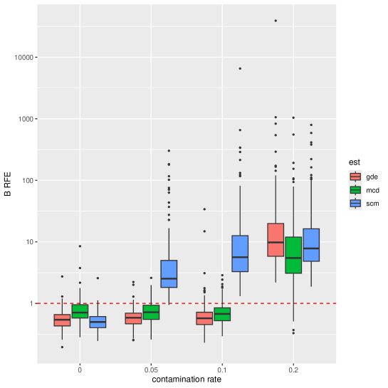
Figure 1: Logarithmic RFE for $\mathbf{B}$ as a function of the contamination rate for the default implementation (SCM) and the two robustified versions (MCD, GDE)

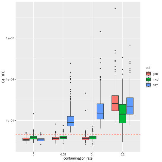
Figure 2: Logarithmic RFE for $\bm{\Sigma}_{\mathbf{e}}$ as a function of the contamination rate for the default implementation (SCM) and the two robustified versions (MCD, GDE)

For the evaluation of those robust variants of LLC, we have to apply them to data that we know the causal ground truth of. Unfortunately, there are only very few real-world datasets that satisfy this condition. And they are certainly not available with known contaminations and in amounts necessary for the statistical evaluations conducted here. That is why we confine ourselves to synthetic data. We will consider 200 randomly generated causal systems with five nodes each. The probability of an edge is set to 0.3, as is that of a confounder. For each model, we simulated six experiments, one is the purely observational experiment, joined by one singular perfect intervention experiment for each node. For each experiment, we create a sample of size 200, which will contain randomly generated contaminations of $\mathbf{x}$. For more details about the configurations, see our R implementation on GitHub (the repository will be made publicly available after the publication of the paper).

The three estimators considered are the LLC estimators $(\hat{\mathbf{B}},\hat{\bm{\Sigma}}_{\mathbf{e}})$ using for the estimation of $\mathbf{C}_{\mathbf{x}}^{k}$ the estimators SCM, MCD, and GDE. For the comparison we use the relative Frobenius error (RFE) as discussed in Section 3.5. First, we examine data without any contamination ($\varepsilon=0$) and record for all three estimators the median and MAD (Median Absolute Deviation), taken over the 200 random models, of the RFE. The result is given in Table 1. Next, the same procedure was applied to contamination rates $\varepsilon=0.05$ and $\varepsilon=0.1$ with the results in Table 2 and 3.

Table 1: Median and MAD of RFEs for $\varepsilon=0$

Estimator	$\hat{\mathbf{B}}$ RFE		$\hat{\bm{\Sigma}}_{\mathbf{e}}$ RFE
	Median	MAD	Median	MAD
SCM	0.50	0.15	0.38	0.11
MCD	0.71	0.27	0.55	0.17
GDE	0.54	0.17	0.43	0.12

Table 2: Median and MAD of RFEs for $\varepsilon=0.05$

Estimator	$\hat{\mathbf{B}}$ RFE		$\hat{\bm{\Sigma}}_{\mathbf{e}}$ RFE
	Median	MAD	Median	MAD
SCM	2.52	1.46	6.94	5.83
MCD	0.72	0.28	0.58	0.18
GDE	0.58	0.17	0.49	0.16

Table 3: Median and MAD of RFEs for $\varepsilon=0.1$

Estimator	$\hat{\mathbf{B}}$ RFE		$\hat{\bm{\Sigma}}_{\mathbf{e}}$ RFE
	Median	MAD	Median	MAD
SCM	5.63	4.72	35.02	42.86
MCD	0.68	0.24	0.54	0.18
GDE	0.57	0.20	0.48	0.17

We can see that, for the uncontaminated data, SCM has, in median, the least relative error and the robust versions follow with a small increase. For the data with the relatively small contaminations of $\varepsilon=0.05$ and $\varepsilon=0.1$, we already see a strong increase in the relative errors for SCM, while there is almost no change for MCD and GDE.

All the differences in the median values are highly significant w.r.t. Wilcoxon signed-rank test, thanks to the high number of random models, with even the largest p-value being less than $10^{-3}$. Thus, at least in this particular setting, GDE seems to be superior to MCD. To better see the dependence of the error on the contamination rate, we plotted the errors of the 200 models as dodged boxplots grouped by $\varepsilon$ and the estimators. For $\mathbf{B}$ see Figure 1, for $\bm{\Sigma}_{\mathbf{e}}$ see Figure 2. The horizontal red dashed line indicates the relative error of 1, i.e., everything above this line is only of very limited use. Note, that the y-axis is logarithmic. Up to the contamination rate of $\varepsilon=0.1$, the robustifications are clearly more robust than the baseline SCM, but starting with $\varepsilon=0.2$, even the robust implementations return data with RFE clearly above one.

6 Conclusion

Causality is nowadays successfully applied in many branches of science. To increase accuracy and widen the field of application, models allowing for feedback loops and hidden confounders need to be investigated more. We have focused on the LLC algorithm, which satisfies those two requirements. In particular, we have considered the robustness of LLC. The robustness of an estimator refers to its capability to remain mainly unperturbed by contamination of the measurement data with outliers. For the given scenario, we considered three different types of contamination. The robustness metric used here is the estimator’s BP. It was shown that the LLC estimator $(\hat{\mathbf{B}},\hat{\bm{\Sigma}}_{\mathbf{e}})$ is not robust, i.e., that its BP is zero. In a sense, it is even less robust than the covariance estimators it is based on. Finally, we have performed experiments investigating the effect of substituting robust covariance estimators into LLC. We focused on the robust estimators MCD and GDE, where we also provided an implementation for the latter. Those robust modifications of LLC are showing a clear improvement for lower contamination rates. In particular, in the considered scenario, the GDE-based LLC estimator outperforms the one based on MCD. In future work, we will investigate additional robustness metrics like those bound to the influence function approach.

The implementation of those extensions of LLC also contains a CCP version of GDE for the multivariate normal case. To improve reproducibility and encourage further research, the source code is made freely available on GitHub.

range

pages11 rangepages31 rangepages24 rangepages8 rangepages29 rangepages8 rangepages53 rangepages47 rangepages5 rangepages1 rangepages47 rangepages22

References

- [1] Vincent Arsigny, Pierre Fillard, Xavier Pennec and Nicholas Ayache “Log-Euclidean metrics for fast and simple calculus on diffusion tensors” In Magnetic Resonance in Medicine: An Official Journal of the International Society for Magnetic Resonance in Medicine 56.2 Wiley Online Library, 2006, pp. 411–421
- [2] Nihat Ay, Jürgen Jost, Hông Vân Lê and Lorenz Schwachhöfer “Information geometry” Springer, 2017
- [3] Ayanendranath Basu, Hiroyuki Shioya and Chanseok Park “Statistical inference: the minimum distance approach” CRC press, 2011
- [4] Stephan Bongers, Patrick Forré, Jonas Peters and Joris M Mooij “Foundations of structural causal models with cycles and latent variables” In The Annals of Statistics 49.5 Institute of Mathematical Statistics, 2021, pp. 2885–2915
- [5] P Laurie Davies “Asymptotic behaviour of S-estimates of multivariate location parameters and dispersion matrices” In The Annals of Statistics JSTOR, 1987, pp. 1269–1292
- [6] Ian L Dryden, Alexey Koloydenko and Diwei Zhou “Non-Euclidean statistics for covariance matrices, with applications to diffusion tensor imaging”, 2009
- [7] Frederick Eberhardt, Patrik Hoyer and Richard Scheines “Combining experiments to discover linear cyclic models with latent variables” In Proceedings of the Thirteenth International Conference on Artificial Intelligence and Statistics, 2010, pp. 185–192 JMLR WorkshopConference Proceedings
- [8] Shinto Eguchi and Osamu Komori “Minimum Divergence Methods in Statistical Machine Learning” Springer, 2022
- [9] Patrick Forré and Joris M Mooij “Markov properties for graphical models with cycles and latent variables” In arXiv preprint arXiv:1710.08775, 2017
- [10] Hironori Fujisawa and Shinto Eguchi “Robust parameter estimation with a small bias against heavy contamination” In Journal of Multivariate Analysis 99.9 Elsevier, 2008, pp. 2053–2081
- [11] Frank R Hampel, Elvezio M Ronchetti, Peter J Rousseeuw and Werner A Stahel “Robust statistics: the approach based on influence functions” John Wiley & Sons, 2011
- [12] Peter J Huber “Robust statistics” John Wiley & Sons, 2004
- [13] Antti Hyttinen, Frederick Eberhardt and Patrik O Hoyer “Causal discovery for linear cyclic models with latent variables” In Proceedings of the Fifth European Workshop on Probabilistic Graphical Models (PGM 2010), 2010, pp. 153–160 Citeseer
- [14] Antti Hyttinen, Frederick Eberhardt and Patrik O Hoyer “Learning linear cyclic causal models with latent variables” In The Journal of Machine Learning Research 13.1 JMLR. org, 2012, pp. 3387–3439
- [15] Olivier Ledoit and Michael Wolf “A well-conditioned estimator for large-dimensional covariance matrices” In Journal of multivariate analysis 88.2 Elsevier, 2004, pp. 365–411
- [16] Olivier Ledoit and Michael Wolf “Nonlinear shrinkage estimation of large-dimensional covariance matrices”, 2012
- [17] Ricardo A Maronna, R Douglas Martin, Victor J Yohai and Matías Salibián-Barrera “Robust statistics: theory and methods (with R)” John Wiley & Sons, 2019
- [18] Radford M Neal “On deducing conditional independence from d-separation in causal graphs with feedback (research note)” In Journal of Artificial Intelligence Research 12, 2000, pp. 87–91
- [19] Judea Pearl “Causality” Cambridge university press, 2009
- [20] Judea Pearl and Rina Dechter “Identifying independencies in causal graphs with feedback” In arXiv preprint arXiv:1302.3595, 1996
- [21] Jonas Peters, Dominik Janzing and Bernhard Schölkopf “Elements of causal inference: foundations and learning algorithms” The MIT Press, 2017
- [22] R R Core Team “R: A language and environment for statistical computing” Vienna, Austria, 2013
- [23] Peter J Rousseeuw “Multivariate estimation with high breakdown point” In Mathematical statistics and applications 8.283-297, 1985, pp. 37
- [24] Peter Spirtes, Clark N Glymour and Richard Scheines “Causation, prediction, and search” MIT press, 2000
- [25] Peter L Spirtes “Directed cyclic graphical representations of feedback models” In arXiv preprint arXiv:1302.4982, 1995
- [26] Valentin Todorov and Peter Filzmoser “An object-oriented framework for robust multivariate analysis” In Journal of Statistical Software 32, 2010, pp. 1–47
- [27] Alan L Yuille and Anand Rangarajan “The concave-convex procedure” In Neural computation 15.4 MIT Press, 2003, pp. 915–936