Metric Oja Depth, New Statistical Tool for Estimating the Most Central Objects

Abstract

The Oja depth (simplicial volume depth) is one of the classical statistical techniques for measuring the central tendency of data in multivariate space. Despite the widespread emergence of object data like images, texts, matrices or graphs, a well-developed and suitable version of Oja depth for object data is lacking. To address this shortcoming, in this study we propose a novel measure of statistical depth, the metric Oja depth applicable to any object data. Then, we develop two competing strategies for optimizing metric depth functions, i.e., finding the deepest objects with respect to them. Finally, we compare the performance of the metric Oja depth with three other depth functions (half-space, lens, and spatial) in diverse data scenarios.

[label1]organization=Department of Mathematics and Statistics,
University of Turku, country=Finland

1 Introduction

1.1 Background

Nowadays, data is being generated in high volumes, at high speeds, and with great diversity. In fact, it can be stated that with the advent of big data, we have entered a new phase of data analysis. A key aspect of modern data analysis is that we no longer deal exclusively with data existing in Euclidean spaces. Instead, data are currently taking on more complex formats, such as images, graphs, matrices, etc., all of which reside in non-Euclidean spaces and are collectively known as object data. Methods targeted towards object data, accordingly known as object data analysis or metric statistics [5], are currently bountiful in statistical literature, see, e.g., [6, 36, 38, 39].

As with any data, in order to achieve a better understanding of object data or to implement both simple and advanced machine learning algorithms on object data, it is essential to take some initial steps. These involve data cleaning and performing exploratory data analysis on the raw data. Exploratory data analysis can take various forms: calculating descriptive statistics, dimension reduction, detecting outliers etc. are all examples of exploratory data analysis. However, despite being straightforward and well-studied in the context of Euclidean data, these tasks can be surprisingly difficult in the context of object data, due to the lack of even basic mathematical operations such as addition. In this work, we focus on one of the most fundamental exploratory statistical tasks, location/mean/average estimation, in the context of object data. As our methodological tool of choice, we use depth functions, one of the lesser-known yet powerful and data-driven tools in exploratory data analysis, which we review next.

In statistical analysis, measuring the extent to which an observation is centralized or outlying within the data distribution plays a fundamental role. Subsequently, various statistical measures have been developed for this purpose and the history of this concept can be traced back to the early 1900s, to the concept of Mahalanobis distance. In fact, this distance serves as a classic method for quantifying how outlying a point is. In contrast to Mahalanobis distance and similar quantities, depth functions operate precisely in the opposite direction and measure the centrality, or depth, of a point with respect to a distribution (outlyingness and centrality are two contrasting concepts). In mathematical terms, for a point $x$ and a probability distribution $P$, a depth function $D$ assigns to $x$ a non-negative value $D(x,P)$ which quantifies the centrality of $x$ with respect to the probability distribution $P$. A higher depth value indicates that $x$ is located closer to the center of the data, while a lower depth indicates that this point is more outlying within the distribution. Going beyond the previous heuristic explanation, an ideal depth function is typically required to satisfy a certain collection of properties, see [40].

The foundation for depth functions was originally introduced in 1975 by Tukey who proposed his seminal half-space depth for multivariate data to rank observations and reveal features of the underlying data distribution [32]. Apart from the half-space depth, numerous depth functions for data in Euclidean space have been proposed. For instance, the convex hull peeling depth (onion depth) [1, 7] or Simplicial volume depth (Oja depth) [23] and several others, see Table 1 and the comprehensive addressing in [20].

Author	Year	Depth function	Has a metric version
Mahalanobis [18]	1936	Mahalanobis depth (distance)	No
Tukey [32]	1975	Half-space/location/Tukey depth	Yes [4]
Barnett, Eddy [1, 7]	1976, 1981	Convex hull peeling /onion depth	No
Liu; Zuo & Serfling [16, 40]	1992, 2000	Projection depth	No
Liu [15]	1990	Simplicial depth	No
Oja, Zuo & Serfling [23]	1983, 2000	Simplicial volume depth/Oja depth	Yes, in the current paper
Koshevoy & Mosler [14]	1997	Zonoid depth	No
Vardi & Zhang, Serfling [33, 29]	2000, 2002	Spatial depth	Yes [35]
Liu & Modarres [17]	2011	Lens depth	Yes [3, 12]
Yang & Modarres [37]	2018	$\beta$-skeleton depths	No

Table 1: List of depth functions and whether a metric version of them exists.

In recent years, object/metric versions of various depth functions (see the final column of Table 1) have been proposed to analyze samples of object data living in an arbitary metric space $(\mathcal{X},d)$. That is, these new depth functions are such that given an object $X\in\mathcal{X}$ and a distribution $P$ taking values in $\mathcal{X}$, the depth $D(X;P)$ describes how central the object $X$ is w.r.t. $P$, much in the same way as for the Euclidean depths earlier. Two key properties of these extensions is that (a) they depend on the data only through the metric $d$, making them applicable to any form of object data, regardless in which specific metric space they live, and (b) if $(\mathcal{X},d)$ is chosen to be a Euclidean space, then the original Euclidean version of the depth is recovered, showing that these metric depth functions are indeed “true” generalization of their classical counterparts. A metric version of the lens depth was developed in [3, 12], the metric half-space depth was proposed in [4] and the metric spatial depth in [35].

Most of the depth functions in Table 1, in particular all three that have object versions, are robust [19], meaning that their performance is not skewed by the presence of possible outliers. The same is not true for location estimation procedures in general. For example, the Fréchet mean [11] which is a generalization of the concept of average and a classical estimator of location for object data, is not robust, but is instead affected greatly by data outliers. Despite the popularity of Fréchet mean and similar tools, in this work we concentrate solely on robust methods. This is because object data is very diverse and recognizing any possible outliers in them can, as such, be very difficult. Hence, to ensure that our analyses stay reliable, we find it imperative to develop robust methods, which automatically protect us against outliers regardless of their exact type and whether we recognize them or not.

1.2 Our Contributions

As stated earlier, our focus in this work is on the robust location estimation of object data using depth functions. The main contributions of this work in this regard are as follows.

(i) We propose a new depth function for object data, the metric Oja depth. As with the metric generalizations of the other depth functions, the metric Oja depth is applicable to any object data and reverts back to the original Oja depth in Euclidean spaces. Like its competitors, it is also robust. Interestingly, the generalization process of Oja depth actually leads to several metric versions of it, indexed by a integer-valued dimension parameter $p$, see Section 3 for details, where we also derive several theoretical properties of the metric Oja depth that help interpreting it.

(ii) We study the robust estimation of the deepest point for object data samples. That is, given a sample $X_{1},\ldots,X_{n}$ of object data whose empirical distribution we denote by $P_{n}$, we aim to find the object $X\in\mathcal{X}$ which has the maximal depth value $D(X;P_{n})$. This deepest point serves as the analogue of sample mean for object data and has obvious uses in data analysis. Despite the fundamental nature of this problem, in the earlier works on metric depths it has been considered only by [4], and even they restricted to finding the optimum among the sample points $X_{1},\ldots,X_{n}$. As a more comprehensive approach, we propose using a genetic algorithm [13] along with a coordinate representation of the object data to estimate the deepest out-of-sample object. We demonstrate this with the metric Oja depth, but the proposed algorithm applies equally to any other metric depth function.

(iii) We conduct extensive simulation and real data comparisons between our proposed depth and all of its competitors from the literature on robust metric depths in estimating the deepest point in several object data scenarios. As one of our main questions of interest, we investigate how much the in-sample estimation can be improved by using the computationally expensive genetic algorithms to achieve out-of-sample estimation. In both simulation scenarios involving correlation matrices and points on hyperspheres, metric Oja depth performs best, with metric half-space depth showing the weakest performance but requiring less processing time. Applying the genetic algorithm to metric Oja depth further improved its performance.

We note that a prominent underlying theme in this work is the use of computationally intensive techniques to perform statistical inference for object data: E.g., since obtaining the null distribution for testing the equality of the deepest points of two distributions is not feasible, we use a permutation test to approximate this distribution in the absence of any distributional assumptions. Similarly, since depth functions are computationally complex and since a generic metric space does not carry enough structure for implementing standard optimization, we represent the objects as approximate coordinates and use genetic algorithms for heuristic optimization.

1.3 Contents

As shown in Table 1, three depth functions for object data have been developed earlier in the literature, which will be briefly introduced in Section 2. In Section 3, we provide a detailed explanation of a new metric depth function (two versions of that) developed in this research, outlining its features within theoretical framework. In Section 4, we evaluate and compare it with three other depth functions, using two simulation scenarios. We also apply a genetic algorithm to optimize out-of-sample error, and all experimental results are presented in this section. In Section 5, we further tested our metric depth function on real dataset to assess its performance in statistical inference, relying on computational techniques.Finally, future recommendations and conclusions are compiled in Section 6.

2 Review of existing metric depth functions

We next review the three existing depth functions for object data proposed in literature. We let $(\Omega,\mathcal{F},\mathbb{P})$ be a probability space and take $(\mathcal{X},d)$ to be a complete and separable metric space where our data (called hereafter “objects”) resides. Further, we let $P$ be a probability measure defined on the Borel sets of $\mathcal{X}$. Given a fixed, non-random object $x\in\mathcal{X}$, the metric depth functions answer the question “how central is the object $x$ with respect to the distribution $P$?”.

To tackle this quesition, [3, 12] proposed metric lens depth, defined as

$$D_{L}(x)\equiv D_{L}(x;P):=\mathbb{P}\left(d(X_{1},X_{2})>\max\left\{d(X_{1},x),d(X_{2},x)\right\}\right),$$

where $X_{1},X_{2}$ are independent random variables with the distribution $P$. We note that while the notation $D_{L}(x;P)$ is more transparent in the sense that it makes explicit the reference distribution $P$, we still use $D_{L}(x)$ in the sequel for conciseness, leaving $P$ implicit (but always clear from the context). Drawing an analogy from Euclidean statistics, $D_{L}(x)$ essentially gives the probability that the side corresponding to $X_{1},X_{2}$ is the longest in a “triangle” drawn using the objects $x,X_{1},X_{2}$. Intuitively, the probability is small (large) if $x$ is located far away from (close to) the bulk of the distribution $P$, making $D_{L}$ behave as expected from a depth function.

[4] gave a similar treatment to the classical half-space depth and defined the metric half-space depth as

$$D_{H}(x) =\inf_{{x_{1},x_{2}}\in\mathcal{X},\ d(x_{1},x)\leq d(x_{2},x)}\mathbb{P}(d(X,x_{1})\leq d(X,x_{2})).$$

The infimum is taken over pairs of objects $x_{1},x_{2}$ and every such pair divides the space $\mathcal{H}$ in two subsets (objects closer to $x_{1}$ than $x_{2}$ and vice versa). The depth $D_{H}(x)$ is defined to be the smallest possible probability mass of a subset produced in this way and containing the object $x$. As with the metric lens depth, it is easy to see that, for an outlying object $x$, it is easy to find a subset which contains $x$ but has very little $P$-probability mass, making $D_{H}(x)$ small.

A third metric depth was proposed in [35], who defined the metric spatial depth to be

where $X_{1},X_{2}\sim P$ are independent. The interpretation of $D_{S}(x)$ is trickier than for the previous two depths, but it essentially measures how likely $x$ and two random objects $X_{1},X_{2}$ are to yield equality in the triangle inequality. The depth takes values in $[0,2]$ and the value $0$ is reached if and only if the probability of equality is 1 and $x$ is never in the middle of the other two objects, whereas to reach the value $2$, $x$ must always reside between the two other objects. More details on interpreting the metric spatial are given in [35].

All previous metric depth functions revert to their classical counterparts when $(\mathcal{X},d)$ is taken to be an Euclidean space. They also share some key properties, which we summarize next. All three depths vanish at infinity meaning that, for objects far enough away from the bulk of the distribution $P$, the depth values approach zero. All three satisfy specific forms of continuity (small changes in $x$ entail small changes in the depth). Both $D_{L}$ and $D_{H}$ are invariant to data transformations that preserve the ordering of distances. The depths $D_{H}$ and $D_{S}$ are robust, the former in the sense of having a high breakdown point and the latter in the sense of having a bounded influence function. For these, and some other properties of the three depth functions, we refer the reader to the papers [3, 12, 4, 35].

Let $X_{1},\ldots,X_{n}$ denote a random sample of objects from the distribution $P$. Each of the three depth functions admits a natural sample counterpart where the reference distribution is taken to be $P_{n}$ the empirical distribution of the sample. In the sequel, we notate these sample versions as $D_{L,n},D_{H,n},D_{S,n}$. Thus, for example, the sample metric lens depth of $x$ is

$$D_{L,n}(x)\equiv D_{L}(x;P_{n}):=\frac{1}{n^{2}}\sum_{i=1}^{n}\sum_{j=1}^{n}\mathbb{I}\left(d(X_{i},X_{j})>\max\left\{d(X_{i},x),d(X_{j},x)\right\}\right).$$

We note that the computation of $D_{L,n}(x)$ and $D_{S,n}(x)$ is trivial, requiring just two loops over the sample, but finding $D_{H,n}$ is much more complicated due to the infimum. An approximative algorithm that we also use in this paper to compute the metric half-space depth is given in [4, Algorithm 1].

To complement this collection of metric depth functions, we next define a metric version of the Oja depth.

3 A new depth for object data

Before defining our novel depth concept, we first take a moment to motivate it. For any three objects $x_{1},x_{2},x_{3}\in\mathcal{X}$, we use the notation $L(x_{1},x_{2},x_{3})$ to denote the event that $d(x_{1},x_{3})=d(x_{1},x_{2})+d(x_{2},x_{3})$. To gain some intuition on this event, consider the following thought experiment: Assume that “transforming” an object $x\in\mathcal{X}$ to another object $y\in\mathcal{X}$ incurs a cost of $d(x,y)$, i.e., the farther apart (or, more different) the two objects are, the more costly the transformation. The triangle inequality can then be phrased as saying that a direct transformation from one object to another can never be more costly than going through a third object. Whereas, the event $L(x_{1},x_{2},x_{3})$ says that when transforming $x_{1}$ to $x_{3}$, such a “detour” through $x_{2}$ is actually free of cost. I.e., one may first transform $x_{1}$ to $x_{2}$ and then transform $x_{2}$ to $x_{3}$, with the same total cost as going directly from $x_{1}$ to $x_{3}$. For this to be possible, it is clear that $x_{2}$ has to reside (in some sense) “between” $x_{1}$ and $x_{3}$.

Following the above intuition, to simplify the exposition, we use in the following phrases such as “$x_{2}$ lies in between $x_{1}$ and $x_{3}$” to mean that the event $L(x_{1},x_{2},x_{3})$ holds. We also introduce the union event

$$U(x_{1},x_{2},x_{3}):=L(x_{1},x_{2},x_{3})\cup L(x_{2},x_{3},x_{1})\cup L(x_{3},x_{1},x_{2}).$$

Thus, $U(x_{1},x_{2},x_{3})$ means that at least one of $x_{1},x_{2},x_{3}$ is located in between the remaining two objects.

To put the previous ideas of in-betweenness to use, we next define two matrices which are intimately connected to them. Let first $x_{0},x_{1},x_{2},x_{3}\in\mathcal{X}$ be arbitrary objects. We denote by $B_{3}(x_{0},x_{1},x_{2},x_{3})$ the $3\times 3$ matrix whose $(k,\ell)$-element equals

$$\frac{1}{2}\left\{d^{2}(x_{0},x_{k})+d^{2}(x_{0},x_{\ell})-d^{2}(x_{k},x_{\ell})\right\}.$$

Moreover, we let $B_{2}(x_{0},x_{1},x_{2})$ denote the $2\times 2$ top left principal sub-matrix of $B_{3}(x_{0},x_{1},x_{2},x_{3})$. Our next result shows that the determinants of these two matrices contain interesting information on the relations between the four objects. The notation $|\cdot|$ in the result denotes the determinant.

Theorem 1.

• We have

  $$\left|B_{2}(x_{0},x_{1},x_{2})\right|\geq 0,$$

  where an equality is reached if and only if the event $U(x_{0},x_{1},x_{2})$ holds.

• We have

  $$\left|B_{3}(x_{0},x_{1},x_{2},x_{3})\right|\geq-4d^{2}(x_{0},x_{1})d^{2}(x_{0},x_{2})d^{2}(x_{0},x_{3}).$$ (1)

  If equality is reached in (1), then at least one of the events $L(x_{1},x_{0},x_{2})$, $L(x_{2},x_{0},x_{3})$, $L(x_{3},x_{0},x_{1})$ holds.

We now build measures of depth using the two matrices. Let $X_{1},X_{2},X_{3}\sim P$ be independent random objects and consider, for a fixed object $x\in\mathcal{X}$, the quantity

$$G_{3}(x)=\mathrm{E}\left[\left\{|B_{3}(x,X_{1},X_{2},X_{3})|+4d^{2}(x,X_{1})d^{2}(x,X_{2})d^{2}(x,X_{3})\right\}^{1/2}\right].$$

By Theorem 1, taking the square root is well-defined (we will prove that the expectation exists shortly). Theorem 1 also implies that $G_{3}(x)$ measures the outlyingness of the object $x$ with respect to the distribution $P$. That is, if $G_{3}(x)$ takes a small value, then the point $x$ must typically be located in between pairs of objects randomly drawn from $P$. To convert $G_{3}(x)$ into a measure of depth instead, we define

$$D_{O3}(x):=\frac{1}{1+G_{3}(x)},$$ (2)

where the subscript O refers to “Oja”, for reasons to be explained soon. As computing $D_{O3}(x)$ is costly due to the presence of the three random objects $X_{1},X_{2},X_{3}$, we consider as an alternative also the “bivariate” version,

$$D_{O2}(x):=\frac{1}{1+\mathrm{E}\left\{|B_{2}(x,X_{1},X_{2})|^{1/2}\right\}},$$ (3)

based on part (i) of Theorem 1. Intuitively, $D_{O2}(x)$ takes a large value if, for random $X_{1},X_{2}$ and the fixed object $x$, one of the three is typically in between the two others. Note that this does not yet guarantee that $x$ is deep with respect to $P$ as it is possible that $X_{1}$ (or $X_{2}$) is always the in-between point. However, our experiments later on show that, despite this uncertainty, $D_{O2}(x)$ manages to measure the depth of points very well in practice.

As mentioned above, our proposed object depth functions $D_{O2},D_{O3}$ are closely connected to the classical Oja depth [23] for multivariate data. For data residing in $\mathcal{X}=\mathbb{R}^{p}$, the Oja depth $D_{\mathrm{Oja},p}(x)$ of a point $x\in\mathbb{R}^{p}$ is defined as

$$D_{\mathrm{Oja},p}(x)=\frac{1}{1+\mathrm{E}\{V(x,X_{1},\ldots,X_{p})\}},$$

where $X_{1},\ldots,X_{p}\sim P$ are i.i.d. and $V(x,X_{1},\ldots,X_{p})$ denotes the hypervolume of the simplex in $\mathbb{R}^{p}$ having the vertices $x,X_{1},\ldots,X_{p}$. The intuitive idea behind $D_{\mathrm{Oja},p}$ is that outlying points $x\in\mathbb{R}^{p}$ typically lead to elongated simplices with large volumes, yielding small depths. The following result shows that when our data live in an Euclidean plane, then $D_{O2}$ and $D_{\mathrm{Oja},p}$ exactly coincide.

Theorem 2.

Let $\mathcal{X}=\mathbb{R}^{2}$ and $d$ be the corresponding Euclidean distance. Then we have $D_{O2}(x)=D_{\mathrm{Oja},2}(x)$ for all $x\in\mathbb{R}^{2}$.

In Theorem 2, both $D_{O2}$ and $D_{\mathrm{Oja},2}$ are understood to be computed with respect the same probability distribution $P$. At this point it is important to realize that there is a fundamental difference between the two concepts. Namely, Oja’s original intention was that, if the data resides in $\mathbb{R}^{p}$, then the version $D_{\mathrm{Oja},p}$ of the Oja depth should be used (instead of, say $D_{\mathrm{Oja},2}$ or $D_{\mathrm{Oja},p+1}$). In other words, the definition of the Oja depth depends non-trivially on the dimension $p$ of the space. Whereas, for our proposed depth $D_{O2}$, its underlying idea is that it can be used in any metric space, the definition staying unchanged. In particular, one can compute $D_{O2}$ for data in $\mathbb{R}^{p}$ (using the definition in (3)) and, from a geometric viewpoint, this corresponds to computing the average area of a 2-simplex defined by $x\in\mathbb{R}^{p}$ and $X_{1},X_{2}$ drawn i.i.d. from $P$.

For $D_{O3}$ the connection to the original Oja depth is not as transparent as for $D_{O2}$, as shown next.

Theorem 3.

Let $\mathcal{X}=\mathbb{R}^{3}$ and $d$ be the corresponding Euclidean distance. Then,

$$D_{\mathrm{Oja},3}(x)=\frac{1}{1+\mathrm{E}[|B_{3}(x,X_{1},X_{2},X_{3})|^{1/2}]}.$$

Comparison of Theorem 3 to (2) reveals that, in the three-dimension Euclidean space, $D_{O3}$ and $D_{\mathrm{Oja},3}$ are equivalent apart from the extra term $4d^{2}(x,X_{1})d^{2}(x,X_{2})d^{2}(x,X_{3})$. In fact, Lemma 6 in A shows that, for Euclidean data we always have $|B_{3}(x,X_{1},X_{2},X_{3})|\geq 0$, meaning that the adding of the “correction” term $4d^{2}(x,X_{1})d^{2}(x,X_{2})d^{2}(x,X_{3})$ is actually not needed in this case (to make the square root well-defined). This also means that the smallest possible values of $G_{3}(x)$ (i.e., the largest possible depths $D_{O3}(x)$) cannot be reached in Euclidean spaces as in them $|B_{3}(x,X_{1},X_{2},X_{3})|$ is always non-negative. Intuitively, this is because Euclidean spaces are too “structured” and more centrally located point configurations can be achieved in non-Euclidean geometries, see Section 3.2 in [35] for an example and a similar phenomenon.

We next establish a few key properties of $D_{O2}(x)$ and $D_{O3}(x)$, beginning with a moment condition that guarantees their existence.

Theorem 4.

Assume that, for some $a\in\mathcal{X}$, we have $\mathrm{E}\{d(X,a)\}<\infty$. Then $D_{O2}(x)$ and $D_{O3}(x)$ exist as well-defined.

Several notes about Theorem 4 are in order: (i) By “well-defined”, we mean that the expected values used to compute $D_{O2}(x)$ and $D_{O3}(x)$ are finite. (ii) The condition $\mathrm{E}\{d(X,a)\}<\infty$ is analogous to requiring a univariate random variable to have a finite mean, making Theorem 4 perfectly in line with the results for classical Oja depth that also require the existence of first moments, see [21, 10]. (iii) Requiring the existence of the first moment is quite a mild condition and less than many standard methods require. Indeed even the Frechét mean already requires the existence of second moments. (iv) The choice of $a$ in Theorem 4 is completely arbitrary as, if the condition $\mathrm{E}\{d(X,a)\}<\infty$ holds for some $a$, then, by the triangle inequality, it holds for all $a\in\mathcal{X}$.

Below we say that a sequence of objects $x_{n}\in\mathcal{X}$ is divergent if there exists $a\in\mathcal{X}$ such that $d(x_{n},a)\rightarrow\infty$ when $n\rightarrow\infty$. Intuitively, a divergent sequence of objects is such that it moves “towards infinity” eventually getting arbitrarily far from any fixed object. It is clear that such sequences do not exist in every metric space, for example, on the unit sphere equipped with the arc length metric. Divergent sequences make for a natural model for outlying observations. And since we claim $D_{O3}(x)$ to measure the centrality of the object $x$, it is intuitive to require that $D_{O3}(x_{n})$ goes to zero for any divergent sequence $x_{n}$. This is formalized in our next result.

Theorem 5.

Assume that, for some $a\in\mathcal{X}$, we have $\mathrm{E}\{d^{2}(X,a)\}<\infty$. Let $x_{n}$ be a divergent sequence of points in $\mathcal{X}$. Then, $D_{O3}(x_{n})\rightarrow 0$ as $n\rightarrow\infty$.

The second moment condition in Theorem 5 is used to avoid certain pathological behavior, see the proof of the result. Note also that an analogous result for $D_{O2}(x)$ cannot be derived. This is because, as evidenced in Theorem 1, $D_{O2}(x)$ does not characterize centrality in the same sense as $D_{O3}(x)$ and it is possible to have outlying objects that still obtain a large value for $D_{O2}(x)$. As an extreme example of this, if $(\mathcal{X},d)$ is the one-dimensional Euclidean space, then it is simple to check that $D_{O2}(x)=1$ for all points $x\in\mathbb{R}$.

Finally, note that both $D_{O2}$ and $D_{O3}$ admits the natural sample counterparts, $D_{O2,n}$ and $D_{O3,n}$, computed exactly as (3) and (2), but with the expectations replaced with double or triple sums over the sample, respectively. In the next section, we apply these sample depths in various object data scenarios to showcase their usefulness.

4 Simulation examples

4.1 In-sample optimization

Throughout the examples, we abbreviate the used depth functions as follows: MOD2, MOD3 refer to the two versions of the metric Oja depth, MHD denotes the metric half-space depth [4], MLD the metric lens depth [3, 12], whereas MSD refers to the metric spatial depth [35]. In our first experiment we evaluate and compare the performances of our proposed MOD2 and MOD3 with their three competitors from the literature, MHD, MLD, and MSD, using simulated scenarios. We do this in the context of location estimation. Given a sample $X_{1},\ldots,X_{n}\in\mathcal{X}$ from a distribution $P$, each sample depth function $D_{n}$ is used to determine an in-sample estimate of the deepest object, i.e., $\hat{\mu}:=X_{i_{0}}$ where $i_{0}=\mathrm{argmin}_{i=1,\ldots,n}D_{n}(X_{i})$. The methods are then compared based on the averages, over 200 replications, of the estimation errors $d(\hat{\mu},\mu)$ where $\mu\in\mathcal{X}$ is the true deepest object of the data-generating distribution $P$. In addition to the average error, we compare also the average computation times of the depths.

4.1.1 Correlation matrix dataset

In our first simulation, we consider the Riemannian manifold $(\mathcal{X},d)$ of $p\times p$ correlation matrices as the data space, where $d(X_{1},X_{2})=\|\mathrm{Log}(X_{1}^{-1/2}X_{2}X_{1}^{-1/2})\|_{F}$ is the affine invariant Riemannian metric, see [2]. The selection of this specific form of data is motivated by several key considerations. Firstly, correlation matrices are a “non-trivial” form of object data in the sense that they do not admit a simple, interpretable transformation to an Euclidean space (c.f. compositional data and the ilr-transformation, see [24]). Secondly, many datasets, especially in fields such as neuroscience, are structured as correlation matrices. A prime example is given by brain connectivity matrices [30] where each correlation describes the strength of connection between two brain regions.

To generate a sample $X_{1},\ldots,X_{n}$ of random correlation matrices, we first generated random $p\times p$ variance-covariance matrices $S_{i}$ and then scaled them in the usual way as $X_{i}:=\mathrm{diag}(S_{i})^{-1/2}S_{i}\mathrm{diag}(S_{i})^{-1/2}$. The $S_{i}$ were generated using the eigendecomposition form $S_{i}:=U_{i}D_{i}U_{i}^{\prime}$, where $U_{i}$ is a random orthogonal matrix and $D_{i}$ is a diagonal matrix with all positive diagonal elements, independent of $U_{i}$. We generated $U_{i}$ as uniformly random using the function rorth in the R-package ICtest [22], see [31] for details. This choice (uniform randomness of $U_{i}$) ensures that, in the end, we have covariance matrices whose eigenvectors are equally likely to point in any direction, implying that the true deepest covariance matrix of the distribution of $S_{i}$ is proportional to the identity matrix, i.e., $C\times I_{p}$, for some constant $C>0$. As the correlation matrices $X_{i}$ are obtained from the $S_{i}$ by scaling the diagonal elements to unity, this implies that the true deepest object for the $X_{i}$ is $\mu=I_{p}$. The diagonal matrices $D_{i}$ were generated as follows

where $\mathcal{N}(\nu,1)$ denotes a normal random variable with mean $\nu$ and unit variance. The parameter $\nu$ was determined as follows: each $X_{i}$ had the probability $\varepsilon>0$ of being deemed an “outlier”, in which case we took $\nu=3$, whereas the remaining $1-\varepsilon$ proportion of the data (the bulk) used $\nu=0$. Note that both the bulk and the outliers share the same true deepest object (identity matrix) but the high variance of the outliers is expected to make the estimation more difficult when $\varepsilon$ is increased.

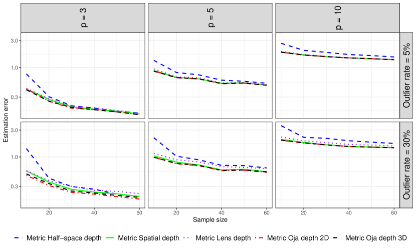
Figure 1: The average estimation errors for each of the five metric depth functions in the correlation matrix simulation. The scale of the $y$-axis is logarithmic.

Having fixed $\nu$, the simulation has three parameters, the contamination proportion $\varepsilon=0.05,0.30$, dimension $p=3,5,10$ and sample size $n=10,20,30,40,50,60$, leading to a total of 36 different cases. Note that $n$ was deliberately chosen as low, since object data scenarios typically have much smaller sample sizes than in standard Euclidean data analysis. The results of this simulation are shown in Figure 1, grouped by $\varepsilon$ and $p$. As is clearly observed, in all six subfigures, as the sample size $n$ increases, the estimation error gradually decreases. These results provide evidence that the estimators are consistent and adhere to the law of large numbers. Moreover, the complexity of the data space grows as the dimension $p$ of the matrices increases, leading to a decline in accuracy and meaning that the estimation error experiences an upward trend from $p=3$ to $p=10$. It is worth noticing that increasing the percentage of outliers from $5\%$ to $30\%$ did not lead to significant changes in the results, and the estimation error is only slightly higher when we have more outlier points, showing that the performance of the estimators remains stable, indicating that the estimators are indeed robust.

An alternative version of Figure 1 where the results are shown relative to MSD is presented in B and allows for better comparing the results of the methods within one subplot. Moving to a more detailed analysis, it can be seen that in all cases, MOD2 (red dashed-dotted line) and MOD3 (black dashed line) demonstrated the best performance, respectively, while MHD (blue dashed line) showed the weakest performance. The metric spatial depth was the third most efficient method and close to the Oja depths in performance. From the timing results given in Figure 2 we observe that neither $p$ nor $\varepsilon$ affect the running time. This is because the distance matrix $D$ from which the depths are computed remains an $n\times n$ matrix for any values of $p$ and $\epsilon$, meaning that only the increase in sample size has caused the increase in computation time in the plot. This effect is typical in object data analysis where most methods operate solely on the inter-object distances. Additionally, MOD2 and MOD3 have a relatively high time cost (the computational complexity of the metric Oja depth 3D is asymptotically of the order $\mathcal{O}(n^{4})$), meaning that these depths essentially offer improved performance at the cost of speed. Whereas, MSD shows the best performance in terms of time efficiency.

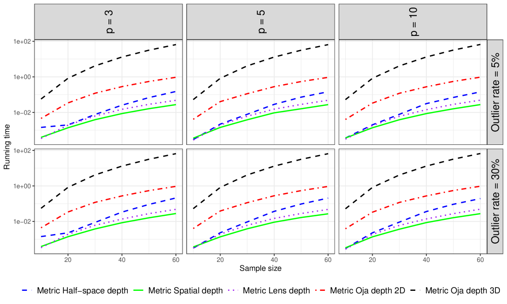
Figure 2: The running times (in seconds) of each metric depth function in the correlation matrix simulation. The scale of the $y$-axis is logarithmic.

4.1.2 Hypersphere dataset

In this experiment, we generated samples of points on a $p$-dimensional unit hypersphere $\mathcal{X}$, which is a higher-dimensional generalization of the unit circle in $\mathbb{R}^{2}$. As a metric $d$, we used the usual arc length distance. Each point $X_{i}$ was simulated by generating the $p$-dimensional random vector $Z_{i}$ from $\mathcal{N}_{p}(\lambda 1_{p},I_{p})$, where $1_{p}$ is a vector of ones and $\lambda\neq 0$, and then taking $X_{i}:=Z_{i}/\|Z_{i}\|$. By symmetry, this strategy leads to the deepest object always being equal to $\mu=\mathrm{sign}(\lambda)(1/\sqrt{p})1_{p}$ and the absolute value of the parameter $\lambda$ controls the spread of the points; the larger the value of $|\lambda|$, the more closely the points are concentrated around the deepest point. For the outliers we used $\lambda=-1$ and for the bulk $\lambda=5$, meaning that the two distributions have their deepest points on the opposite sides of the hypersphere, see Figure 3 for an illustration in the case $p=3$.

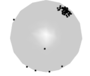
(a) $\lambda_{bulk}=5\quad,\quad\lambda_{outlier}=-1$

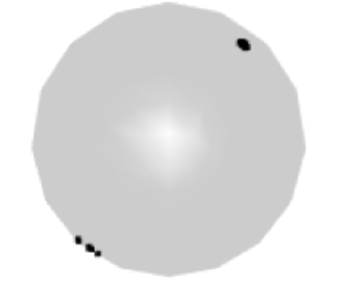
(b) $\lambda_{bulk}=40\quad,\quad\lambda_{outlier}=-10$

Figure 3: A visualization of the distribution of points generated with different $\lambda$-values on a 3-dimensional hypersphere, i.e., when $p=3$: ($a$) represents the case where $\lambda$ for the bulk is 5, and the $\lambda$ for the outliers is -1 and ($b$) shows the case where $\lambda$ for the bulk is 40, and the $\lambda$ for the outliers is -10. Essentially, the larger $\lambda_{bulk}$ is, the easier it becomes for depth functions to estimate deepest point.

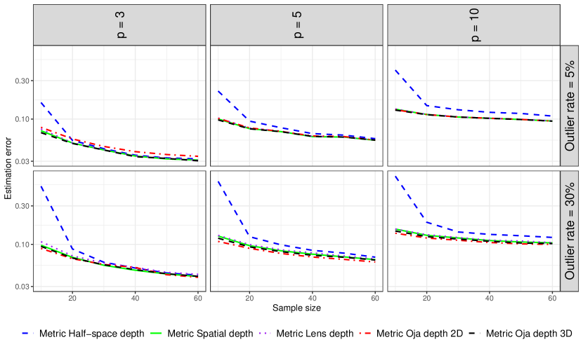
Figure 4: The average estimation errors for each of the five metric depth functions in the hypersphere simulation. The scale of the $y$-axis is logarithmic.

The simulation thus has three parameters, $\varepsilon$, $p$, $n$, and we use for them the same values as in the earlier simulation. As shown in Figure 4 and its relative version presented in B, the performance of each metric depth function on the hypersphere dataset is very similar to their performance on the correlation data. However, there is a slight difference: when the rate of outliers increases, MOD2 performs better than MOD3. This difference was not as noticeable in the earlier correlation data and indicates that MOD2 tolerates outliers better than MOD3. We have omitted the timing results for the sphere simulation as they were visually almost identical to Figure 2, again demonstrating that in object data analysis the actual data type rarely affects computational details.

Based on the results of the two simulation experiments, we make two recommendations. If $n$ is large and computational time is at a premium, MSD is an attractive choice, considering it did not have a large difference in performance compared to MOD2 and MOD3 in Figure 1. Whereas, if $n$ is small or computational time is not an issue, then the most accurate estimation can be expected from MOD2 and MOD3, which gave the best performance in all scenarios considered. Finally, we note that, while the absolute differences between the leading methods are not that large, even a small decrease in the error can be significant in the context of the very small sample sizes encountered commonly with object data. In the next section we then show how more drastic improvements can be achieved with the expense of added computational resources.

4.2 Out-of-sample optimization

The in-sample optimization studied in the previous section might come across as an overly naive approach, but in many metric spaces it is the best one can do, the lack of Euclidean structure preventing the use of standard optimization algorithms. However, despite being non-Euclidean, some metric spaces admit coordinate representations/encodings in Euclidean spaces, e.g., unit spheres (stereographic projection), the positive definite manifold (Cholesky decomposition) and the space of $L_{2}$-functions (Karhunen-Loève expansion, assuming we truncate it). In these cases, the full Euclidean non-linear optimization machinery can be brought forth to find the deepest point.

To formalize the earlier, assume that there exists a bijective map $f:\mathcal{X}\to\mathcal{S}$ where $S\subseteq\mathbb{R}^{q}$ for some $q$. Then, the problem of finding the deepest object of a sample $X_{1},\ldots,X_{n}\in\mathcal{X}$ can be formulated as

$$\max_{v\in\mathcal{S}}D_{n}(f^{-1}(v)),$$ (4)

where $D_{n}$ is some metric depth function w.r.t. the sample and $v$ is an Euclidean vector. After finding the optimizer $v_{0}$, it can be mapped to $\mathcal{X}$ simply as $f(v_{0})$. Since the map $v\mapsto D_{n}(f^{-1}(v))$ is highly non-convex, the use of any standard optimizer, e.g., gradient descent, is likely infeasible. As such, we propose using a genetic algorithm (GA) for the purpose. Genetic algorithm is a non-linear optimization procedure where a “population” of solution candidates is evolved through multiple generations. The “fittest” candidates (i.e., the ones having the largest value for the objective function) of each generation are combined and randomly mutated in order to produce the next, hopefully still fitter generation, see [13] for details and a systematic literature review on GA. Genetic algorithms have been earlier applied in descriptive statistical methodology particularly in the context of projection pursuit, see, e.g., [8].

We employed here the implementation provided by the R-package GA [27, 28], configuring the algorithm with the following tuning parameters: a population size of 500 and a maximum of 30 iterations. The initial values were set using the principal component representations of the top five in-sample deepest points. Additionally, the search space was defined with a width of 0.10 for each dimension. Even with a reasonable amount of iterations, the resulting computational cost of GA is very heavy and, for demonstration purposes, we apply the GA in this example only to a single depth function, chosen to be MOD2 now. To further alleviate computational burden, we apply a dimension reduction via PCA to the representations in the space $\mathcal{S}$ to map them to an $r$-dimensional space with $r\ll q$. As training data for the dimension reduction, we use the images $f(X_{1}),\ldots,f(X_{n})$ of the sample. As part of the next simulation, we investigate the trade-off between computational burden and accuracy related to the choice of $r$. As data, we generate a sample of correlation matrices similarly as described in Section 4.1, meaning the $(\mathcal{X},d)$ is now the manifold of positive definite matrices having unit diagonal. We define the map $f$ such that $f(X_{i})$ is the vector of length $p(p+1)/2$ containing the non-zero elements in the Cholesky decomposition of $X_{i}$. As the genetic algorithm can produce solutions lying outside of the set $\mathcal{S}$ (that is, solutions which are covariance matrices, but not correlation matrices), we manually scale the final optimizer $f(v_{0})$ into a proper correlation matrix.

In this simulation, the matrix dimension $p$ was set to 5, and the contamination proportion $\varepsilon$ was fixed to 30%. The sample size, as in previous simulations in Sections 4.1.1 and 4.1.2, was considered to be $n=10,20,30,40,50,60$. A new parameter introduced in this simulation was the number of principal components, determined by three proportions $\mathrm{PEL}=0.25,0.5,0.75$ of the $f(X_{i})$ vector length. Thus, the number of principal components is $r=\mathrm{PEL}(p(p+1))/2$. The whole simulation was repeated 200 times and in each replication the aforementioned 18 cases were considered. Moreover, we computed the in-sample estimator of the deepest object as a rival method to compare its performance to GA as well. As observed in Figure 5 (left), the use of a genetic algorithm combined with dimension reduction (represented by the purple, green, and blue lines, which correspond to 0.75, 0.5, and 0.25 of the length of the Cholesky decomposition vector considered as the number of principal components, respectively) has significantly contributed to reducing the estimation error compared to using only thein-sample estimator, which is indicated by the red line.

The next noteworthy point is that using a larger number of principal components will yield the best results. However, if the dimension reduction is too significant (e.g., 0.25), it may result in the loss of substantial useful information from the data. On the other hand, if the reduction is moderate (e.g., 0.5), the necessary information might be retained in some cases, while in others, important information could mistakenly be discarded. Additionally, considering the time cost, as shown in the right side of Figure 5, despite the substantial computational burden imposed by using genetic algorithms, we observe that with increasing sample size, even without using GA, the in-sample estimator tends to follow a similar trend.

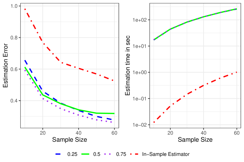
Figure 5: Left: The average estimation errors for each of the functions in the GA simulation. All methods are based on MOD2. Right: The running times (in seconds) of each function in the GA simulation. The scale of the y-axis is logarithmic.

5 Real data example

In this section, we aim to evaluate the performance of the proposed depth functions using real data. The secondary aim of this experiment is to demonstrate how the depth functions, whose analytically complex form prevents theoretical inferential results, can still be used for statistical inference via relying on computational techniques. For this purpose, the Canadian Weather data were utilized, see [26]. This data set contains the average daily temperatures of 35 Canadian provinces over a year and, as is standard, we smoothed them into periodic functional data $X_{i}(t)$, $i=1,\ldots,35$, $t=0,\ldots,365$, using a 100-element Fourier basis in the R-package fda [25].

The 35 stations each belong to one of four geographic regions: Arctic, Continental, Pacific, and Atlantic. Based on the geographic locations of these regions, we hypothesize that the temperatures in the coastal areas, i.e., the Atlantic and Pacific, should be similar, while the temperatures in the northern (Arctic) and central southern (Continental) regions of Canada should be colder and differ from the previous two. This is visually confirmed in Figure 6 (left), where the Atlantic and Pacific regions are generally warmer throughout the year, while the Arctic and Continental regions are colder. We thus divide the $n=35$ stations into two groups — the eastern and western coastal areas, and the northern and central southern areas — and our research question is: Is there a significant difference in the typical temperature curves between these two groups?

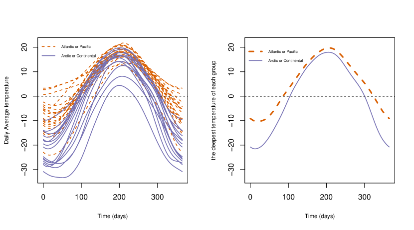
Figure 6: Left panel: The yearly average temperatures for $n=35$ Canadian weather stations, divided into two groups according to geographical location. Right panel: the deepest in-sample curves in each group, as determined by MOD3 with $L_{2}$-distance as the metric.

We next study this question by treating the curves as objects in a metric space $(\mathcal{X},d)$ where $d$ is the $L_{p}$-distance for some value of $p\in[1,\infty]$, implemented in R in the package fda.usc [9]. According to Figure 6 (right), which shows the deepest in-sample curves of these two groups as determined by MOD3 with $L_{2}$-distance as the metric, it appears that there is indeed a difference in their yearly behaviours. However, to confirm this, we next conduct a permutation test for determining whether the difference in the deepest curves in the two groups is statistically significant. Letting $f_{1},f_{2}\in\mathcal{X}$ denote the deepest in-sample curves of the two groups, we use as our test statistic the $L_{p}$-distance between them, $t=d(f_{1},f_{2})$. To simulate the distribution of $t$ under the null hypothesis (i.e., assuming no difference between the two groups), we randomly permute the group labels of the $n=35$ curves and compute the test statistic value. This reshuffling was done a total of 5000 times, yielding $t^{*}_{1},\ldots,t^{*}_{5000}$, using which the $p$-value of the test is computed as $\#\{t\leq t^{*}_{i}\}/5000$.

The resulting $p$-values for the five different depths and $L_{p}$-metrics with $p=1,2,3,4,5,10,20,\infty$, are shown in Figure 7 (left). These metrics measure distinct forms of difference between the curves (i.e., the higher $p$ is, the more the metric $L_{p}$ focuses on local properties), but all of them agree that there is a difference between the groups at the significance level $0.05$. Similarly, no quantitative differences are observed between the five depths, although MLD and MHD appear the least stable with respect to the change of $p$ (assuming that the null hypothesis is indeed false). The most consistent performance across $p$ is given by MOD3.

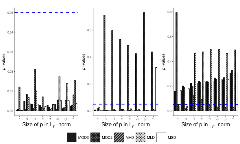
Figure 7: The $p$-value result of permutation test for each depth function across different choices of $p$ in $L_{p}$-norm. The test is at level $\alpha$ = 0.05, indicated by the horizontal dashed-line. Left: original data. Middle: 7 swaps. Right: 12 swaps.

We next take the previous result of no differences as a ground truth and continue the experiment by (a) contaminating the original data set, and (b) performing the same test for the contaminated data set and observing which of the depth-metric combinations still let us obtain the correct conclusion (no differences). This experiment thus mimics the practical scenario where the data has been partially wrongly recorded. To perform the contamination, we randomly select $k$ stations and swap their labels (a group 1 station becomes group 2 station and vice versa), using two different choices, $k=7,12$.

The resulting permutation test $p$-values for these data are shown in Figure 7 (middle and right) and show that under medium contamination (7 out of 35 stations mislabeled), all depths except MOD2 continue to yield the correct decision. The underlying reason for this is that MOD2 is not a “true” depth function and does not necessarily measure centrality of its input object, see the discussion after formula (3). Whereas, under high contamination (12 out of 35 stations mislabeled) only MHD continues to correctly identify the groups as distinct (for the majority of $L_{p}$-norms). This is quite a good result as having 1/3 of the data mislabeled makes for an exceedingly difficult case, and attributable to the excellent robustness properties of MHD, see Section 3.3. in [4]. We next inspect the stability of the $p$-values with respect to the choice of the norm; in practice one typically chooses only one norm to work with and, in this sense, having the same decision for all norms is practically desirable. Of the depths MLD is clearly the least stable, with MOD2 also exhibiting some unstability (but still uniform decisions across all norms). The three other depths are more or less stable. Finally, we note that the performance of MOD3 and MSD is almost equal in all scenarios, with the minor exception of the $L_{\infty}$-case under medium contamination. In this sense, the results align with the simulation studies in Section 4.1 where MSD was always almost as good as MOD3.

6 Conclusions

This study introduced two new versions of the Oja depth in non-Euclidean spaces and compared their performance with three established metric depth functions. Initially, we compared the performance of these five metric estimators using two simulated datasets. Under these two simulation scenarios, MOD2 and MOD3 (the two new proposed depth functions) respectively achieved the best performance, although both were more time-consuming than the others. Moreover, the weakest performance was observed with the MHD. Among the remaining functions, only MSD demonstrated relatively good performance after MOD2 and MOD3, and was also the fastest, potentially making it a useful alternative for practical applications.

Next, for the first time a metaheuristic approach (Genetic Algorithm) was employed to evaluate the introduced estimators on an unseen sample. To save time, we only selected the MOD2 and used PCA (Principal Component Analysis) for dimensionality reduction. With the genetic algorithm, we observed a substantial improvement in the selected estimator’s performance across all sample sizes, from 10 to 60, compared to its performance without genetic algorithm. However, a notable downside is that genetic algorithm incurs a significant computational cost.

Finally, we used a real data (Canadian weather dataset) to compare the metric depth functions’ effectiveness in a statistical two-sample location hypothesis test. Initially, we examined the original data, divided into two geographically distinct groups, and used five metric depth functions (for different $p$ in $L_{p}$ norm) to find the distance between the two deepest objects in each group. Among all methods, MOD3 consistently produced the most stable results across p-values, while MLD and MHD were the least stable. For further evaluation, we intentionally misassigned a subset of data points between groups and repeated the permutation test. In this case, MOD2 was the only one to produce incorrect results, while the others remained accurate. However, when the rate of misassignments increased, MHD became the only method to maintain correct results.

In conclusion, by following the recommendations we provide, this study can be further improved in the future. As mentioned, despite the promising performance of the two new metric depths presented here, both functions involve a significant time cost. By using partial U-statistics to randomly choose which elements to include in the triple sum in the sample version of (2), the speed of MOD3 computation can be enhanced. Additionally, to evaluate and compare the methods more clearly, the relative form of estimation error could be used instead of the absolute one. Another important point that could impact future results is the process of selecting and setting appropriate values for the hyper-parameters (take initial values as an example) used in the genetic algorithm. In future research, by developing meta-heuristic algorithms tailored to non-Euclidean spaces, it will be possible to reduce or eliminate the need for repetitive transformations between different spaces.

Acknowledgments

The work of both VZ and JV was supported by the Research Council of Finland (Grants 347501, 353769).

Supplementary materials

All computational parts were implemented in the R programming language and are accessible through this GitHub link.

Appendix A Proofs of theoretical results

Proof of Theorem 1.

Let $b_{k\ell}$ denote the $(k,\ell)$-element of the matrix $B_{3}(x_{0},x_{1},x_{2},x_{3})$. From the proof of Theorem 1 in [34] we have that $|b_{k\ell}|\leq d(x_{0},x_{k})d(x_{0},x_{\ell})$. Moreover, the two extremes satisfy: (i) $b_{k\ell}=d(x_{0},x_{k})d(x_{0},x_{\ell})$ if and only if either $d(x_{0},x_{k})=d(x_{0},x_{\ell})+d(x_{\ell},x_{k})$ or $d(x_{0},x_{\ell})=d(x_{0},x_{k})+d(x_{k},x_{\ell})$. (ii) $b_{k\ell}=-d(x_{0},x_{k})d(x_{0},x_{\ell})$ if and only if $d(x_{k},x_{\ell})=d(x_{k},x_{0})+d(x_{0},x_{\ell})$. Thus, in particular, $|b_{k\ell}|=d(x_{0},x_{k})d(x_{0},x_{\ell})$ if and only if $U(x_{0},x_{k},x_{\ell})$ is true.

Take first $p=2$. In this case $|B_{2}(x_{0},x_{1},x_{2})|=d^{2}(x_{0},x_{1})d^{2}(x_{0},x_{2})-b_{12}^{2}$. By the preceding paragraph, $|B_{2}(x_{0},x_{1},x_{2})|\geq 0$ where equality is reached precisely under the condition claimed in the theorem statement.

For $p=3$, Sarrus’ rule and the previous inequalities give

$$\begin{split}|B_{3}(x_{0},x_{1},x_{2},x_{3})|&=b_{11}b_{22}b_{33}+2b_{12}b_{23}b_{31}-b_{11}b_{23}^{2}-b_{22}b_{31}^{2}-b_{33}b_{12}^{2}\\ &\geq-2b_{11}b_{22}b_{33}+2b_{12}b_{23}b_{31}.\end{split}$$ (5)

Now, $2b_{12}b_{23}b_{31}\geq-2b_{11}b_{22}b_{33}$, establishing the claimed inequality. Moreover, equality is reached in $2b_{12}b_{23}b_{31}\geq-2b_{11}b_{22}b_{33}$ if and only if either (a) all of $b_{12},b_{23},b_{31}$ reach their lower bounds given in the first paragraph of the proof, or (b) two of $b_{12},b_{23},b_{31}$ reach their upper bounds and one reaches their lower bound. As reaching the lower bound for $b_{ij}$ implies that the corresponding event $L(x_{i},x_{0},x_{j})$ holds, the proof is concluded.

∎

We omit the proofs of Theorems 2 and Theorems 3 as they follow instantly from the more general Lemma 6 presented below.

Lemma 6.

The Oja depth $D_{\mathrm{Oja},p}(x)$ of a point $x\in\mathbb{R}^{p}$ can be written as

$$\frac{1}{1+\mathrm{E}[\{C(x,X_{1},\ldots,X_{p})\}^{1/2}]},$$ (6)

where

$$C(x,X_{1},\ldots,X_{p})=\left|\begin{pmatrix}k_{11}&k_{12}&\dots&k_{1p}\\ k_{21}&k_{22}&\dots&k_{2p}\\ \vdots&\vdots&\ddots&\vdots\\ k_{p1}&k_{p2}&\dots&k_{pp}\end{pmatrix}\right|,$$

and

$$k_{mn}=-\frac{1}{2}(\norm{X_{n}-X_{m}}^{2}-\norm{X_{m}-x}^{2}-\norm{X_{n}-x}^{2}).$$

Proof of Lemma 6.

The squared hypervolume of the simplex in question can be written as

$$V(x,X_{1},\ldots,X_{p})^{2}=\begin{vmatrix}(X_{1}-x,\ldots,X_{p}-x)\end{vmatrix}^{2}.$$

where $X_{j}-x=(X_{j1}-x_{1},X_{j2}-x_{2},\ldots,X_{jp}-x_{p})^{\prime}$. The squared determinant satisfies $\lvert A\rvert^{2}=\lvert A\rvert\lvert A\rvert=\lvert A^{T}\rvert\lvert A\rvert=\lvert A^{T}A\rvert$ where we use the notation

$$A:=(X_{1}-x,\ldots,X_{p}-x)=\begin{pmatrix}X_{11}-x_{1}&\cdots&X_{p1}-x_{1}\\ X_{12}-x_{2}&\cdots&X_{p2}-x_{2}\\ \vdots&\vdots&\vdots\\ X_{1p}-x_{p}&\cdots&X_{pp}-x_{p}\end{pmatrix}$$

Consequently,

$$V(x,X_{1},\ldots,X_{p})^{2} =\left|\begin{pmatrix}(X_{1}-x)^{{}^{\prime}}(X_{1}-x)&(X_{i_{1}}-x)^{{}^{\prime}}(X_{2}-x)&\dots&(X_{1}-x)^{{}^{\prime}}(X_{p}-x)\\ (X_{2}-x)^{{}^{\prime}}(X_{1}-x)&(X_{2}-x)^{{}^{\prime}}(X_{2}-x)&\dots&(X_{2}-x)^{{}^{\prime}}(X_{p}-x)\\ \vdots&\vdots&\ddots&\vdots\\ (X_{p}-x)^{{}^{\prime}}(X_{1}-x)&(X_{p}-x)^{{}^{\prime}}(X_{2}-x)&\dots&(X_{p}-x)^{{}^{\prime}}(X_{p}-x)\end{pmatrix}\right|$$

$$=\left|\begin{pmatrix}k_{11}&k_{12}&\dots&k_{1p}\\ k_{21}&k_{22}&\dots&k_{2p}\\ \vdots&\vdots&\ddots&\vdots\\ k_{p1}&k_{p2}&\dots&k_{pp}\end{pmatrix}\right|$$

where

$$k_{mn}=-\frac{1}{2}(\norm{X_{n}-X_{m}}^{2}-\norm{X_{m}-x}^{2}-\norm{X_{n}-x}^{2}),$$

concluding the proof. ∎

Proof of Theorem 4.

We prove the result only for $D_{O3}(x)$, the proof for $D_{O2}(x)$ being exactly analogous. Denoting $B:=B_{3}(x,X_{1},X_{2},X_{3})$, then the proof of Theorem 1 in [35] shows that $b_{k\ell}^{2}\leq b_{kk}b_{\ell\ell}$ for all $k,\ell=1,2,3$. Consequently, using Sarrus’ rule, we obtain $|\mathrm{det}(B)|\leq 6d^{2}(x,X_{1})d^{2}(x,X_{2})d^{2}(x,X_{3})$, where we use $\mathrm{det}(\cdot)$ to denote the determinant to distinguish it from the absolute value signs. Consequently,

$$\mathrm{E}\{\mathrm{det}(B)+4d^{2}(x,X_{1})d^{2}(x,X_{2})d^{2}(x,X_{3})\}^{1/2}\leq\sqrt{10}[\mathrm{E}\{d(x,X_{1})\}]^{3}<\infty,$$

where the first step uses the independence of the objects $X_{1},X_{2},X_{3}$. Hence, the claim is proven. ∎

Proof of Theorem 5.

Using the notation of the proof of our Theorem 1, the proofs of Theorems 1 and 4 in [35] show that $b_{k\ell}/(b_{kk}b_{\ell\ell})^{1/2}=1+c_{k\ell}$, $k\neq\ell$, where $c_{k\ell}$ is a random variable (more accurately, an $n$-indexed sequence of random variables) that has $|c_{k\ell}|\leq 2$ and satisfies $c_{k\ell}=o_{p}(1)$ as $n\rightarrow\infty$. Consequently, by (5), we have

$$|B_{3}(x_{n},X_{1},X_{2},X_{3})|+4d^{2}(x_{n},X_{1})d^{2}(x_{n},X_{2})d^{2}(x_{n},X_{3})$$

$$= 5b_{11}b_{22}b_{33}+2b_{12}b_{23}b_{31}-b_{11}b_{23}^{2}-b_{22}b_{31}^{2}-b_{33}b_{12}^{2}$$

$$= b_{11}b_{22}b_{33}\{5+2(1+c_{12})(1+c_{23})(1+c_{31})-(1+c_{23})^{2}-(1+c_{31})^{2}-(1+c_{12})^{2}\}$$

$$= 4b_{11}b_{22}b_{33}(1+c_{0}),$$

where the random variable $c_{0}=o_{p}(1)$ satisfies $|c_{0}|\leq M$ for some $M>0$, uniformly in $n$. Taking square roots, we observe that $G_{3}(x_{n})=2\mathrm{E}\{Z_{n}(1+Y_{n})\}$ where (a) $Z_{n}=d(x_{n},X_{1})d(x_{n},X_{2})d(x_{n},X_{3})$ is a non-negative random variable whose expectation exists for every $n$ and which is, in the terminology of the proof of Theorem 4 in [35], a $D$-sequence, and (b) $Y_{n}$ is a random variable which is uniformly bounded in $n$. A simple argument reveals that the expected value of a non-negative $D$-sequence satisfies $\mathrm{E}(Z_{n})\rightarrow\infty$. As such, the claim follows once we show that $[\mathrm{E}\{Z_{n}(1+Y_{n})\}-\mathrm{E}(Z_{n})]/\mathrm{E}(Z_{n})\rightarrow 0$ which is equivalent to showing that $\mathrm{E}(Z_{n}Y_{n})/\mathrm{E}(Z_{n})=o(1)$. To “uncouple” the dependent random variables $Z_{n}$ and $Y_{n}$, we use the Cauchy-Schwarz inequality to obtain

$$\left\{\frac{\mathrm{E}(Z_{n}Y_{n})}{\mathrm{E}(Z_{n})}\right\}^{2}\leq\frac{\mathrm{E}(Z_{n}^{2})}{\{\mathrm{E}(Z_{n})\}^{2}}\mathrm{E}(Y_{n}^{2}).$$

Since $\mathrm{E}(Y_{n}^{2})=o(1)$, we thus need to show that $\mathrm{E}(Z_{n}^{2})/\{\mathrm{E}(Z_{n})\}^{2}=\mathcal{O}(1)$. By the independence of $X_{1},X_{2},X_{3}$, this follows once we establish that $\mathrm{E}\{d^{2}(x_{n},X_{1})\}/[\mathrm{E}\{d(x_{n},X_{1})\}]^{2}=\mathcal{O}(1)$. To see this, we write

$$\frac{\mathrm{E}\{d^{2}(x_{n},X_{1})\}-[\mathrm{E}\{d(x_{n},X_{1})\}]^{2}}{[\mathrm{E}\{d(x_{n},X_{1})\}]^{2}}$$

$$= \frac{\mathrm{E}[\{d(x_{n},X_{1})-d(x_{n},X_{2})\}^{2}]}{2[\mathrm{E}\{d(x_{n},X_{1})\}]^{2}}$$

$$\leq \frac{\mathrm{E}\{d(X_{1},X_{2})^{2}\}}{2[\mathrm{E}\{d(x_{n},X_{1})\}]^{2}},$$

where the inequality uses the reverse triangle inequality and $\mathrm{E}\{d(x_{n},X_{1})\}\rightarrow\infty$, proving the claim. ∎

Appendix B Additional simulation plots

Figures 8 and 9 show the same results as given in Figures 1 and 4, respectively, but relative to the results of MSD.

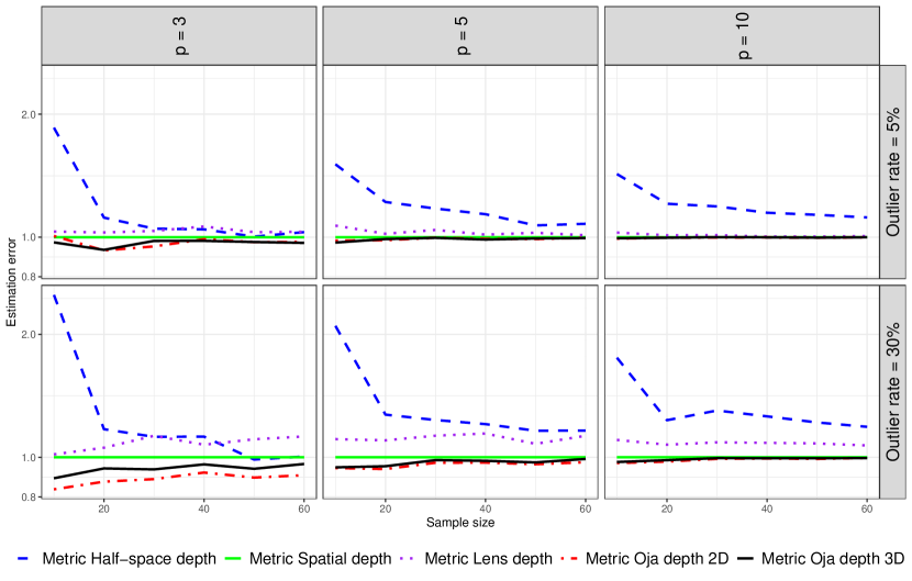
Figure 8: The average estimation errors for each of the five metric depth functions in the correlation matrix simulation relative to the corresponding error of MSD. The scale of the $y$-axis is logarithmic.

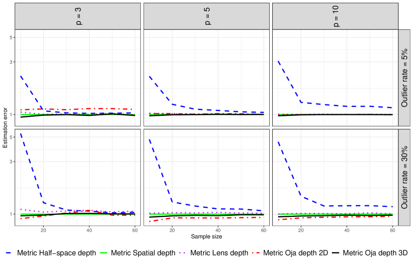
Figure 9: The average estimation errors for each of the five metric depth functions in the hypersphere simulation relative to the corresponding error of MSD. The scale of the $y$-axis is logarithmic.

References

- Barnett [1976] Barnett, V., 1976. The Ordering of Multivariate Data. Journal of the Royal Statistical Society, Series A 139, 318–344. With discussion.
- Bhatia [2009] Bhatia, R., 2009. Positive Definite Matrices. Princeton University Press.
- Cholaquidis et al. [2023] Cholaquidis, A., Fraiman, R., Gamboa, F., Moreno, L., 2023. Weighted Lens Depth: Some Applications to Supervised Classification. Canadian Journal of Statistics 51, 652–673.
- Dai and Lopez-Pintado [2023] Dai, X., Lopez-Pintado, S., 2023. Tukey’s Depth for Object Data. Journal of the American Statistical Association 118, 1760–1772.
- Dubey et al. [2024] Dubey, P., Chen, Y., Müller, H.G., 2024. Metric Statistics: Exploration and Inference for Random Objects with Distance Profiles. Annals of Statistics 52, 757–792.
- Dubey and Müller [2022] Dubey, P., Müller, H.G., 2022. Modeling Time-Varying Random Objects and Dynamic Networks. Journal of the American Statistical Association 117, 2252–2267.
- Eddy [1981] Eddy, W.F., 1981. Graphics for the Multivariate Two-Sample Problem: Comment. Journal of the American Statistical Association 76, 287–289.
- Espezua et al. [2014] Espezua, S., Villanueva, E., Maciel, C.D., 2014. Towards an Efficient Genetic Algorithm Optimizer for Sequential Projection Pursuit. Neurocomputing 123, 40–48.
- Febrero-Bande and Oviedo de la Fuente [2012] Febrero-Bande, M., Oviedo de la Fuente, M., 2012. Statistical Computing in Functional Data Analysis: The R Package fda.usc. Journal of Statistical Software 51, 1–28. URL: https://www.jstatsoft.org/v51/i04/.
- Fischer et al. [2020] Fischer, D., Mosler, K., Möttönen, J., Nordhausen, K., Pokotylo, O., Vogel, D., 2020. Computing the Oja Median in R: The Package OjaNP. Journal of Statistical Software 92, 1–36.
- Fréchet [1948] Fréchet, M., 1948. Les éléments aléatoires de nature quelconque dans un espace distancié. Annales de l’Institut Henri Poincaré 10, 215–310.
- Geenens et al. [2023] Geenens, G., Nieto-Reyes, A., Francisci, G., 2023. Statistical Depth in Abstract Metric Spaces. Statistics and Computing 33, 46.
- Katoch et al. [2021] Katoch, S., Chauhan, S.S., Kumar, V., 2021. A Review on Genetic Algorithm: Past, Present, and Future. Multimedia Tools and Applications 80, 8091–8126.
- Koshevoy and Mosler [1997] Koshevoy, G., Mosler, K., 1997. Zonoid Trimming for Multivariate Distributions. Annals of Statistics 25, 1998–2017.
- Liu [1990] Liu, R.Y., 1990. On a Notion of Data Depth Based on Random Simplices. Annals of Statistics 18, 405–414.
- Liu [1992] Liu, R.Y., 1992. Data Depth and Multivariate Rank Tests, in: Dodge, Y. (Ed.), L1-Statistics Analysis and Related Methods. North-Holland, Amsterdam, pp. 279–294.
- Liu and Modarres [2011] Liu, Z., Modarres, R., 2011. Lens Data Depth and Median. Journal of Nonparametric Statistics 23, 1063–1077.
- Mahalanobis [1936] Mahalanobis, P.C., 1936. On the Generalized Distance in Statistics. Proceedings of the National Institute of Science (India) 2, 49–55.
- Maronna et al. [2019] Maronna, R.A., Martin, R.D., Yohai, V.J., Salibián-Barrera, M., 2019. Robust Statistics: Theory and Methods (with R). John Wiley & Sons.
- Mosler and Mozharovskyi [2022] Mosler, K., Mozharovskyi, P., 2022. Choosing Among Notions of Multivariate Depth Statistics. Statistical Science 37, 348–368.
- Niinimaa and Oja [1995] Niinimaa, A., Oja, H., 1995. On the Influence Functions of Certain Bivariate Medians. Journal of the Royal Statistical Society: Series B (Methodological) 57, 565–574.
- Nordhausen et al. [2022] Nordhausen, K., Oja, H., Tyler, D.E., Virta, J., 2022. ICtest: Estimating and Testing the Number of Interesting Components in Linear Dimension Reduction. URL: https://CRAN.R-project.org/package=ICtest. r package version 0.3-5.
- Oja [1983] Oja, H., 1983. Descriptive Statistics for Multivariate Distributions. Statistics & Probability Letters 1, 327–332.
- Pawlowsky-Glahn and Buccianti [2011] Pawlowsky-Glahn, V., Buccianti, A., 2011. Compositional Data Analysis. Wiley Online Library.
- Ramsay [2024] Ramsay, J., 2024. FDA: Functional Data Analysis. URL: https://CRAN.R-project.org/package=fda. R package version 6.1.8.
- Ramsay and Silverman [2005] Ramsay, J., Silverman, B., 2005. Functional Data Analysis. Springer.
- Scrucca [2013] Scrucca, L., 2013. GA: A package for genetic algorithms in R. Journal of Statistical Software 53, 1–37.
- Scrucca [2017] Scrucca, L., 2017. On Some Extensions to GA Package: Hybrid Optimisation, Parallelisation and Islands Evolution. R Journal 9.
- Serfling [2002] Serfling, R., 2002. A Depth Function and a Scale Curve Based on Spatial Quantiles, in: Dodge, Y. (Ed.), Statistical Data Analysis Based on the L1-Norm and Related Methods. Birkhäuser, Basel. Statistics for Industry and Technology, pp. 25–38.
- Simeon et al. [2022] Simeon, G., Piella, G., Camara, O., Pareto, D., 2022. Riemannian Geometry of Functional Connectivity Matrices for Multi-Site Attention-Deficit/Hyperactivity Disorder Data Harmonization. Frontiers in Neuroinformatics 16, 769274.
- Stewart [1980] Stewart, G.W., 1980. The Efficient Generation of Random Orthogonal Matrices with an Application to Condition Estimators. SIAM Journal on Numerical Analysis 17, 403–409. doi:10.1137/0717034.
- Tukey [1975] Tukey, J.W., 1975. Mathematics and the Picturing of Data, in: James, R. (Ed.), Proceedings of the International Congress of Mathematicians, Canadian Mathematical Congress. pp. 523–531.
- Vardi and Zhang [2000] Vardi, Y., Zhang, C.H., 2000. The Multivariate -median and Associated Data Depth. Proceedings of the National Academy of Sciences 97, 1423–1426.
- Virta [2023a] Virta, J., 2023a. Measure of Shape for Object Data. arXiv preprint arXiv:2312.11378 .
- Virta [2023b] Virta, J., 2023b. Spatial Depth for Data in Metric Spaces. arXiv preprint arXiv:2306.09740 .
- Virta et al. [2022] Virta, J., Lee, K.Y., Li, L., 2022. Sliced Inverse Regression in Metric Spaces. Statistica Sinica 32, 2315–2337.
- Yang and Modarres [2018] Yang, M., Modarres, R., 2018. -skeleton Depth Functions and Medians. Communications in Statistics - Theory and Methods 47, 5127–5143.
- Zhang et al. [2023] Zhang, Q., Xue, L., Li, B., 2023. Dimension Reduction for Fréchet Regression. Journal of the American Statistical Association , 1–15.
- Zhu and Müller [2023] Zhu, C., Müller, H.G., 2023. Geodesic Optimal Transport Regression. arXiv preprint arXiv:2312.15376 .
- Zuo and Serfling [2000] Zuo, Y., Serfling, R., 2000. General Notions of Statistical Depth Function. Annals of Statistics 28, 461–482.