Abstract

We report the result of the numerical lattice computation of the lepton anomalous magnetic moment in QED up to five loops. We concentrate on the contributions from diagrams without lepton loops, which are the most difficult part of the calculation in the Feynman diagram method while the lattice formulation is the easiest. Good agreement with the results of the Feynman diagram method is observed.

1 Introduction

The anomalous magnetic moment of the electron and the muon, $(g-2)_{e/\mu}$, are the most well measured and most precisely calculated quantities in particle physics. The comparison between the theory calculations and the experimental measurements has given us the precision test of the quantum field theory at the level of $10^{-10}$. The largest contribution to $g-2$ is that from QED, where the coefficients of the perturbative expansion in terms of $\alpha\simeq 1/137$ are calculated up to the order of $\alpha^{5}$, corresponding to the Feynman diagrams which contain five loops. There are more than 10,000 diagrams at the five-loop order, and the estimation of the size of those contributions has been necessary for the comparison between the theory and experiments. (For reviews, see Refs. [1, 2].)

Two independent groups have achieved the complete calculation of the five-loop coefficients numerically [3, 4]. The most difficult part of the calculation is the contributions from the diagrams without lepton loops as such diagrams give the most severe infrared (IR) divergences. There are about 6,000 diagrams of such type and somehow give the dominant part of the total contributions. Until recently, there have been a discrepancy in the no-lepton-loop part of the calculation between two groups. The resolution of the discrepancy has been reported in a recent workshop [5].

In this paper, we report the results of the independent method of the calculation based on the lattice QED simulation. The method to evaluate $g-2$ on the lattice has been proposed and developed in Refs. [6, 7]. In particular, the no-lepton-loop part of the calculation corresponds to ignoring the fermion determinant in the path integral. In QED, ignoring the fermion determinant leads to the free theory of the gauge field, $A_{\mu}$, and thus the path integral can be trivially performed by generating gaussian noises. Also, the absence of the lepton loop means that there is no renormalization of $\alpha$, and thus the perturbative expansion can simply be formulated as those in terms of the bare parameter in the Dirac operator. Although the difficulty caused by the severe infrared divergences may be common, the lattice formulation of the calculation is significantly simplified by concentrating on that part.

With the understanding of the possible uncertainties of the method studied in Ref. [7], we performed simulations with large lattice volumes on supercomputers. We evaluated the perturbative coefficients up to five loops, and obtained consistent results with those of two groups.

2 Lattice formulation of quenched QED

Since we concentrate on the Feynman diagrams without lepton loops, one can ignore the fermion action in generating the configurations of the photon field. As it is usual in the lattice simulation, the correlation functions are obtained as the statistical averages of quantities evaluated under each configurations.

The QED without the fermion action is a free theory. The Euclidean lattice action in the Feynman gauge can be written as

$$S_{\rm QED}={1\over 2}\sum_{n,\mu}\hat{A}_{\mu}(n)(-\nabla^{2}+m_{\gamma}^{2})\hat{A}_{\mu}(n).$$ (1)

Here we take the unit of $a=1$ with $a$ the lattice spacing. We recover $a$ in the following discussion when it is necessary. The photon field, $\hat{A}_{\mu}(n)$, is a ultraviolet (UV) regularized one defined by acting a differential operator,

$$\hat{A}_{\mu}(n)\equiv H\left(-{\nabla^{2}\over\Lambda_{\rm UV}^{2}}\right)A_{\mu}(n),$$ (2)

with a function $H(x)$ to satisfy $H(x)\to 0$ for $x\gg 1$ and $H(x)\to 1$ for $x\ll 1$. In this study, we take a sharp UV cut-off,

$$H(x)=\left\{\begin{array}[]{ll}0,&x\geq 1,\\ 1,&x<1.\end{array}\right.$$ (5)

In QED, this simple cut-off is gauge invariant. In the momentum space, the action is diagonalized, and the path integral is a product of gaussian integrals for each momentum modes. For momentum modes with $k^{2}\geq\Lambda_{\rm UV}^{2}$, the UV regulator eliminates their fluctuations while lower modes untouched. The IR divergence for the $k^{2}=0$ mode is regularized by the finite photon mass, $m_{\gamma}$. By this simple set-up, one can generate the photon configurations trivially by generating gaussian noises for each momentum modes up to $k^{2}<\Lambda_{\rm UV}^{2}$ with the variance of $1/(k^{2}+m_{\gamma}^{2})$ and then performing Fourier transform to get back to the position space. The UV cut-off is not formally necessary as the finite lattice spacing in a finite box already replaces the momentum integral to a finite summation. Nevertheless, the introduction of $\Lambda_{\rm UV}$ is numerically necessary in order to suppresses large logarithmic factors which make the continuum limit further [6].

For the calculations of the correlation functions, we use the naive Dirac operator on the lattice:

$$(D)_{nm}^{\alpha\beta}=m\delta_{nm}\delta_{\alpha\beta}+{1\over 2}\sum_{\mu}\left[(\gamma_{\mu})_{\alpha\beta}e^{ieA_{\mu}(n)}\delta_{n+\mu,m}-(\gamma_{\mu})_{\alpha\beta}e^{-ieA_{\mu}(n-\mu)}\delta_{n-\mu,m}\right].$$ (6)

There are unwanted doublers in the propagators obtained by inverting this Dirac operator. We will take care of those unwanted modes later. The parameter $m$ is the fermion mass and $e$ is the coupling constant. We formally expand every quantities in terms of $e$, and evaluate the statistical averages of each coefficients. In this way, at any stage of the calculation, we do not need a specific value of $e$. The coupling constant $e$ is not a parameter in the simulation. This part is different from lattice simulations of non-perturbative dynamics where the continuum limit is taken by tuning the coupling constant to a critical value.

Since there is no lepton loop in our study, $e$ will not be renormalized. This means that $e$ can be identified as the physical coupling constant, i.e., $\alpha=e^{2}/(4\pi)\simeq 1/137$, otherwise, we would need to re-expand $e$ by physical $\alpha$. The perturbative coefficients we evaluate are going to be the physical quantities after taking various limits discussed below and can be compared with the ones from the Feynman diagram calculations.

The limits we should take are $\Lambda_{\rm UV}\to\infty$, $m_{\gamma}\to 0$, and $a\to 0$ while fixing the fermion mass $m$ to be finite to bring back to the continuum QED. In practice, we fix $\Lambda_{\rm UV}a=1.5$, and take the limit of $m_{\gamma}/m\to 0$ and $ma\to 0$. We also need to take $L\to\infty$ and $T\to\infty$, where $L$ and $T$ are the lattice sizes in the spacial and the temporal directions, respectively. Since we introduce the photon mass $m_{\gamma}$ as the IR regulator, the finite volume effects are suppressed exponentially as $e^{-m_{\gamma}L}$ and $e^{-m_{\gamma}T}$. Therefore, we keep the combinations of $m_{\gamma}L$ and $m_{\gamma}T$ large enough in the calculation so that we do not have to deal with $O(1/L)$ or $O(1/T)$ corrections.

3 $g$-factor measurements on the lattice

We measure fermion-fermion-current three point functions to obtain the form factors. We work in the position space in the Euclidean temporal direction and in the momentum space in the spacial direction.

We evaluate the three-point function as follows. Under each photon configuration, $A_{\mu}(n)$, which is generated according to the free field theory, we evaluate the quantity inside the bracket of

$$G_{\mu}(t)=\Big{\langle}\sum_{\bf p^{\prime}}D^{-1}(t_{\rm sink},t;{\bf p},{\bf p}^{\prime})\gamma_{\mu}D^{-1}(t,t_{\rm src};{\bf p^{\prime}+k},{\bf p+k})\Big{\rangle},$$ (7)

and take the ensemble average, $\langle\cdots\rangle$. The locations $t_{\rm src}$, $t_{\rm sink}$ and $t$ are those of two fermions and the current operator, respectively. We fix $t_{\rm src}$ and $t_{\rm sink}$ at some particular locations, and view the correlation function as a function of $t$ for later purpose. The momenta ${\bf p}$ and ${\bf k}$ are those of the outgoing fermion and the photon (the current vertex). We take ${\bf k}$ to be the smallest non-zero momentum on the lattice, ${\bf k}=(0,0,2\pi/L)$, and ${\bf p}=-{\bf k}/2$ so that the incoming and the outgoing fermion momenta, ${\bf p+k}$ and ${\bf p}$, are in the back-to-back configuration. The half-integer momentum of the fermions can be realized by taking the anti-periodic boundary condition in the $z$ direction. For the $g$ factor calculation, we need to take the limit of ${\bf p}={\bf k}=0$. This causes an error of $O(1/L^{2})$ that we ignore. The inverse of the Dirac operator represents the propagation of the fermion under the photon background. In the calculation of the no-lepton-loop diagrams, one can ignore the disconnected diagram which directly connects $t_{\rm src}$ to $t_{\rm sink}$ and $t$ to $t$, since the latter propagator forms a fermion loop. All the Feynman diagrams are, therefore, included in Eq. (7). In the definition of the three-point function, we use the naive current operator $\bar{\psi}\gamma_{\mu}\psi$, which is non-conserving on the lattice. The renormalization of the vertex will be discussed later.

The inversion of the Dirac operator, $D$, can be taken perturbatively by the use of the Fourier transform [8]. This is basically the same procedure as the Feynman diagram calculation. The full propagator of the fermion at each order in the perturbative expansion is given by the product of the free propagators and the vertices. The vertices are associated with the photon field $A_{\mu}(n)$ that is a function in the position space. The free fermion propagator is a diagonal matrix (a function of a single momentum $k_{\mu}$) in the momentum space. The multiplication of functions, i.e., diagonal matrices, can be done quickly on computers, and the Fourier transform between the position and momentum spaces can also be effectively performed by the use of the fast Fourier transform (FFT) algorithm. In this way, the multiple-dimensional integrations of loop momenta in the Feynman diagram calculation are numerically encoded as a series of FFTs and all the different Feynman diagrams are summarized as a single term in Eq. (7).

For large enough separations of $t_{\rm sink}$, $t_{\rm src}$, and $t$, the three-point function is dominated by contributions from the lowest energy state, that is the on-shell fermion. One can extract the physical form factors of the fermion by taking such a set-up. One complication is that there are also contributions from the doubler state in the time direction. The doubler contribution gives alternative signs for even and odd values of $t_{\rm sink}-t_{\rm src}$ because the on-shell pole is at $E=m_{*}+i\pi$ and the propagator is proportional to $e^{-Et}$. One can therefore remove them by taking an average with the next site. For the choice of our external momentum, ${\bf p}=-({\bf p+k})$, an easier treatment is possible thanks to the parity symmetry of the fermion configuration. The doubler contributions to the form factors are identical to the physical ones for odd separations of $t_{\rm sink}-t_{\rm src}$, whereas it completely cancels out the physical ones for even separations. Therefore, one can remove the doubler contributions by setting an odd separation of $t_{\rm sink}-t_{\rm src}$ and taking an appropriate normalization as we see later. For spacial directions, there is no doubler contribution since we work in the momentum space.

Here we define projections to the electric and the magnetic functions:

$$G_{E}(t)={\rm tr}\left[{1+\gamma_{4}\over 2}G_{4}(t)\right],\quad G_{M}(t)=i\sum_{i,j,k}\epsilon_{ijk}{\rm tr}\left[{1+\gamma_{4}\over 2}\gamma_{5}\gamma_{i}G_{j}(t)\right]{\bf k}_{k},$$ (8)

where $i,j,k$ are indices for the spacial directions, $x$, $y$ and $z$. The Euclidean temporal direction is labelled as 4. The trace is taken over the spinor indices. The Dirac representation of the gamma matrices is convenient here since the projection, $(1+\gamma_{4})/2$, simply picks up the upper two components of the source and sink spinors. One can take away the external fermion legs and obtain the form factors by

$$F_{E}(t)={G_{E}(t)\over G_{E}^{\rm norm}(t)},\quad F_{M}(t)={G_{M}(t)\over G_{M}^{\rm norm}(t)},$$ (9)

where $G_{E}^{\rm norm}(t)$ and $G_{M}^{\rm norm}(t)$ are calculated from the combination of the two-point functions:

$$G_{\mu}^{\rm norm}(t)=\sum_{\bf p^{\prime}}\Big{\langle}D^{-1}(t_{\rm sink},t;{\bf p},{\bf p}^{\prime})\Big{\rangle}\gamma_{\mu}\Big{\langle}D^{-1}(t,t_{\rm src};{\bf p^{\prime}+k},{\bf p+k})\Big{\rangle}.$$ (10)

The doubler contribution is cancelled as both numerators and denominators are multiplied by two. The $g$ factor can now be obtained as the ratio of the electric and the magnetic form factors:

$${g(t)\over 2}={F_{M}(t)\over F_{E}(t)},$$ (11)

up to a correction from finite ${\bf k}$. For large enough separations of $t$ from $t_{\rm src}$ and $t_{\rm sink}$, $g(t)$ should be independent of $t$. By looking for a plateau as a function of $t$, one can obtain the $g$ factor numerically. Again, all the quantities are expanded in terms of the power series of $e$ at any stage of calculation. Namely, the multiplication and the inversion are encoded as the rules for each perturbative coefficients in the computer program. Therefore, at the end of the calculation, we obtain numerical evaluation of the coefficients.

The renormalization is implicitly done in this flow of calculation. For taking away the fermion legs, we use the full propagator in Eq. (10). This can be thought of as the wave function and the mass renormalizations. In Eq. (11), we take the ratio of the electric and the magnetic form factors. This is nothing but the vertex renormalization to normalize $F_{E}$ to unity.

The method described here is slightly different from the previous works in Refs. [6, 7], where the correlation functions are calculated in the momentum space and the double pole part associated with two fermion propagators are extracted by the Fourier transform and extrapolation. Two methods give the same form factors in the continuum limit, but we take the position space calculation here since it is more transparent.

4 Numerical results

We perform the lattice simulations with five sets of lattice volumes, $L^{3}\times T$ = $24^{3}\times 48$, $28^{3}\times 56$, $32^{3}\times 64$, $48^{3}\times 96$, and $64^{3}\times 128$, where simulations are performed on NEC SX-Aurora TSUBASA A500-64 at KEK for smaller four volumes up to $48^{3}\times 96$, and on supercomputer Fugaku at RIKEN for $64^{3}\times 128$. We also performed a simulation with the $96^{3}\times 192$ lattice volume on Fugaku with small statistics as a trial. For the Fugaku platform, we developed a computer code to make high parallelization possible based on the public lattice simulation code Bridge++ [9].

For each lattice volume, we fix the fermion mass parameter to be $ma=2.04/\sqrt{L}$, and take five points of the photon mass parameter, $m_{\gamma}a=4/L$, $5/L$, $6/L$, $7/L$, and $8/L$. (We take only $m_{\gamma}a=4/L$ for $L=96$.) The UV cut-off is fixed as $\Lambda_{\rm UV}a=1.5$ for all the volumes. The source location is fixed as $t_{\rm src}=0$ and $t_{\rm sink}$ is taken to be the largest odd integer below $3T/4$. We take the average of the periodic and anti-periodic boundary conditions in the temporal direction in evaluating the inverse of the Dirac operators [7]. This treatment effectively doubles the time extent $T$. The contribution from the backward propagation on the torus to connect $t_{\rm src}$ and $t_{\rm sink}-T\sim t_{\rm sink}$ is cancelled even though it is actually closer for our choice of $t_{\rm src}$ and $t_{\rm sink}$.

The finite volume effects are controlled by the $e^{-m_{\gamma}L}$ factor, that is at most a few percent for each parameter points. Barring this level of errors, one can interpret all the data to be equivalent to the ones obtained with infinite volume with finite $m_{\gamma}$ and $a$. For larger $L$ simulations, one can take smaller values of $m_{\gamma}/m$ as well as smaller $ma$. As explained before, we need to take two limits $ma\to 0$ and $m_{\gamma}/m\to 0$ while $\Lambda_{\rm UV}a$ fixed to reach to the continuum QED.

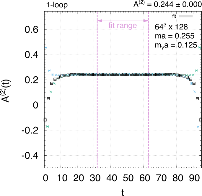
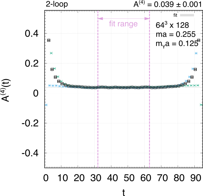
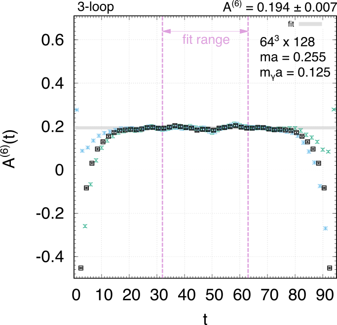
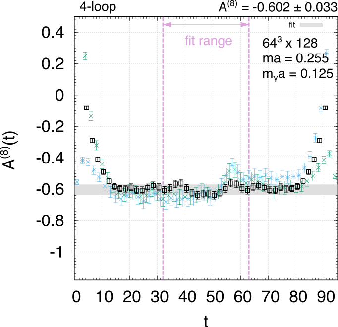
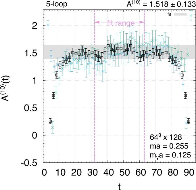
Figure 1: The perturbative coefficients of $g(t)/2$ defined in Eq. (11) and (12) for the $64^{3}\times 128$ lattice with $m_{\gamma}a=0.125$ and $ma=0.255$. The left and right end of $t$ is the source and the sink location, and $t$ is the location of the current operator.

We show in Fig. 1 the perturbative coefficients $A^{(2n)}(t)$ of the $g(t)$ function in Eq. (11) defined as

$${g(t)\over 2}=1+A^{(2)}(t)\left({\alpha\over\pi}\right)+A^{(4)}(t)\left({\alpha\over\pi}\right)^{2}+\cdots.$$ (12)

We show data for the $64^{3}\times 128$ lattice with $m_{\gamma}a=8/L=0.125$. We analyzed about 200,000 configurations for this parameter set. One can observe plateaus in the middle region of $t$. The data for even (green $\times\hbox to0.0pt{\hss+}$) and odd $t$ (blue $\times$) behave differently due to the contributions from doublers associated with the higher excited modes. The average between next two points are shown as black squares. We take the average of the middle region ($T/4\leq t<T/2$) as the value of the plateau, and define the average as $A^{(2n)}$ at the $n$-loop order.

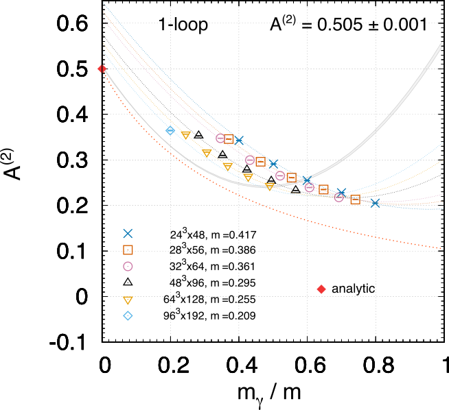
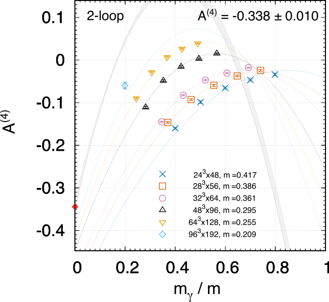
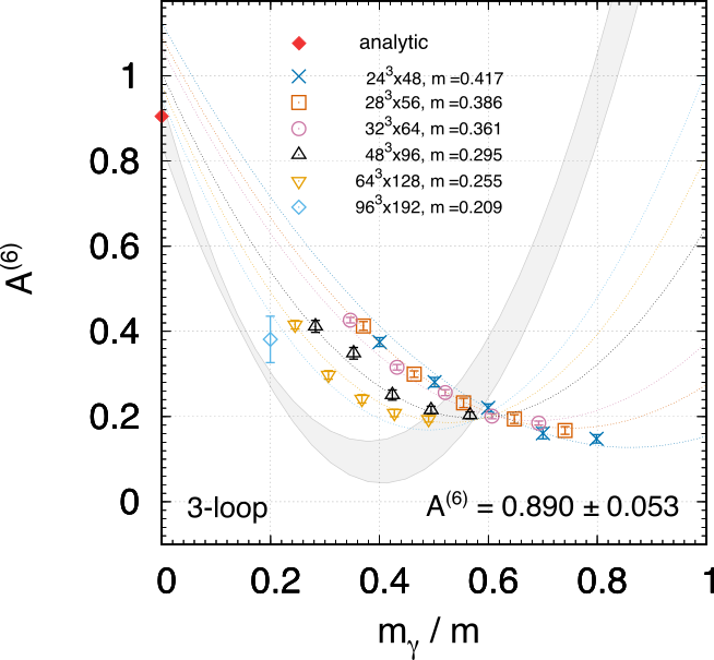
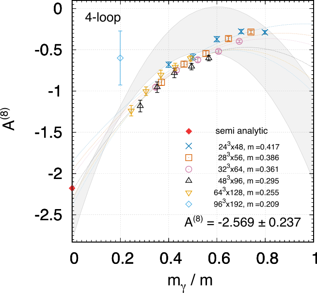
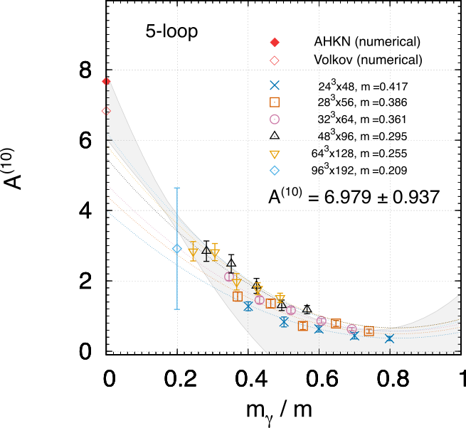
Figure 2: The coefficients of the perturbative expansion of $g/2$ at finite $m_{\gamma}a$ and $ma$. By the fitting with Eq. (13), we obtain the continuum limit as the gray band. The red diamonds represent the known results by the Feynman diagram method to be compared with the section of the gray band at $m_{\gamma}/m=0$. The red dotted curve at the one-loop level is the analytic results in the continuum theory.

The values of $A^{(2n)}$ for each parameter set are shown as a function of $m_{\gamma}/m$ in Fig. 2. We perform fitting of those points by the following function to extrapolate to $ma\to 0$ and $m_{\gamma}/m\to 0$:

$$A^{(2n)}(m,m_{\gamma})= a_{0}^{(2n)}\left(1+b_{0}^{(2n)}(ma)^{2}\right)$$

$$+a_{1}^{(2n)}{m_{\gamma}\over m}\left(1+b_{1}^{(2n)}(ma)\right)+a_{2}^{(2n)}\left({m_{\gamma}\over m}\right)^{2}\left(1+b_{2}^{(2n)}(ma)\right),$$ (13)

with $a_{0-2}^{(2n)}$ and $b_{0-2}^{(2n)}$ as parameters for each $n$-loop order. The results of the fitting to the continuum limit, $ma\to 0$, are shown as gray bands (1$\sigma$) in each figure. We take into account up to the quadratic order in $m_{\gamma}/m$, and the leading correction in terms of $ma$ is included. The leading correction at the zero-th order of $m_{\gamma}/m$ is $O((ma)^{2})$ due to chiral symmetry. Since we maintain chiral symmetry on the lattice by using the naive Dirac operator, there is no $O(ma)$ correction towards the continuum limit. For higher orders in $m_{\gamma}/m$, there can be $O(m_{\gamma}a)$ or $O(m_{\gamma}^{2}a/m)$ corrections, that we take into account in the fitting. As one can see from the figures, the $m_{\gamma}/m\to 0$ limit is quite far from the data points we obtained. We cannot, however, take arbitrarily small $m_{\gamma}/m$ as we need to keep the combination of $m_{\gamma}L$ to be large enough to suppress the finite volume corrections while $ma$ needs to be close enough to the continuum limit, $ma\to 0$. This difficulty can be understood as reflection of severe IR divergences in this set of diagrams.

At one-loop, the red dotted curve is the analytic calculation of $A^{(2)}$ as a function of the finite photon mass in the continuum theory. Even though it is a quite large extrapolation, we find a good agreement at the small $m_{\gamma}/m$ region. The fitting results at $m_{\gamma}/m=0$ at each order should be compared with the red diamonds which represent the known results from the diagrammatic calculations. (We take the values up to four loops from the table in Ref. [10]. For five loops, see below for explanation.) The fitting results at each order are shown in the figures. We see quite good agreements. The results seem to be indicating that the systematic uncertainties, such as the finite volume effects and the one associated with the fitting function are under good control.

Our estimation of the five-loop coefficients, $A^{(10)}$, is

$$A^{(10)}({\mbox{no lepton loop}})=7.0\pm 0.9,$$ (14)

where only the statistical error is taken into account. The value is consistent with the result of Ref. [4] ($6.828\pm 0.060$, open diamond). There was a tension between this value and the AHKN result ($7.668\pm 0.159$, filled diamond) in Refs. [3, 1]. It has been reported recently that a new preliminary AHKN result is now consistent with Ref. [4] within 1$\sigma$ [5]. In any case, our result seems to be giving a good estimate of the five-loop coefficient.

5 Summary

We continued the trial to obtain the perturbative coefficients of $g-2$ in QED by using lattice simulations. The calculation is quite simple as we only have a single diagram to evaluate. By concentrating on the diagrams without a lepton loop, the formulation is further simplified as one can generate photon configurations by the free theory. We obtain results which are consistent with the Feynman diagram method. Further improvement of the statistical precision seems to be possible. The data points of the largest lattice, $96^{3}\times 192$, are obtained with a trial run with about 20,000 configurations. Ten times large statistics with several different values of $m_{\gamma}$ should easily be possible if computational time is allocated.

Although one probably needs to be more careful about the possible systematic errors to give more reliable predictions, our calculation here is meant to be the confirmation of the previous calculations by estimating the size of the perturbative coefficients by a totally independent method. If we need to estimate the coefficient at the six-loop order by future progress in experimental precisions (which is indeed expected [12]), the method presented here may serve as the first thing to try as the computational cost scales only as $(2n)^{2}$ with $n$ the loop order while the number of Feynman diagrams grows as more than $(2n)!$ [13, 14].

Including the with-lepton-loop part is possible along the line of the method in Ref. [6]. In this case, we need to generate configurations according to the Langevin equations [8] where the inversion of the Dirac operator is needed in each Langevin step. Although the formulation is more complicated, the cost of the computation may not be so heavy since less severe IR divergence may mean that we need less statistics.

References

- [1] T. Aoyama, T. Kinoshita, and M. Nio, “Theory of the Anomalous Magnetic Moment of the Electron,” Atoms 7 no. 1, (2019) 28.
- [2] T. Aoyama et al., “The anomalous magnetic moment of the muon in the Standard Model,” Phys. Rept. 887 (2020) 1–166, arXiv:2006.04822 [hep-ph].
- [3] T. Aoyama, M. Hayakawa, T. Kinoshita, and M. Nio, “Complete Tenth-Order QED Contribution to the Muon g-2,” Phys. Rev. Lett. 109 (2012) 111808, arXiv:1205.5370 [hep-ph].
- [4] S. Volkov, “Calculation of the total 10th order QED contribution to the electron magnetic moment,” Phys. Rev. D 110 no. 3, (2024) 036001, arXiv:2404.00649 [hep-ph].
- [5] “Seventh plenary workshop of the muon theory initiative,” KEK Tsukuba campus, Japan, September 9-13, 2024. https://conference-indico.kek.jp/event/257/.
- [6] R. Kitano, H. Takaura, and S. Hashimoto, “Stochastic computation of in QED,” JHEP 05 (2021) 199, arXiv:2103.10106 [hep-lat].
- [7] R. Kitano and H. Takaura, “Quantum electrodynamics on the lattice and numerical perturbative computation of ,” PTEP 2023 no. 10, (2023) 103B02, arXiv:2210.05569 [hep-lat].
- [8] F. Di Renzo and L. Scorzato, “Fermionic loops in numerical stochastic perturbation theory,” Nucl. Phys. B Proc. Suppl. 94 (2001) 567–570, arXiv:hep-lat/0010064.
- [9] S. Ueda, S. Aoki, T. Aoyama, K. Kanaya, H. Matsufuru, S. Motoki, Y. Namekawa, H. Nemura, Y. Taniguchi, and N. Ukita, “Development of an object oriented lattice QCD code ’Bridge++’,” J. Phys. Conf. Ser. 523 (2014) 012046.
- [10] S. Volkov, “New method of computing the contributions of graphs without lepton loops to the electron anomalous magnetic moment in QED,” Phys. Rev. D 96 no. 9, (2017) 096018, arXiv:1705.05800 [hep-ph].
- [11] T. Aoyama, T. Kinoshita, and M. Nio, “Revised and Improved Value of the QED Tenth-Order Electron Anomalous Magnetic Moment,” Phys. Rev. D 97 no. 3, (2018) 036001, arXiv:1712.06060 [hep-ph].
- [12] X. Fan, T. G. Myers, B. A. D. Sukra, and G. Gabrielse, “Measurement of the Electron Magnetic Moment,” Phys. Rev. Lett. 130 no. 7, (2023) 071801, arXiv:2209.13084 [physics.atom-ph].
- [13] R. J. Riddell, “The number of feynman diagrams,” Phys. Rev. 91 (Sep, 1953) 1243–1248. https://link.aps.org/doi/10.1103/PhysRev.91.1243.
- [14] P. Cvitanovic, B. E. Lautrup, and R. B. Pearson, “The Number and Weights of Feynman Diagrams,” Phys. Rev. D 18 (1978) 1939.