\shortdate
\msc

49K40, 93D23, 47D03, 35G31

Stability and decay rate estimates for a nonlinear dispersed flow reactor model with boundary control

Yevgeniia Yevgenieva Max Planck Institute for Dynamics of Complex Technical Systems, 39106 Magdeburg, Germany

Institute of Applied Mathematics and Mechanics, National Academy of Sciences of Ukraine,
84116 Sloviansk, Ukraine
, \orcid0000-0002-1867-3698
yevgenieva@mpi-magdeburg.mpg.de
Alexander Zuyev Max Planck Institute for Dynamics of Complex Technical Systems, 39106 Magdeburg, Germany

Institute of Applied Mathematics and Mechanics, National Academy of Sciences of Ukraine,
84116 Sloviansk, Ukraine
, \orcid0000-0002-7610-5621
zuyev@mpi-magdeburg.mpg.de
  Peter Benner Max Planck Institute for Dynamics of Complex Technical Systems, 39106 Magdeburg, Germany
, \orcid0000-0003-3362-4103
benner@mpi-magdeburg.mpg.de
Abstract

We investigate a nonlinear parabolic partial differential equation whose boundary conditions contain a single control input. This model describes a chemical reaction of the type “$A\to$ product”, occurring in a dispersed flow tubular reactor. The existence and uniqueness of solutions to the nonlinear Cauchy problem under consideration are established by applying the theory of strongly continuous semigroups of operators. Using Lyapunov’s direct method, a feedback control design that ensures the exponential stability of the steady state is proposed, and the exponential decay rate of solutions is evaluated.

keywords:
chemical reaction model, boundary control, nonlinear parabolic partial differential equations, existence and uniqueness of solutions, exponential stability, decay rate of solutions, feedback control design
\novelty

The key contribution of our work is the following:

  • A class of feedback controllers is designed to achieve exponential stability of the steady-state solution in the closed-loop system.

  • The existence and uniqueness of solutions of the model with the proposed controllers are proved.

  • An evaluation of the solution’s decay rate is presented.

  • Numerical simulations are presented to illustrate the large-time behavior of solutions to the closed-loop system under consideration.

1 Introduction

In recent years, there has been significant research into chemical reaction models, particularly in the context of boundary control, which provides a natural means of regulating the process. In tubular reactors, boundary control focuses on manipulating inlet concentrations, temperatures, and flow rates to adjust the reaction rate and maintain the desired process performance.

The development of control strategies for optimizing and stabilizing chemical reactions is crucial in chemical engineering. Various papers [1, 7, 11, 12] have explored optimal control strategies aimed at maximizing product yield while utilizing a fixed amount of reactants.

Stabilization is essential for ensuring consistent and reliable operation under varying conditions, leading to improved process efficiency, product quality, and safety. In chemical reactions, exponential stability refers to the system’s ability to rapidly converge to a stable operating state following perturbations or disturbances.

The exponential stabilization of several classes of linear and nonlinear parabolic equations with boundary control has been investigated in numerous papers (see, e.g., [8, 9, 10] and references therein).

In our study, we focus on the mathematical model of a chemical reaction conducted in a dispersed flow tubular reactors (DFTR) and apply an explicit boundary feedback control scheme to characterize the exponential stability property of this model.

2 Basic notations and auxiliary results

This section presents the notations and theorems used throughout the paper.

Basic notations $C^{2}[a,b]$ the set of continuous functions on $[a,b]$ with continuous derivatives up to the second order; $L^{1}(a,b)$ the set of all measurable real functions on $(a,b)$ for which the Lebesgue integral $\int_{a}^{b}f(x)\,dx$ exists and is finite; $L^{2}(a,b)$ the Hilbert space of all measurable real functions on $(a,b)$ whose squared absolute values are Lebesgue integrable; $||f||_{L^{2}(a,b)}$ $:=\left(\int_{a}^{b}|f(x)|^{2}\,dx\right)^{\frac{1}{2}}$, the norm in $L^{2}(a,b)$; $\left<f,g\right>_{L^{2}(a,b)}$ $:=\int_{a}^{b}f(x)g(x)\,dx$, the inner product in $L^{2}(a,b)$; $L^{\infty}(a,b)$ the set of all measurable real functions on $(a,b)$ that are bounded almost everywhere on $(a,b)$; $H^{2}(a,b)$ the Hilbert space of functions in $L^{2}(a,b)$ whose weak derivatives up to the second order also belong to $L^{2}(a,b)$.

Theorem 2.1 (Lumer–Phillips theorem [6]).

Let $\mathcal{A}:D(A)\to X$ be a linear operator defined on a subset $D(\mathcal{A})$ of a Banach space $X$. Then $\mathcal{A}$ generates a strongly continuous semigroup of operators on $X$ if and only if:

  • (i)

    $D(\mathcal{A})$ is dense in $X$;

  • (ii)

    $\mathcal{A}$ is dissipative;

  • (iii)

    $R(\mathcal{A}-\lambda\mathcal{I})=X$ for some $\lambda>0$, where $R$ denotes the range of the operator and $\mathcal{I}$ denotes the identity operator.

Theorem 2.2 ([4, Chapter 2, Proposition 5.3]).

Let the linear operator $\mathcal{A}:D(\mathcal{A})\to X$ generate a $C_{0}$ semigroup $\{e^{t\mathcal{A}}\}_{t\geqslant 0}$ and let $f:X\to X$ be the operator satisfying the following:

$\displaystyle\|f(x_{1})-f(x_{2})\|_{X}$ $\displaystyle\leqslant\mu(t)\|x_{1}-x_{2}\|_{X},\quad\forall\,t\in[0,T],\ \forall\,x_{1},x_{2}\in X,$ (2.1)
$\displaystyle\|f(0)\|_{X}$ $\displaystyle\leqslant\mu(t),\quad\forall\,t\in[0,T],$

with some function $\mu\in L^{1}(0,T)$. Then, the equation

$$y(t)=e^{t\mathcal{A}}y_{0}+\int_{0}^{t}e^{(t-s)\mathcal{A}}f(y(s))ds,\quad t\in[0,T]$$

admits a unique solution $y$ for any $y_{0}\in X$.

3 Description of the model

Consider the mathematical model of a DFTR represented by the nonlinear parabolic equation with the following Danckwerts boundary conditions [5, 7]:

$\displaystyle\frac{\partial C_{A}}{\partial t}$ $\displaystyle=D_{ax}\frac{\partial^{2}C_{A}}{\partial x^{2}}-v\frac{\partial C_{A}}{\partial x}-kC_{A}^{n},\qquad(x,t)\in(0,l)\times(0,T),$ (3.1)
$\displaystyle C_{A}(0,t)$ $\displaystyle=C_{A_{0}}(t)+\frac{D_{ax}}{v}\frac{\partial C_{A}}{\partial x}\Big{|}_{x=0},\quad\frac{\partial C_{A}}{\partial x}\Big{|}_{x=l}=0,$

where $C_{A}(x,t)\geqslant 0$ is the reactant $A$ concentration inside the reactor at the distance $x$ from the inlet and at time $t$, $l$ is the length of the reactor tube, $C_{A_{0}}(t)$ is the concentration of $A$ in the inlet stream (that also contains another inert component), $n>0$ is the reaction order, $D_{ax}>0$ is the axial dispersion coefficient, $v>0$ is the flow-rate of the reaction stream, and $k>0$ is the reaction rate constant. The function $C_{A_{0}}(t)\geqslant 0$ is treated as the control input.

In order to rewrite the problem in an abstract form, we present the steady-state solution $\overline{C}_{A}\in C^{2}[0,l]$ as a solution to the problem:

$\displaystyle D_{ax}\frac{d^{2}\overline{C}_{A}}{dx^{2}}$ $\displaystyle=v\frac{d\overline{C}_{A}}{dx}+k\overline{C}_{A}^{n},\quad x\in(0,l),$ (3.2)
$\displaystyle\overline{C}_{A}(0)$ $\displaystyle=\overline{u}+\frac{D_{ax}}{v}\frac{d\overline{C}_{A}}{dx}\Big{|}_{x=0},\quad\frac{d\overline{C}_{A}}{dx}\Big{|}_{x=l}=0,$

where $\overline{u}=\text{const}>0$ denotes the steady-state control, selected to ensure that the solution $\overline{C}_{A}(x)$ remains non-negative, i.e., $\overline{C}_{A}(x)\geqslant 0$ for all $x\in[0,l]$.

In the following discussion, we reformulate the problem expressed in (3.1) in terms of deviations by introducing the function $w(x,t)=C_{A}(x,t)-\overline{C}_{A}(x)$:

$\displaystyle\frac{\partial w}{\partial t}$ $\displaystyle=D_{ax}\frac{\partial^{2}w}{\partial x^{2}}-v\frac{\partial w}{\partial x}+k\overline{C}_{A}^{n}-k(w+\overline{C}_{A})^{n},\qquad(x,t)\in(0,l)\times(0,T),$ (3.3)
$\displaystyle w(0,t)$ $\displaystyle=u_{w}(t)+\frac{D_{ax}}{v}\frac{\partial w}{\partial x}\Big{|}_{x=0},\quad\frac{\partial w}{\partial x}\Big{|}_{x=l}=0,$

where $u_{w}(t):=C_{A_{0}}(t)-\overline{u}$.

We will investigate the above problem with a boundary feedback control $u_{w}$ in the form

$$u_{w}(t)=\alpha\,w(0,t),\quad\alpha\in\left[0,\tfrac{1}{2}\right].$$ (3.4)

We note that this parameterized class of controls includes also the case $u_{w}(t)\equiv 0$, which represents the steady-state control $\overline{u}$ for the initial problem (3.1).

As the concentration $C_{A}(x,t)$ is nonnegative and bounded from above by a constant due to physical considerations, the reaction model should also satisfy certain constraints in terms of the deviation $w(x,t)$. For this purpose, we introduce the saturation function of $w$ as follows:

$$\text{Sat}_{M}(w):=\begin{cases}w,\quad&\text{if }|w|\leqslant M,\\ M,\quad&\text{if }w>M,\\ -M,\quad&\text{if }w<-M,\end{cases}$$

where $M<\infty$ is a positive constant.

To study the well-posedness of the considered model, we rewrite system (3.3) in an abstract form. First, we introduce the operator $\mathcal{A}:D(\mathcal{A})\to X$ such that

$$\mathcal{A}:{\xi}\in D(\mathcal{A})\mapsto\mathcal{A}{\xi}=(D_{ax}\xi^{\prime\prime}-v\xi^{\prime})\in X,$$ (3.5)

where $X=L^{2}(0,l)$ and, for any $\alpha\in\left[0,\tfrac{1}{2}\right]$,

$$D(\mathcal{A})=D_{\alpha}(\mathcal{A}):=\left\{\xi\in H^{2}(0,l):(1-\alpha)\xi(0)=\frac{D_{ax}}{v}\xi^{\prime}(0),\ \xi^{\prime}(l)=0\right\}.$$

Consider also the nonlinear operator $r:X\to X$ defined by

$$r({\xi})=k\overline{C}_{A}^{n}-k(\text{Sat}_{M}(\xi)+\overline{C}_{A})^{n}.$$

Now, the problem (3.3) can be rewritten in the abstract form for $\xi(t)=w(\cdot,t)$ as follows:

$\displaystyle\dot{{\xi}}(t)$ $\displaystyle=\mathcal{A}\,{\xi}(t)+r({\xi}(t)),$ (3.6)
$\displaystyle\xi(0)$ $\displaystyle=\xi_{0}\in D(\mathcal{A}).$

4 Main results

4.1 Existence and uniqueness of solution to the problem (3.6)

We use the strongly continuous semigroup theory to prove the existence and uniqueness of the mild solution to the problem (3.6). First, we obtain the semigroup generation property for the linear operator $\mathcal{A}$.

Lemma 4.1.

The operator $\mathcal{A}:D(\mathcal{A})\to X$, defined by the relation (3.5), generates the $C_{0}$–semigroup $\{e^{t\mathcal{A}}\}_{t\geqslant 0}$ of bounded linear operators on $X$.

Proof.

The proof of this lemma boils down to verifying the conditions of Theorem 2.1.

First, we check the condition $(ii)$ and show that the operator $\mathcal{A}$ is dissipative, namely, that $\left<\mathcal{A}\xi,\xi\right>_{L^{2}(0,l)}\leqslant 0$ $\forall\,\xi\in D(\mathcal{A})$:

$\displaystyle\left<\mathcal{A}\xi,\xi\right>_{L^{2}(0,l)}$ $\displaystyle=\int_{0}^{l}(D_{ax}\xi^{\prime\prime}-v\xi^{\prime})\xi\,dx=D_{ax}\xi\xi^{\prime}\big{|}_{0}^{l}-D_{ax}\int_{0}^{l}(\xi^{\prime})^{2}dx-\frac{v}{2}\int_{0}^{l}(\xi^{2})^{\prime}dx$
$\displaystyle=-D_{ax}\xi(0)\xi^{\prime}(0)-D_{ax}\int_{0}^{l}(\xi^{\prime})^{2}dx-\frac{v}{2}\xi^{2}(l)+\frac{v}{2}\xi^{2}(0)$
$\displaystyle=-v\left(\frac{1}{2}-\alpha\right)\xi^{2}(0)-D_{ax}\int_{0}^{l}(\xi^{\prime})^{2}dx-\frac{v}{2}\xi^{2}(l)\leqslant 0$

for all $\xi\in D(\mathcal{A})$.

Now, we prove that $D(\mathcal{A})$ is dense in $L^{2}(0,l)$ (condition $(i)$). First, we introduce the set

$$D^{0}(\mathcal{A}):=\left\{\xi\in H^{2}(0,l):\xi(0)=\xi^{\prime}(0)=\xi^{\prime}(l)=0\right\}$$

and prove that $D^{0}(\mathcal{A})$ is dense in $L^{2}(0,l)$. Then, the obvious embedding $D^{0}(\mathcal{A})\subset D(\mathcal{A})\subset L^{2}(0,l)$ ensures that $D(\mathcal{A})$ is dense in $L^{2}(0,l)$.

The denseness proof is similar to the proof of Corollary 4.23 in [2]. Given $\xi\in L^{2}(0,l)$, we set

$$\bar{\xi}=\begin{cases}\xi(x),\quad&\text{if }x\in(0,l),\\ 0,&\text{if }x\in\mathbb{R}\setminus(0,l),\end{cases}$$

so that $\bar{\xi}\in L^{2}(\mathbb{R})$.

Let $\{K_{n}\}$ be a sequence of intervals such that $K_{n}:=\left(\frac{2}{n},l-\frac{2}{n}\right)$. Let $\{\rho_{n}\}$ be a sequence of mollifiers such that

$$\rho_{n}\in C^{\infty}_{c}(\mathbb{R}),\quad\text{supp}\,\rho_{n}\subset\left(-\frac{1}{n},\frac{1}{n}\right),\quad\int_{\mathbb{R}}\rho_{n}(x)dx=1,\quad\rho_{n}(x)\geqslant 0\ \forall\,x\in\mathbb{R}.$$

Set $g_{n}=\chi_{K_{n}}\bar{\xi}$ and

$$\xi_{n}=\rho_{n}*g_{n}:=\int_{\mathbb{R}}\rho_{n}(x-y)\,g_{n}(y)dy,$$

so that $\text{supp}\,\xi_{n}\subset\left(\frac{1}{n},l-\frac{1}{n}\right)$. It follows that $\xi_{n}\in C^{\infty}_{c}(\mathbb{R})$ and, moreover, $\xi_{n}(0)=\xi^{\prime}_{n}(0)=\xi^{\prime}_{n}(l)=0$, so $\xi_{n}\in D^{0}(\mathcal{A})$.

On the other hand, we have

$$||\xi_{n}-\xi||_{L^{2}(0,l)}=||\xi_{n}-\bar{\xi}||_{L^{2}(\mathbb{R})}\leqslant||(\rho_{n}*g_{n})-(\rho_{n}*\bar{\xi})||_{L^{2}(\mathbb{R})}+||(\rho_{n}*\bar{\xi})-\bar{\xi}||_{L^{2}(\mathbb{R})}.$$

By Young’s convolution equation, we get

$$||(\rho_{n}*g_{n})-(\rho_{n}*\bar{\xi})||_{L^{2}(\mathbb{R})}\leqslant||\rho_{n}||_{L^{1}(\mathbb{R})}||g_{n}-\bar{\xi}||_{L^{2}(\mathbb{R})},$$

which leads to

$$||\xi_{n}-\xi||_{L^{2}(0,l)}\leqslant||g_{n}-\bar{\xi}||_{L^{2}(\mathbb{R})}+||(\rho_{n}*\bar{\xi})-\bar{\xi}||_{L^{2}(\mathbb{R})}.$$

We note that $||g_{n}-\bar{\xi}||_{L^{2}(\mathbb{R})}\to 0$ according to the definition of the sequence $g_{n}$ and $||(\rho_{n}*\bar{\xi})-\bar{\xi}||_{L^{2}(\mathbb{R})}\to 0$ by Theorem 4.22 from [2]. Then we conclude that $||\xi_{n}-\xi||_{L^{2}(0,l)}\to 0$ as $n\to\infty$.

Finally, we check the condition $(iii)$. Specifically, we need to prove that

$$\forall\,\eta\in X\ \exists\,\lambda>0,\ \xi\in D(\mathcal{A}):\ \mathcal{A}\xi-\lambda\xi=\eta.$$

We start with solving equation $\mathcal{A}\xi-\lambda\xi=\eta$ for an arbitrary $\eta\in X$:

$$D_{ax}\xi^{\prime\prime}(x)-v\xi^{\prime}(x)-\lambda\xi(x)=\eta(x).$$ (4.1)

The solution takes the following form:

$$\xi(x)=C_{1}(x)e^{\nu_{1}x}+C_{2}(x)e^{\nu_{2}x},$$

where $\nu_{1}$ and $\nu_{2}$ are the roots of the characteristic equation $D_{ax}\nu^{2}-v\nu-\lambda=0$ with some $\lambda>0$, $\nu_{1}\neq\nu_{2}$. Here, $C_{1}(\cdot)$, $C_{2}(\cdot)$ are the functions satisfying the system:

$$\begin{cases}C_{1}^{\prime}(x)e^{\nu_{1}x}+C_{2}^{\prime}(x)e^{\nu_{2}x}=0\\ \nu_{1}C_{1}^{\prime}(x)e^{\nu_{1}x}+\nu_{2}C_{2}^{\prime}(x)e^{\nu_{2}x}=\frac{\eta(x)}{D_{ax}}.\end{cases}$$

After solving the latter system, we obtain the solution in the form

$\displaystyle\xi(x)=$ $\displaystyle\frac{1}{D_{ax}(\nu_{2}-\nu_{1})}\int_{0}^{x}\eta(s)\left[e^{\nu_{2}(x-s)}-e^{\nu_{1}(x-s)}\right]ds$ (4.2)
$\displaystyle+C_{3}e^{\nu_{1}x}+C_{4}e^{\nu_{2}x},$

where the constants $C_{3}$ and $C_{4}$ are defined by the boundary conditions and satisfy the algebraic system:

$$\begin{cases}\left(\tfrac{D_{ax}}{v}\nu_{1}-1+\alpha\right)C_{3}+\left(\tfrac{D_{ax}}{v}\nu_{2}-1+\alpha\right)C_{4}=0,\\ \nu_{1}e^{\nu_{1}l}C_{3}+\nu_{2}e^{\nu_{2}l}C_{4}=\frac{I(l)}{D_{ax}(\nu_{1}-\nu_{2})},\end{cases}$$

where $I(x):=\int_{0}^{x}\eta(s)\left[\nu_{2}e^{\nu_{2}(x-s)}-\nu_{1}e^{\nu_{1}(x-s)}\right]ds$. Note that

$$\xi^{\prime}(x)=\frac{1}{D_{ax}(\nu_{2}-\nu_{1})}\int_{0}^{x}\eta(s)\left[\nu_{2}e^{\nu_{2}(x-s)}-\nu_{1}e^{\nu_{1}(x-s)}\right]ds+C_{3}\nu_{1}e^{\nu_{1}x}+C_{4}\nu_{2}e^{\nu_{2}x},$$

so $\xi^{\prime\prime}\in L^{2}(0,l)$, which means that $\xi\in H^{2}(0,l)$ for all functions $\eta\in L^{2}[0,l]$. Moreover, the solution $\xi$ is constructed to satisfy the imposed boundary conditions, so it belongs to $D(\mathcal{A})$. Now we can state that, for every function $\eta\in X$, the function $\xi$ defined by the formula (4.2) belongs to $D(\mathcal{A})$. ∎

Now, we introduce the definition of a mild solution to problem (3.6).

Definition 4.1.

A function $\xi\in C([0,T];X)$ is called a mild solution of (3.6) if it satisfies the following equation:

$$\xi(t)=e^{t\mathcal{A}}\xi_{0}+\int_{0}^{t}e^{(t-s)\mathcal{A}}r(\xi(s))ds,\quad t\in[0,T].$$ (4.3)

The main result of this subsection reads as follows.

Theorem 4.2.

For each initial function $\xi_{0}\in X$ and any given $T>0$, there exists a unique mild solution of problem (3.6) in the sense of Definition 4.1.

Proof.

The proof of this theorem consists of checking the conditions of Theorem 2.2. To check condition (2.1), we use the mean value theorem for nonlinear operators (see e.g. [3, Chapter XVII]. Namely, for any differentiable nonlinear operator $P:Y\to Y$ and any $y_{1},y_{2}\in Y$, the following inequality holds:

$$\|P(y_{1})-P(y_{2})\|\leqslant\sup_{0<\theta<1}\|P^{\prime}(y_{1}+\theta(y_{2}-y_{1}))\|\,\|y_{2}-y_{1}\|,$$

where $\|\cdot\|$ denotes the norm in $Y$. First, we find the Gateaux derivative of the operator $r$ at $\xi\in X$ in the direction $\varphi\in K$, where $K:=\{\varphi\in L^{\infty}(0,l):\|\varphi\|_{L^{\infty}(0,l)}\leqslant 1\}$:

$$r^{\prime}(\xi;\varphi)=\lim_{s\to 0}\frac{r(\xi+s\varphi)-r(\xi)}{s}=-kn(\text{Sat}_{M}(\xi)+\overline{C}_{A})^{n-1}\varphi.$$

Estimating the desired supremum of the norm of the derivative, we get:

$\displaystyle\sup_{0<\theta<1}\|r^{\prime}(\xi_{1}+\theta(\xi_{2}-\xi_{1}))\|_{X}$ $\displaystyle=kn{\sup_{0<\theta<1}\left(\int_{0}^{l}\left(\text{Sat}_{M}\left(\xi_{1}(x)+\theta(\xi_{2}(x)-\xi_{1}(x))\right)+\overline{C}_{A}(x)\right)^{2(n-1)}dx\right)^{\frac{1}{2}}}$
$\displaystyle\leqslant knl^{\frac{1}{2}}\left(M+\sup_{x\in[0,l]}\overline{C}_{A}(x)\right)^{n-1}=:\mu_{r}<\infty.$

By the mean value theorem and $r(0)=0$, condition (2.1) is validated. We complete the proof of the theorem by applying Lemma 4.1 and Theorem 2.2. ∎

4.2 Exponential stability of the steady-state solution to problem (3.1)

Theorem 4.3.

The trivial solution of problem (3.3) with the feedback control (3.4) is exponentially stable in the weighted Lebesgue space $L^{2}_{\rho}(0,l)$.

Proof.

Define the energy functional for system (3.3) as the squared solution norm in the weighted Lebesgue space $L^{2}_{\rho}(0,l)$:

$$\mathcal{E}=\frac{1}{2}\int_{0}^{l}\rho(x)w^{2}(x,t)dx,$$ (4.4)

where the weight $\rho\in L^{\infty}(0,l)$ is a non-negative function to be defined later.

Using integration by parts, we compute the time derivative of the energy along the trajectories of problem (3.3):

$\displaystyle\dot{\mathcal{E}}$ $\displaystyle=\int_{0}^{l}\rho(x)w(x,t)\dot{w}(x,t)dx=\int_{0}^{l}\rho\,w\left[D_{ax}w^{\prime\prime}-vw^{\prime}+k\overline{C}_{A}^{n}-k(w+\overline{C}_{A})^{n}\right]dx$
$\displaystyle=-v(1-\alpha)\rho(0)w^{2}(0,t)-\frac{D_{ax}}{2}\int_{0}^{l}\rho^{\prime}(w^{2})^{\prime}dx-D_{ax}\int_{0}^{l}\rho(w^{\prime})^{2}dx-\frac{v}{2}\int_{0}^{l}\rho(w^{2})^{\prime}dx$
$\displaystyle\quad-k\int_{0}^{l}\rho\left(\overline{C}_{A}-(w+\overline{C}_{A})\right)\left(\overline{C}_{A}^{n}-(w+\overline{C}_{A})^{n}\right)dx.$

Since we are interested in non-negative solutions to the problem (3.1), we can state that $\overline{C}_{A}\geqslant 0$ and $w+\overline{C}_{A}=C_{A}\geqslant 0$ for almost all $(x,t)\in(0,l)\times(0,T)$. Using the fact that $(a-b)(a^{n}-b^{n})\geqslant 0$ for any positive numbers $a,b,n$, we get:

$$\dot{\mathcal{E}}\leqslant-v(1-\alpha)\rho(0)w^{2}(0,t)-\frac{D_{ax}}{2}\int_{0}^{l}\rho^{\prime}(w^{2})^{\prime}dx-\frac{v}{2}\int_{0}^{l}\rho(w^{2})^{\prime}dx.$$

We take $\rho$ as a solution to the problem

$$\rho^{\prime}(x)=-\gamma\rho(x),\quad x\in[0,l],\quad\rho(0)=\rho_{0}>0$$ (4.5)

with some positive constant $\gamma$. Choosing $\gamma=\frac{v}{2D_{ax}}$, we obtain:

$\displaystyle\dot{\mathcal{E}}$ $\displaystyle\leqslant-v(1-\alpha)\rho_{0}w^{2}(0,t)-\frac{v}{4}\int_{0}^{l}\rho(w^{2})^{\prime}dx=-v(1-\alpha)\rho_{0}w^{2}(0,t)-\frac{v}{4}\rho\,w^{2}\big{|}_{0}^{l}+\frac{v}{4}\int_{0}^{l}\rho^{\prime}w^{2}dx$
$\displaystyle=-v\left(\frac{3}{4}-\alpha\right)\rho_{0}w^{2}(0,t)-\frac{v}{4}\rho(l)w^{2}(l,t)-\frac{v^{2}}{8D_{ax}}\int_{0}^{l}\rho\,w^{2}dx\leqslant-\frac{v^{2}}{8D_{ax}}\int_{0}^{l}\rho\,w^{2}dx.$

As a result, we get the differential inequality:

$$\dot{\mathcal{E}}\leqslant-\frac{v^{2}}{8D_{ax}}\mathcal{E},$$ (4.6)

which proves Theorem 4.3. ∎

Remark 4.1.

Using the differential inequality (4.6), we derive the following estimate:

$$||w(\cdot,t)||_{L^{2}_{\rho}(0,l)}\leqslant e^{-\frac{v^{2}}{16D_{ax}}t}\,||w(\cdot,0)||_{L^{2}_{\rho}(0,l)},\ t\in[0,T].$$ (4.7)

Let $\lambda$ denote the decay rate of the solutions. We then have the following lower bound:

$$\lambda\geqslant\lambda_{T}:=\frac{v^{2}}{16D_{ax}},$$ (4.8)

where $\lambda_{T}$ represents the theoretically computed decay rate. The sharpness of this bound remains an open question, with some numerical analysis presented in Section 5.

Remark 4.2.

It is easy to show that exponential stability holds for any $\gamma\in\left(0,\frac{v}{D_{ax}}\right)$, as defined in (4.5). The particular choice of the parameter $\gamma$ is aimed at maximizing the decay rate of solutions.

5 Numerical simulations

This section contains the results of numerical simulations of problem (3.3) with the control design (3.4) for different values of the reaction order $n$ and feedback gain coefficient $\alpha$.

We choose the following values of physical parameters:

$\displaystyle k=0.001\ s^{-1}mol^{-1},\qquad$ $\displaystyle T=400\,s,$ (5.1)
$\displaystyle l=1\ m,\qquad$ $\displaystyle Pe=4,$
$\displaystyle v=0.01\ m\,s^{-1},$

where $Pe$ is the Péclet number which shows the relation between diffusion and advection time and is defined by the formula:

$$Pe=\frac{v\,l}{D_{ax}}.$$

To satisfy the boundary conditions, we take the initial function $w(x,0)$ in the form

$$w(x,0)=-\frac{(x-l)^{2}}{2}+l\frac{lv(1-\alpha)+2D_{ax}}{2v(1-\alpha)}.$$ (5.2)

In the case $n=1$, the steady-state solution of problem (3.2) is obtained by solving the corresponding linear differential equation:

$$\overline{C}_{A}(x)=C_{5}e^{\frac{v+q}{2D_{ax}}\,x}+C_{6}e^{\frac{v-q}{2D_{ax}}\,x},$$

where $q=\sqrt{v^{2}+4D_{ax}k}$, and the constants $C_{5}$, $C_{6}$ satisfy the system of algebraic equations

$$\begin{cases}\frac{v-q}{2v}C_{5}+\frac{v+q}{2v}C_{6}=\overline{u},\\ C_{5}\frac{v+q}{2D_{ax}}e^{\frac{v+q}{2D_{ax}}\,l}+C_{6}\frac{v-q}{2D_{ax}}e^{\frac{v-q}{2D_{ax}}\,l}=0.\end{cases}$$

Thus,

$$C_{5}=-\overline{u}\,\frac{2v(v-q)}{(v+q)^{2}e^{\frac{q\,l}{D_{ax}}}-(v-q)^{2}},\qquad C_{6}=\overline{u}\,\frac{2v(v+q)}{(v+q)^{2}-(v-q)^{2}e^{-\frac{q\,l}{D_{ax}}}}.$$

The 3D plot of the solution of $w(x,t)$ of problem (3.3) with parameters (5.1), reaction order $n=1$, and $\alpha=0$ is shown in Fig. 4. These simulations are performed in MATLAB R2019b with the use of the bvp4c and the pdepe solvers.
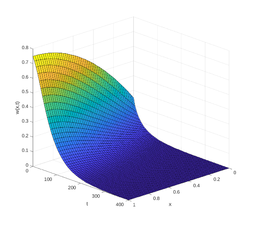
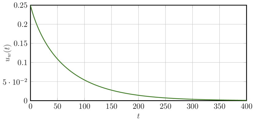
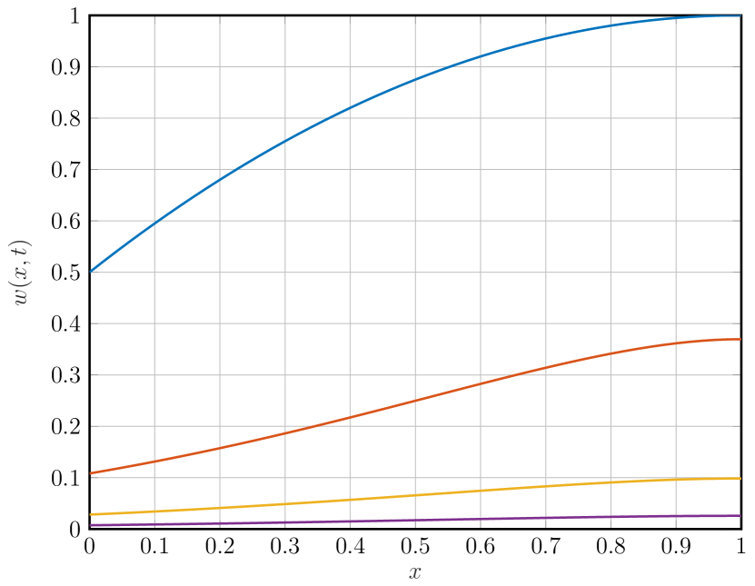
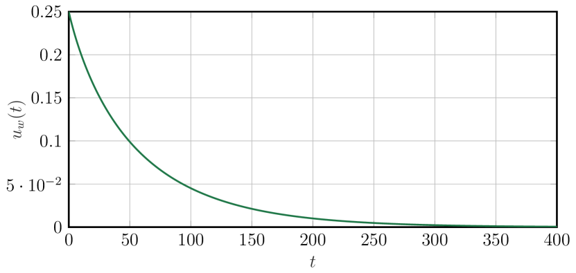
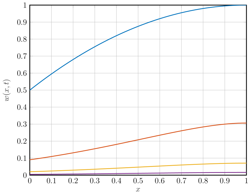
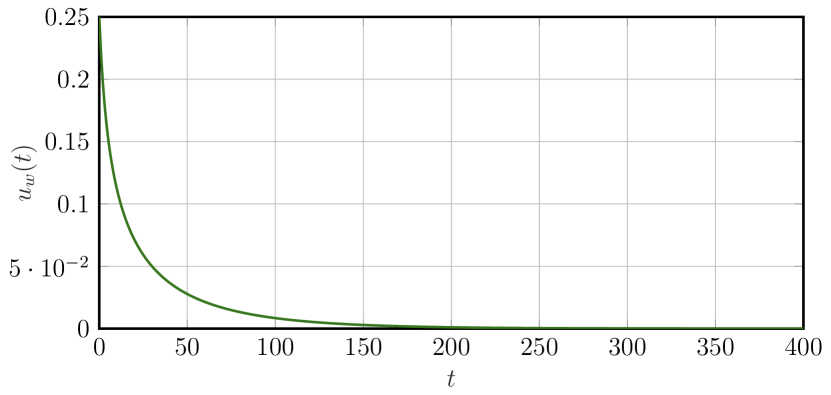
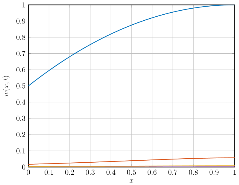
Refer to caption
Figure 1: 3D plot of $w(x,t)$ for $n=1$, $\alpha=0$.
Refer to caption
(a) Control function $u_{w}(t)$
Refer to caption
(b) Graphs of $x$-profiles of $w(x,t)$ at $t=0$ (blue), $t=100$ (orange), $t=200$ (yellow), and $t=300$ (purple)
Figure 2: Case $n=\frac{1}{2}$ and $\alpha=\frac{1}{2}$.
Refer to caption
(a) Control function $u_{w}(t)$
Refer to caption
(b) Graphs of $x$-profiles of $w(x,t)$ at $t=0$ (blue), $t=100$ (orange), $t=200$ (yellow), and $t=300$ (purple)
Figure 3: Case $n=2$ and $\alpha=\frac{1}{2}$.
Refer to caption
(a) Control function $u_{w}(t)$
Refer to caption
(b) Graphs of $x$-profiles of $w(x,t)$ at $t=0$ (blue), $t=100$ (orange), $t=200$ (yellow), and $t=300$ (purple)
Figure 4: Case $n=10$ and $\alpha=\frac{1}{2}$.

The solution profiles for $n=\frac{1}{2}$, $n=2$, and $n=10$ and the corresponding control functions defined by (3.4) are presented in Fig. 4, Fig. 4, and Fig. 4, respectively.

The presented plots illustrate the decay of solutions $w(x,t)$ for large values of $t$. To estimate the behavior of $w(x,t)$ over time, we use standard MATLAB R2019b functions to approximate the decay rate constant as follows:

$$\lambda_{N}=-\limsup_{t\to\infty}\frac{1}{t}\log\frac{\|w(\cdot,t)\|_{L^{2}_{\rho}(0,l)}}{\|w(\cdot,0)\|_{L^{2}_{\rho}(0,l)}},$$ (5.3)

within the time horizon $t\in[0\,s,7000\,s]$ using a discretization step of $1\,s$.

Table 1 summarizes the results of numerical computations of the decay rate constant $\lambda_{N}$ over the range $n\in\{\frac{1}{2},1,2,10\}$ and $\alpha\in\{0,\frac{1}{4},\frac{1}{2}\}$. These results enable us to compare the numerical values with the theoretical decay rate, defined in (4.8) as $\lambda_{T}=0.0025$ for the specific parameters given in (5.1).

Table 1: Estimated decay-rate $\lambda_{N}$ for different $\alpha$ and $n$
$\boldsymbol{n}$ $\boldsymbol{\alpha}$ $\boldsymbol{0}$ $\boldsymbol{1/4}$ $\boldsymbol{1/2}$
$\boldsymbol{1/2}$ $0.0045$ $0.0036$ $0.0039$
$\boldsymbol{1}$ $0.0038$ $0.0037$ $0.0035$
$\boldsymbol{2}$ $0.0042$ $0.0030$ $0.0026$
$\boldsymbol{10}$ $0.0039$ $0.0030$ $0.0027$

6 Conclusion

The mathematical model of $n^{th}$-order chemical reactions of the type “$A\to$ product” carried out in a dispersed flow tubular reactor (DFTR) has been studied. The dynamics are described by a nonlinear parabolic partial differential equation with feedback boundary control applied through variations of the inlet concentration. The abstract problem in operator form is presented and studied. A feedback control design is proposed to ensure the exponential stability of the steady-state solution to the problem. The existence and uniqueness of the solution to the initial value problem are proved under the proposed control.

The presented simulation results confirm the exponential decay of $w(x,t)$ for large values of $t$. Considering the chosen physical parameters, the profile of $w(x,t)$ closely approximates the steady-state value at $t=400\,s$, within an acceptable numerical tolerance.

The estimates of $\lambda_{N}$, presented in Table 1, exhibit nonlinear behavior with respect to each of the parameters $n$ and $\alpha$ over the given range. It is important to note that the theoretical decay rate estimate $\lambda_{T}=\frac{v^{2}}{16D_{ax}}$, obtained from the differential inequality (4.7), provides a lower bound for the estimates $\lambda_{N}$ in (5.3). Up to this point, there is no numerical evidence to indicate how accurate or sharp the estimate $\lambda_{T}$ in (4.6) is, as the data of Table 1 only addresses solutions with the specified initial condition (5.2). We leave the analysis of the sharpness of $\lambda_{T}$ for further studies. Another prospective topic for future research could focus on the input-to-state stability analysis of the problem expressed in equation (3.1).

References

  • [1] D.M. Bošković and M. Krstić. Backstepping control of chemical tubular reactors. Comput. Chem. Eng., 26(7-8):1077–1085, 2002. doi:10.1016/S0098-1354(02)00026-1.
  • [2] H. Brezis. Functional Analysis, Sobolev Spaces and Partial Differential Equations. Springer New York, NY, 2010.
  • [3] L. V. Kantorovich and G. P. Akilov. Functional Analysis. Elsevier, 2016.
  • [4] Xunjing Li and Jiongmin Yong. Optimal Control Theory for Infinite Dimensional Systems. Birkhäuser Boston, MA, 2012.
  • [5] E.B. Nauman and Ramesh Mallikarjun. Generalized boundary conditions for the axial dispersion model. Chem. Eng. J., 26(3):231–237, 1983. doi:10.1016/0300-9467(83)80018-5.
  • [6] A. Pazy. Semigroups of Linear Operators and Applications to Partial Differential Equations. Springer New York, NY, 2011.
  • [7] M. Petkovska and A. Seidel-Morgenstern. Evaluation of periodic processes. In P.L. Silveston and R.R. Hudgins, editors, ”Periodic Operation of Chemical Reactors”, chapter 14, pages 387–413. Butterworth-Heinemann, Oxford, 2013.
  • [8] J.-W. Wang, H.-N. Wu, and C.-Y. Sun. Boundary controller design and well-posedness analysis of semi-linear parabolic pde systems. In 2014 American Control Conference, pages 3369–3374, Portland, OR, USA, 2014.
  • [9] Jun-Wei Wang, Huai-Ning Wu, and Chang-Yin Sun. Local exponential stabilization via boundary feedback controllers for a class of unstable semi-linear parabolic distributed parameter processes. J. Frankl. Inst., 354(13):5221–5244, 2017. doi:10.1016/j.jfranklin.2017.05.044.
  • [10] Chengzhou Wei and Junmin Li. A generalized exponential stabilization for a class of semilinear parabolic equations: Linear boundary feedback control approach. Math. Methods Appl. Sci., 44(18):14677–14689, 2021. doi:10.1002/mma.7735.
  • [11] Y. Yevgenieva, A. Zuyev, P. Benner, and A. Seidel-Morgenstern. Periodic optimal control of a plug flow reactor model with an isoperimetric constraint. J. Optim. Theory Appl., 202:582–604, 2024. doi:10.1007/s10957-024-02439-w.
  • [12] A. Zuyev, A. Seidel-Morgenstern, and P. Benner. An isoperimetric optimal control problem for a non-isothermal chemical reactor with periodic inputs. Chem. Eng. Sci., 161:206–214, 2017. doi:10.1016/j.ces.2016.12.025.