Uncertainty quantification for electrical impedance tomography using quasi-Monte Carlo methods

Abstract

The theoretical development of quasi-Monte Carlo (QMC) methods for uncertainty quantification of partial differential equations (PDEs) is typically centered around simplified model problems such as elliptic PDEs subject to homogeneous zero Dirichlet boundary conditions. In this paper, we present a theoretical treatment of the application of randomly shifted rank-1 lattice rules to electrical impedance tomography (EIT). EIT is an imaging modality, where the goal is to reconstruct the interior conductivity of an object based on electrode measurements of current and voltage taken at the boundary of the object. This is an inverse problem, which we tackle using the Bayesian statistical inversion paradigm. As the reconstruction, we consider QMC integration to approximate the unknown conductivity given current and voltage measurements. We prove under moderate assumptions placed on the parameterization of the unknown conductivity that the QMC approximation of the reconstructed estimate has a dimension-independent, faster-than-Monte Carlo cubature convergence rate. Finally, we present numerical results for examples computed using simulated measurement data.

Keywords: Electrical impedance tomography, Bayesian inversion, complete electrode model, inaccurate measurement model, uncertainty quantification, quasi-Monte Carlo method

1 Introduction

Quasi-Monte Carlo (QMC) methods are a class of high-dimensional cubature rules with equal cubature weights. QMC methods have become a popular tool in the numerical treatment of uncertainties in partial differential equation (PDE) models with random or uncertain inputs. Studied topics include elliptic eigenvalue problems [1, 2], optimal control [3, 4], various diffusion problems [5, 6, 7], parametric operator equations [8, 9] as well as elliptic PDEs with random or lognormal coefficients [10, 11, 12, 13, 14, 15, 16, 17]. A common and sought-after advantage of these applications are the faster-than-Monte Carlo convergence rates of QMC methods and—under some moderate conditions—this convergence can be shown to be independent of the dimensionality of the associated integration problems. QMC methods are particularly well-suited to large-scale uncertainty quantification problems since it is typically easy to parallelize the computation over QMC point sets.

The overwhelming majority of QMC analyses for PDEs have been carried out within the context of the forward uncertainty quantification problem of approximating the expected value

$$\mathbb{E}[G(u)]=\int_{\Omega}G(u(\cdot,\omega))\,\mathbb{P}({\rm d}\omega),$$

where $(\Omega,\mathcal{A},\mathbb{P})$ is a probability space and $G$ is a bounded linear functional acting on the solution $u$ of an elliptic PDE with a random diffusion coefficient $a$ such as

$$\begin{cases}-\nabla\cdot(a({\boldsymbol{x}},\omega)\nabla u({\boldsymbol{x}},\omega))=f({\boldsymbol{x}}),&{\boldsymbol{x}}\in D,~{}\omega\in\Omega,\\ u({\boldsymbol{x}},\omega)=0,&{\boldsymbol{x}}\in\partial D,~{}\omega\in\Omega,\end{cases}$$ (1)

where $f\!:D\to\mathbb{R}$ is a fixed source term. For mathematical analysis, the boundary conditions are typically taken to be extremely simple such as the homogeneous zero Dirichlet boundary condition in (1), which is an unrealistic modeling assumption for most practical applications.

In addition, there have been some studies on Bayesian inversion governed by parametric PDEs [18, 19, 20, 21, 22, 23]. However, these studies generally restrict their attention to simplified model problems such as (1).

Meanwhile, electrical impedance tomography (EIT) is an imaging modality, which uses measurements of voltage and current taken over an array of electrodes placed on the boundary of an object, with the goal of reconstructing the unknown conductivity inside the object; see for example [24, 25]. The most accurate way to model the measurements of EIT is to employ the complete electrode model (CEM), which accounts for the electrode shapes and contact resistances caused by resistive layers at electrode-object interfaces [26, 27, 28]. The mathematical model of CEM is governed by an elliptic PDE—albeit one with more intricate boundary conditions than the problem (1)—which suggests that one can apply QMC theory for both forward and inverse uncertainty quantification for this problem. However, this kind of analysis does not appear to have been considered in the literature. It is the goal of this paper to rectify this situation.

This paper is organized as follows. We briefly review basic multi-index notation in Section 1.1. We define the problem setting—the so-called parametric complete electrode model—in Section 2. The parametric regularity analysis for both the forward model and inverse problem, i.e., the conditional mean estimator of the unknown conductivity, is carried out in Section 3. The basics of randomly shifted rank-1 lattice rules are discussed in Section 4, and the error analysis for the EIT problem is presented in Section 5. Numerical experiments are showcased in Section 6. Finally, some conclusions and future prospects are given in Section 7.

1.1 Notations and preliminaries

We will use boldfaced symbols to denote multi-indices while the subscript notation $\nu_{j}$ is used to refer to the $j^{\rm th}$ component of a multi-index $\boldsymbol{\nu}$. The set of finitely supported multi-indices is denoted by

$$\mathscr{F}:=\{\boldsymbol{\nu}\in\mathbb{N}_{0}^{\mathbb{N}}:|{\boldsymbol{\nu}}|<\infty\},$$

where the order of a multi-index $\boldsymbol{\nu}\in\mathscr{F}$ is defined as

$$|{\boldsymbol{\nu}}|:=\sum_{j\geq 1}\nu_{j}.$$

For any sequence ${\boldsymbol{x}}:=(x_{j})_{j\geq 1}$ of real numbers, we define

$${\boldsymbol{x}}^{\boldsymbol{\nu}}:=\prod_{j\geq 1}x_{j}^{\nu_{j}},$$

where we use the convention $0^{0}:=1$.

Let $\boldsymbol{m},{\boldsymbol{\nu}}\in\mathscr{F}$ be multi-indices. We define $\boldsymbol{m}\leq{\boldsymbol{\nu}}$ to mean $m_{j}\leq\nu_{j}$ for all $j\geq 1$. Finally, we define the shorthand notations

$$\partial_{{\boldsymbol{y}}}^{{\boldsymbol{\nu}}}:=\prod_{j\geq 1}\frac{\partial^{\nu_{j}}}{\partial y_{j}^{\nu_{j}}}\quad\text{and}\quad\binom{{\boldsymbol{\nu}}}{\boldsymbol{m}}:=\prod_{j\geq 1}\binom{\nu_{j}}{m_{j}}.$$

2 Parametric complete electrode model

Let $D\subset\mathbb{R}^{d}$, $d\in\{1,2,3\}$, denote a nonempty, bounded physical domain with Lipschitz boundary and let $\Upsilon:=(-1/2,1/2)^{\mathbb{N}}$ denote a set of parameters. We state the following assumptions about the parametric conductivity field.

Assumption 2.1.

The parametric conductivity coefficient $a\!:D\times\Upsilon\to\mathbb{R}$ satisfies the following assumptions: [1em]0em

1. $a(\cdot,{\boldsymbol{y}})\in L^{\infty}(D)$ for all ${\boldsymbol{y}}\in\Upsilon$.

2. There exist constants $C_{a},\sigma\geq 1$ and a sequence $\boldsymbol{\rho}=(\rho_{j})_{j\geq 1}\in\ell^{1}(\mathbb{N})$ of non-negative real numbers such that

   $$\|\partial_{{\boldsymbol{y}}}^{{\boldsymbol{\nu}}}a(\cdot,{\boldsymbol{y}})\|_{L^{\infty}(D)}\leq C_{a}(|{\boldsymbol{\nu}}|!)^{\sigma}\boldsymbol{\rho}^{{\boldsymbol{\nu}}}\quad\text{for all}~{}{\boldsymbol{\nu}}\in\mathscr{F}~{}\text{and}~{}{\boldsymbol{y}}\in\Upsilon.$$

3. There exist positive constants $a_{\min}$ and $a_{\max}$ such that

   $$0<a_{\min}\leq a({\boldsymbol{x}},{\boldsymbol{y}})\leq a_{\max}<\infty\quad\text{for all ${\boldsymbol{x}}\in D$ and ${\boldsymbol{y}}\in\Upsilon$.}$$

Assumptions (A1) and (A3) ensure that the coefficient $a$ is uniformly elliptic over the parameter domain $\Upsilon$. Meanwhile, assumption (A2) asserts that $a$ belongs to the Gevrey class with parameter $\sigma$ with respect to the variable ${\boldsymbol{y}}\in\Upsilon$. This class has recently been studied within the context of forward uncertainty quantification for elliptic PDEs [1, 5, 29]. The Gevrey class covers a wider range of possible parameterizations for the input random field $a$, which enable the development of dimension-robust QMC cubatures for uncertainty quantification.

Let $\{E_{k}\}_{k=1}^{M}$, $M\geq 2$, be open, nonempty, connected subsets of $D$ such that $\overline{E}_{i}\cap\overline{E}_{j}=\varnothing$ for $i\neq j$. We define the quotient Hilbert space $\mathcal{H}:=(H^{1}(D)\oplus\mathbb{R}^{M})/\mathbb{R}$, endowed with the norm

$$\|(v,V)\|_{\mathcal{H}}^{2}:=\int_{D}|\nabla v|^{2}\,{\rm d}{\boldsymbol{x}}+\sum_{k=1}^{M}\int_{E_{k}}(v-V_{m})^{2}\,{\rm d}S,\quad(v,V)\in\mathcal{H}.$$

Note that $(u,U)=(v,V)\in\mathcal{H}$, if

$$u-v={\rm constant}=U_{1}-V_{1}=\cdots=U_{M}-V_{M}.$$

Let $a\!:D\times\Upsilon\to\mathbb{R}$ be a parametric conductivity field satisfying Assumption 2.1. The forward problem is to find, for ${\boldsymbol{y}}\in\Upsilon$, the electromagnetic potential $u(\cdot,{\boldsymbol{y}})$ and the potentials on the electrodes $U({\boldsymbol{y}})$ satisfying

$$\begin{cases}\nabla\cdot(a(\cdot,{\boldsymbol{y}})\nabla u(\cdot,{\boldsymbol{y}}))=0&\text{in}~{}D,\\ a(\cdot,{\boldsymbol{y}})\frac{\partial u(\cdot,{\boldsymbol{y}})}{\partial\boldsymbol{n}}=0&\text{on}~{}\partial D\setminus\overline{E},\\ u(\cdot,{\boldsymbol{y}})+z_{m}a(\cdot,{\boldsymbol{y}})\frac{\partial u(\cdot,{\boldsymbol{y}})}{\partial\boldsymbol{n}}=U_{m}({\boldsymbol{y}})&\text{on}~{}E_{m},~{}m\in\{1,\ldots,M\},\\ \int_{E_{m}}a({\boldsymbol{x}},{\boldsymbol{y}})\frac{\partial u({\boldsymbol{x}},{\boldsymbol{y}})}{\partial\boldsymbol{n}}\,{\rm d}S({\boldsymbol{x}})=I_{m}&m\in\{1,\ldots,M\},\end{cases}$$

where $\boldsymbol{n}=\boldsymbol{n}({\boldsymbol{x}})$ denotes the outward pointing unit normal vector for ${\boldsymbol{x}}\in\partial D$, the vector $I\in\mathbb{R}^{M}$ consists of the net current feed through the electrodes with $\sum_{m=1}^{M}I_{m}=0$, and the real-valued contact impedances $\{z_{m}\}_{m=1}^{M}$ are assumed to satisfy, for some positive constants $\varsigma_{-}$ and $\varsigma_{+}$, the inequalities $0<\varsigma_{-}\leq z_{m}\leq\varsigma_{+}<\infty$ for all $m\in\{1,\ldots,M\}$.

The variational formulation of the above is: for ${\boldsymbol{y}}\in\Upsilon$, find $(u(\cdot,{\boldsymbol{y}}),U({\boldsymbol{y}}))\in\mathcal{H}$ such that

$$B((u(\cdot,{\boldsymbol{y}}),U(\cdot,{\boldsymbol{y}})),(v,V))=\sum_{m=1}^{M}I_{m}V_{m}$$ (2)

for all $(v,V)\in\mathcal{H}$, where

$$B((w,W),(v,V))=\int_{D}a(\cdot,{\boldsymbol{y}})\nabla w\cdot\nabla v\,{\rm d}{\boldsymbol{x}}+\sum_{m=1}^{M}\frac{1}{z_{m}}\int_{E_{m}}(w-W_{m})(v-V_{m})\,{\rm d}S.$$

It is known that, under the aforementioned assumptions, a unique solution to the variational formulation exists [28]. Moreover, the solution satisfies the a priori bound (cf. [30, Lemma 2.1])

$$\|(u(\cdot,{\boldsymbol{y}}),U({\boldsymbol{y}}))\|_{\mathcal{H}}\leq\frac{C|I|}{\min\{a_{\min},\varsigma_{+}^{-1}\}}\quad\text{for all}~{}{\boldsymbol{y}}\in\Upsilon,$$

where $C>0$ is a constant depending on $D$ and $E$. We call the model (2) the parametric complete electrode model (pCEM). The pCEM was introduced in the numerical study [31], but analytic properties such as parametric regularity were not investigated.

3 Parametric regularity

3.1 Forward problem

We begin by establishing the existence of the higher-order partial derivatives of the solution to (2). The following lemma shows that the first-order partial derivatives are well-defined. To this end, we generalize the proof strategy of [32, Theorem 4.2] for nonlinear parameterizations of the input coefficient $a$.

Lemma 3.1.

Let Assumption 2.1 hold and let $(u(\cdot,{\boldsymbol{y}}),U({\boldsymbol{y}}))\in\mathcal{H}$ be the solution to (2). Then $\partial_{y_{j}}(u(\cdot,{\boldsymbol{y}}),U({\boldsymbol{y}}))$ exists and belongs to $\mathcal{H}$ for all $j\geq 1$ and ${\boldsymbol{y}}\in\Upsilon$.

Proof.

Let $\boldsymbol{e}_{j}$ denote the unit vector with $1$ at index $j$ and $0$ otherwise. For $h\in\mathbb{R}\setminus\{0\}$ define the difference quotients

$$w_{h}(\cdot,{\boldsymbol{y}}) :=\frac{u(\cdot,{\boldsymbol{y}}+h\boldsymbol{e}_{j})-u(\cdot,{\boldsymbol{y}})}{h},$$

$$W_{h}({\boldsymbol{y}}) :=\frac{U({\boldsymbol{y}}+h\boldsymbol{e}_{j})-U({\boldsymbol{y}})}{h},$$

$$\alpha_{h}(\cdot,{\boldsymbol{y}}) :=\frac{a(\cdot,{\boldsymbol{y}}+h\boldsymbol{e}_{j})-a(\cdot,{\boldsymbol{y}})}{h}.$$

For sufficiently small $|h|<1$,

$$a_{\min}\leq a({\boldsymbol{x}},{\boldsymbol{y}}+h\boldsymbol{e}_{j})\leq a_{\max},\quad{\boldsymbol{x}}\in D,$$

which means that $u(\cdot,{\boldsymbol{y}}+h\boldsymbol{e}_{j})$ is well-defined as an element of $\mathcal{H}$. Then we can conclude that for all $(v,V)\in\mathcal{H}$, there holds

$$0 =\int_{D}a({\boldsymbol{x}},{\boldsymbol{y}}+h\boldsymbol{e}_{j})\nabla u({\boldsymbol{x}},{\boldsymbol{y}}+h\boldsymbol{e}_{j})\cdot\nabla v({\boldsymbol{x}})\,{\rm d}{\boldsymbol{x}}\!-\!\int_{D}a({\boldsymbol{x}},{\boldsymbol{y}})\nabla u({\boldsymbol{x}},{\boldsymbol{y}}+h\boldsymbol{e}_{j})\cdot\nabla v({\boldsymbol{x}})\,{\rm d}{\boldsymbol{x}}$$

$$\quad+\int_{D}a({\boldsymbol{x}},{\boldsymbol{y}})\nabla u({\boldsymbol{x}},{\boldsymbol{y}}+h\boldsymbol{e}_{j})\cdot\nabla v({\boldsymbol{x}})\,{\rm d}{\boldsymbol{x}}-\int_{D}a({\boldsymbol{x}},{\boldsymbol{y}})\nabla u({\boldsymbol{x}},{\boldsymbol{y}})\cdot\nabla v({\boldsymbol{x}})\,{\rm d}{\boldsymbol{x}}$$

$$\quad+\sum_{m=1}^{M}\frac{1}{z_{m}}\int_{E_{m}}((u({\boldsymbol{x}},{\boldsymbol{y}}+h\boldsymbol{e}_{j})-u({\boldsymbol{x}},{\boldsymbol{y}}))-((U({\boldsymbol{y}}+h\boldsymbol{e}_{j})-U({\boldsymbol{y}})))(v({\boldsymbol{x}})-V)\,{\rm d}S({\boldsymbol{x}})$$

$$=h\int_{D}\alpha_{h}({\boldsymbol{x}},{\boldsymbol{y}})\nabla u({\boldsymbol{x}},{\boldsymbol{y}}+h\boldsymbol{e}_{j})\cdot\nabla v({\boldsymbol{x}})\,{\rm d}{\boldsymbol{x}}+h\int_{D}a({\boldsymbol{x}},{\boldsymbol{y}})\nabla w_{h}({\boldsymbol{x}},{\boldsymbol{y}})\cdot\nabla v({\boldsymbol{x}})\,{\rm d}{\boldsymbol{x}}$$

$$\quad+h\sum_{m=1}^{M}\frac{1}{z_{m}}\int_{E_{m}}(w_{h}({\boldsymbol{x}},{\boldsymbol{y}})-W_{h}({\boldsymbol{y}}))(v({\boldsymbol{x}})-V)\,{\rm d}S({\boldsymbol{x}}).$$

We can rewrite this as

$$B((w_{h}(\cdot,{\boldsymbol{y}}),W_{h}(\cdot,{\boldsymbol{y}})),(v,V))=L_{h}((v,V)),$$

where $L_{h}\!:\mathcal{H}\to\mathbb{R}$, $L_{h}((v,V)):=-\int_{D}\alpha_{h}({\boldsymbol{x}},{\boldsymbol{y}})\nabla u({\boldsymbol{x}},{\boldsymbol{y}}+h\boldsymbol{e}_{j})\cdot\nabla v({\boldsymbol{x}})\,{\rm d}{\boldsymbol{x}}$, is a linear functional. Analogously to  [32, Theorem 4.2] one can show that $L_{h}$ converges to $L_{0}$ in $\mathcal{H}$ as $h\rightarrow 0$. Therefore $(w_{h},W_{h})$ converges to $(w_{0},W_{0})$, which is the solution to

$$\int_{D}a({\boldsymbol{x}},{\boldsymbol{y}})\nabla w_{0}({\boldsymbol{x}},{\boldsymbol{y}})\cdot\nabla v({\boldsymbol{x}})\,{\rm d}{\boldsymbol{x}}+\sum_{m=1}^{M}\frac{1}{z_{m}}\int_{E_{m}}(w_{0}(\cdot,{\boldsymbol{y}})-W_{0}({\boldsymbol{y}}))(v-V_{m})\,{\rm d}S=L_{0}(v).$$

Hence $\partial_{y_{j}}(u(\cdot,{\boldsymbol{y}}),U({\boldsymbol{y}}))=(w_{0},W_{0})$ exists in $\mathcal{H}$ and is the unique solution of the variational problem

$$\int_{D}a({\boldsymbol{x}},{\boldsymbol{y}})\nabla\partial_{y_{j}}u({\boldsymbol{x}},{\boldsymbol{y}})\cdot\nabla v({\boldsymbol{x}})\,{\rm d}{\boldsymbol{x}}+\sum_{m=1}^{M}\frac{1}{z_{m}}\int_{E_{m}}(\partial_{y_{j}}u(\cdot,{\boldsymbol{y}})-\partial_{y_{j}}U({\boldsymbol{y}}))(v-V_{m})\,{\rm d}S$$

$$=-\int_{D}\partial_{y_{j}}a({\boldsymbol{x}},{\boldsymbol{y}})\nabla u({\boldsymbol{x}},{\boldsymbol{y}})\cdot\nabla v({\boldsymbol{x}})\,{\rm d}{\boldsymbol{x}}$$

for all $(v,V)\in\mathcal{H}$. This concludes the proof. ∎

By inductive reasoning, we obtain the existence of higher-order partial derivatives as a corollary.

Corollary 3.2.

Let the assumptions of Lemma 3.1 hold. Then $\partial_{{\boldsymbol{y}}}^{{\boldsymbol{\nu}}}(u(\cdot,{\boldsymbol{y}}),U({\boldsymbol{y}}))$ exists and belongs to $\mathcal{H}$ for all ${\boldsymbol{\nu}}\in\mathscr{F}$ and ${\boldsymbol{y}}\in\Upsilon$.

Corollary 3.2 enables us to obtain the higher-order partial derivatives of the solution to (2) by formally differentiating the variational formulation on both sides with respect to the parametric variable. This yields the following recursive bound for the higher-order partial derivatives.

Lemma 3.3 (Recursive bound).

Let the assumptions of Lemma 3.1 hold. Let ${\boldsymbol{\nu}}\in\mathscr{F}\setminus\{\mathbf{0}\}$ and ${\boldsymbol{y}}\in\Upsilon$. Then

$$\|\partial_{{\boldsymbol{y}}}^{{\boldsymbol{\nu}}}(u(\cdot,{\boldsymbol{y}}),U(\cdot,{\boldsymbol{y}}))\|_{\mathcal{H}}\leq\frac{C_{a}}{\min\{a_{\min},\varsigma_{+}^{-1}\}}\!\sum_{\mathbf{0}\neq\boldsymbol{m}\leq{\boldsymbol{\nu}}}\!\binom{{\boldsymbol{\nu}}}{\boldsymbol{m}}(|\boldsymbol{m}|!)^{\sigma}\boldsymbol{\rho}^{\boldsymbol{m}}\|\partial_{\boldsymbol{y}}^{{\boldsymbol{\nu}}-\boldsymbol{m}}(u(\cdot,{\boldsymbol{y}}),U({\boldsymbol{y}}))\|_{\mathcal{H}}.$$

Proof.

We differentiate the variational formulation (2) on both sides with respect to ${\boldsymbol{y}}\in\Upsilon$ and use the Leibniz product rule, which yields

$$\int_{D}a({\boldsymbol{x}},{\boldsymbol{y}})\nabla\partial_{{\boldsymbol{y}}}^{{\boldsymbol{\nu}}}u({\boldsymbol{x}},{\boldsymbol{y}})\cdot\nabla v({\boldsymbol{x}})\,{\rm d}{\boldsymbol{x}}$$

$$\quad+\sum_{m=1}^{M}\frac{1}{z_{m}}\int_{E_{m}}(\partial_{\boldsymbol{y}}^{{\boldsymbol{\nu}}}u({\boldsymbol{x}},{\boldsymbol{y}})-\partial_{{\boldsymbol{y}}}^{{\boldsymbol{\nu}}}U({\boldsymbol{x}},{\boldsymbol{y}}))(v({\boldsymbol{x}})-V({\boldsymbol{x}}))\,{\rm d}S({\boldsymbol{x}})$$

$$=-\sum_{\mathbf{0}\neq\boldsymbol{m}\leq{\boldsymbol{\nu}}}\binom{{\boldsymbol{\nu}}}{\boldsymbol{m}}\int_{D}\partial_{{\boldsymbol{y}}}^{\boldsymbol{m}}a({\boldsymbol{x}},{\boldsymbol{y}})\nabla\partial_{{\boldsymbol{y}}}^{{\boldsymbol{\nu}}-\boldsymbol{m}}u({\boldsymbol{x}},{\boldsymbol{y}})\cdot\nabla v({\boldsymbol{x}})\,{\rm d}{\boldsymbol{x}}.$$

Setting $(v,V)=(\partial_{{\boldsymbol{y}}}^{{\boldsymbol{\nu}}}u(\cdot,{\boldsymbol{y}}),\partial_{{\boldsymbol{y}}}^{{\boldsymbol{\nu}}}U({\boldsymbol{y}}))\in\mathcal{H}$, we obtain

$$\min\{a_{\min},\varsigma_{+}^{-1}\}\|(\partial_{{\boldsymbol{y}}}^{{\boldsymbol{\nu}}}u(\cdot,{\boldsymbol{y}}),\partial_{{\boldsymbol{y}}}^{{\boldsymbol{\nu}}}U(\cdot,{\boldsymbol{y}}))\|_{\mathcal{H}}^{2}$$

$$\leq\int_{D}a({\boldsymbol{x}},{\boldsymbol{y}})|\nabla\partial_{{\boldsymbol{y}}}^{{\boldsymbol{\nu}}}u({\boldsymbol{x}},{\boldsymbol{y}})|^{2}\,{\rm d}{\boldsymbol{x}}+\sum_{m=1}^{M}\frac{1}{z_{m}}\int_{E_{m}}(\partial_{\boldsymbol{y}}^{{\boldsymbol{\nu}}}u({\boldsymbol{x}},{\boldsymbol{y}})-\partial_{{\boldsymbol{y}}}^{{\boldsymbol{\nu}}}U({\boldsymbol{y}}))^{2}\,{\rm d}S({\boldsymbol{x}})$$

$$=-\sum_{\mathbf{0}\neq\boldsymbol{m}\leq{\boldsymbol{\nu}}}\binom{{\boldsymbol{\nu}}}{\boldsymbol{m}}\int_{D}\partial_{{\boldsymbol{y}}}^{\boldsymbol{m}}a({\boldsymbol{x}},{\boldsymbol{y}})\nabla\partial_{{\boldsymbol{y}}}^{{\boldsymbol{\nu}}-\boldsymbol{m}}u({\boldsymbol{x}},{\boldsymbol{y}})\cdot\nabla\partial_{{\boldsymbol{y}}}^{{\boldsymbol{\nu}}}u({\boldsymbol{x}},{\boldsymbol{y}})\,{\rm d}{\boldsymbol{x}}$$

$$\leq\sum_{\mathbf{0}\neq\boldsymbol{m}\leq{\boldsymbol{\nu}}}\binom{{\boldsymbol{\nu}}}{\boldsymbol{m}}\|\partial_{{\boldsymbol{y}}}^{\boldsymbol{m}}a(\cdot,{\boldsymbol{y}})\|_{L^{\infty}(D)}\bigg{(}\int_{D}|\nabla\partial_{{\boldsymbol{y}}}^{{\boldsymbol{\nu}}-\boldsymbol{m}}u({\boldsymbol{x}},{\boldsymbol{y}})|^{2}\,{\rm d}{\boldsymbol{x}}\bigg{)}^{\frac{1}{2}}\!\bigg{(}\int_{D}|\nabla\partial_{{\boldsymbol{y}}}^{{\boldsymbol{\nu}}}u({\boldsymbol{x}},{\boldsymbol{y}})|^{2}\,{\rm d}{\boldsymbol{x}}\bigg{)}^{\frac{1}{2}}$$

$$\leq\sum_{\mathbf{0}\neq\boldsymbol{m}\leq{\boldsymbol{\nu}}}\binom{{\boldsymbol{\nu}}}{\boldsymbol{m}}C_{a}(|\boldsymbol{m}|!)^{\sigma}\boldsymbol{\rho}^{\boldsymbol{m}}\|\partial_{\boldsymbol{y}}^{{\boldsymbol{\nu}}-\boldsymbol{m}}(u(\cdot,{\boldsymbol{y}}),U({\boldsymbol{y}}))\|_{\mathcal{H}}\|\partial_{\boldsymbol{y}}^{{\boldsymbol{\nu}}}(u(\cdot,{\boldsymbol{y}}),U({\boldsymbol{y}}))\|_{\mathcal{H}},$$

where we applied (A2). The result follows by canceling the common factor on both sides and dividing both sides of the inequality by $\min\{a_{\min},\varsigma_{+}^{-1}\}$. ∎

In consequence, the recursive bound allows us to derive an a priori bound on the higher-order partial derivatives. To this end, we will make use of the following result for multivariable recurrence relations.

Lemma 3.4 (cf. [33, Lemma 3.1]).

Let $(\Xi_{{\boldsymbol{\nu}}})_{{\boldsymbol{\nu}}\in\mathscr{F}}$ and ${\boldsymbol{b}}=(b_{j})_{j\geq 1}$ be sequences satisfying

$$\Xi_{\mathbf{0}}\leq c_{0}\quad\text{and}\quad\Xi_{{\boldsymbol{\nu}}}\leq c\sum_{\begin{subarray}{c}\boldsymbol{m}\leq{\boldsymbol{\nu}}\\ \boldsymbol{m}\neq\mathbf{0}\end{subarray}}\binom{{\boldsymbol{\nu}}}{\boldsymbol{m}}(|\boldsymbol{m}|!)^{\sigma}\boldsymbol{b}^{\boldsymbol{m}}\Xi_{{\boldsymbol{\nu}}-\boldsymbol{m}}\quad\text{for all}~{}{\boldsymbol{\nu}}\in\mathscr{F}\setminus\{\mathbf{0}\},$$

where $c_{0},c>0$ and $\sigma\geq 1$. Then there holds

$$\Xi_{{\boldsymbol{\nu}}}\leq c_{0}c^{1-\delta_{|{\boldsymbol{\nu}}|,0}}(c+1)^{\max\{|{\boldsymbol{\nu}}|-1,0\}}(|{\boldsymbol{\nu}}|!)^{\sigma}\boldsymbol{b}^{{\boldsymbol{\nu}}}.$$

Lemma 3.4 immediately yields the following result when applied to the recurrence relation in Lemma 3.3.

Lemma 3.5 (Inductive bound).

Let the assumptions of Lemma 3.1 hold. Let ${\boldsymbol{\nu}}\in\mathscr{F}\setminus\{\mathbf{0}\}$ and ${\boldsymbol{y}}\in\Upsilon$. Then

$$\|\partial^{{\boldsymbol{\nu}}}(u(\cdot,{\boldsymbol{y}}),U({\boldsymbol{y}}))\|_{\mathcal{H}}\leq C_{u}(|{\boldsymbol{\nu}}|!)^{\sigma}\boldsymbol{b}^{{\boldsymbol{\nu}}},$$

where

$$C_{u}=\frac{C|I|}{\min\{a_{\min},\varsigma_{+}^{-1}\}}~{}\text{and}~{}b_{j}:=\bigg{(}1+\frac{C_{a}}{\min\{a_{\min},\varsigma_{+}^{-1}\}}\bigg{)}\rho_{j}.$$

3.2 Bayesian inverse problem

In what follows, we truncate the parametric domain $\Upsilon$ to $(-1/2,1/2)^{s}$. We shall further assume, for all ${\boldsymbol{y}}\in(-1/2,1/2)^{s}$, that ${\boldsymbol{x}}\mapsto a({\boldsymbol{x}},{\boldsymbol{y}})$ is well-defined over $\overline{D}$. Bayesian inference can be used to express the solution to an inverse problem in terms of a high-dimensional posterior distribution. Specifically, we assume that we have some voltage measurements taken at the $M$ electrodes placed on the boundary of the computational domain $D$ corresponding to the observation operator $\mathcal{O}\!:(-1/2,1/2)^{s}\to\mathbb{R}^{M}$,

$$\mathcal{O}({\boldsymbol{y}}):=[U_{1}({\boldsymbol{y}}),\ldots,U_{M}({\boldsymbol{y}})]^{\rm T}.$$

Furthermore, we assume that the observations are contaminated with additive Gaussian noise, leading to the measurement model

$$\boldsymbol{\delta}=\mathcal{O}({\boldsymbol{y}})+\boldsymbol{\eta},$$

where $\boldsymbol{\delta}\in\mathbb{R}^{M}$ are the noisy voltage measurements, $\mathcal{O}$ is the observation operator, ${\boldsymbol{y}}\in(-1/2,1/2)^{s}$ is the unknown parameter, and $\boldsymbol{\eta}\in\mathbb{R}^{M}$ is a realization of additive Gaussian noise.

We endow ${\boldsymbol{y}}$ with the uniform prior distribution $\mathcal{U}((-1/2,1/2)^{s})$, assume that ${\boldsymbol{\eta}}\sim\mathcal{N}(0,\Gamma)$, where $\Gamma\in\mathbb{R}^{M\times M}$ is a symmetric, positive definite covariance matrix, and that ${\boldsymbol{y}}$ and ${\boldsymbol{\eta}}$ are independent. Then the posterior distribution can be expressed by applying Bayes’ theorem and is given by

$$\pi({\boldsymbol{y}}\mid\boldsymbol{\delta})=\frac{\pi(\boldsymbol{\delta}\mid{\boldsymbol{y}})\pi_{\rm pr}({\boldsymbol{y}})}{Z(\boldsymbol{\delta})},$$

where $\pi_{\rm pr}({\boldsymbol{y}})=\chi_{(-1/2,1/2)^{s}}({\boldsymbol{y}})$, we define the unnormalized likelihood by

$$\pi(\boldsymbol{\delta}\mid{\boldsymbol{y}})\propto{\rm e}^{-\frac{1}{2}(\boldsymbol{\delta}-\mathcal{O}({\boldsymbol{y}}))^{\rm T}\Gamma^{-1}(\boldsymbol{\delta}-\mathcal{O}({\boldsymbol{y}}))},$$

and $Z(\boldsymbol{\delta}):=\int_{(-1/2,1/2)^{s}}\pi(\boldsymbol{\delta}\,|\,{\boldsymbol{y}})\,{\rm d}{\boldsymbol{y}}$. As our estimator of the unknown parameter ${\boldsymbol{y}}\in(-1/2,1/2)^{s}$, we consider the quantity of interest

$$\widehat{a}=\frac{Z^{\prime}(\boldsymbol{\delta})}{Z(\boldsymbol{\delta})},\quad Z^{\prime}(\boldsymbol{\delta}):=\int_{(-1/2,1/2)^{s}}a({\boldsymbol{x}},{\boldsymbol{y}})\,\pi(\boldsymbol{\delta}\mid{\boldsymbol{y}})\,{\rm d}{\boldsymbol{y}}.$$ (3)

To obtain a parametric regularity bound for the normalization constant $Z(\boldsymbol{\delta})$, there holds by Lemma 3.5 and the trace theorem [34] that

$$\|\partial_{{\boldsymbol{y}}}^{{\boldsymbol{\nu}}}\mathcal{O}({\boldsymbol{y}})\|_{\mathbb{R}^{M}}\leq\frac{1}{2}C_{\rm init}(|{\boldsymbol{\nu}}|!)^{\sigma}{\boldsymbol{b}}^{{\boldsymbol{\nu}}},$$

where the constant $C_{\rm init}>0$ is defined as

$$C_{\rm init}:=2C_{u}\cdot\|\gamma\|_{H^{1}(D)\to L^{2}(\partial D)},$$

with $C_{u}$ defined in Lemma (3.5) and $\|\gamma\|_{H^{1}(D)\to L^{2}(\partial D)}$ is the norm of the trace operator $\gamma\!:H^{1}(D)\to L^{2}(\partial D)$, which depends on $D$ and $E$.

A parametric regularity bound for $Z(\boldsymbol{\delta})$ can be obtained as a consequence of [35, Lemma 5.3].

Lemma 3.6.

Let the assumptions of Lemma 3.1 hold. Let ${\boldsymbol{\nu}}\in\mathbb{N}_{0}^{s}$ and ${\boldsymbol{y}}\in(-1/2,1/2)^{s}$. Then

$$|\partial_{{\boldsymbol{y}}}^{{\boldsymbol{\nu}}}\pi(\boldsymbol{\delta}\mid{\boldsymbol{y}})|\leq\frac{1}{2}\cdot 3.82^{M}C_{\rm init}^{|{\boldsymbol{\nu}}|}\mu_{\min}^{-\frac{|{\boldsymbol{\nu}}|}{2}}(|{\boldsymbol{\nu}}|!)^{\sigma}\boldsymbol{b}^{{\boldsymbol{\nu}}},$$

where $0<\mu_{\min}\leq 1$ is a lower bound on the smallest eigenvalue of $\Gamma$.

For the parametric regularity of the term $Z^{\prime}(\boldsymbol{\delta})$, we obtain the following result.

Lemma 3.7.

Let the assumptions of Lemma 3.1 hold. Let ${\boldsymbol{\nu}}\in\mathbb{N}_{0}^{s}$ and ${\boldsymbol{y}}\in(-1/2,1/2)^{s}$. Then

$$|\partial_{{\boldsymbol{y}}}^{{\boldsymbol{\nu}}}(a({\boldsymbol{x}},{\boldsymbol{y}})\pi(\boldsymbol{\delta}\mid{\boldsymbol{y}}))|\leq\frac{C_{a}}{2}\cdot 3.82^{M}((|{\boldsymbol{\nu}}|+1)!)^{\sigma}\boldsymbol{\beta}^{{\boldsymbol{\nu}}},$$

where $0<\mu_{\min}\leq 1$ is a lower bound on the smallest eigenvalue of $\Gamma$ and we define the sequence $\boldsymbol{\beta}=(\beta_{j})_{j\geq 1}$ by setting

$$\beta_{j}:=\max\{1,C_{\rm init}\}\bigg{(}1+\frac{C_{a}}{\min\{a_{\min},\varsigma_{+}^{-1}\}}\bigg{)}\mu_{\min}^{-\frac{1}{2}}\rho_{j}.$$ (4)

Proof.

Let ${\boldsymbol{\nu}}\in\mathscr{F}\setminus\{\mathbf{0}\}$. The Leibniz product rule yields

$$\partial_{{\boldsymbol{y}}}^{{\boldsymbol{\nu}}}\big{(}a({\boldsymbol{x}},{\boldsymbol{y}}){\rm e}^{-\frac{1}{2}(\boldsymbol{\delta}-\mathcal{O}({\boldsymbol{y}}))^{\rm T}\Gamma^{-1}(\boldsymbol{\delta}-\mathcal{O}({\boldsymbol{y}}))}\big{)}$$

$$=\, \sum_{\boldsymbol{m}\leq{\boldsymbol{\nu}}}\binom{{\boldsymbol{\nu}}}{\boldsymbol{m}}\partial_{{\boldsymbol{y}}}^{\boldsymbol{m}}a({\boldsymbol{x}},{\boldsymbol{y}})\partial_{{\boldsymbol{y}}}^{{\boldsymbol{\nu}}-\boldsymbol{m}}{\rm e}^{-\frac{1}{2}(\boldsymbol{\delta}-\mathcal{O}({\boldsymbol{y}}))^{\rm T}\Gamma^{-1}(\boldsymbol{\delta}-\mathcal{O}({\boldsymbol{y}}))}$$

$$\leq\, \frac{1}{2}\cdot 3.82^{M}C_{a}\bigg{(}\max\{1,C_{\rm init}\}\bigg{(}1+\frac{C_{a}}{\min\{a_{\min},\varsigma_{+}^{-1}\}}\bigg{)}\mu_{\min}^{-\frac{1}{2}}\bigg{)}^{|{\boldsymbol{\nu}}|}\boldsymbol{\rho}^{{\boldsymbol{\nu}}}$$

$$\quad\times\sum_{\boldsymbol{m}\leq{\boldsymbol{\nu}}}\binom{{\boldsymbol{\nu}}}{\boldsymbol{m}}(|\boldsymbol{m}|!)^{\sigma}((|{\boldsymbol{\nu}}|-|\boldsymbol{m}|)!)^{\sigma}.$$

The claim follows by noting that

$$\sum_{\boldsymbol{m}\leq{\boldsymbol{\nu}}}\binom{{\boldsymbol{\nu}}}{\boldsymbol{m}}(|\boldsymbol{m}|!)^{\sigma}((|{\boldsymbol{\nu}}|-|\boldsymbol{m}|)!)^{\sigma}=\sum_{\ell=0}^{|{\boldsymbol{\nu}}|}(\ell!)^{\sigma}((|{\boldsymbol{\nu}}|-\ell)!)^{\sigma}\sum_{\begin{subarray}{c}\boldsymbol{m}\leq{\boldsymbol{\nu}}\\ |\boldsymbol{m}|=\ell\end{subarray}}\binom{{\boldsymbol{\nu}}}{\boldsymbol{m}}$$

$$=\sum_{\ell=0}^{|{\boldsymbol{\nu}}|}(\ell!)^{\sigma}((|{\boldsymbol{\nu}}|-\ell)!)^{\sigma}\binom{|{\boldsymbol{\nu}}|}{\ell}=|{\boldsymbol{\nu}}|!\sum_{\ell=0}^{|{\boldsymbol{\nu}}|}(\ell!)^{\sigma-1}((|{\boldsymbol{\nu}}|-\ell)!)^{\sigma-1}$$

$$\leq|{\boldsymbol{\nu}}|!\sum_{\ell=0}^{|{\boldsymbol{\nu}}|}(|{\boldsymbol{\nu}}|!)^{\sigma-1}=(|{\boldsymbol{\nu}}|!)^{\sigma}(|{\boldsymbol{\nu}}|+1)\leq((|{\boldsymbol{\nu}}|+1)!)^{\sigma},$$

where we used the fact that $\ell!(v-\ell)!\leq v!$ for natural numbers $v\geq\ell$ and that $x\mapsto x^{\sigma-1}$ is monotonically increasing for $\sigma\geq 1$ and $x>0$. ∎

4 Quasi-Monte Carlo

Let $F\!:[0,1]^{s}\to\mathbb{R}$ be a continuous function. We shall be interested in approximating integral quantities

$$I_{s}(F):=\int_{[0,1]^{s}}F({\boldsymbol{y}})\,{\rm d}{\boldsymbol{y}}.$$

The randomly shifted quasi-Monte Carlo QMC estimator of $I_{s}(F)$ is given by

$$Q_{n,s}(F):=\frac{1}{nR}\sum_{r=1}^{R}\sum_{k=1}^{n}F(\{{\boldsymbol{t}}_{k}+\boldsymbol{\Delta}^{(r)}\}),$$

where $\boldsymbol{\Delta}^{(1)},\ldots,\boldsymbol{\Delta}^{(R)}$ are i.i.d. random shifts drawn from $\mathcal{U}([0,1]^{s})$, $\{\cdot\}$ denotes the componentwise fractional part, the cubature nodes are given by

$${\boldsymbol{t}}_{k}:=\bigg{\{}\frac{k\boldsymbol{z}}{n}\bigg{\}},\quad k\in\{1,\ldots,n\},$$

and $\boldsymbol{z}\in\{1,\ldots,n-1\}^{s}$ is called the generating vector.

Let $\boldsymbol{\gamma}=(\gamma_{{\mathrm{\mathfrak{u}}}})_{{\mathrm{\mathfrak{u}}}\subseteq\{1,\ldots,s\}}$ be a sequence of positive weights. We assume that the integrand $F$ belongs to a weighted Sobolev space with bounded first-order mixed partial derivatives, $\mathcal{W}_{s,\boldsymbol{\gamma}}$, the norm of which is given by

$$\|F\|_{s,{\boldsymbol{\gamma}}}:=\bigg{(}\sum_{{\mathrm{\mathfrak{u}}}\subseteq\{1,\ldots,s\}}\frac{1}{\gamma_{{\mathrm{\mathfrak{u}}}}}\int_{[0,1]^{|{\mathrm{\mathfrak{u}}}|}}\bigg{(}\int_{[0,1]^{s-|{\mathrm{\mathfrak{u}}}|}}\frac{\partial^{|{\mathrm{\mathfrak{u}}}|}}{\partial{\boldsymbol{y}}_{{\mathrm{\mathfrak{u}}}}}F({\boldsymbol{y}})\,{\rm d}{\boldsymbol{y}}_{-{\mathrm{\mathfrak{u}}}}\bigg{)}^{2}\,{\rm d}{\boldsymbol{y}}_{{\mathrm{\mathfrak{u}}}}\bigg{)}^{\frac{1}{2}},$$

where ${\rm d}{\boldsymbol{y}}_{{\mathrm{\mathfrak{u}}}}:=\prod_{j\in{\mathrm{\mathfrak{u}}}}{\rm d}y_{j}$ and ${\rm d}{\boldsymbol{y}}_{-{\mathrm{\mathfrak{u}}}}:=\prod_{j\in\{1,\ldots,s\}\setminus{\mathrm{\mathfrak{u}}}}{\rm d}y_{j}$.

The following well-known result shows that it is possible to construct generating vectors using a component-by-component (CBC) algorithm [36, 37, 38] satisfying rigorous error bounds.

Theorem 4.1 (cf. [6, Theorem 5.1]).

Let $F$ belong to the weighted Sobolev space $\mathcal{W}_{s,{\boldsymbol{\gamma}}}$ with weights ${\boldsymbol{\gamma}}=(\gamma_{{\mathrm{\mathfrak{u}}}})_{{\mathrm{\mathfrak{u}}}\subseteq\{1,\ldots,s\}}$. A randomly shifted lattice rule with $n=2^{m}$ points, $m\geq 1$, in $s$ dimensions can be constructed by a CBC algorithm such that for $R$ independent random shifts and for all $\lambda\in(1/2,1]$, there holds

$$\sqrt{\mathbb{E}_{\boldsymbol{\Delta}}|I_{s}(F)-Q_{n,s}(F)|^{2}}\leq\frac{1}{\sqrt{R}}\bigg{(}\frac{2}{n}\sum_{\varnothing\neq{\mathrm{\mathfrak{u}}}\subseteq\{1,\ldots,s\}}\gamma_{{\mathrm{\mathfrak{u}}}}^{\lambda}\bigg{(}\frac{2\zeta(2\lambda)}{(2\pi^{2})^{\lambda}}\bigg{)}^{|{\mathrm{\mathfrak{u}}}|}\bigg{)}^{\frac{1}{2\lambda}}\|F\|_{s,{\boldsymbol{\gamma}}},$$

where $\mathbb{E}_{\boldsymbol{\Delta}}$ denotes the expected value with respect to the uniformly distributed random shifts over $[0,1]^{s}$ and $\zeta(x):=\sum_{k=1}^{\infty}k^{-x}$ is the Riemann zeta function for $x>1$.

In what follows, we shall consider the QMC approximation of (3). To this end, we let $\boldsymbol{\Delta}\in[0,1]^{s}$ denote a (random) shift and define

$$Z_{n}^{\prime}(\boldsymbol{\delta},\boldsymbol{\Delta}):=\frac{1}{n}\sum_{k=1}^{n}a({\boldsymbol{x}},\{{\boldsymbol{t}}_{k}+\boldsymbol{\Delta}\}-\tfrac{\mathbf{1}}{\mathbf{2}})\pi(\boldsymbol{\delta}\mid\{{\boldsymbol{t}}_{k}+\boldsymbol{\Delta}\}-\tfrac{\mathbf{1}}{\mathbf{2}}),$$

$$Z_{n}(\boldsymbol{\delta},\boldsymbol{\Delta}):=\frac{1}{n}\sum_{k=1}^{n}\pi(\boldsymbol{\delta}\mid\{{\boldsymbol{t}}_{k}+\boldsymbol{\Delta}\}-\tfrac{\mathbf{1}}{\mathbf{2}}).$$

We suppress the arguments and write $Z_{n}^{\prime}=Z_{n}^{\prime}(\boldsymbol{\delta},\boldsymbol{\Delta})$ and $Z_{n}=Z_{n}(\boldsymbol{\delta},\boldsymbol{\Delta})$ whenever there is no risk of ambiguity.

Furthermore, we shall also be interested in the finite element approximations of $Z_{n}^{\prime}$ and $Z_{n}$. If $D$ is a convex polyhedron, we can consider a family $\{V_{h}\}_{h}$ of finite element subspaces of $H^{1}(D)$, indexed by the mesh width $h>0$, which are spanned by continuous, piecewise linear finite element basis functions in such a way that each $V_{h}$ is obtained from an initial, regular triangulation of $D$ by recursive, uniform bisection of simplices. We denote by $Z_{n,h}^{\prime}(\boldsymbol{\delta},\boldsymbol{\Delta})$ and $Z_{n,h}(\boldsymbol{\delta},\boldsymbol{\Delta})$ the corresponding quantities $Z_{n}^{\prime}(\boldsymbol{\delta},\boldsymbol{\Delta})$ and $Z_{n}(\boldsymbol{\delta},\boldsymbol{\Delta})$ when $(u(\cdot,{\boldsymbol{y}}),U({\boldsymbol{y}}))\in\mathcal{H}$ is replaced by a finite element solution.

5 Error analysis

We proceed to prove a rigorous convergence rate for the QMC approximation of our quantity of interest. The following theorem showcases a suitable choice of product and order dependent (POD) weights.

Theorem 5.1.

Let the assumptions of Lemma 3.1 hold. Suppose that $\boldsymbol{\rho}=(\rho_{j})_{j\geq 1}\in\ell^{p}(\mathbb{N})$ for some $p\in(0,1)$. Then the root-mean-square error using a randomly shifted lattice rule with $n=2^{m}$ points, $m\geq 1$, obtained by a CBC algorithm with $R$ independent randoms shifts satisfies

$$\sqrt{\mathbb{E}_{\boldsymbol{\Delta}}\bigg{|}\frac{Z^{\prime}}{Z}-\frac{Z_{n}^{\prime}}{Z_{n}}\bigg{|}^{2}}\leq C\cdot n^{-\min\{\frac{1}{p}-\frac{1}{2},1\}},$$

where $C>0$ is independent of $s$ for the sequence of POD weights

$$\gamma_{\mathfrak{u}}=\bigg{(}((|\mathfrak{u}|+1)!)^{\sigma}\prod_{j\in\mathfrak{u}}\frac{\beta_{j}}{\sqrt{2\zeta(2\lambda)/(2\pi^{2})^{\lambda}}}\bigg{)}^{\frac{2}{1+\lambda}},$$ (5)

$$\lambda=\begin{cases}\frac{p}{2-p}&\text{if}~{}p\in(\frac{2}{3},\frac{1}{\sigma})\\ \frac{1}{2-2\varepsilon}&\text{if}~{}p\in(0,\min\{\frac{2}{3},\sigma\}),~{}p\neq\frac{1}{\sigma},\end{cases}$$

where $\varepsilon\in(0,1/2)$ is arbitrary and $\beta_{j}$ is defined by (4).

Proof.

The ratio estimator satisfies the following bound:

$$\bigg{|}\frac{Z^{\prime}}{Z}-\frac{Z_{n}^{\prime}}{Z_{n}}\bigg{|} =\bigg{|}\frac{Z^{\prime}Z_{n}-Z_{n}^{\prime}Z}{ZZ_{n}}\bigg{|}=\bigg{|}\frac{Z^{\prime}Z_{n}-Z^{\prime}Z+Z^{\prime}Z-Z_{n}^{\prime}Z}{ZZ_{n}}\bigg{|}$$

$$\leq\frac{|Z^{\prime}||Z-Z_{n}|}{|ZZ_{n}|}+\frac{|Z^{\prime}-Z_{n}^{\prime}|}{|Z_{n}|}$$

$$\leq a_{\max}C_{\boldsymbol{\delta},\Gamma}^{2}|Z-Z_{n}|+C_{\boldsymbol{\delta},\Gamma}|Z^{\prime}-Z_{n}^{\prime}|,$$ (6)

where $C_{\boldsymbol{\delta},\Gamma}:=\big{(}\inf_{{\boldsymbol{y}}\in\Upsilon}{\rm e}^{-\frac{1}{2}(\boldsymbol{\delta}-\mathcal{O}({\boldsymbol{y}}))^{\rm T}\Gamma^{-1}(\boldsymbol{\delta}-\mathcal{O}({\boldsymbol{y}}))}\big{)}^{-1}$ is finite. In particular, we deduce that

$$\mathbb{E}_{\boldsymbol{\Delta}}\bigg{|}\frac{Z^{\prime}}{Z}-\frac{Z_{n}^{\prime}}{Z_{n}}\bigg{|}^{2}\lesssim\mathbb{E}_{\boldsymbol{\Delta}}|Z-Z_{n}^{\prime}|^{2}+\mathbb{E}_{\boldsymbol{\Delta}}|Z^{\prime}-Z_{n}^{\prime}|^{2}.$$

By standard QMC theory (cf. [16]), we conclude that the choice of weights (5) results in QMC approximations, which simultaneously satisfy

$$\sqrt{\mathbb{E}_{\boldsymbol{\Delta}}|Z-Z_{n}|^{2}}=O(n^{-\min\{\frac{1}{p}-\frac{1}{2},1\}})\quad\text{and}\quad\sqrt{\mathbb{E}_{\boldsymbol{\Delta}}|Z^{\prime}-Z_{n}^{\prime}|^{2}}=O(n^{-\min\{\frac{1}{p}-\frac{1}{2},1\}}),$$

proving the claim. ∎

The dimension truncation error rate follows from the existing literature.

Theorem 5.2 ([39, Theorem 4.3]).

Let the assumptions of Lemma 3.1 hold. In addition, suppose that $\boldsymbol{\rho}=(\rho_{j})_{j\geq 1}\in\ell^{p}(\mathbb{N})$ for some $0<p<1$, $\|\rho_{1}\|_{L^{\infty}(D)}\geq\|\rho_{2}\|_{L^{\infty}(D)}\geq\cdots$, and define

$$Z_{\infty}^{\prime}:=\lim_{s\to\infty}\int_{(-\frac{1}{2},\frac{1}{2})^{s}}a({\boldsymbol{x}},{\boldsymbol{y}})\pi(\boldsymbol{\delta}\mid{\boldsymbol{y}})\,{\rm d}{\boldsymbol{y}},\quad Z_{\infty}:=\lim_{s\to\infty}\int_{(-\frac{1}{2},\frac{1}{2})^{s}}\pi(\boldsymbol{\delta}\mid{\boldsymbol{y}})\,{\rm d}{\boldsymbol{y}}.$$

Then

$$\mathbb{E}\bigg{[}\frac{Z_{\infty}^{\prime}}{Z_{\infty}}-\frac{Z^{\prime}}{Z}\bigg{]}=O(s^{-\frac{2}{p}+1}),$$

where the implied coefficient is independent of $s$.

The finite element error satisfies the following bound.

Theorem 5.3.

Let the assumptions of Lemma 3.1 hold. In addition, let $D$ be a convex polyhedron, $a(\cdot,{\boldsymbol{y}})\in C^{\infty}(\overline{D})$ for all ${\boldsymbol{y}}\in(-1/2,1/2)^{s}$, and suppose that the contact resistances satisfy $z_{1}=\cdots=z_{M}$. Moreover, suppose that, for any $t\in[0,1/2)$, $u(\cdot,{\boldsymbol{y}})\in H^{\frac{3}{2}+t}(D)$ and $\|u\|_{H^{\frac{3}{2}+t}(D)}=\mathcal{O}(z_{1}^{-t-\varepsilon})$ as $z_{1}\to 0$ with $\varepsilon\in(0,1-t)$. Then

$$\sup_{{\boldsymbol{y}}\in(-\frac{1}{2},\frac{1}{2})^{s}}\bigg{|}\frac{Z_{n}^{\prime}}{Z_{n}}-\frac{Z_{n,h}^{\prime}}{Z_{n,h}}\bigg{|}\leq C|I|h^{1+2t},$$

where $C>0$ is independent of ${\boldsymbol{y}}$.

Proof.

The ratio estimator can be bounded by a linear combination of $|Z_{n}^{\prime}-Z_{n,h}^{\prime}|$ and $|Z_{n}-Z_{n,h}|$ as in (6). Below, we focus on the former term since the second term can be bounded in a completely analogous manner. Letting $\mathcal{O}_{h}({\boldsymbol{y}})$ denote the quantity $\mathcal{O}({\boldsymbol{y}})$ when $U$ is replaced with its finite element counterpart, we obtain

$$|Z_{n}^{\prime}-Z_{n,h}^{\prime}| =\bigg{|}\int_{(-\frac{1}{2},\frac{1}{2})^{s}}a({\boldsymbol{x}},{\boldsymbol{y}}){[\rm e}^{-\frac{1}{2}\|\boldsymbol{\delta}-\mathcal{O}({\boldsymbol{y}})\|_{\Gamma^{-1}}^{2}}-{\rm e}^{-\frac{1}{2}\|\boldsymbol{\delta}-\mathcal{O}_{h}({\boldsymbol{y}})\|_{\Gamma^{-1}}^{2}}]\,{\rm d}{\boldsymbol{y}}\bigg{|}$$

$$\leq a_{\max}\int_{(-\frac{1}{2},\frac{1}{2})^{s}}\left|{\rm e}^{-\frac{1}{2}\|\boldsymbol{\delta}-\mathcal{O}({\boldsymbol{y}})\|_{\Gamma^{-1}}^{2}}-{\rm e}^{-\frac{1}{2}\|\boldsymbol{\delta}-\mathcal{O}_{h}({\boldsymbol{y}})\|_{\Gamma^{-1}}^{2}}\right|\,{\rm d}{\boldsymbol{y}}$$

$$\leq a_{\max}\sup_{{\boldsymbol{y}}\in(-\frac{1}{2},\frac{1}{2})^{s}}\big{|}\,\|\boldsymbol{\delta}-\mathcal{O}({\boldsymbol{y}})\|_{\Gamma^{-1}}-\|\boldsymbol{\delta}-\mathcal{O}_{h}({\boldsymbol{y}})\|_{\Gamma^{-1}}\,\big{|}$$

$$\leq a_{\max}\sup_{{\boldsymbol{y}}\in(-\frac{1}{2},\frac{1}{2})^{s}}\|\mathcal{O}({\boldsymbol{y}})-\mathcal{O}_{h}({\boldsymbol{y}})\|_{\Gamma^{-1}}$$

$$\leq a_{\max}\mu_{\min}^{-1/2}\sup_{{\boldsymbol{y}}\in(-\frac{1}{2},\frac{1}{2})^{s}}\|\mathcal{O}({\boldsymbol{y}})-\mathcal{O}_{h}({\boldsymbol{y}})\|,$$

where the final term can be bounded by a term of order $O(h^{1+2t})$ as discussed in [30, Section 5.2]. ∎

We can merge the dimension truncation error, QMC error, and finite element error into a combined error bound.

Theorem 5.4.

Let the assumptions of Theorems 5.1–5.3 hold. Then we have the combined error estimate

$$\sqrt{\mathbb{E}_{\boldsymbol{\Delta}}\bigg{|}\frac{Z_{\infty}^{\prime}}{Z_{\infty}}-\frac{Z_{n,h}^{\prime}}{Z_{n,h}}\bigg{|}^{2}}=O\left(s^{-\frac{2}{p}+1}+n^{-\min\{\frac{1}{p}-\frac{1}{2},1-\varepsilon\}}+h^{1+2t}\right),$$

for all $\varepsilon\in(0,1/2)$.

6 Numerical experiments

We consider the problem of reconstructing the conductivity based on simulated measurement data consisting of voltages and currents on a set of electrodes placed on the boundary of the computational domain $D:=\{{\boldsymbol{x}}\in\mathbb{R}^{2}:\|{\boldsymbol{x}}\|\leq 14\}$. We let $\{E_{k}\}_{k=1}^{L}\subseteq\partial D$ be an array of $L:=16$ equispaced, non-overlapping electrodes of width $2.8$ on the boundary $\partial D$. We fix the current pattern $\boldsymbol{I}_{k}:=\boldsymbol{e}_{1}-\boldsymbol{e}_{k+1}\in\mathbb{R}_{\diamond}^{L}$, $k\in\{1,\ldots,L-1\}$.

To generate a realization of the target conductivity (“ground truth”), we use the parameterization

$$a({\boldsymbol{x}},{\boldsymbol{y}})=\exp{\biggl{(}\sum_{j=1}^{20}y_{j}\psi_{j}({\boldsymbol{x}})\biggr{)}},\quad{\boldsymbol{x}}\in D,~{}{\boldsymbol{y}}\in(-1/2,1/2)^{20},$$ (7)

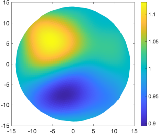
(a) Experiment 1 (ground truth)

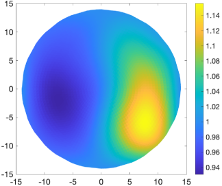
(b) Experiment 2 (ground truth)

Figure 1: Two randomly generated ground truth conductivity fields which were used to simulate the noisy electrode measurements for numerical inversion.

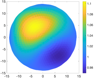
(a) Experiment 1 (reconstruction)

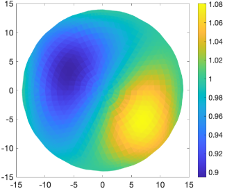
(b) Experiment 2 (reconstruction)

Figure 2: Reconstructions corresponding to noisy voltage measurements generated using the phantoms in Figure 1a and Figure 1b.

with

$$\psi_{j}({\boldsymbol{x}}):=\frac{5}{(k_{j}^{2}+\ell_{j}^{2})^{2}}\sin(\tfrac{1}{14}\pi k_{j}x_{1})\sin(\tfrac{1}{14}\pi\ell_{j}x_{2}),$$ (8)

where the sequence $(k_{j},\ell_{j})_{j\geq 1}$ is an ordering of the elements of $\mathbb{N}\times\mathbb{N}$ such that $\|\psi_{1}\|_{L^{\infty}(D)}\geq\|\psi_{2}\|_{L^{\infty}(D)}\geq\cdots$. We consider two different target conductivities which were obtained for two independent randomly generated vectors ${\boldsymbol{y}}\sim\mathcal{U}((-1/2,1/2)^{20})$. These target conductivities are illustrated in Figure 2. The voltage measurements were then simulated by solving the CEM forward model using a first order finite element discretization with maximum mesh diameter $h=0.748$. In addition, the measurements were contaminated with additive i.i.d. Gaussian noise with covariance $\Gamma=0.014I$. As the contact resistance of each electrode, we used the value $z_{k}=0.005$ for $k=1,\ldots,16$.

We approximate $\widehat{a}$ using the QMC ratio estimator with $n=2^{20}$ nodes. As the generating vector for the QMC rule, we used the “off-the-shelf” lattice generating vector [40, lattice-39101-1024-1048576.3600]. For the computational inversion, we used a coarser finite element mesh with mesh width $h=1.496$. The computational inversion used the same parametric model (7)–(8). The reconstructions for the two experiments are displayed in Figures 1a and 1b. In both cases, the profile and magnitude of the target conductivities are approximately recovered.

In addition, we also assessed the convergence of the QMC estimator. To this end, we computed the value of $\widehat{a}$ for $n=2^{\ell}$, $\ell=10,\ldots,20$, and report the approximated root-mean-square (R.M.S.) errors

$$\sqrt{\frac{1}{R(R-1)}\sum_{r^{\prime}=1}^{R}\bigg{(}\frac{1}{R}\sum_{r=1}^{R}\frac{Z_{n}^{\prime}(\boldsymbol{\delta},\boldsymbol{\Delta}^{(r)})}{Z_{n}(\boldsymbol{\delta},\boldsymbol{\Delta}^{(r)})}-\frac{Z_{n}^{\prime}(\boldsymbol{\delta},\boldsymbol{\Delta}^{(r^{\prime})})}{Z_{n}(\boldsymbol{\delta},\boldsymbol{\Delta}^{(r^{\prime})})}\bigg{)}^{2}}$$

in Figure 3 with $R=16$ random shifts $\boldsymbol{\Delta}^{(r)}\overset{\rm i.i.d.}{\sim}\mathcal{U}([0,1]^{20})$, $r=1,\ldots,16$. The convergence graphs display faster-than-Monte Carlo cubature convergence rates.

Figure 3: The R.M.S. errors for reconstructions corresponding to the reconstructions illustrated in Figures 1a and 1b with $R=16$ random shifts plotted alongside the corresponding least squares fits.

7 Conclusions

Many studies on the application of QMC methods to PDE uncertainty quantification problems focus on simplified PDE models with homogeneous boundary conditions. In this paper, we considered a more realistic PDE model with intricate mixed boundary conditions. Specifically, we were able to obtain parametric regularity bounds for both the forward model and the Bayesian inverse problem. Our numerical results illustrate that QMC integration results in more accurate estimation of the state with less computational work than using a Monte Carlo method. The quality of the reconstructed features can potentially be improved using more sophisticated prior models, e.g., involving basis functions with local supports, coupling the reconstruction method with importance sampling or Laplace approximation as well as employing optimal experimental design. In addition, in real-life measurement configurations there are unknown quantities other than the conductivity that need to be recovered such as the contact resistances, electrode positions, and the shape of the computational domain. These could also be included as part of the inference problem.

References

- [1] A. Chernov and T. Lê. Analytic and Gevrey class regularity for parametric elliptic eigenvalue problems and applications. SIAM J. Numer. Anal., 62(4):1874–1900, 2024.
- [2] A. D. Gilbert, I. G. Graham, F. Y. Kuo, R. Scheichl, and I. H. Sloan. Analysis of quasi-Monte Carlo methods for elliptic eigenvalue problems with stochastic coefficients. Numer. Math., 142(4):863–915, 2019.
- [3] P. A. Guth, V. Kaarnioja, F. Y. Kuo, C. Schillings, and I. H. Sloan. A quasi-Monte Carlo method for optimal control under uncertainty. SIAM/ASA J. Uncertain. Quantif., 9(2):354–383, 2021.
- [4] P. A. Guth, V. Kaarnioja, F. Y. Kuo, C. Schillings, and I. H. Sloan. Parabolic PDE-constrained optimal control under uncertainty with entropic risk measure using quasi-Monte Carlo integration. Numer. Math., 156:565–608, 2024.
- [5] A. Chernov and T. Lê. Analytic and Gevrey class regularity for parametric semilinear reaction-diffusion problems and applications in uncertainty quantification. Comput. Math. Appl., 164:116–130, 2024.
- [6] F. Y. Kuo and D. Nuyens. Application of quasi-Monte Carlo methods to elliptic PDEs with random diffusion coefficients: A survey of analysis and implementation. Found. Comput. Math., 16(6):1631–1696, 2016.
- [7] F. Y. Kuo, R. Scheichl, Ch. Schwab, I. H. Sloan, and E. Ullmann. Multilevel quasi-Monte Carlo methods for lognormal diffusion problems. Math. Comp., 86:2827–2860, 2017.
- [8] J. Dick, Q. T. Le Gia, and Ch. Schwab. Higher order quasi-Monte Carlo integration for holomorphic, parametric operator equations. SIAM/ASA J. Uncertain. Quantif., 4(1):48–79, 2016.
- [9] J. Dick, F. Y. Kuo, Q. T. Le Gia, D. Nuyens, and Ch. Schwab. Higher order QMC Petrov–Galerkin discretization for affine parametric operator equations with random field inputs. SIAM J. Numer. Anal., 52(6):2676–2702, 2014.
- [10] R. N. Gantner, L. Herrmann, and Ch. Schwab. Multilevel QMC with product weights for affine-parametric, elliptic PDEs. In J. Dick, F. Y. Kuo, and H. Woźniakowski, editors, Contemporary Computational Mathematics - A Celebration of the 80th Birthday of Ian Sloan, pages 373–405. Springer International Publishing, 2018.
- [11] I. G. Graham, F. Y. Kuo, J. A. Nichols, R. Scheichl, Ch. Schwab, and I. H. Sloan. Quasi-Monte Carlo finite element methods for elliptic PDEs with lognormal random coefficients. Numer. Math., 131(2):329–368, 2015.
- [12] I. G. Graham, F. Y. Kuo, D. Nuyens, R. Scheichl, and I. H. Sloan. Quasi-Monte Carlo methods for elliptic PDEs with random coefficients and applications. J. Comput. Phys., 230(10):3668–3694, 2011.
- [13] I. G. Graham, F. Y. Kuo, D. Nuyens, R. Scheichl, and I. H. Sloan. Circulant embedding with QMC: analysis for elliptic PDE with lognormal coefficients. Numer. Math., 140(2):479–511, 2018.
- [14] L. Herrmann and Ch. Schwab. QMC integration for lognormal-parametric, elliptic PDEs: local supports and product weights. Numer. Math., 141(1):63–102, 2019.
- [15] V. Kaarnioja, F. Y. Kuo, and I. H. Sloan. Uncertainty quantification using periodic random variables. SIAM J. Numer. Anal., 58(2):1068–1091, 2020.
- [16] F. Y. Kuo, Ch. Schwab, and I. H. Sloan. Quasi-Monte Carlo finite element methods for a class of elliptic partial differential equations with random coefficients. SIAM J. Numer. Anal., 50(6):3351–3374, 2012.
- [17] F. Y. Kuo, Ch. Schwab, and I. H. Sloan. Multi-level quasi-Monte Carlo finite element methods for a class of elliptic PDEs with random coefficients. Found. Comput. Math., 15(2):411–449, 2015.
- [18] J. Dick, R. N. Gantner, Q. T. Le Gia, and Ch. Schwab. Higher order quasi-Monte Carlo integration for Bayesian PDE inversion. Comput. Math. Appl., 77(1):144–172, 2019.
- [19] R. N. Gantner. Computational Higher-Order Quasi-Monte Carlo for Random Partial Differential Equations. PhD thesis, ETH Zurich, 2017.
- [20] R. N. Gantner and M. D. Peters. Higher-order quasi-Monte Carlo for Bayesian shape inversion. SIAM/ASA J. Uncertain. Quantif., 6(2):707–736, 2018.
- [21] L. Herrmann, M. Keller, and Ch. Schwab. Quasi-Monte Carlo Bayesian estimation under Besov priors in elliptic inverse problems. Math. Comp., 90:1831–1860, 2021.
- [22] R. Scheichl, A. M. Stuart, and A. L. Teckentrup. Quasi-Monte Carlo and multilevel Monte Carlo methods for computing posterior expectations in elliptic inverse problems. SIAM/ASA J. Uncertain. Quantif., 5(1):493–518, 2017.
- [23] C. Schillings, B. Sprungk, and P. Wacker. On the convergence of the Laplace approximation and noise-level-robustness of Laplace-based Monte Carlo methods for Bayesian inverse problems. Numer. Math., 145:915–971, 2020.
- [24] A. Adler and D. Holder. Electrical Impedance Tomography: Methods, History and Applications. Series in Medical Physics and Biomedical Engineering. CRC Press, 2021.
- [25] L. Borcea. Electrical impedance tomography. Inverse Problems, 18:R99–R136, 2002.
- [26] K.-S. Cheng, D. Isaacson, J. S. Newell, and D. Gisser. Electrode models for electric current computed tomography. IEEE Trans. Biomed. Eng., 36:918–924, 1989.
- [27] N. Hyvönen. Complete electrode model of electrical impedance tomography: approximation properties and characterization of inclusions. SIAM J. Appl. Math., 64(3):902–931, 2004.
- [28] E. Somersalo, M. Cheney, and D. Isaacson. Existence and uniqueness for electrode models for electric current computed tomography. SIAM J. Appl. Math., 52(4):1023–1040, 1992.
- [29] H. Harbrecht, M. Schmidlin, and Ch. Schwab. The Gevrey class implicit mapping theorem with application to UQ of semilinear elliptic PDEs. Math. Models Methods Appl. Sci., 34(05):881–917, 2024.
- [30] J. Dardé and S. Staboulis. Electrode modelling: the effect of contact impedance. ESAIM Math. Model. Numer. Anal., 50(2):415–431, 2016.
- [31] N. Hyvönen, V. Kaarnioja, L. Mustonen, and S. Staboulis. Polynomial collocation for handling an inaccurately known measurement configuration in electrical impedance tomography. SIAM J. Appl. Math., 77(1):202–223, 2017.
- [32] A. Cohen, R. DeVore, and Ch. Schwab. Convergence rates of best -term Galerkin approximations for a class of elliptic sPDEs. Found. Comput. Math., 10:615–646, 2010.
- [33] P. A. Guth and V. Kaarnioja. Quasi-Monte Carlo for partial differential equations with generalized Gaussian input uncertainty. Preprint 2024, arXiv:2411.03793 [math.NA].
- [34] R Dautray and J.-L. Lions. Mathematical Analysis and Numerical Methods for Science and Technology, volume 2. Springer-Verlag, Berlin, 1988.
- [35] V. Kaarnioja and C. Schillings. Quasi-Monte Carlo for Bayesian design of experiment problems governed by parametric PDEs. Preprint 2024, arXiv:2405.03529 [math.NA].
- [36] R. Cools, F. Y. Kuo, and D. Nuyens. Constructing embedded lattice rules for multivariate integration. SIAM J. Sci. Comput., 28:2162–2188, 2006.
- [37] J. Dick, F. Y. Kuo, and I. H. Sloan. High-dimensional integration: the quasi-Monte Carlo way. Acta Numer., 22:133–288, 2013.
- [38] D. Nuyens and R. Cools. Fast algorithms for component-by-component construction of rank-1 lattice rules in shift-invariant reproducing kernel hilbert spaces. Math. Comp., 75(254):903–920, 2006.
- [39] P. A. Guth and V. Kaarnioja. Generalized dimension truncation error analysis for high-dimensional numerical integration: lognormal setting and beyond. SIAM J. Numer. Anal., 62(2):872–892, 2024.
- [40] F. Y. Kuo. Lattice rule generating vectors. https://web.maths.unsw.edu.au/~fkuo/lattice/.