Optimal Control of 1D Semilinear Heat Equations with Moment-SOS Relaxations*

Abstract

We use moment-SOS (Sum Of Squares) relaxations to address the optimal control problem of the 1D heat equation perturbed with a nonlinear term. We extend the current framework of moment-based optimal control of PDEs to consider a quadratic cost on the control. We develop a new method to extract a nonlinear controller from approximate moments of the solution. The control law acts on the boundary of the domain and depends on the solution over the whole domain. Our method is validated numerically and compared to a linear-quadratic controller.

I INTRODUCTION

The control of nonlinear Partial Differential Equations (PDEs) presents additional challenges over the linear case, due to the inherent complexity and potential for chaotic behavior in these systems. Several contemporary problems in fluid dynamics [1], as well as in fluid-structure interaction ([2, 3]), require advanced control techniques to successfully drive the solution to the desired target state.

A first strategy to tackle that kind of problem is to consider linear control techniques such as the Linear-Quadratic Regulator (LQR). In the case of linear PDEs, it provides the optimal control law at the continuous level of the problem (see [4] for instance) which precedes any domain discretization, as well as in the finite-dimensional formulation that usually follows a PDE approximation scheme (e.g., Finite Difference/Element/Volume methods). One classic approach to extend the LQR to the class of nonlinear PDEs is to derive the controller from the linearized equation and apply it to the initial nonlinear problem [5]. This method requires the use of specific numerical techniques involving fine discretization of space and time [3]. However, LQR control laws are only efficient for initial states that are sufficiently close to the target. This implies that there exists a region of initial states in the solution space outside of which a LQR controller cannot drive the system towards the target. We illustrate this situation later in Section III-C.

More advanced methods consist in constructing nonlinear controllers for the control problem of nonlinear PDEs. In the literature, these methods can be divided into two main categories.

The first one gathers the approaches that construct a nonlinear control law from the continuous formulation of the model and then discretize the system. We shall denote these methods by "Model-Control-Discretize", see [6, Section 17.12]. Among these, the backstepping method [7] is particularly noteworthy for transforming the original system into a more manageable form for stabilization. It is based on control lyapunov functions [8] that ensure the stability of the target system. However, finding an appropriate control lyapunov function is often a difficult task because there is no systematic way to construct such functions, especially for strongly nonlinear systems. The process can be highly problem-specific and may require significant mathematical insight. Similarly, Koopman-based dynamic mode decomposition approaches (e.g., [9, 10]) use a specific change of variables, the Koopman transform, which converts the original nonlinear PDE into a linear PDE in a new set of variables. Again, the main challenge of the method relies in finding such a Koopman transform.

The second major category comprises the "Model-Discretize-Control" methods. Notable approaches within this family include methods based on Pontryagin’s maximum principle [11]. Other techniques solve the Hamilton-Jacobi-Bellman equation [12] or state-dependent Riccati equations [13] to derive a stabilizing control law. These approaches tackle high-dimensional problems and often require long computation time to converge. Recent advancements in machine learning control [14] provide a viable and innovative alternative to the methods discussed above.

We consider in this paper a moment-based approach that relies on the concept of occupation measures [15], which allows to relax the problem of control of nonlinear PDEs into a Linear Program (LP) in the space of Borel measures. The main interest of this framework is its overall convexity and its versatility, as it covers a wide variety of polynomial PDEs. The method falls into the category of "Model-Control-Discretize" approaches as it operates directly on the continuous formulation of the PDE control problem, thus avoiding the need for spatio-temporal discretization. However, this advantage comes at the expense of having to solve a sequence of convex semidefinite programming problems, or Linear Matrix Inequalities (LMI) of increasing size. This approach has already been applied to the 1D Burgers’ equation, first to extract a stabilizing distributed control [15], and later to derive the entropy solutions for Riemann problems [16, 17]. An SOS method dual to the moment method is followed in [18] and [19] to find lower bounds on integral variational problems. For optimal control of linear PDEs, [20] proposes to approximate measures on infinite-dimensional vector spaces with measures on finite-dimensional vector spaces. Measures supported on infinite-dimensional vector spaces are considered in [21] and are used to solve numerically the heat equation perturbed with a distributed quadratic nonlinearity.

The contributions of this article are threefold: First, we extend the framework of [15] to incorporate a quadratic cost on the control, similar to the LQR. Second, we develop a new method for reconstructing a boundary control in feedback form, based on the solution over the entire domain. Third, we validate our method on a practical case where we consider the boundary control problem of the 1D heat equation perturbed with linear and nonlinear terms. Fig. 1 outlines the main steps of our method of resolution. To the best of the authors’ knowledge, the problem of control of 1D semilinear heat equations has not yet been addressed using the moments of occupation measures supported on finite-dimensional spaces. It will serve as a possible starting point for further studies on harder, higher-dimensional control problems, such as 2D semilinear heat equations, fluid-structure interaction problems, etc.

Figure 1: Moment-based approach for the control of PDEs.

The remainder of this article is organized as follows. Section II presents the PDE control problem that we consider and our contribution to extend the framework of [15]. Section III discusses the validation of our method applied to a class of 1D semilinear heat equations. We demonstrate a case where the LQR approach derived from the linearized PDE cannot control the system towards the equilibrium, whereas the moment-based approach can. Finally, Section IV concludes the paper and outlines future research perspectives.

II Relaxation of PDE control problems into the space of occupation measures

II-A Problem statement

We denote by $\Omega=[0,1]\!\times\![0,1]$ the time-space domain, $\partial\Omega$ its boundary and $x=(x_{1},x_{2})\in\Omega$ the variables where $x_{1}$ typically represents the time and $x_{2}$ the position. We decompose the boundary of the domain into four parts $\partial\Omega=\partial\Omega_{I}\times\partial\Omega_{F}\times\partial\Omega_{W}\times\partial\Omega_{E}$. Fig. 2 illustrates this decomposition.

Figure 2: Definition of the domain and its boundaries. The red line indicates where the control is applied.

We consider the problem of control of the following 1D semilinear heat equation

$$\begin{dcases}\frac{\partial y}{\partial x_{1}}(x)=\lambda\frac{\partial^{2}y}{\partial x_{2}^{2}}(x)+\alpha y(x)+\eta y(x)^{3},\quad\forall x\in\Omega,\\ y(x)=0,\quad\forall x\in\partial\Omega_{W},\\ y(x)=u(x),\quad\forall x\in\partial\Omega_{E},\\ y(x)=y_{0}(x),\quad\forall x\in\partial\Omega_{I},\\ \end{dcases}$$ (1)

where $y\in W^{2,\infty}(\Omega)$ is the unknown scalar function, $u\in L^{2}(0,1)$ is the control, $y_{0}\in L^{2}(0,1)$ is a polynomial initial condition, $\lambda>0$ and $\alpha,\eta\geq 0$ are fixed parameters. We are interested in the problem of minimizing a functional $\mathcal{L}$ over the set of pairs $(y,u)$ subject to (1). We consider a quadratic cost function of the form

$$\mathcal{L}(y,u)=\frac{1}{2}\int_{\Omega}y(x)^{2}\,\mathrm{d}x+\frac{R}{2}\int_{0}^{1}u(x_{1})^{2}\,\mathrm{d}x_{1},$$ (2)

where $R>0$ is a fixed parameter. The optimal control problem of $\eqref{eq:heat1D}$ finally writes

$$\begin{array}[]{ll}\underset{\scriptstyle\text{$(y,u)\in W^{2,\infty}(\Omega)\times L^{2}(0,1),$}}{\inf}&\mathcal{L}(y,u),\\ \quad\quad\quad\,\,\,\,\,\,\text{s.t.}&\text{$(y,u)$ subject to \eqref{eq:heat1D}}.\end{array}$$ (3)

We denote by $\ell_{\inf}$ the infimum of (3).

II-B Occupation measures

We apply the nonlinear optimal control techniques developed in [15] to solve this problem. We consider $\textbf{Y}=\mathbb{R}$ such that $y$ lives in Y, $\textbf{Z}=\mathbb{R}^{2}$ such that $z=\nabla y$ lives in Z and $\textbf{U}=[u_{\mathrm{min}},u_{\mathrm{max}}]$ such that $u$ lives in U. We denote by $\mu$ the occupation measure associated to $y$ on $\Omega$ and $\mu_{I}$, $\mu_{F}$, $\mu_{W}$ and $\mu_{E}$ the boundary occupation measures associated to $y$ on $\partial\Omega_{I}$, $\partial\Omega_{F}$, $\partial\Omega_{W}$ and $\partial\Omega_{E}$, respectively. We modify the definition of the occupation measures given in [15] to include $u$ as a variable of $\mu_{E}$. This allows one to account for a quadratic cost on the control similar to the LQR approach.
Definition 1. The occupation measures are defined for all Borel sets $A\subset\Omega$, $A_{i}\subset\partial\Omega_{i}$ ($i\in\{I,F,W,E\}$), $B\subset\textbf{Y}$, $C\subset\textbf{Z}$ and $D\subset\textbf{U}$ by

$$\begin{split}&\mu(A\!\times\!B\!\times\!C)=\int_{\Omega}\mathds{1}_{A\times B\times C}(x,y(x),z(x))\,\mathrm{d}x,\\ &\mu_{i}(A_{i}\!\times\!B\!\times\!C)\!=\!\!\!\int_{\partial\Omega_{i}}\!\!\!\!\!\!\!\mathds{1}_{A_{i}\times B\times C}(x,y(x),z(x))\,\mathrm{d}\sigma(x),\ i\in\{I,F,W\},\\ &\mu_{E}(A_{E}\!\times\!B\!\times\!C\!\times\!D)\!=\!\!\!\int_{\partial\Omega_{E}}\!\!\!\!\!\!\!\mathds{1}_{A_{E}\times B\times C\times D}(x,y(x),z(x),u(x))\,\mathrm{d}\sigma(x),\end{split}$$

where $\sigma$ is the surface measure on $\partial\Omega$. We define $\Gamma=\Omega\times\textbf{Y}\times\textbf{Z}$, $\partial\Gamma_{E}=\partial\Omega_{E}\times\textbf{Y}\times\textbf{Z}\times\textbf{U}$ and for all $i\in\{I,F,W\}$, $\partial\Gamma_{i}=\partial\Omega_{i}\times\textbf{Y}\times\textbf{Z}$. The following proposition is an immediate consequence of Definition 1.
Proposition 1. For any bounded Borel measurable functions $h\,:\,\Gamma\rightarrow\mathbb{R}$ and $h_{i}\,:\,\partial\Gamma_{i}\rightarrow\mathbb{R}$ ($i\in\{I,F,W,E\}$), we have

$$\begin{split}&\int_{\Omega}h(x,y(x),z(x))\,\mathrm{d}x=\int_{\Gamma}h(x,y,z)\,\mathrm{d}\mu(x,y,z),\\ &\int_{\partial\Omega_{i}}\!\!\!\!h_{i}(x,y(x),z(x))\,\mathrm{d}x\!=\!\!\int_{\partial\Gamma_{i}}\!\!\!h_{i}(x,y,z)\,\mathrm{d}\mu_{i}(x,y,z),i\in\{I,F,W\},\\ &\int_{\partial\Omega_{E}}\!\!\!h_{E}(x,y(x),z(x),u(x))\,\mathrm{d}x\!=\!\!\int_{\partial\Gamma_{E}}\!\!\!h_{E}(x,y,z,u)\,\mathrm{d}\mu_{E}(x,y,z,u).\end{split}$$

One should note that on the right-hand side, $y$, $z$ and $u$ are no longer functions of $x$ but rather integrated variables.
We can deduce from Proposition 1 the weak formulation of (1) in terms of the occupation measures (see Theorem 1 in [15] for a detailed derivation). For all test functions $\phi\in C^{\infty}(\Omega\times\textbf{Y})$, we have

$$\begin{split}&\int_{\Gamma}\frac{\partial\phi}{\partial x_{1}}+z_{1}\frac{\partial\phi}{\partial y}\,\mathrm{d}\mu+\int_{\partial\Gamma_{I}}\phi\,\mathrm{d}\mu_{I}-\int_{\partial\Gamma_{F}}\phi\,\mathrm{d}\mu_{F}=0,\end{split}$$ (4a)

$$\begin{split}&\int_{\Gamma}\frac{\partial\phi}{\partial x_{2}}+z_{2}\frac{\partial\phi}{\partial y}\,\mathrm{d}\mu+\int_{\partial\Gamma_{W}}\phi\,\mathrm{d}\mu_{W}-\int_{\partial\Gamma_{E}}\phi\,\mathrm{d}\mu_{E}=0,\end{split}$$ (4b)

$$\begin{split}&\int_{\Gamma}\frac{\partial\phi}{\partial x_{1}}\!\left[z_{1}\!-\!\alpha y\!-\!\eta y^{3}\right]\!\,\mathrm{d}\mu\!-\!\!\!\int_{\Gamma}\left[\frac{\partial\phi}{\partial x_{2}}+z_{2}\frac{\partial\phi}{\partial y}\right]B_{2,2}z_{2}\,\mathrm{d}\mu\\ &\quad+\int_{\partial\Gamma_{E}}B_{2,2}\phi z_{2}\,\mathrm{d}\mu_{E}-\int_{\partial\Gamma_{W}}B_{2,2}\phi z_{2}\,\mathrm{d}\mu_{W}=0,\end{split}$$ (4c)

$$\begin{split}&\int_{\partial\Gamma_{I}}\phi\left[y-y_{0}(x)\right]\,\mathrm{d}\mu_{I}+\int_{\partial\Gamma_{E}}\phi\left[y-u\right]\,\mathrm{d}\mu_{E}\\ &\quad+\int_{\partial\Gamma_{W}}\phi y\,\mathrm{d}\mu_{W}=0,\end{split}$$ (4d)

where $\displaystyle z=[z_{1}\ z_{2}]^{T}$ and $B_{2,2}=-\lambda$. We omitted the dependency of the occupation measures with the variables of integration $x$, $y$, $z$ and $u$ in $\eqref{eq:weak_formulation_heat1D}$ for conciseness purpose. The weak formulation allows one to write an infinite-dimensional LP whose optimal value will provide a lower bound on the optimal value $\ell_{\inf}$ of (3). We denote by $\mathcal{M}(A)_{+}$ the set of all nonnegative Borel measures with supports included in the set $A$ and by $\mathcal{K}$ the convex cone $\displaystyle\mathcal{K}=\mathcal{M}(\Gamma)_{+}\times\mathcal{M}(\partial\Gamma_{I})_{+}\times\mathcal{M}(\partial\Gamma_{F})_{+}\times\mathcal{M}(\partial\Gamma_{W})_{+}\times\mathcal{M}(\partial\Gamma_{E})_{+}$. The infinite-dimensional LP thus writes

$$\begin{array}[]{ll}\!\!\!\!\!\!\!\underset{\left(\mu,\mu_{\partial_{I}},\ldots,\mu_{\partial_{E}}\right)\in\mathcal{K}}{\inf}\!\!\!\!\!&\displaystyle\frac{1}{2}\int_{\Gamma}y^{2}\,\mathrm{d}\mu+\frac{R}{2}\int_{\partial\Gamma_{E}}u^{2}\,\mathrm{d}\mu_{E}\\ \text{ subject to }&\eqref{eq:weak_stokes_1},\eqref{eq:weak_stokes_2},\eqref{eq:weak_domain},\eqref{eq:weak_boundary},\ \forall\phi\in C^{\infty}\!(\Omega\!\times\!\mathbf{Y}),\\ &\displaystyle\int_{\partial\Gamma_{i}}\psi(x)\,\mathrm{d}\mu_{i}=\int_{\partial\Omega_{i}}\psi(x)\,\mathrm{d}\sigma(x),\\ &\forall\psi\in C^{\infty}(\Omega),\ \forall i\in\{I,F,W,E\}.\end{array}$$ (5)

We denote by $\hat{\ell}_{\inf}$ the infimum of (5), which satisfies $\hat{\ell}_{\inf}\leq\ell_{\inf}$. Note that the LP formulation is a relaxation of the initial problem in the sense that the set of all measures $(\mu,\mu_{I},\ldots,\mu_{E})$ that satisfy the previous weak formulation may be strictly larger than the set of all occupation measures corresponding to the solution(s) of the PDE. The study of the existence of a relaxation gap for the general problem of optimal control of PDEs is still an open question with the most recent results in the nonconvex case being [22] and the convex case [23, 24].

In our case, the existence of a relaxation gap may only have a minor influence on our results, as our goal is not to solve (3) exactly, but rather to present a method for constructing a stabilizing nonlinear control law in a feedback form.

II-C LMI relaxations

In order to approximate the infimum $\hat{\ell}_{\inf}$ of (5), a hierarchy of finite-dimensional LMI relaxations is derived from the LP. The relaxation considers polynomial test functions of the form $\displaystyle\phi(x_{1},x_{2},y)=x_{1}^{\alpha_{1}}x_{2}^{\alpha_{2}}y^{\alpha_{3}}$ in the weak formulation and truncates up to a certain relaxation degree $\displaystyle d\geq\alpha_{1}+\alpha_{2}+\alpha_{3}$. We consider $\textbf{K}\in\{\Gamma,\partial\Gamma_{I},\partial\Gamma_{F},\partial\Gamma_{W},\partial\Gamma_{E}\}$ and we denote by $n_{\textbf{K}}$ the appropriate dimension such that $\textbf{K}\subset\mathbb{R}^{n_{\textbf{K}}}$. We construct a finite-dimensional outer approximation $\mathcal{M}_{d}(\textbf{K})_{+}$ of $\mathcal{M}(\textbf{K})_{+}$ that writes

$$\begin{split}\!\!\!\!\mathcal{M}_{d}(\textbf{K})_{+}=\Bigl{\{}\textbf{s}\in\mathbb{R}^{s_{n_{\textbf{K}}}(d)}\,\Big{|}\,&0\preceq M_{d}(\textbf{s}),\\ &0\preceq M_{d}(g_{i}^{(\textbf{K})},\textbf{s}),\,1\leq i\leq m_{\textbf{K}}\Bigr{\}},\end{split}$$ (6)

where $s_{n_{\textbf{K}}}(d)=\binom{n_{\textbf{K}}+d}{d}$ is the number of monomials of $n_{\textbf{K}}$ variables with degree less than or equal to $d$, $\preceq$ denotes positive semidefiniteness, $\{g_{i}^{(\textbf{K})},1\leq i\leq m_{\textbf{K}}\}$ are the polynomials that appear in the polynomial inequalities defining the semialgebraic set K, $M_{d}(\textbf{s})$ is the moment matrix of order $d$ and $M_{d}(g_{i}^{(\textbf{K})},\textbf{s})$ are the localizing matrices of order $d$ (for more details, see [25]). The convex cone $\mathcal{K}$ is therefore approximated by the convex semidefinite representable cone $\mathcal{K}_{d}=\mathcal{M}_{d}(\Gamma)_{+}\times\mathcal{M}_{d}(\partial\Gamma_{I})_{+}\times\mathcal{M}_{d}(\partial\Gamma_{F})_{+}\times\mathcal{M}_{d}(\partial\Gamma_{W})_{+}\times\mathcal{M}_{d}(\partial\Gamma_{E})_{+}$. The constraints of (5) can be rewritten as a linear equation of the form

$$A_{d}\textbf{s}=b_{d}$$

and the objective functional as a scalar product

$$c_{d}^{T}\textbf{s},$$

where $\displaystyle\textbf{s}=\left[\textbf{s}_{\mu}^{T}\enspace\textbf{s}_{\mu_{I}}^{T}\enspace\cdots\enspace\textbf{s}_{\mu_{E}}^{T}\right]^{T}$ is the truncated vector of moments of the occupation measures up to the degree $d$. The entries of $A_{d}$, $b_{d}$ and $c_{d}$ depend on the coefficients of the different polynomial expressions in the weak formulation. The Matlab toolbox GloptiPoly 3, [26], provides a well-suited framework that assembles automatically these entries. The degree $d$ finite-dimensional LMI relaxation of $\eqref{eq:LP_heat1D}$ finally writes

$$\begin{array}[]{ll}\underset{\textbf{s}\in\mathcal{K}_{d}}{\inf}&c_{d}^{T}\textbf{s}\\ \,\,\,\text{s.t.}&A_{d}\textbf{s}=b_{d}.\end{array}$$ (7)

We solve (7) with the MOSEK solver based on interior-point methods [27]. It provides a sequence $\displaystyle\left(\hat{\ell}_{\inf,d}^{\,\,\mathrm{SDP}}\right)_{d}$ of lower bounds of $\hat{\ell}_{\inf}$ that increases with the relaxation degree $d$. From the LMI relaxation, we also obtain pseudo-moments, which are approximations of the moments of the occupation measures.

II-D Extraction of a control law from the pseudo-moments

After solving the LMI problem, all the pseudo-moments up to the relaxation degree $d$ have been computed. We develop in this section a method to extract from the pseudo-moments a nonlinear feedback control law that depends on the solution over the whole domain. We suppose the following form of the control

$$u(x_{1})=\int_{0}^{1}\gamma(x_{1},x_{2},y(x_{1},x_{2}))\,\mathrm{d}x_{2},\quad\forall x_{1}\in[0,1],$$ (8)

where $\gamma$ is a multivariate polynomial of degree $m\in\mathbb{N}$. We denote by $\displaystyle\beta_{m}(x_{1},x_{2},y)=\left[1\enspace x_{1}\enspace x_{2}\enspace y\enspace x_{1}^{2}\enspace x_{1}x_{2}\enspace\cdots\enspace y^{m}\right]^{T}\in\mathbb{R}^{s_{3}(m)}$ the vector of all monomials up to degree $m$, sorted with the graded lexicographic ordering. There exists a vector of coefficients $c_{\gamma}\in\mathbb{R}^{s_{3}(m)}$ such that

$$\gamma(x_{1},x_{2},y)=\beta_{m}(x_{1},x_{2},y)^{T}c_{\gamma}.$$ (9)

We can multiply (8) by $\phi\in C^{\infty}([0,1])$, integrate in time and express the result in terms of the occupation measures. We obtain

$$\int_{\partial\Gamma_{E}}\phi(x_{1})u\,\mathrm{d}\mu_{E}=\left(\int_{\Gamma}\phi(x_{1})\beta_{m}(x_{1},x_{2},y)^{T}\,\mathrm{d}\mu\right)c_{\gamma},$$ (10)

where the integral on the right-hand side is taken component-wise. The test functions are chosen as $\phi(x_{1})=x_{1}^{k}$ for all $k\in\{0,\ldots,p\}$ and $p\in\mathbb{N}$, which leads to the resolution of a rectangular linear system

$$\Phi=Bc_{\gamma},$$ (11)

where $\Phi\in\mathbb{R}^{p+1}$ and $B\in\mathbb{R}^{(p+1)\times s_{3}(m)}$. We have for all $k\in\{1,\ldots,p+1\}$

$$\Phi_{k} =\int_{\partial\Gamma_{E}}x_{1}^{k-1}u\,\mathrm{d}\mu_{E},$$ (12a)

$$B_{k,\bullet} =\int_{\Gamma}x_{1}^{k-1}\beta_{m}(x_{1},x_{2},y)^{T}\,\mathrm{d}\mu,$$ (12b)

where $B_{k,\bullet}$ denotes the $k^{\mathrm{th}}$ row of the matrix $B$. Because the pseudo-moments have only been computed up to the relaxation degree $d$, (12a) and (12b) impose the condition $p\leq\min(d-1,d-m)$. If $p+1>s_{3}(m)$, the solution $c_{\gamma}^{*}$ to the system (11) is chosen to be the least-squares solution. Otherwise, $c_{\gamma}^{*}$ is chosen to be the minimum-norm solution for the Euclidean norm $\lVert\cdot\rVert_{2}$ in $\mathbb{R}^{s_{3}(m)}$. The choice of the norm is not inconsequential as it influences the coefficients of $\gamma$. We restrict our study to the Euclidean norm and leave the investigation of other norms for future work.

Note that (8) is not the only form of the control that can be recovered from the pseudo-moments. For instance, one could consider a control that is linear in the solution

$$u(x_{1})=\int_{0}^{1}y(x_{1},x_{2})\gamma_{\,\ell}(x_{1},x_{2})\,\mathrm{d}x_{2},$$ (13)

or semilinear as in

$$\!\!\!\!u(x_{1})\!=\!\int_{0}^{1}y(x_{1},x_{2})\gamma_{\,s\ell}(x_{1},x_{2})+y(x_{1},x_{2})^{r}\delta_{\,s\ell}(x_{1},x_{2})\,\mathrm{d}x_{2},$$ (14)

where $x_{1}\in[0,1]$, $r\geq 2$, $\gamma_{\,\ell}$ and $\gamma_{\,s\ell}$ are multivariate polynomials of degree $m$ and $\delta_{\,s\ell}$ is a multivariate polynomial of degree $m_{r}$. These control laws ultimately result in solving a rectangular linear system similar to (11). The key advantage of this reconstruction method is that it allows a wide range of controllers to be derived from the pseudo-moments, without the need for advanced numerical techniques beyond the resolution of (11).

III Numerical simulations

First, we assume that $\eta=0$ in (1). Notice that this case is the linearized version around the equilibrium state $y=0$ of (1) when $\eta\neq 0$. The resulting PDE is simply the heat equation, shifted by the linear term $\alpha y$. Note that the eigenvalues $\theta_{k}$ of the operator $\lambda\frac{\mathrm{d}^{2}}{\mathrm{d}x_{2}^{2}}+\alpha\operatorname{\mathbb{I}d}$ ($\operatorname{\mathbb{I}d}$ denotes the identity operator) with homogeneous Dirichlet boundary conditions are given by

$$\theta_{k}=\alpha-\lambda\pi^{2}k^{2},\quad\forall k\geq 1.$$ (15)

Thus, if $\alpha>\lambda\pi^{2}$, there is at least one positive eigenvalue and the solution of (1) naturally diverges if no control is applied.

We will first consider the LQR controller, which gives the theoretical optimal solution to the problem of Section II-A in the linear case, and compare it to linear and nonlinear controllers derived from the moment-based method.

III-A The linear-quadratic regulator

We use $P_{1}$-Lagrange finite elements on a uniform grid to approximate the solution of the PDE, which leads to the resolution of

$$\begin{dcases}M\dot{Y}(x_{1})=AY(x_{1})+BU(x_{1}),\quad\forall x_{1}>0,\\ Y(0)=Y_{0}\in\mathbb{R}^{N},\end{dcases}$$ (16)

where $Y\in\mathbb{R}^{N}$ approximates the solution $y(x_{1},\cdot)$ with $N$ degrees of freedom, $U\in\mathbb{R}$ approximates the control $u(x_{1})$ at $x_{2}=1$, and $M,A\in\mathbb{R}^{N\times N}$ and $B\in\mathbb{R}^{N}$ are the finite elements matrices and vector. The discrete cost function eventually reads

$$\!\!L(Y,U)=\frac{1}{2}\int_{0}^{\infty}Y(x_{1})^{T}QY(x_{1})\,\mathrm{d}x_{1}+\frac{R}{2}\int_{0}^{\infty}U(x_{1})^{2}\,\mathrm{d}x_{1},$$ (17)

where $R>0$ is the same as in (2) and $Q\in\mathbb{R}^{N\times N}$ is a positive semidefinite weight matrix on $Y$. The optimal pair minimizing $L$ is given by $\left(\bar{Y},\bar{U}\right)=\left(Y,-R^{-1}B^{T}PMY\right)$ where $P\in\mathbb{R}^{N\times N}$ is symmetric and solution to an Algebraic Riccati Equation (ARE) (see [28]).

The resolution of the ARE requires $N\left(N+1\right)/2$ unknown coefficients to be computed, hence the difficulties encountered when considering PDEs that require very fine meshing of the domain. In practice, the LQR is not derived on the full system but rather on a projection of the Riccati equation onto the unstable eigenspaces of the system (cf. [5]). Thus, for a small number $N_{u}$ of unstable components, the computational complexity can be significantly reduced. However, for large systems, the derivation of the spectrum is a numerical challenge on its own. Furthermore, the controller derived from this projection is subobtimal, as the optimal controller is given by the LQR derived on the full system.

Notice that unlike in (2), infinite-time integrals are considered in the discrete cost (17). This choice is justified by the results of the numerical simulations, as the infinite-time horizon LQR stabilizes the solution in short time (see Fig. 3). We could be more precise and solve a differential Riccati equation on the given finite-time horizon.

We present in Fig. 3 the results of the numerical simulations for the LQR. The parameters are fixed to $R=10^{-3}$, $\lambda=0.5$ and $\alpha=0.2+\lambda\pi^{2}$ such that exactly one unstable eigenvalue is forced. We choose a polynomial initial condition $\displaystyle y_{0}(x_{2})=10\,x_{2}^{2}\left(1-x_{2}\right)^{3}$ that satisfies the homogeneous Dirichlet boundary conditions. The solution of the PDE is computed using a backward differentiation scheme of order 2 with a time step $\Delta t=10^{-4}$. The space discretization uses $P_{1}$-Lagrange finite elements with a uniform mesh size $h=0.01$.

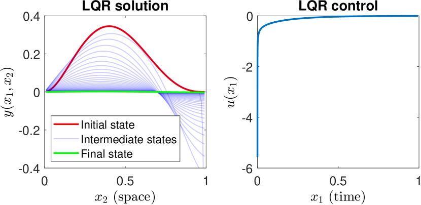
Figure 3: Numerical simulation of (1) with $\eta=0$ and the LQR controller.

Fig. 3 shows that the LQR successfully controls the solution to $y=0$. The variations of the controller are very steep around $x_{1}=0$ because the parameter $R$ is close to 0 and allows the norm of the control in (17) to be large. It acts as a regularization parameter, smoothing the control when increased. The optimal value $L^{*}$ of the discrete cost function is given by the LQR solution which, in this case, yields $L^{*}=L_{\mathrm{LQR}}\approx$1.829\text{\times}{10}^{-3}$$. In the following, every numerical result will be rounded to three decimal places.

III-B The linear case

In this section, we apply the moment-based method to our problem. The LMI problem is solved at the relaxation degree $d=6$ and we extract a linear controller of the form (13), where $\gamma_{\,\ell}$ is chosen to be constant, (i.e., $m=0$) and $p=d-1=5$. The least-squares solution of the linear system (11) in this case is given by the constant polynomial $\gamma_{\,\ell}(x_{1},x_{2})\approx-4.927$. We present the results of the numerical simulations in Fig. 4. We observe that the linear control derived from the pseudo-moments successfully controls the solution to 0.

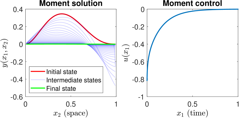
Figure 4: Numerical simulation of (1) with $\eta=0$ and a linear control extracted from the moments.

We can compare the value of the cost function for the pseudo-moment controller $L_{\mathrm{mom}}\approx$1.850\text{\times}{10}^{-3}$$ to the optimal value derived from the LQR controller. It corresponds to a relative error of $1.148$% from the optimal value $L_{\mathrm{LQR}}$. Thus, the linear controller extracted from the pseudo-moments is close to optimality and could be a promising alternative to the LQR. Indeed, in cases where the number of degrees freedom $N$ is too large to solve the Riccati equation, the moment-based method comes in handy as it does not rely on spatio-temporal gridding and can provide linear controllers similar to the LQR. This last remark is justified since the LQR can be expressed as a linear integral transform of the solution, where the kernel can be deduced from the adjoint state (see for instance [11, Chapter 3]). If the kernel is regular enough, (13) is a good approximation of the LQR.

III-C The nonlinear case

We now consider the semilinear PDE where $\eta\neq 0$. The purpose of this section is to demonstrate a scenario where the LQR controller, derived from the linearized equation with $\eta=0$ in Section III-A, fails to control the nonlinear PDE (1) towards the target state $y=0$. We present the results of the numerical simulations in Fig. 5. The parameters used for the simulation are identical to those used for Fig. 3, with $\eta$ set to $\eta=13\alpha$. The relaxation degree is $d=6$ and the control is computed from the pseudo-moments as a nonlinear feedback on the solution of the form (14), where $r=3$, $\gamma_{\,s\ell}$ is a polynomial of degree 1 and $\delta_{\,s\ell}$ is chosen to be constant. The resolution of the linear system (11) yields

$$\gamma_{\,s\ell}(x_{1},x_{2}) \approx-15.005+21.374\,x_{1}+1.231\,x_{2},$$ (18a)

$$\delta_{\,s\ell}(x_{1},x_{2}) \approx 3.369.$$ (18b)

We observe that the semilinear controller successfully steers the solution towards 0, while the LQR controller leads the solution to diverge. We stopped the simulation at the simulation time $T_{\mathrm{sim}}=0.9$ because when $t$ approaches 1, the pseudo-moment solution slowly moves away from the target state 0. Despite this behavior, we consider that this semilinear controller is satisfying enough as it drives the solution sufficiently close to 0 for standard linear control techniques to take over and maintain the solution near the target.

These results are promising because the method (cf. Fig. 1) can be readily applied to semilinear heat equations with polynomial nonlinear terms other than cubic. A trial and error type of search on the parameters $m$ and $p$ can be easily implemented to extract the nonlinear controller that gives the best results.

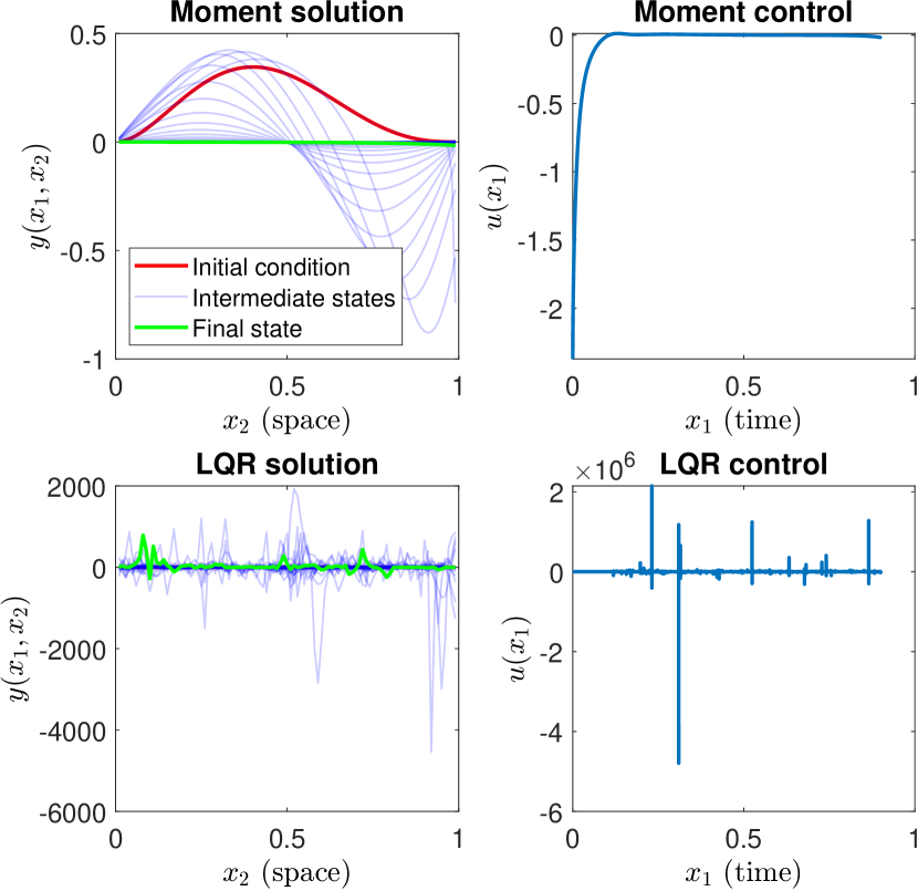
Figure 5: Numerical simulation of (1) with $\eta\neq 0$. Comparison of a nonlinear control law computed from the moments (top row) with the LQR controller (bottom row).

IV CONCLUSIONS

In this paper, an extended moment-SOS formulation, as well as an associated controller design method for a boundary optimal control problem of a 1D semilinear heat equation are presented. The proposed framework is an extension of that of [15] and allows one to consider a quadratic cost on the control. Additionally, a nonlinear feedback controller acting on the boundary of the domain is derived from pseudo-moments as the integral over the whole domain of a multivariate polynomial. The efficiency of our approach is demonstrated through numerical experiments in a case where traditional methods based on the linearized PDE fail because of the nonlinearity of the problem.

Future work will pursue several research directions including: (a) changing the polynomial basis in the moment-SOS hierarchy because the monomial basis is usually badly conditioned (e.g., the Chebyshev polynomial basis as in [29]); (b) exploiting the Christoffel-Darboux kernel to extract a control law from pseudo-moments (see for instance [30] for the reconstruction of the solution of a nonlinear PDE); (c) extending the method to 2D semilinear heat equations and, as a long term goal, to fluid-structure interaction control problems.

References

- [1] E. Bänsch, P. Benner, J. Saak, and H. K. Weichelt, “Riccati-based Boundary Feedback Stabilization of Incompressible Navier–Stokes Flows,” SIAM Journal on Scientific Computing, vol. 37, no. 2, pp. A832–A858, 2015.
- [2] A. Mini, C. Lerch, R. Wüchner, and K.-U. Bletzinger, “Computational closed-loop control of fluid-structure interaction (fsci) for lightweight structures,” PAMM, vol. 16, no. 1, pp. 15–18, 2016.
- [3] M. Fournié, M. Ndiaye, and J.-P. Raymond, “Feedback stabilization of a two-dimensional fluid-structure interaction system with mixed boundary conditions,” SIAM Journal on Control and Optimization, vol. 57, no. 5, pp. 3322–3359, 2019.
- [4] A. Bensoussan, G. Prato, M. C. Delfour, and S. K. Mitter, Eds., Representation and Control of Infinite Dimensional Systems, 2nd ed., ser. Systems & Control: Foundations & Applications. Boston, MA: Birkhäuser Boston, 2007.
- [5] C. Airiau, J.-M. Buchot, R. K. Dubey, M. Fournié, J.-P. Raymond, and J. Weller-Calvo, “Stabilization and Best Actuator Location for the Navier–Stokes Equations,” SIAM Journal on Scientific Computing, vol. 39, no. 5, pp. B993–B1020, 2017.
- [6] A. Quarteroni, Numerical Models for Differential Problems. Milano: Springer Milan, 2014.
- [7] M. Krstic and A. Smyshlyaev, Boundary Control of PDEs. Philadelphia, PA: Society for Industrial and Applied Mathematics, 2008.
- [8] J.-M. Coron, Control and Nonlinearity, ser. Mathematical Surveys and Monographs. Providence, Rhode Island: American Mathematical Society, 2009, vol. 136.
- [9] H. Arbabi, M. Korda, and I. Mezić, “A data-driven koopman model predictive control framework for nonlinear partial differential equations,” in 2018 IEEE Conference on Decision and Control (CDC), 2018, pp. 6409–6414.
- [10] S. Peitz and S. Klus, “Koopman operator-based model reduction for switched-system control of pdes,” Automatica, vol. 106, pp. 184–191, 2019.
- [11] F. Tröltzsch, Optimal control of partial differential equations: theory, methods, and applications, ser. Graduate studies in mathematics. Providence, R.I: American Mathematical Society, 2010, no. v. 112.
- [12] D. Kalise, S. Kundu, and K. Kunisch, “Robust feedback control of nonlinear pdes by numerical approximation of high-dimensional hamilton–jacobi–isaacs equations,” SIAM Journal on Applied Dynamical Systems, vol. 19, no. 2, pp. 1496–1524, 2020.
- [13] A. Alla, D. Kalise, and V. Simoncini, “State-dependent Riccati equation feedback stabilization for nonlinear PDEs,” Advances in Computational Mathematics, vol. 49, no. 1, p. 9, 2023.
- [14] T. Duriez, S. L. Brunton, and B. R. Noack, Machine Learning Control – Taming Nonlinear Dynamics and Turbulence, ser. Fluid Mechanics and Its Applications. Springer International Publishing, 2017, vol. 116.
- [15] M. Korda, D. Henrion, and J. B. Lasserre, “Moments and convex optimization for analysis and control of nonlinear pdes,” in Numerical Control: Part A, ser. Handbook of Numerical Analysis, E. Trélat and E. Zuazua, Eds. Elsevier, 2022, vol. 23, pp. 339–366.
- [16] S. Marx, T. Weisser, D. Henrion, and J. Lasserre, “A moment approach for entropy solutions to nonlinear hyperbolic PDEs,” 2018, arXiv:1807.02306.
- [17] C. Cardoen, S. Marx, A. Nouy, and N. Seguin, “A moment approach for entropy solutions of parameter-dependent hyperbolic conservation laws,” Numerische Mathematik, vol. 156, pp. 1–36, 2024.
- [18] G. Valmorbida, M. Ahmadi, and A. Papachristodoulou, “Stability analysis for a class of partial differential equations via semidefinite programming,” IEEE Transactions on Automatic Control, vol. 61, no. 6, pp. 1649–1654, 2016.
- [19] A. Chernyavsky, J. J. Bramburger, G. Fantuzzi, and D. Goluskin, “Convex relaxations of integral variational problems: Pointwise dual relaxation and sum-of-squares optimization,” SIAM Journal on Optimization, vol. 33, no. 2, pp. 481–512, 2023.
- [20] V. Magron and C. Prieur, “Optimal control of pdes using occupation measures and sdp relaxations,” IMA Journal of Mathematical Control and Information, 2017.
- [21] D. Henrion, M. Infusino, S. Kuhlmann, and V. Vinnikov, “Infinite-dimensional moment-SOS hierarchy for nonlinear partial differential equations,” arXiv e-prints, p. arXiv:2305.18768, 2023.
- [22] M. Korda and R. Rios-Zertuche, “The gap between a variational problem and its occupation measure relaxation,” arXiv preprint arXiv:2205.14132, 2022.
- [23] D. Henrion, M. Korda, M. Kruzik, and R. Rios-Zertuche, “Occupation measure relaxations in variational problems: the role of convexity,” SIAM Journal on Optimization, vol. 34, no. 2, pp. 1708–1731, 2024.
- [24] G. Fantuzzi and I. Tobasco, “Sharpness and non-sharpness of occupation measure bounds for integral variational problems,” arXiv preprint arXiv:2207.13570, 2022.
- [25] J. B. Lasserre, Moments, Positive Polynomials and Their Applications. Imperial College Press, 2009.
- [26] D. Henrion, J.-B. Lasserre, and J. Löfberg, “Gloptipoly 3: Moments, optimization and semidefinite programming,” Optimization Methods and Software, vol. 24, 2007.
- [27] M. Andersen, J. Dahl, Z. Liu, and L. Vandenberghe, “Interior-Point Methods for Large-Scale Cone Programming,” in Optimization for Machine Learning, S. Sra, S. Nowozin, and S. J. Wright, Eds. The MIT Press, 2011, pp. 55–84.
- [28] P. Lancaster and L. Rodman, Algebraic Riccati Equations. Oxford University Press, 1995.
- [29] D. Henrion, “Semidefinite characterisation of invariant measures for one-dimensional discrete dynamical systems,” Kybernetika, vol. 48, no. 6, pp. 1089–1099, 2012.
- [30] S. Marx, E. Pauwels, T. Weisser, et al., “Semi-algebraic approximation using christoffel–darboux kernel,” Constructive Approximation, vol. 54, pp. 391–429, 2021.