Learning a Neural Association Network for Self-supervised Multi-Object Tracking

Abstract

This paper introduces a novel framework to learn data association for multi-object tracking in a self-supervised manner. Fully-supervised learning methods are known to achieve excellent tracking performances, but acquiring identity-level annotations is tedious and time-consuming. Motivated by the fact that in real-world scenarios object motion can be usually represented by a Markov process, we present a novel expectation maximization (EM) algorithm that trains a neural network to associate detections for tracking, without requiring prior knowledge of their temporal correspondences. At the core of our method lies a neural Kalman filter, with an observation model conditioned on associations of detections parameterized by a neural network. Given a batch of frames as input, data associations between detections from adjacent frames are predicted by a neural network followed by a Sinkhorn normalization that determines the assignment probabilities of detections to states. Kalman smoothing is then used to obtain the marginal probability of observations given the inferred states, producing a training objective to maximize this marginal probability using gradient descent. The proposed framework is fully differentiable, allowing the underlying neural model to be trained end-to-end. We evaluate our approach on the challenging MOT17 and MOT20 datasets and achieve state-of-the-art results in comparison to self-supervised trackers using public detections. We furthermore demonstrate the capability of the learned model to generalize across datasets.

1 Introduction

Multi-object tracking (MOT) is highly relevant for many applications ranging from autonomous driving to understanding the behavior of animals. Thanks to the rapid development of object detection algorithms [14, 43, 50], tracking-by-detection has become the dominant paradigm for multi-object tracking. Given an input video, a set of detection hypotheses is first produced for each frame and the goal of tracking is to link these detection hypotheses across time, in order to generate plausible motion trajectories.

A large number of learning-based methods have focused on the fully-supervised MOT setting [21, 31, 8]. Specifically, these approaches assume that a training set with detections together with the associations between these detections are provided. Given this information, the goal is to train a model that can predict data association between detections during inference. While these approaches achieve strong performance on standard tracking benchmarks [39, 13], they demand costly labeling and annotation burdens that can be expensive to scale. In contrast to fully-supervised methods, self-supervised approaches seek to train a model that is able to temporally associate noisy detections, without requiring knowledge of the data association between them during training. Following this trend, Favyen et al. [2] recently designed a method that takes two modalities as input. While the first contains only bounding-box coordinates, the second contains appearance information solely. During training, the two inputs are forced to output the same association results. Similarly, Lu et al. [35] suggest to drop several detections within a track and utilize a path consistency constraint to train a network for association. This method achieves state-of-the-art performance in the self-supervised setting, but requires a number of heuristics and involves a complex removal strategy for training, which makes the training very expensive.

In this work, we introduce a novel framework to learn data association in a self-supervised manner. Motivated by the fact that object motion can be usually represented by a smooth Markov process, we propose an Expectation Maximization (EM) algorithm that finds associations, which rewards locally smooth trajectories over non-smooth associations. The core of our method relies on a neural Kalman filter [29, 27] and a differentiable assignment mechanism. The Kalman filter provides a principled way to model uncertainty in an efficient way since densities are evaluated in closed form. In particular, our Kalman filter’s motion model is realized by a random walk process while the observation model is parameterized by a neural network that provides the assignment probabilities of the observations to states via a permutation matrix. Since the permutation matrix should be doubly-stochastic, we propose to add a Sinkhorn layer into the system. Kalman smoothing [42] is then used to obtain the marginal probability of observations given inferred state trajectories, leading to a training objective that maximizes this marginal. As the Sinkhorn iterations merely involves normalization across rows and columns for several steps, the entire procedure is fully differentiable, allowing the underlying neural model to be trained in an end-to-end manner using gradient descent.

We further show how this approach can be used to successfully fine-tune an appearance model on the MOT17 [39] training set using association results produced by the trained association model, such that it enables better association abilities. During testing, we follow an online Kalman filter tracking paradigm [48] where the detections within the current frame are matched to the predicted detections from the previous frame using the learned association model.

In comparison to prior works [2, 35], our approach provides a principled and probabilistic way for self-supervised learning. The model can be trained in just a few minutes, which is much faster than [2, 35] which require about 24 hours for training. We evaluate our approach on the MOT17 and MOT20 [39, 13] datasets and show that our approach achieves better or comparable results than existing self-supervised multi-object tracking approaches. Furthermore, we demonstrate that the learned model generalizes across datasets. Our contributions are summarized as follows:

• We propose a novel self-supervised framework that embraces the Expectation Maximization algorithm to learn data association for MOT.

• The framework enables us to learn motion as well as appearance affinity together for robust data association and the learned association network naturally fits into the online tracking paradigm.

• Our approach achieves state-of-the-art performance among existing self-supervised MOT methods on the challenging MOT17 and MOT20 datasets with public detections.

2 Related Work

2.1 Self-Supervised Learning

Self-supervised learning usually defines a pretext task to generate pseudo labels, which can then be used to learn visual representations that can be applied in downstream vision tasks, eliminating the need to access expensive annotated labels as supervision. For example, Noroozi [40] learn useful representations by training a Siamese Convolutional Neural Network to solve a jigsaw puzzle. Larsson [30] formulates image colorization as a pretext task to learn useful visual representations. A further line of work [41, 9, 17] relies on the contrastive learning framework, where the idea is to model the similarity or dissimilarity of image pairs between two or multiple views, with or without having to define negative examples. An interesting work proposed by Asano et al. [1] even combines representation learning and clustering together. In their work, a fast version of the Sinkhorn-Knopp algorithm is used to generate pseudo cluster assignments for images and their method can scale to millions of input images and thousands of labels, achieving strong results. Caron et al. [7] propose a simple self-distillation training strategy for a Vision Transformer (ViT) architecture and show excellent performance for image segmentation. More recently, He [18] successfully trained an autoencoder network with the objective to reconstruct several randomly masked patches of a given image. The features learned by this approach demonstrate encouraging results on various downstream vision tasks. These works aim to learn general visual representations, but in the MOT context we require representations that specifically enable data association.

2.2 Self-Supervised Multi-Object Tracking

In the context of multi-object tracking, self-supervised MOT has the advantage that the training of data association models does not require expensive bounding box and track supervision, compared to its fully-supervised counterpart. SORT [5] adopts a simple Intersection-over-Union (IoU) as an affinity metric for data association. This approach, however, is sensitive to occlusions. Karthik et al. [24] utilize SORT [5] to generate pseudo track labels for training an appearance model which is then used in an online tracking framework. Jabbri et al. [23] propose to use cycle-consistency as a loss to learn an affinity measure for objects. The approach that works well in tracking multiple instance masks and human poses. Ho et al. [20] present a two-stage training strategy. It learns an appearance model for objects using an auto-encoder and represents MOT as a graph partitioning problem, which is solved by multi-cut clustering. This approach, however, does not scale and is slow during inference. Favyen et al. [2] propose a heuristic input masking strategy that enforces mutual consistency between two given input modalities as an objective during training, an approach that achieves strong results for data association. Lin et al. [32] presents a dynamical recurrent variational autoencoder architecture, but this approach requires pre-training of motion models whilst the data association between states and observations admits a simple closed-form solution, but it can only track fixed number of objects. Liu et al. [33] suggest to incorporate uncertainty into unsupervised training and their method achieves promising results. In contrast to these works, our approach provides a principled objective and it requires only minutes to train.

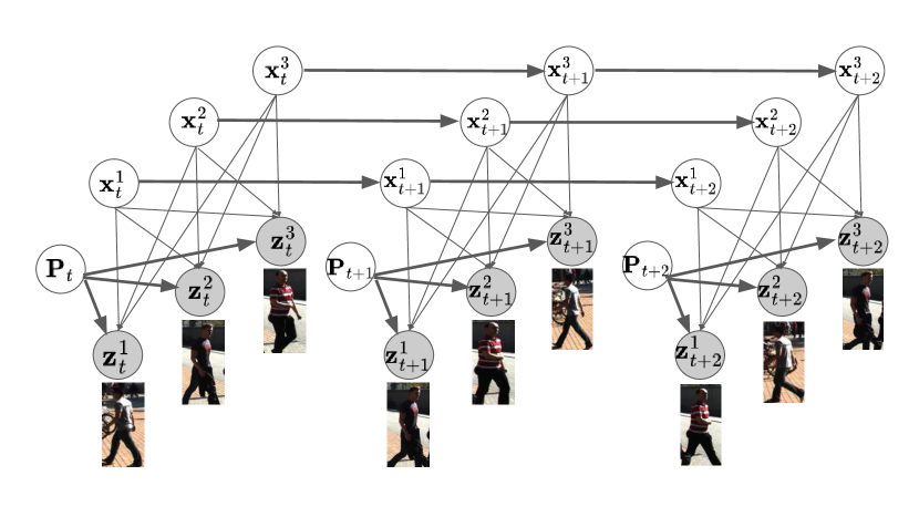
Figure 1: Given observations $\mathbf{z}_{1:T}$, a neural network is trained to predict the permutations $\mathbf{P}_{1:T}$ that assigns observations to states $\mathbf{x}_{1:T}$. The trained network can be used during inference to associate detections.

3 Neural Data Association using Expectation Maximisation

In this work, we propose a self-supervised learning approach for multi-object tracking. This means that only a set of unlabeled detections in a batch of frames are given and the goal is to train a neural network such that it can predict the associations of these detections accurately.

We rephrase this problem as a Kalman filtering problem as shown in Fig. 1. The unknown states of $K$ objects at the $t$-th time step are represented as $\mathbf{x}_{t}\in\mathbb{R}^{K\times d}$. Each object is represented by its $d$-dimensional state vector, containing its $x,y$ central coordinates as well as its velocity in the image plane, i.e. $\mathbf{x}=(x,y,\dot{x},\dot{y})$. The track of an object $k$ over $T$ frames is thus indicated by $\mathbf{x}^{k}_{1:T}$. $\mathbf{z}_{t}\in\mathbb{R}^{K\times d^{\prime}}$ represents the observed detections where each detection at frame $t$ is represented by a $d^{\prime}$-dimensional observation vector, containing bounding box coordinates and appearance features. In contrast to a classical Kalman filtering problem, we do not know to which state $\mathbf{x}^{k}_{t}$ an observation $\mathbf{z}^{l}_{t}$ belongs to. This association is modeled by a permutation matrix $\mathbf{P}_{t}$ which assigns the observations $\mathbf{z}_{t}$ to the states $\mathbf{x}_{t}$. For training, we assume that all $K$ objects are visible in all $T$ frames and we will discuss occlusions or false positive detections later.

Given $\mathbf{P}_{t}$, we can update the states using a linear Kalman filter [29] with Gaussian noise:

$$p(\mathbf{x}_{t}|\mathbf{x}_{t-1}) =\mathcal{N}(\mathbf{x}_{t};\mathbf{Fx}_{t-1},\mathbf{Q}_{t}),$$ (1)

$$p(\mathbf{z}_{t}|\mathbf{x}_{t},\mathbf{P}_{t}) =\mathcal{N}(\mathbf{z}_{t};\mathbf{H}_{t}\mathbf{P}_{t}\mathbf{x}_{t},\mathbf{R}_{t}),$$ (2)

where $\mathbf{Q}_{t}$ and $\mathbf{R}_{t}$ are Gaussian noise, $\mathbf{H}_{t}$ is the linear mapping from state space to observation space, and $\mathbf{x}_{t}=\mathbf{Fx}_{t-1}$ is the motion model. While we use a linear model, the approach can be extended to non-linear models or a learned dynamic model. $\mathbf{P}_{t}$ will be estimated by a neural network $g_{\theta}$ and we will learn the parameters of the network using expectation maximisation and back propagation.

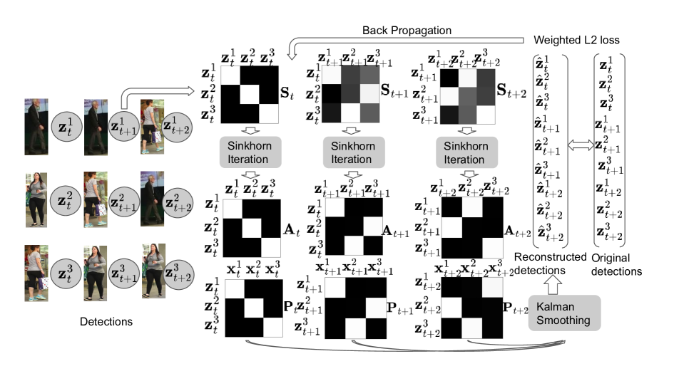
Figure 2: The proposed self-supervised learning framework. Given unlabeled detections $\mathbf{z}_{t:t+2}$, we train a neural network $g_{\theta}$ that predicts the score matrices $\mathbf{S}_{t:t+2}$ between detections from every pair of adjacent frames and for the first frame between all detections $\mathbf{z}_{t}$ of the same frame. For $\mathbf{S}_{t}$, the values should be thus high on the diagonal but low everywhere else. Sinkhorn normalization is then applied to $\mathbf{S}_{t:t+2}$ to produce the doubly stochastic association matrix $\mathbf{A}_{t:t+2}$, which associates detections between frames. The permutation matrices $\mathbf{P}_{t:t+2}$ then assign the detections to the states $\mathbf{x}$, where the state $\mathbf{x}^{k}_{t:t+2}$ represents a track of an object $k$. Kalman smoothing combined with the predicted $\mathbf{P}_{t:t+2}$ then reconstructs the detections, which are compared with original detections to define the loss in Eq. 8. This loss is then back-propagated to update the parameters of the network $g_{\theta}$. We only show three frames for simplicity, but the framework works on longer sequences.

3.1 Maximum Likelihood Learning Framework

Given the linear Gaussian motion and observation models (Eqs. 1 and 2), we can compute a predictive posterior, represented by state’s mean $\hat{\boldsymbol{\mu}}_{t}$ and covariance $\hat{\mathbf{\Sigma}}_{t}$ at timestep $t$, in closed form using a Kalman filter prediction step conditioned on a series of permutations $\mathbf{P}_{1:t-1}$:

$$= \mathcal{N}(\mathbf{x}_{t};\mathbf{F}\boldsymbol{\mu}_{t-1},\mathbf{F}\mathbf{\Sigma}_{t-1}\mathbf{F}^{T}+\mathbf{Q}_{t})$$

$$= \mathcal{N}(\mathbf{x}_{t};\hat{\boldsymbol{\mu}}_{t},\hat{\mathbf{\Sigma}}_{t})\,.$$ (3)

Here, $p(\mathbf{x}_{t-1}|\mathbf{z}_{1:t-1},\mathbf{P}_{1:t-1})$ is the Gaussian posterior at time $t-1$ from the last Kalman filter update step. Once the observations $\mathbf{z}_{t}$ are available at current timestamp $t$, the update equation for the posterior is given by:

$$p(\mathbf{x}_{t}|\mathbf{z}_{1:t},\mathbf{P}_{1:t})= \frac{p(\mathbf{z}_{t}|\mathbf{x}_{t},\mathbf{P}_{t})p(\mathbf{x}_{t}|\mathbf{z}_{1:t-1}\mathbf{P}_{1:t-1})}{p(\mathbf{z}_{t}|\mathbf{z}_{1:t-1}\mathbf{P}_{1:t})}$$ (4)

$$= \mathcal{N}(\mathbf{x}_{t};\boldsymbol{\mu}_{t},\mathbf{\Sigma}_{t})$$

$$\scalebox{0.85}{\mbox{$\displaystyle p(\mathbf{z}_{t}|\mathbf{z}_{1:t-1},\mathbf{P}_{1:t})$}}= \int p(\mathbf{z}_{t}|\mathbf{x}_{t},\mathbf{P}_{t})p(\mathbf{x}_{t}|\mathbf{z}_{1:t-1},\mathbf{P}_{1:t-1})d\mathbf{x}_{t}$$

The derivation above uses a Kalman filter that makes predictions based on a history of observations. During training, we use Kalman smoothing [42] to calculate the marginal as in Eq. 6, where $\tilde{\boldsymbol{\mu}}_{t}$ and $\tilde{\mathbf{\Sigma}}_{t}$ denote the smoothed mean and covariance of the current state $\mathbf{x}_{t}$, respectively:

$$p(\mathbf{z}_{t}|\mathbf{z}_{1:T},\mathbf{P}_{1:T})= \int p(\mathbf{z}_{t},\mathbf{x}_{t}|\mathbf{z}_{1:T},\mathbf{P}_{1:T})d\mathbf{x}_{t}$$ (6)

$$= \int p(\mathbf{z}_{t}|\mathbf{x}_{t},\mathbf{z}_{1:T},\mathbf{P}_{1:T})p(\mathbf{x}_{t}|\mathbf{z}_{1:T},\mathbf{P}_{1:T})d\mathbf{x}_{t}$$

$$= \int\mathcal{N}(\mathbf{z}_{t};\mathbf{H}_{t}\mathbf{P}_{t}\mathbf{x}_{t},\mathbf{R}_{t})\mathcal{N}(\mathbf{x}_{t};\tilde{\boldsymbol{\mu}}_{t},\tilde{\mathbf{\Sigma}}_{t})d\mathbf{x}_{t}$$

$$= \scalebox{0.9}{\mbox{$\displaystyle\mathcal{N}(\mathbf{z}_{t};\mathbf{H}_{t}\mathbf{P}_{t}\tilde{\boldsymbol{\mu}}_{t},(\mathbf{H}_{t}\mathbf{P}_{t})\tilde{\mathbf{\Sigma}}_{t}(\mathbf{H}_{t}\mathbf{P}_{t})^{T}+\mathbf{R}_{t})$}}.$$

This uses both a forward and backward process to condition on all observations $\mathbf{z}_{1:T}$, rather than conditioning only on prior observations at a given time step $\mathbf{z}_{1:t}$. It not only reduces uncertainty but also helps to ensure forward and backward temporal consistency in the associations of $\mathbf{z}_{1:T}$, providing more robust training.

Estimating $\mathbf{P}_{1:T}$. We delineate the detailed implementation pipeline in Fig. 2. Given detections $\mathbf{z}_{t-1}^{i}$ and $\mathbf{z}_{t}^{j}$ from frame $t-1$ and $t$, respectively, a network predicts their similarity $s_{ij}=g_{\theta}(\mathbf{z}_{t-1}^{i},\mathbf{z}_{t}^{j})$, with a higher value of $s_{ij}$ indicating higher similarity. By iterating over all detection pairs, we obtain a score matrix $\mathbf{S}_{t}$. From the score matrix, the Sinkhorn layer computes the association matrix $\mathbf{A}_{t}$ that associates detections between adjacent frames. As the permutation matrix $\mathbf{P}_{t}$ is required for training, we initialize the states in the first frame using the observations from the first frame, i.e., $\mathbf{x}_{1}=\mathbf{z}_{1}$, making $\mathbf{A}_{1}$ as the identity matrix. $\mathbf{P}_{t}$ is then obtained by $\mathbf{P}_{t}=\prod_{i=t}^{1}\mathbf{A}_{i}$.

Sinkhorn Layer. In general, the permutation $\mathbf{P}$ is a hard assignment matrix that makes it non-trivial to back-propagate the loss through it. It is therefore desirable to make it a “soft” version to enable gradient-based end-to-end training. The permutation matrix $\mathbf{P}$, however, needs to be doubly stochastic, i.e., its rows and columns should sum to one. To address this, we propose to add a Sinkhorn layer [46, 37] to normalize the score matrix $\mathbf{S}$:

$$\begin{split}X^{0}(\mathbf{S})=&\exp(\mathbf{S})\\ X^{l}(\mathbf{S})=&\mathcal{T}_{col}(\mathcal{T}_{row}(X^{l-1}(\mathbf{S})))\\ \mathbf{A}=&\lim_{l\rightarrow\infty}X^{l}(\mathbf{S})\end{split}$$ (7)

It applies the Sinkhorn operator [46] $X$ to the square matrix $\mathbf{S}$. In particular, $\mathcal{T}_{row}(\mathord{\cdot})$ and $\mathcal{T}_{col}(\mathord{\cdot})$ indicate row-wise and column-wise normalization operations, respectively. Repeating this for several iterations creates a doubly stochastic data association matrix $\mathbf{A}$ between detections. By combining Eq. 6 and $\mathbf{P}_{1:T}$, which depends on $\mathbf{S}_{1:T}$ and thus $g_{\theta}$, we define our training objective for $\theta$, which is optimized by gradient descent:

$$\scalebox{0.85}{\mbox{$\displaystyle\mathop{\arg\min}_{\theta}-\sum_{t=1}^{T}\log\mathcal{N}(\mathbf{z}_{t};\mathbf{H}_{t}\mathbf{P}_{t}\tilde{\boldsymbol{\mu}}_{t},(\mathbf{H}_{t}\mathbf{P}_{t})\tilde{\mathbf{\Sigma}}_{t}(\mathbf{H}_{t}\mathbf{P}_{t})^{T}+\mathbf{R}_{t})$}}.$$ (8)

The detailed training algorithm is shown in Algorithm 1. Intuitively this can be seen as an expectation maximisation (EM) approach that alternates between inferring underlying state trajectories, and identifying permutations mapping observations to trajectories.

Algorithm 1 The proposed procedure for learning data association.

Input: Observations $\mathbf{z}_{1:T}$, learning rate $\alpha$
  Output: $g_{\theta}(\mathord{\cdot})$

1:Initialize $\mathbf{A}_{1}$ using identical matrix, MLP with $\mathbf{\theta}_{0}$

2:for $n=1$ to number of iterations $N$ do

3:     for $t=2$ to $T$ do

4:         $\mathbf{S}_{t}=g_{\theta}(\mathbf{z}_{t-1},\mathbf{z}_{t})$

5:         Predict $\mathbf{A}_{t}$ using Sinkhorn iteration (Eq. 7)

6:         $\mathbf{P}_{t}=\prod_{i=t}^{1}\mathbf{A}_{i}$

7:         Compute $p(\mathbf{x}_{t}|\mathbf{z}_{1:t-1},\mathbf{P}_{1:t-1})$ using Sec. 3.1

8:         Compute $p(\mathbf{x}_{t}|\mathbf{z}_{1:t},\mathbf{P}_{1:t})$ using Eq. 4      

9:     for $t=T$ to $1$ do

10:         Compute $p(\mathbf{z}_{t}|\mathbf{z}_{1:T},\mathbf{P}_{1:T})$ using Eq. 6      

11:     Compute $\mathcal{L}{=}-\sum_{t=1}^{T}\log p(\mathbf{z}_{t}|\mathbf{z}_{1:T},\mathbf{P}_{1:T})$

12:     $\mathbf{\theta}_{n+1}=\mathbf{\theta}_{n}-\alpha\frac{\partial\mathcal{L}}{\partial\mathbf{\theta}}$

Return Learned MLP $g_{\theta_{N}}(\mathord{\cdot})$

Learning the Appearance Model. The aforementioned procedure only involves learning association between detections from adjacent frames using relative geometrical features. However, it is also desirable to learn an appearance model in order to associate objects when geometrical information is unreliable due to abrupt camera motion. To this end, we use the inferred associations from the previous step to train an appearance model $\phi_{\theta}(\mathord{\cdot})$.

Given a training sample that contains $K\times T$ detections, we first calculate the permutation matrix $\mathbf{P}_{T}\in\mathbb{R}^{K\times K}$, such that the rows indicate detections at the $T$-th frame and the columns denote detections at the first frame. Each element $p_{ij}$ represents the probability that detection $i$ at frame $T$ is associated to the detection $j$ at frame 1. We also construct a similarity matrix $\mathbf{U}_{T}\in\mathbb{R}^{K\times K}$ using the cosine similarity of appearance features, i.e., $u_{ij}=\phi_{\theta}(\mathbf{z}_{T}^{i})^{T}\phi_{\theta}(\mathbf{z}_{1}^{j})/||\phi_{\theta}(\mathbf{z}_{T}^{i})||^{2}||\phi_{\theta}(\mathbf{z}_{1}^{j}||^{2}$. The matrix $\mathbf{U}_{T}$ is normalized row-wise through softmax.

Intuitively, if the $i$-th detection at frame $T$ is associated with the $j$-th detection at the first frame, then their appearance similarity should also be high. Since $\mathbf{P}_{T}$ is a soft permutation matrix, we propose to minimize the KL-divergence between $\mathbf{P}_{T}$ and $\mathbf{U}_{T}$ as a second loss:

$$D_{KL}(\mathbf{P_{T}}||\mathbf{U_{T}})=\sum_{i}\sum_{j}p_{ij}\log\frac{p_{ij}}{u_{ij}}\,.$$ (9)

Minimizing this loss forces the appearance model to learn appearance features that agree with the learned associations. The rationale to choose appearance pairs that are temporally $T$ frames apart is to capture appearance changes over a longer period instead of incremental changes between two frames.

3.2 Inference

Combining Motion and Appearance Information. During inference, we define state $\mathbf{x}=(x,y,w,h,\dot{x},\dot{y},\dot{w},\dot{h})$, where $x,y,w,h$ denote bounding box’s central coordinates, width and height, $\dot{x},\dot{y},\dot{w},\dot{h}$ represent corresponding velocities. We use the learned networks $g_{\theta}$ and $\phi_{\theta}$ to associate objects within the Kalman filter framework. Suppose at frame $t$, we have $N$ bounding boxes $\hat{\mathbf{z}}_{t}$ predicted by the motion model along with $M$ detections $\mathbf{z}_{t}$, the cost matrix $\mathbf{C}\in\mathbb{R}^{N\times M}$ is used for association.

In our formulation, the observation contains both bounding box coordinates and motion information, as well as appearance information. This motivates us to combine both motion and appearance to define the cost to associate detections:

where $s_{\min}$ is the minimum cosine similarity threshold for two detections belonging to the same track and $\kappa$ is the scaling factor for the cosine similarity between two detections.

Detection Noise Handling. In practice, a predicted box at frame $t$ might not be matched to any detection due to occlusion or a missing detection. Vice versa, a detection at frame $t$ may not be matched to any of the predicted boxes as it could be a false positive or start of a new track. To handle this, we propose to further augment $\mathbf{C}$ with an auxiliary row and column containing a cost $c_{\text{miss}}$ for a missing association, such that $\mathbf{C}\in\mathbb{R}^{(N+1)\times(M+1)}$. We then obtain the optimal data association $\mathbf{A}^{\ast}$ by solving

$$\displaystyle\mathbf{A}^{\ast} =\mathop{\arg\min}_{\mathbf{A}\in\mathcal{A}}\sum_{i=1}^{N+1}\sum_{j=1}^{M+1}c_{ij}a_{ij},$$ (11)

s.t. $$\sum_{j=1}^{M+1}a_{ij}=1,\quad\forall i\in\{1,\cdots,N+1\},$$ (12)

$$\sum_{i=1}^{N+1}a_{ij}=1,\quad\forall j\in\{1,\cdots,M+1\}.$$ (13)

using the Hungarian algorithm [28]. In this way, tracks that are unmatched will only be updated by the motion model and detections that are unmatched to predictions initialize a new track if the detection confidence is high enough. We keep unmatched tracks for $\tau$ frames.

4 Experiments

4.1 Datasets

Our experiments are mainly conducted on the MOT17 and MOT20 datasets for pedestrian tracking. MOT17 contains 7 videos for training and 7 for testing. For all videos, detections from DPM [14], FRCNN [43] and SDP [50] are provided, resulting in 21 videos in total for training and testing. For MOT20, 4 videos are provided for training and testing under crowded scenarios. For evaluation, we report standard CLEAR [4] metrics such as MOTA and number of identity switches (IDS). We also report IDF1 and the HOTA metric [36].

4.2 Implementation Details

Preprocessing Detections. During training, we use Faster RCNN [43] detections. Our formulation attempts to track $K$ objects in a single clip, so we collect $K\times T$ detections from a single video clip, where $T$ is the clip length. While $K$ can differ for each clip, we keep $T$ the same for all clips. For the sake of computational efficiency, we generate the video clips with $T=10$ from each training sequence. Overall, we generate 260 videos from MOT17-02, MOT17-05, MOT17-09, MOT17-11 sequences for training.

We threshold the detections based on the detection confidence values to remove potential false positives. The number of remaining detections in the first frame of each clip defines $K$. To compensate for missing detections, we use the KCF [19] tracker, initialized independently for each detection at the first frame of the clip. In case there exist missing detections at certain frames, we use the bounding box output of the KCF for detection compensation. If this results in more than $K$ detections in the next frame, we discard detections with a low intersection-over-union with tracked bounding boxes.

During testing, we follow previous works [21, 2] and utilize Tracktor [3] to preprocess the provided raw detections, for online tracking as described in Sec. 3.2.

Features. Given a pair of detections $\mathbf{z}_{i}=(x_{i},y_{i},w_{i},h_{i})$ and $\mathbf{z}_{j}=(x_{j},y_{j},w_{j},h_{j})$, where $x$, $y$ is the bounding box’s central coordinate and $w$, $h$ being its width and height. The pairwise geometric feature is designed as:

These pairwise features serve as the input to $g_{\theta}(\mathord{\cdot})$ for regressing the score matrix $\mathbf{S}$. To extract appearance features, we resize each bounding box $\mathbf{z}$ to $128\times 64$ before feeding it to the appearance model $\phi_{\theta}(\mathord{\cdot})$ to obtain a 512 dimensional embedding $\phi_{\theta}(\mathbf{z})$, followed by L2 normalization.

Training Details. Our implementation is based on the PyTorch framework. We use the detections’ first frame coordinates to initialize state $\mathbf{x}_{1}$’s mean $\boldsymbol{\mu}_{1}$ and, the covariance matrix $\mathbf{\Sigma}_{1}$ is initialized as a diagonal matrix with variance set to 300. For the motion model $\mathbf{F}$ in the Kalman filter, a constant velocity model is utilized. The process noise $\sigma_{q}$ in the diagonal covariance matrix $\mathbf{Q}$ is set to 150 and the observation noise $\sigma_{r}$ within diagonal covariance matrix $\mathbf{R}$ is set to 5. This enables the Kalman filter to rely more on the observation model during training. We have also experimented with updating the parameters of $\mathbf{Q}$ during training but the differences were marginal as long as $\mathbf{Q}$ is initialized to a large value. The network $g_{\theta}(\mathord{\cdot})$ is implemented as two-layer MLP with ReLU non-linearity and the Sinkhorn normalization procedure takes 20 iterations. We optimize the parameters of $g_{\theta}(\mathord{\cdot})$ using the Adam [26] optimizer with learning rate of $10^{-2}$ for 10 epochs. We then proceed to fine-tune an ImageNet pretrained appearance model $\phi_{\theta}(\mathord{\cdot})$ using the OSNet [54] architecture, using Adam [26] with a learning rate of $10^{-4}$ for 3 epochs. Note that we only use the unlabeled detections from MOT17 training set to fine-tune the appearance models without additional training data.

4.3 Ablation Study

Impact of $\tau$. We study how the tracking performance is affected by the number of frames used for re-identification after occlusion. From Fig. 3, we observe a consistent gain among tracking metrics by increasing $\tau$, since the HOTA saturates around 60, we set $\tau=60$ in the final model.

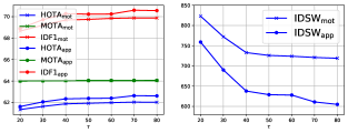
Figure 3: Tracking results influenced by different $\tau$.

Impact of adding Appearance Cost. In order to demonstrate the effectiveness of fine-tuning the appearance model, we conduct experiments on the MOT17 training set with public detections. As can be seen in Table 1, combining appearance cost can further boost the model’s tracking performance on all metrics. In particular, it reduces the number of identity switches (IDSW) by 13%.

Baseline Comparison. We compare our method to a strong baseline [24] that uses SORT to generate pseudo labels for learning an appearance model in Table 2. The approach adopts heuristics to define a similarity metric for generating labels. Our approach directly learns the appearance model together with the association of detections. Since [24] uses a better detector, i.e. CenterNet, to improve public detections, the MOTA is slightly higher for [24]. Nevertheless, our tracker outperforms [24] by 3.2 HOTA and 4.8 IDF1 and largely reduces IDS, showing the superiority of our method.

Association cost	HOTA $\uparrow$	MOTA $\uparrow$	IDF1 $\uparrow$	IDS $\downarrow$
mot	62.0	64.0	69.8	724
mot + app	62.4	64.1	70.2	628

Table 1: Ablations on the MOT17 training set using public detections.

Method	HOTA $\uparrow$	MOTA $\uparrow$	IDF1 $\uparrow$	IDS $\downarrow$
[24]	46.9	61.7	58.1	1864
Ours	50.1	60.2	62.9	1360

Table 2: Comparison with baseline approach on MOT17 test set using public detections.

4.4 Comparison with the State-of-the-Art

Finally, we evaluate our method on the MOT17 [39], MOT20 [13] and KITTI [16] benchmarks using the provided public detections and compare it to several other trackers. For MOT17, we also compare to other approaches using private detections although this does not provide a direct comparison since each method uses different detections.

Method	Sup.	HOTA $\uparrow$	MOTA $\uparrow$	IDF1 $\uparrow$	IDS $\downarrow$
MHT_BiLSTM [25]	✓	41.0	47.5	51.9	2069
Tracktor++ [3]	✓	44.8	56.3	55.1	1987
DeepMOT [49]	✓	-	53.7	53.8	1947
SUSHI [8]	✓	54.6	62.0	71.5	1041
SORT [5]	✗	-	43.1	39.8	4852
UNS20regress [2]	✗	46.4	56.8	58.3	1320
Lu et al. [35]	✗	49.0	58.8	61.2	1219
Ours	✗	50.1	60.2	62.9	1360

Table 3: Benchmark results on MOT17 test set using public detections, ✓indicates fully-supervised and ✗means self-supervised methods. The best and second best self-supervised performances are shown in bold and underlined numbers, respectively

Method	Sup.	HOTA $\uparrow$	MOTA $\uparrow$	IDF1 $\uparrow$	IDS $\downarrow$
MOTR [51]	✓	57.8	73.4	68.6	2439
MeMOTR [15]	✓	58.8	72.8	71.5	1902
MOTRv2 [53]	✓	62.0	78.6	75.0	2619
UCSL [38]	✗	58.4	73.0	70.4	-
OUTrack [34]	✗	58.7	73.5	70.2	4122
PointID [45]	✗	-	74.2	72.4	2748
ByteTrack [52]	✗	63.1	80.3	77.3	2196
U2MOT [33]	✗	64.2	79.9	78.2	1506
Lu et al. [35]	✗	65.0	80.9	79.6	1749
Ours	✗	63.1	80.4	78.0	1527

Table 4: Benchmark results on MOT17 test set using private detections, ✓indicates fully-supervised and ✗means self-supervised methods. The best and second best self-supervised performances are shown in bold and underlined numbers, respectively

Method	Sup.	HOTA $\uparrow$	MOTA $\uparrow$	IDF1 $\uparrow$	IDS $\downarrow$
Tracktor++V2 [3]	✓	42.1	52.6	52.7	1648
ArTist [44]	✓	-	53.6	51.0	1531
ApLift [22]	✓	46.6	58.9	56.5	2241
SUSHI [8]	✓	55.4	61.6	71.6	1053
SORT20 [5]	✗	36.1	42.7	45.1	4470
Ho et al. [20]	✗	-	41.8	-	5918
UnsupTrack [24]	✗	41.7	53.6	50.6	2178
Ours	✗	46.1	59.0	56.6	1832

Table 5: Benchmark results on MOT20 test set using public detections, ✓indicates fully-supervised and ✗means self-supervised methods. The best and second best self-supervised performances are shown in bold and underlined numbers, respectively

Method	Sup.	HOTA $\uparrow$	AssA $\uparrow$	DetA $\uparrow$	MOTA $\uparrow$
FAMNet [11]	✓	52.6	45.5	61.0	75.9
TuSimple [10]	✓	71.6	71.1	72.6	86.3
PermaTr [47]	✓	78.0	78.4	78.3	91.3
SORT [5]	✗	42.5	41.3	44.0	53.2
UNS20regress [2]	✗	62.5	65.3	61.1	-
OC_SORT [6]	✗	76.5	76.4	77.2	90.8
Lu et al. [35]	✗	78.8	80.3	77.9	91.0
Ours	✗	76.6	77.8	76.3	90.1

Table 6: Benchmark results on KITTI [16] test set for Car tracking. The best and second best self-supervised performances are shown in bold and underlined numbers, respectively. We use the same detections as used in OC-SORT

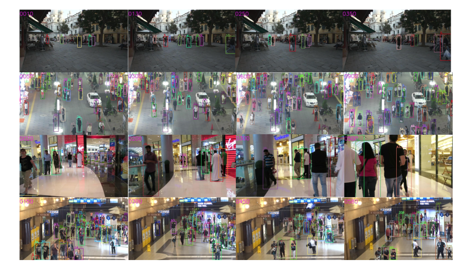
Figure 4: Qualitative results of our tracking method on MOT17/20 test set. Our method is able to track persons through long-term occlusions despite occlusion/camera motion/crowded scenarios, best viewed in color.

MOT17. We compare our method with several other approaches in Table 3. SORT [5] relies on IoU matching within a Kalman filter framework. Ho et al. [20] trains an appearance model using an auto-encoder network. Bastani’s work [2] utilizes motion and appearance consistency trained with an RNN for association. Lu et al. [35] impose a path consistency constraint with several loss terms to train a matching network, both [2] and [35] adopt heuristics as the training objective. Thanks to the principled maximum likelihood learning framework, our method outperforms all these approaches.

It is worth noting that the proposed tracker performs even better than several supervised approaches like MHT_BiLSTM [25], Tracktor++ [3] and DeepMOT [49], which either involve learning appearance models using identity-level annotations or designing differentiable frameworks for learning association costs.

We also compare our approach with other works under the private detection protocol in Table 4. Our tracker achieves results comparable with the state of the art [33, 35] and outperforms several transformer-based methods [51, 53, 15].

MOT20. Table 5 shows our results on MOT20. Our method outperforms SORT [5] and Ho et al. [20] by a large margin. It also surpasses UnsupTrack [24], which utilizes the tracklets produced by SORT [5] to fine-tune an appearance model, by a large margin in all tracking metrics. Our approach achieves state-of-the-art performance on this dataset.

KITTI. We evaluated the generalization of the learned model by evaluating the model, that has been trained on MOT17 for pedestrian tracking, on KITTI for car tracking. Since the appearance is different, we only utilize the motion cost for inference and we did not train a specific appearance model. The results are reported in Table 6. The learned motion cost generalizes well across the datasets. Our method achieves a slightly higher HOTA than the strong baseline OC-SORT [6]. While the state-of-the-art approach [35] performs better, it has been trained on the dataset. Given that we did not train our approach on KITTI, the reported results are impressive.

Qualitative Results. Fig. 4 shows some qualitative results for the MOT17 and MOT20 test set. Our method can track objects with similar appearances under occlusion, camera motion and crowded scenarios, despite learning data associations in a self-supervised manner. Thanks to the online inference procedure, our tracker can be readily applied in real-time applications, as opposed to approaches [21, 22, 12, 31] that work in an offline manner.

5 Conclusion

In summary, this work introduces a maximum likelihood learning framework for self-supervised multi-object tracking. It learns a network for associating detections between adjacent frames and an appearance model by associating detections to states of a Kalman filter. Our method does not require expensive identity-level annotations for training and the entire training requires only several minutes. Our approach enables online inference and achieves state-of-the-art performances on the challenging MOT17 and MOT20 datasets among existing self-supervised approaches with public detections. Furthermore, we have demonstrated that the learned network generalizes across datasets. While the results are promising, the approach has some limitations. For instance, we do not explicitly model the appearing and disappearing of objects during training. While this is not a major limitation since we only consider 10 frames and handle such cases during inference, such a handling could be a future extension. In the future, we also plan to study whether it is possible to learn object detectors as well as the association network jointly within this maximum likelihood learning framework.

References

- Asano et al. [2019] Yuki Markus Asano, Christian Rupprecht, and Andrea Vedaldi. Self-labelling via simultaneous clustering and representation learning. arXiv preprint arXiv:1911.05371, 2019.
- Bastani et al. [2021] Favyen Bastani, Songtao He, and Samuel Madden. Self-supervised multi-object tracking with cross-input consistency. Advances in Neural Information Processing Systems, 34:13695–13706, 2021.
- Bergmann et al. [2019] Philipp Bergmann, Tim Meinhardt, and Laura Leal-Taixe. Tracking without bells and whistles. In Proceedings of the IEEE/CVF International Conference on Computer Vision, pages 941–951, 2019.
- Bernardin and Stiefelhagen [2008] Keni Bernardin and Rainer Stiefelhagen. Evaluating multiple object tracking performance: the clear mot metrics. EURASIP Journal on Image and Video Processing, 2008:1–10, 2008.
- Bewley et al. [2016] Alex Bewley, Zongyuan Ge, Lionel Ott, Fabio Ramos, and Ben Upcroft. Simple online and realtime tracking. In 2016 IEEE international conference on image processing (ICIP), pages 3464–3468. IEEE, 2016.
- Cao et al. [2023] Jinkun Cao, Jiangmiao Pang, Xinshuo Weng, Rawal Khirodkar, and Kris Kitani. Observation-centric sort: Rethinking sort for robust multi-object tracking. In Proceedings of the IEEE/CVF conference on computer vision and pattern recognition, pages 9686–9696, 2023.
- Caron et al. [2021] Mathilde Caron, Hugo Touvron, Ishan Misra, Hervé Jégou, Julien Mairal, Piotr Bojanowski, and Armand Joulin. Emerging properties in self-supervised vision transformers. In Proceedings of the IEEE/CVF international conference on computer vision, pages 9650–9660, 2021.
- Cetintas et al. [2023] Orcun Cetintas, Guillem Brasó, and Laura Leal-Taixé. Unifying short and long-term tracking with graph hierarchies. In Proceedings of the IEEE/CVF Conference on Computer Vision and Pattern Recognition, pages 22877–22887, 2023.
- Chen et al. [2020] Ting Chen, Simon Kornblith, Mohammad Norouzi, and Geoffrey Hinton. A simple framework for contrastive learning of visual representations. In International conference on machine learning, pages 1597–1607. PMLR, 2020.
- Choi [2015] Wongun Choi. Near-online multi-target tracking with aggregated local flow descriptor. In Proceedings of the IEEE international conference on computer vision, pages 3029–3037, 2015.
- Chu and Ling [2019] Peng Chu and Haibin Ling. Famnet: Joint learning of feature, affinity and multi-dimensional assignment for online multiple object tracking. In Proceedings of the IEEE/CVF International Conference on Computer Vision, pages 6172–6181, 2019.
- Dai et al. [2021] Peng Dai, Renliang Weng, Wongun Choi, Changshui Zhang, Zhangping He, and Wei Ding. Learning a proposal classifier for multiple object tracking. In Proceedings of the IEEE/CVF Conference on Computer Vision and Pattern Recognition, pages 2443–2452, 2021.
- Dendorfer et al. [2019] P Dendorfer, H Rezatofighi, A Milan, J Shi, D Cremers, I Reid, S Roth, K Schindler, and L Leal-Taixe. Cvpr19 tracking and detection challenge: How crowded can it get? arxiv 2019. arXiv preprint arXiv:1906.04567, 2019.
- Felzenszwalb et al. [2009] Pedro F Felzenszwalb, Ross B Girshick, David McAllester, and Deva Ramanan. Object detection with discriminatively trained part-based models. IEEE transactions on pattern analysis and machine intelligence, 32(9):1627–1645, 2009.
- Gao and Wang [2023] Ruopeng Gao and Limin Wang. Memotr: Long-term memory-augmented transformer for multi-object tracking. In Proceedings of the IEEE/CVF International Conference on Computer Vision, pages 9901–9910, 2023.
- Geiger et al. [2012] Andreas Geiger, Philip Lenz, and Raquel Urtasun. Are we ready for autonomous driving? the kitti vision benchmark suite. In Conference on Computer Vision and Pattern Recognition (CVPR), 2012.
- He et al. [2020] Kaiming He, Haoqi Fan, Yuxin Wu, Saining Xie, and Ross Girshick. Momentum contrast for unsupervised visual representation learning. In Proceedings of the IEEE/CVF conference on computer vision and pattern recognition, pages 9729–9738, 2020.
- He et al. [2022] Kaiming He, Xinlei Chen, Saining Xie, Yanghao Li, Piotr Dollár, and Ross Girshick. Masked autoencoders are scalable vision learners. In Proceedings of the IEEE/CVF conference on computer vision and pattern recognition, pages 16000–16009, 2022.
- Henriques et al. [2014] João F Henriques, Rui Caseiro, Pedro Martins, and Jorge Batista. High-speed tracking with kernelized correlation filters. IEEE transactions on pattern analysis and machine intelligence, 37(3):583–596, 2014.
- Ho et al. [2020] Kalun Ho, Amirhossein Kardoost, Franz-Josef Pfreundt, Janis Keuper, and Margret Keuper. A two-stage minimum cost multicut approach to self-supervised multiple person tracking. In Proceedings of the Asian Conference on Computer Vision, 2020.
- Hornakova et al. [2020] Andrea Hornakova, Roberto Henschel, Bodo Rosenhahn, and Paul Swoboda. Lifted disjoint paths with application in multiple object tracking. In International Conference on Machine Learning, pages 4364–4375. PMLR, 2020.
- Hornakova et al. [2021] Andrea Hornakova, Timo Kaiser, Paul Swoboda, Michal Rolinek, Bodo Rosenhahn, and Roberto Henschel. Making higher order mot scalable: An efficient approximate solver for lifted disjoint paths. In Proceedings of the IEEE/CVF International Conference on Computer Vision, pages 6330–6340, 2021.
- Jabri et al. [2020] Allan Jabri, Andrew Owens, and Alexei Efros. Space-time correspondence as a contrastive random walk. Advances in neural information processing systems, 33:19545–19560, 2020.
- Karthik et al. [2020] Shyamgopal Karthik, Ameya Prabhu, and Vineet Gandhi. Simple unsupervised multi-object tracking. arXiv preprint arXiv:2006.02609, 2020.
- Kim et al. [2018] Chanho Kim, Fuxin Li, and James M Rehg. Multi-object tracking with neural gating using bilinear lstm. In Proceedings of the European conference on computer vision (ECCV), pages 200–215, 2018.
- Kingma and Ba [2014] Diederik P Kingma and Jimmy Ba. Adam: A method for stochastic optimization. arXiv preprint arXiv:1412.6980, 2014.
- Krishnan et al. [2015] Rahul G Krishnan, Uri Shalit, and David Sontag. Deep kalman filters. arXiv preprint arXiv:1511.05121, 2015.
- Kuhn [1955] Harold W Kuhn. The hungarian method for the assignment problem. Naval research logistics quarterly, 2(1-2):83–97, 1955.
- Kálmán [1960] Rudolf E. Kálmán. A new approach to linear filtering and prediction problems. Journal of Basic Engineering, 82(Series D):35–45, 1960.
- Larsson et al. [2017] Gustav Larsson, Michael Maire, and Gregory Shakhnarovich. Colorization as a proxy task for visual understanding. In Proceedings of the IEEE conference on computer vision and pattern recognition, pages 6874–6883, 2017.
- Li et al. [2022] Shuai Li, Yu Kong, and Hamid Rezatofighi. Learning of global objective for network flow in multi-object tracking. In Proceedings of the IEEE/CVF Conference on Computer Vision and Pattern Recognition, pages 8855–8865, 2022.
- Lin et al. [2023] Xiaoyu Lin, Laurent Girin, and Xavier Alameda-Pineda. Mixture of dynamical variational autoencoders for multi-source trajectory modeling and separation. arXiv preprint arXiv:2312.04167, 2023.
- Liu et al. [2023] Kai Liu, Sheng Jin, Zhihang Fu, Ze Chen, Rongxin Jiang, and Jieping Ye. Uncertainty-aware unsupervised multi-object tracking. In Proceedings of the IEEE/CVF International Conference on Computer Vision, pages 9996–10005, 2023.
- Liu et al. [2022] Qiankun Liu, Dongdong Chen, Qi Chu, Lu Yuan, Bin Liu, Lei Zhang, and Nenghai Yu. Online multi-object tracking with unsupervised re-identification learning and occlusion estimation. Neurocomputing, 483:333–347, 2022.
- Lu et al. [2024] Zijia Lu, Bing Shuai, Yanbei Chen, Zhenlin Xu, and Davide Modolo. Self-supervised multi-object tracking with path consistency. In Proceedings of the IEEE/CVF Conference on Computer Vision and Pattern Recognition, pages 19016–19026, 2024.
- Luiten et al. [2021] Jonathon Luiten, Aljosa Osep, Patrick Dendorfer, Philip Torr, Andreas Geiger, Laura Leal-Taixé, and Bastian Leibe. Hota: A higher order metric for evaluating multi-object tracking. International journal of computer vision, 129:548–578, 2021.
- Mena et al. [2018] Gonzalo Mena, David Belanger, Scott Linderman, and Jasper Snoek. Learning latent permutations with gumbel-sinkhorn networks. arXiv preprint arXiv:1802.08665, 2018.
- Meng et al. [2023] Sha Meng, Dian Shao, Jiacheng Guo, and Shan Gao. Tracking without label: Unsupervised multiple object tracking via contrastive similarity learning. In Proceedings of the IEEE/CVF International Conference on Computer Vision, pages 16264–16273, 2023.
- Milan et al. [2016] Anton Milan, Laura Leal-Taixé, Ian Reid, Stefan Roth, and Konrad Schindler. Mot16: A benchmark for multi-object tracking. arXiv preprint arXiv:1603.00831, 2016.
- Noroozi and Favaro [2016] Mehdi Noroozi and Paolo Favaro. Unsupervised learning of visual representations by solving jigsaw puzzles. In European conference on computer vision, pages 69–84. Springer, 2016.
- Oord et al. [2018] Aaron van den Oord, Yazhe Li, and Oriol Vinyals. Representation learning with contrastive predictive coding. arXiv preprint arXiv:1807.03748, 2018.
- Rauch et al. [1965] Herbert E Rauch, F Tung, and Charlotte T Striebel. Maximum likelihood estimates of linear dynamic systems. AIAA journal, 3(8):1445–1450, 1965.
- Ren et al. [2015] Shaoqing Ren, Kaiming He, Ross Girshick, and Jian Sun. Faster r-cnn: Towards real-time object detection with region proposal networks. Advances in neural information processing systems, 28, 2015.
- Saleh et al. [2021] Fatemeh Saleh, Sadegh Aliakbarian, Hamid Rezatofighi, Mathieu Salzmann, and Stephen Gould. Probabilistic tracklet scoring and inpainting for multiple object tracking. In Proceedings of the IEEE/CVF conference on computer vision and pattern recognition, pages 14329–14339, 2021.
- Shuai et al. [2022] Bing Shuai, Xinyu Li, Kaustav Kundu, and Joseph Tighe. Id-free person similarity learning. In Proceedings of the IEEE/CVF conference on computer vision and pattern recognition, pages 14689–14699, 2022.
- Sinkhorn [1964] Richard Sinkhorn. A relationship between arbitrary positive matrices and doubly stochastic matrices. The annals of mathematical statistics, 35(2):876–879, 1964.
- Tokmakov et al. [2021] Pavel Tokmakov, Jie Li, Wolfram Burgard, and Adrien Gaidon. Learning to track with object permanence. In Proceedings of the IEEE/CVF International Conference on Computer Vision, pages 10860–10869, 2021.
- Wojke et al. [2017] Nicolai Wojke, Alex Bewley, and Dietrich Paulus. Simple online and realtime tracking with a deep association metric. In 2017 IEEE international conference on image processing (ICIP), pages 3645–3649. IEEE, 2017.
- Xu et al. [2020] Yihong Xu, Aljosa Osep, Yutong Ban, Radu Horaud, Laura Leal-Taixé, and Xavier Alameda-Pineda. How to train your deep multi-object tracker. In Proceedings of the IEEE/CVF conference on computer vision and pattern recognition, pages 6787–6796, 2020.
- Yang et al. [2016] Fan Yang, Wongun Choi, and Yuanqing Lin. Exploit all the layers: Fast and accurate cnn object detector with scale dependent pooling and cascaded rejection classifiers. In Proceedings of the IEEE conference on computer vision and pattern recognition, pages 2129–2137, 2016.
- Zeng et al. [2022] Fangao Zeng, Bin Dong, Yuang Zhang, Tiancai Wang, Xiangyu Zhang, and Yichen Wei. Motr: End-to-end multiple-object tracking with transformer. In European Conference on Computer Vision, pages 659–675. Springer, 2022.
- Zhang et al. [2022] Yifu Zhang, Peize Sun, Yi Jiang, Dongdong Yu, Fucheng Weng, Zehuan Yuan, Ping Luo, Wenyu Liu, and Xinggang Wang. Bytetrack: Multi-object tracking by associating every detection box. In European conference on computer vision, pages 1–21. Springer, 2022.
- Zhang et al. [2023] Yuang Zhang, Tiancai Wang, and Xiangyu Zhang. Motrv2: Bootstrapping end-to-end multi-object tracking by pretrained object detectors. In Proceedings of the IEEE/CVF Conference on Computer Vision and Pattern Recognition, pages 22056–22065, 2023.
- Zhou et al. [2019] Kaiyang Zhou, Yongxin Yang, Andrea Cavallaro, and Tao Xiang. Omni-scale feature learning for person re-identification. In Proceedings of the IEEE/CVF international conference on computer vision, pages 3702–3712, 2019.