Isoparametric Hypersurfaces of $\mathbb{H}^{n}\times\mathbb{R}$ and $\mathbb{S}^{n}\times\mathbb{R}$

Abstract.

We classify the isoparametric hypersurfaces and the homogeneous hypersurfaces of $\mathbb{H}^{n}\times\mathbb{R}$ and $\mathbb{S}^{n}\times\mathbb{R}$, $n\geq 2$, by establishing that any such hypersurface has constant angle function and constant principal curvatures.

2020 Mathematics Subject Classification: 53A10 (primary), 53B25, 53C30 (secondary).

Key words and phrases: isoparametric hypersurfaces – homogeneous hypersurfaces – constant principal curvatures – product space.

1. Introduction

The construction and classification of isoparametric hypersurfaces in general Riemannian manifolds has become a matter of great interest in submanifold theory since the early works by Cartan on this subject. In a series of four remarkable papers [2]–[5], published in the late 1930’s, he classified the isoparametric hypersurfaces of the $n$-hyperbolic spaces $\mathbb{H}^{n}$, and brought to light that the classification of the isoparametric hypersurfaces of the $n$-spheres $\mathbb{S}^{n}$ is a rather intricate problem. As a matter of fact, this classification has been built through many works over the last decades, and only recently it was announced to be complete (see [6, 8]).

By definition, an isoparametric hypersurface has constant mean curvature, as do any nearby (locally defined) hypersurface which is parallel to it. Homogeneous hypersurfaces, that is, those which are codimension one orbits of isometric actions on the ambient space, are well known examples of isoparametric hypersurfaces. It turns out that all isoparametric hypersurfaces of Euclidean space $\mathbb{R}^{n}$ (classified by Segre [29]), as well as those of hyperbolic space $\mathbb{H}^{n}$ (classified by Cartan [2]), are homogeneous. In $\mathbb{S}^{n},$ one has the two types, homogeneous (classified by Hsiang and Lawson [22]) and nonhomogeneous (cf. [19, 26]).

Besides being isoparametric, homogeneous hypersurfaces have constant principal curvatures. However, the constancy of the principal curvatures implies neither being isoparametric nor homogeneous. For instance, in simply connected space forms, as proved by Cartan, a hypersurface is isoparametric if and only if it has constant principal curvatures. On the other hand, as we pointed out, there are nonhomogeneous isoparametric hypersurfaces in $\mathbb{S}^{n}$. In addition, Rodríguez-Vázquez [27] showed that, for each $n\geq 3$, there exists an $n$-dimensional torus which contains a non-isoparametric hypersurface whose principal curvatures are constant. It should also be mentioned that there exist isoparametric hypersurfaces whose principal curvatures are not constant functions, as shown in [13, 20, 21].

In [17], Domínguez-Vázquez and Manzano classified the isoparametric surfaces of all simply connected homogeneous 3-manifolds with 4-dimensional isometry group. These are the so called $\mathbb{E}(\kappa,\uptau)$ spaces with $k-4\uptau^{2}\neq 0$, which include the products $\mathbb{H}^{2}\times\mathbb{R}$ and $\mathbb{S}^{2}\times\mathbb{R}$. Their result also provides the classification of the homogeneous surfaces of these spaces, as well as of the surfaces having constant principal curvatures. Other results on classification of isoparametric or constant principal curvature hypersurfaces of Riemannian manifolds of nonconstant sectional curvature were obtained in [7, 14, 15, 16, 25, 28].

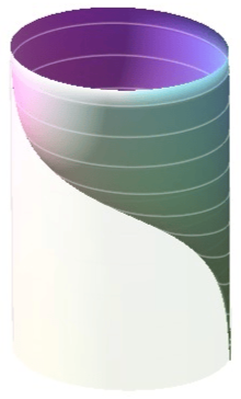
Figure 1. The depicted hypersurface, called a parabolic bowl, is a homogeneous entire vertical graph in $\mathbb{H}^{n}\times\mathbb{R}$ whose level hypersurfaces are parallel horospheres (we thank João P. dos Santos for this plot).

Inspired by Domínguez-Vázquez and Manzano’s work, we aim to establish here the following classification result for hypersurfaces of the products $\mathbb{Q}_{\epsilon}^{n}\times\mathbb{R}$, where $\mathbb{Q}_{\epsilon}^{n}$ stands for the $n(\geq 2)$-dimensional simply connected space form of constant sectional curvature $\epsilon=\pm 1$, that is, the hyperbolic space $\mathbb{H}^{n}$ for $\epsilon=-1$, and the sphere $\mathbb{S}^{n}$ for $\epsilon=1$:

Theorem 1.

Let $\varSigma$ be a connected hypersurface of  $\mathbb{Q}_{\epsilon}^{n}\times\mathbb{R}$. Then, the following assertions are equivalent:

1. $\varSigma$ is isoparametric.

2. $\varSigma$ has constant angle and constant principal curvatures.

3. $\varSigma$ is an open set of one of the following complete hypersurfaces:

   • a horizontal slice  $\mathbb{Q}_{\epsilon}^{n}\times\{t_{0}\}$,

   • a vertical cylinder over a complete isoparametric hypersurface of  $\mathbb{Q}_{\epsilon}^{n}$,

   • a parabolic bowl of $\mathbb{H}^{n}\times\mathbb{R}$ (see Fig. 1).

Moreover, the assertion

1. $\varSigma$ is an open set of a homogeneous hypersurface

is equivalent to the above assertions (i)–(iii) in the hyperbolic case $\epsilon=-1$. In the spherical case $\epsilon=1$, (iv) is equivalent to

1. $\varSigma$ is an open set of either a horizontal slice or a vertical cylinder over a complete homogeneous hypersurface of  $\mathbb{S}^{n}$.

The first part of Theorem 1 follows directly from Propositions 5–8 in Sections 3 and 4. For the second part, we have that (iv) implies (i) in any Riemannian manifold, as we mentioned before, and that horizontal slices are clearly homogeneous in $\mathbb{Q}_{\epsilon}^{n}\times\mathbb{R}$. For $\epsilon=-1$, we also have that parabolic bowls and vertical cylinders over isoparametric hypersurfaces are all homogeneous (see Proposition 5), so that (iii) implies (iv) for $\epsilon=-1$. For $\epsilon=1$, the equivalence between (iv) and (v) follows from the equivalence between (i) and (iii), and the fact that a vertical cylinder over a hypersurface $\varSigma_{0}$ of  $\mathbb{S}^{n}$ is homogeneous in the product $\mathbb{S}^{n}\times\mathbb{R}$ if and only if $\varSigma_{0}$ is homogeneous in the sphere $\mathbb{S}^{n}$.

The most delicate part of the proof of Theorem 1, which we do in Proposition 8, is showing that the connected isoparametric hypersurfaces of $\mathbb{Q}_{\epsilon}^{n}\times\mathbb{R}$ have constant angle function. To accomplish that, we proceed as Domínguez-Vázquez and Manzano in [17]. More precisely, we apply Jacobi field theory for reducing the proof to the resolution of an algebraic problem. In the $n$-dimensional setting, such problem is considerably more involved than its $2$-dimensional analogue, which compelled us to approach it differently. Our trick then was to consider an alternate problem on which the corresponding algebraic equations are all linear. In this way, the solution became attainable, although this new linear problem were still arduous (see Section 5).

For the remaining of the proof of Theorem 1, we apply some results obtained in [12, 32], including the one that characterizes constant angle hypersurfaces of the products $\mathbb{Q}_{\epsilon}^{n}\times\mathbb{R}$ as horizontal slices, vertical cylinders or vertical graphs built on parallel hypersurfaces of $\mathbb{Q}_{\epsilon}^{n}$ (cf. Sec. 2.2).

Theorem 1 provides an explicit classification of the isoparametric hypersurfaces and of the homogeneous hypersurfaces of $\mathbb{Q}_{\epsilon}^{n}\times\mathbb{R}$, since such classes of hypersurfaces are completely classified in $\mathbb{Q}_{\epsilon}^{n}$. The case $n=2$, of course, is contained in the main result by Domínguez-Vázquez and Manzano [17]. We included it here due to the fact that our proof differs from theirs in some substantial parts. For $n=3$, it was proved in [25] that hypersurfaces with constant principal curvatures have constant angle. Considering this result, we can drop the assumption on the constancy of the angle in Theorem 1 when $n=3$. Finally, we remark that Theorem 1 also gives that all isoparametric hypersurfaces of $\mathbb{Q}_{\epsilon}^{n}\times\mathbb{R}$ have constant scalar curvature, since the scalar curvature of a hypersurface of $\mathbb{Q}_{\epsilon}^{n}\times\mathbb{R}$ satisfies a relation (see, e.g., equality (6.2) in [10]) which implies that any such hypersurface having constant angle and constant principal curvatures is necessarily of constant scalar curvature.

2. Preliminaries

2.1. Hypersurfaces of $\mathbb{Q}_{\epsilon}^{n}\times\mathbb{R}$

Given an oriented hypersurface $\varSigma$ of $\mathbb{Q}_{\epsilon}^{n}\times\mathbb{R}$ (endowed with the standard product metric), set $N$ for its unit normal field and $A$ for its shape operator with respect to $N,$ that is

$$AX=-\mkern 1.5mu\overline{\mkern-1.5mu\nabla\mkern-1.5mu}\mkern 1.5mu_{X}N,\,\,\,X\in\mathfrak{X}(\varSigma),$$

where $\mkern 1.5mu\overline{\mkern-1.5mu\nabla\mkern-1.5mu}\mkern 1.5mu$ is the Levi-Civita connection of $\mathbb{Q}_{\epsilon}^{n}\times\mathbb{R},$ and $\mathfrak{X}(\varSigma)$ is the tangent bundle of $\varSigma$. The principal curvatures of $\varSigma,$ i.e., the eigenvalues of the shape operator $A,$ will be denoted by $k_{1}\,,\dots,k_{n}$. In this setting, the non-normalized mean curvature $H$ of $\varSigma$ is defined as the sum of its principal curvatures, that is,

$$H:=k_{1}+\cdots+k_{n}.$$

We define the height function $\phi$ and the angle function $\varTheta$ of $\varSigma$ as:

$$\phi:=\pi_{\scriptscriptstyle\mathbb{R}}|_{\varSigma}\quad\text{and}\quad\varTheta:=\langle N,\partial_{t}\rangle,$$

where $\partial_{t}$ denotes the gradient of the projection $\pi_{\scriptscriptstyle\mathbb{R}}$ of $\mathbb{Q}_{\epsilon}^{n}\times\mathbb{R}$ on its second factor $\mathbb{R}.$ Notice that $\partial_{t}$ is a unit parallel field on $\mathbb{Q}_{\epsilon}^{n}\times\mathbb{R}.$ Denoting by $\nabla$ the gradient on $C^{\infty}(\varSigma)$ and writing $T:=\nabla\phi,$ we have that the identity

$$T=\partial_{t}-\varTheta N$$

holds everywhere on $\varSigma.$ In particular, one has $\|T\|^{2}=1-\varTheta^{2}.$

2.2. Graphs on parallel hypersurfaces

Let $\mathscr{F}:=\{M_{s}\subset\mathbb{Q}_{\epsilon}^{n}\,;\,s\in I\}$ be a family of parallel hypersurfaces of $\mathbb{Q}_{\epsilon}^{n},$ where $I\subset\mathbb{R}$ is an open interval. Given a smooth function $\phi$ on $I,$ let

$$f\colon M_{s_{0}}\times I\rightarrow\mathbb{Q}_{\epsilon}^{n}\times\mathbb{R},\,\,\,s_{0}\in I,$$

be the immersion given by

$$f(p,s):=(\exp_{p}(s\eta_{s_{0}}(p)),\phi(s)),\,\,\,(p,s)\in M_{s_{0}}\times I,$$

where $\exp$ denotes the exponential map of $\mathbb{Q}_{\epsilon}^{n},$ and $\eta_{s_{0}}$ is the unit normal of $M_{s_{0}}.$ The hypersurface $\varSigma=f(M_{s_{0}}\times I)$ is a vertical graph over an open set of $\mathbb{Q}_{\epsilon}^{n}$ whose level hypersurfaces are the parallels $M_{s}$ to $M_{s_{0}}.$

Definition 2.

With the above notation, we call $\varSigma$ an $(M_{s},\phi)$-graph and say that

(1) $$\varrho(s):=\frac{\phi^{\prime}(s)}{\sqrt{1+(\phi^{\prime})^{2}(s)}},\,\,\,s\in I,$$

is the $\varrho$-function of $\varSigma$.

Given an $(M_{s},\phi)$-graph $\varSigma$ in $\mathbb{Q}_{\epsilon}^{n}\times\mathbb{R}$, it is easily seen that $N=-\varrho(s)\eta_{s}(p)+\varTheta\partial_{t}$ is a unit normal to it. In particular, one has that the equality

(2) $$\varrho^{2}+\varTheta^{2}=1$$

holds everywhere on $\varSigma$.

It was proved in [9] that, with this orientation, the principal curvature functions $k_{i}=k_{i}(p,s)$ of $\varSigma$ at a point $(p,s)\in M_{s_{0}}\times I$ are:

$$k_{i}=-\varrho(s)k_{i}^{s}(p),\,\,\,i\in\{1,\dots,n-1\},\quad\text{and}\quad k_{n}=\varrho^{\prime}(s),$$

where $k_{i}^{s}(p)$ is the $i$-th principal curvature of the parallel $M_{s}$ at $\exp_{p}(s\eta_{s_{0}}(p)).$

We point out that, from (1), one has

$$\phi(s)=\int_{s_{0}}^{s}\frac{\varrho(u)}{\sqrt{1-\varrho^{2}(u)}}du+\phi(s_{0}),\,\,\,s_{0},s\in I.$$

Hence, an $(M_{s},\phi)$ graph is determined by its $\varrho$-function.

3. Isoparametric hypersurfaces of constant angle

In this section, we prove Propositions 5 and 6, which establish the existence of the parabolic bowl as described in Figure 1, and its uniqueness (together with horizontal slices and vertical cylinders over isoparametric hypersurfaces of $\mathbb{Q}_{\epsilon}^{n}$) as a hypersurface of constant angle and constant principal curvatures in $\mathbb{Q}_{\epsilon}^{n}\times\mathbb{R}$. In the proofs, the following two lemmas will play a crucial role. They first appeared in [32], and later in [12] in a more general form. For notational purposes, we refer to the corresponding results of [12].

Lemma 3 (Theorem 7 of [12]).

Let $\{M_{s}\,;\,s\in I\}$ be a family of isoparametric hypersurfaces of  $\mathbb{Q}_{\epsilon}^{n}$. Consider the first order differential equation

(3) $$y^{\prime}=H^{s}y+H,\,\,\,s\in I,$$

where $H^{s}$ denotes the mean curvature of $M_{s}$ and $H$ is a constant. In this setting, if $\varrho\colon I\to(0,1)\subset\mathbb{R}$ is a solution to (3), then the $(M_{s},\phi)$-graph determined by $\varrho$ has constant mean curvature $H$. Conversely, if an $(M_{s},\phi)$-graph $\varSigma$ has constant mean curvature $H$, then $\{M_{s}\,;\,s\in I\}$ is isoparametric and the $\varrho$-function of $\varSigma$ is a solution to (3).

Lemma 4 (Corollary 4 of [12]).

Let $\varSigma$ be a connected hypersurface of  $\mathbb{Q}_{\epsilon}^{n}\times\mathbb{R}$ whose angle function is constant. Then, one of the following occurs:

• $\varSigma$ is an open set of a horizontal slice $\mathbb{Q}_{\epsilon}^{n}\times\{t_{0}\}$;

• $\varSigma$ is a vertical cylinder over a hypersurface of  $\mathbb{Q}_{\epsilon}^{n}$;

• $\varSigma$ is locally an $(M_{s},\phi)$-graph with $\phi^{\prime}$ a nonzero constant.

Now, we are in position to state and prove the announced Propositions 5 and 6.

Proposition 5.

Given $H\in(0,n-1)$, there exists an entire $(M_{s},\phi)$-graph $\varSigma_{H}$ in $\mathbb{H}^{n}\times\mathbb{R}$ (to be called a parabolic bowl) of constant mean curvature $H,$ which is homogeneous and has constant angle. In particular, $\varSigma_{H}$ is isoparametric and has constant principal curvatures.

Proof.

Let $\mathscr{F}:=\{M_{s}\,;\,s\in\mathbb{R}\}$ be a family of parallel horospheres of $\mathbb{H}^{n}$. Then, considering the “outward orientation” in each $M_{s}$, for all $s\in\mathbb{R}$ and all $p\in M_{s}$, we have that $k_{i}^{s}(p)=-1$ for all $i\in{1,\dots,n-1}$. Therefore, given $H\in(0,n-1)$, the ODE (3) associated to $\mathscr{F}$ and $H$ is

(4) $$y^{\prime}=-(n-1)y+H.$$

Clearly, the constant function $\varrho=H/(n-1)<1$ is a solution to (4). Hence, by Lemma 3, the entire $(M_{s},\phi)$-graph $\varSigma_{H}$ of $\mathbb{H}^{n}\times\mathbb{R}$ which is determined by $\varrho$ has constant mean curvature $H$. Moreover, by (2), $\varSigma_{H}$ has constant angle function.

Finally, the homogeneity of $\varSigma_{H}$ follows from its invariance by the one parameter group of parabolic translations of $\mathbb{H}^{n}$ which fix each horosphere $M_{s}$ (extended slicewise to $\mathbb{H}^{n}\times\mathbb{R}$), as well as by the isometries $\Psi_{u}\times\uptau_{u}$, $u\in\mathbb{R},$ where

$$\{\Psi_{u}\,;\,u\in\mathbb{R}\}\subset{\rm Iso}(\mathbb{H}^{n})$$

is the flow defined by the unit normals of the horospheres $M_{s}$, and $\uptau_{u}$ is the vertical translation $(p,t)\mapsto(p,t+\varrho u)$ of $\mathbb{H}^{n}\times\mathbb{R}.$ ∎

When $n=2$, our parabolic bowl $\varSigma_{H}$ corresponds to the surface $P_{H,-1,0}$ of [17], and to the surface $P_{H}$ of [24]. They also appear in [25], for $n=3$, and in [7], for $n\geq 2$. In all of these occurrences, the hypersurface is under no specific designation, except in [17], where they are called parabolic helicoids. Our chosen nomenclature comes from the extrinsic geometric flows theory, for it was shown in [11] that, for each $r\in\{1,\dots,n-1\}$, there exists a parabolic bowl $\varSigma_{H_{r}}$ of constant $r$-th mean curvature $H_{r}$ such that $H_{r}=\varTheta$ on $\varSigma_{H_{r}}$. As a consequence, $\varSigma_{H_{r}}$ is a translating soliton to mean curvature flow of $r$-th order. In this context, entire graphs with this property are called bowl solitons. We should also mention that any parallel to a given parabolic bowl is nothing but a vertical translation of it. Therefore, analogously to the slices $\mathbb{H}^{n}\times\{t\}$, $t\in\mathbb{R}$, the family of all parallels to a parabolic bowl defines a nonsingular isoparametric foliation of $\mathbb{H}^{n}\times\mathbb{R}$.

Proposition 6.

Let $\varSigma$ be a connected hypersurface of  $\mathbb{Q}_{\epsilon}^{n}\times\mathbb{R}$ with constant angle function. Then, $\varSigma$ is isoparametric if and only if it has constant principal curvatures. If so, $\varSigma$ is an open set of one of the following hypersurfaces:

• a horizontal slice  $\mathbb{Q}_{\epsilon}^{n}\times\{t_{0}\}$,

• a vertical cylinder over a complete isoparametric hypersurface of  $\mathbb{Q}_{\epsilon}^{n}$,

• a parabolic bowl if $\epsilon=-1$.

Proof.

By Lemma 4, $\varSigma$ is an open set of a horizontal slice, a vertical cylinder over a hypersurface of $\mathbb{Q}_{\epsilon}^{n}$, or is locally an $(M_{s},\phi)$-graph such that $\phi^{\prime}$ is constant. If the first occurs, we are done. Assume then that $\varSigma$ is a cylinder $\varSigma_{0}\times\mathbb{R}$, where $\varSigma_{0}$ is a hypersurface of $\mathbb{Q}_{\epsilon}^{n}$. It is easily seen that $\varSigma$ is isoparametric (resp. has constant principal curvatures) if and only if $\varSigma_{0}$ is isoparametric (resp. has constant principal curvatures). However, in $\mathbb{Q}_{\epsilon}^{n},$ to be isoparametric and to have constant principal curvatures are equivalent conditions. Besides, we have from the classification of isoparametric hypersurfaces of space forms that any isoparametric hypersurface of $\mathbb{Q}_{\epsilon}^{n}$ is necessarily an open set of a complete isoparametric hypersurface.

Let us suppose now that $\varSigma$ is locally an $(M_{s},\phi)$-graph of $\mathbb{Q}_{\epsilon}^{n}\times\mathbb{R}$, $s\in I$, such that $\phi^{\prime}$ is a nonzero constant. Then, from (1), the $\varrho$-function of $\varSigma$ is a nonzero constant as well. If either $\varSigma$ is isoparametric or has constant principal curvatures, then its mean curvature $H$ is constant. In this case, it follows from Lemma 3 that the hypersurfaces $M_{s}$ are isoparametric and that $\varrho$ satisfies $0=\varrho^{\prime}=\varrho H^{s}+H,$ which implies that the mean curvature $H^{s}$ of $M_{s}$ is a constant independent of $s$. Again, by considering the classification of isoparametric hypersurfaces of $\mathbb{Q}_{\epsilon}^{n}$, one concludes that $\{M_{s}\,;\,s\in I\}$ is necessarily a family of parallel horospheres of $\mathbb{H}^{n}$, so that $\varSigma$ is an open set of a parabolic fun of $\mathbb{H}^{n}\times\mathbb{R}$. ∎

Remark 7.

The first part of Proposition 6 is essentially the content of Corollary 5.2 of [7]. Nonetheless, the proof which is given there is rather distinct from ours.

4. The constancy of the angle function

This section will be entirely dedicated to the proof of the following proposition, which constitutes our main result for establishing Theorem 1.

Proposition 8.

The angle function of any connected isoparametric hypersurface of  $\mathbb{Q}_{\epsilon}^{n}\times\mathbb{R}$ is constant.

Given a field $X\in\mathfrak{X}(\mathbb{Q}_{\epsilon}^{n}\times\mathbb{R})$, we shall denote by $X^{h}$ its component which is tangent to $\mathbb{Q}_{\epsilon}^{n}$ (called horizontal), that is,

$$X^{h}:=X-\langle X,\partial_{t}\rangle\partial_{t}.$$

When $X=X^{h}$, we say that the field $X$ is horizontal.

Since the first factor of $\mathbb{Q}_{\epsilon}^{n}\times\mathbb{R}$ has constant sectional curvature $\epsilon$ and its second factor is one-dimensional, the Riemannian curvature tensor $R_{\epsilon}$ of $\mathbb{Q}_{\epsilon}^{n}\times\mathbb{R}$ is

$$R_{\epsilon}(X,Y)Z=\epsilon(\langle X^{h},Z^{h}\rangle Y^{h}-\langle Y^{h},Z^{h}\rangle X^{h})\,\,\,\,\,\forall X,Y,Z\in\mathfrak{X}(\mathbb{Q}_{\epsilon}^{n}\times\mathbb{R}).$$

Proof of Proposition 8.

Let $\varSigma$ be a connected oriented isoparametric hypersurface of $\mathbb{Q}_{\epsilon}^{n}\times\mathbb{R}$. Since its angle function $\varTheta$ is continuous, it suffices to prove that $\varTheta$ is locally constant on $\varSigma$. We can assume that $\varTheta^{2}\neq 1$, so that the gradient $T$ of the height function of $\varSigma$ never vanishes. In this setting, define $\Phi^{r}\colon\varSigma\to\mathbb{Q}_{\epsilon}^{n}\times\mathbb{R}$ by

$$\Phi^{r}(p)=\exp_{p}(rN_{p}),$$

where $N_{p}$ is the unit normal field of $\varSigma$ at $p\in\varSigma$ and $\exp$ stands for the exponential map of $\mathbb{Q}_{\epsilon}^{n}\times\mathbb{R}$. Passing to an open subset of $\varSigma$, we can assume that, for a small $\delta>0,$ and for all $r\in(-\delta,\delta),$ the map $\Phi^{r}$ is well defined and $\varSigma_{r}:=\Phi^{r}(\varSigma)$ is an embedded hypersurface of $\mathbb{Q}_{\epsilon}^{n}\times\mathbb{R}$ which lies at distance $|r|$ from $\varSigma$.

Given $p\in\varSigma$, let $\gamma_{p}(r)$ be the geodesic of $\mathbb{Q}_{\epsilon}^{n}\times\mathbb{R}$ such that $\gamma_{p}(0)=p$ and $\gamma_{p}^{\prime}(0)=N_{p}$, that is, $\gamma_{p}(r)=\Phi^{r}(p)$. It is easily seen that the unit normal to $\varSigma^{r}$ at $\gamma_{p}(r)$ is $N(r):=\gamma_{p}^{\prime}(r)$. In particular, $N(r)$ is parallel along $\gamma_{p}$. Since $\partial_{t}$ is parallel on $\mathbb{Q}_{\epsilon}^{n}\times\mathbb{R}$, this gives that the angle function of $\varSigma_{r}$ is constant along $\gamma_{p}$. Consequently, the gradient of the height function of $\varSigma_{r}$ at $\gamma_{p}(r)$ is the parallel transport $T(r)$ of $T$ along $\gamma_{p}$.

Set $U_{1}(r)=T(r)/|T(r)|$ and let $N(r),U_{1}(r),U_{2}(r),\dots,U_{n}(r)$ be an orthonormal parallel frame along $\gamma_{p}$. Notice that, for all $i\in\{2,\dots,n\}$, $U_{i}(r)$ is horizontal. Indeed, for such an $i$, $0=\langle U_{i}(r),T(r)\rangle=\langle U_{i},\partial_{t}\rangle.$

For any $j\in\{1,\dots,n\}$, let $\zeta_{j}=\zeta_{j}(r)$ be the Jacobi field along $\gamma_{p}$ such that

(5) $$\zeta_{j}(0)=U_{j}(0)\quad\text{and}\quad\zeta^{\prime}_{j}(0)=-AU_{j}(0),$$

where $A$ is the shape operator of $\varSigma$. Then, for any such $j$, $\zeta_{j}$ satisfies

(6) $$\zeta_{j}^{\prime\prime}+R_{\epsilon}(\zeta_{j},\gamma_{p}^{\prime})\gamma_{p}^{\prime}=0.$$

In addition, for all $r\in(-\delta,\delta),$ one has $\langle\zeta_{j}(r),N(r)\rangle=0$. Therefore, there exist smooth functions $b_{ij}=b_{ij}(r)$ such that

(7) $$\zeta_{j}=\sum_{i=1}^{n}b_{ij}U_{i},\,\,\,j\in\{1,\dots,n\}.$$

Furthermore, since all $U_{i}$ are parallel along $\gamma_{p}$, we have

(8) $$\zeta^{\prime\prime}_{j}=\sum_{i=1}^{n}b_{ij}^{\prime\prime}U_{i},\,\,\,j\in\{1,\dots,n\}.$$

Now, aiming the Jacobi equation (6), we compute

(9) $$R_{\epsilon}(\zeta_{j},\gamma_{p}^{\prime})\gamma_{p}^{\prime}=R_{\epsilon}(\zeta_{j},N)N=\epsilon(\langle\zeta_{j}^{h},N^{h}\rangle N-\langle N^{h},N^{h}\rangle\zeta_{j}^{h}).$$

However, $N^{h}=N-\varTheta\partial_{t},$ so that $\langle N^{h},N^{h}\rangle=1-\varTheta^{2}$. Besides, considering (7) and the fact that $U_{i}$ is horizontal for all $i\geq 2$, we have:

$$\zeta_{j}^{h}=\zeta_{j}-\langle\zeta_{j},\partial_{t}\rangle\partial_{t}=\zeta_{j}-b_{1j}\langle U_{1},\partial_{t}\rangle=\zeta-b_{1j}\|T\|\partial_{t}.$$

In particular,

$$\langle\zeta_{j}^{h},N^{h}\rangle=\langle\zeta_{j}-b_{1j}\|T\|\partial_{t},N-\varTheta\partial_{t}\rangle=-\varTheta\langle\zeta_{j},\partial_{t}\rangle=-\varTheta\|T\|b_{1j}.$$

It follows from (9) and the above equalities that,

$$\epsilon R_{\epsilon}(\zeta_{j},\gamma_{p}^{\prime})\gamma_{p}^{\prime} = -\varTheta b_{1j}\|T\|N-(1-\varTheta^{2})\zeta_{j}+b_{ij}\|T\|\partial_{t}=b_{1j}\|T\|T-(1-\varTheta^{2})\zeta_{j}$$

$$= \sum_{i=2}^{n}-(1-\varTheta^{2})b_{ij}U_{i}.$$

This last equality and (6) then give

(10) $$\zeta_{j}^{\prime\prime}=\sum_{i=2}^{n}\epsilon(1-\varTheta^{2})b_{ij}U_{i}.$$

Now, set $(a_{ij})$ for the (symmetric) matrix of $A$ with respect to the orthonormal basis $\{U_{1}(0),\dots,U_{n}(0)\}$, that is,

$$AU_{j}(0)=\sum_{i=1}^{n}a_{ij}U_{i}(0).$$

Considering this last equality and comparing (8) with (10), we conclude that $\zeta_{j}$ is a Jacobi field satisfying the initial conditions (5) if and only if the coefficients $b_{ij}$ are solutions of a initial value problem. Namely,

(11) $$\left\{\begin{array}[]{rcll}b_{1j}^{\prime\prime}(r)&=&0;\\[4.30554pt] b_{ij}^{\prime\prime}(r)&=&\epsilon(1-\varTheta^{2})b_{ij}(r),&\text{if}\ i\geq 2;\\[4.30554pt] b_{ij}(0)&=&\delta_{ij};\\[4.30554pt] b_{ij}^{\prime}(0)&=&-a_{ij}.\end{array}\right.$$

Defining

$$\uptau:=\epsilon(1-\varTheta^{2})\neq 0,$$

the solutions of (11) are

(12) $$\left\{\begin{array}[]{rcll}b_{1j}(r)&=&\delta_{1j}-a_{1j}r;\\[4.30554pt] b_{ij}(r)&=&\delta_{ij}c_{\uptau}(r)-a_{ij}s_{\uptau}(r)&\text{if}\ i\geq 2;\end{array}\right.$$

where $s_{\uptau}$ and $c_{\uptau}$ are the functions:

(13) $$s_{\uptau}(r):=\left\{\begin{array}[]{lcc}\frac{1}{\sqrt{\uptau}}\sinh(\sqrt{\uptau}\,r)&\text{if}&\uptau>0,\\[4.30554pt] \frac{1}{\sqrt{-\uptau}}\sin(\sqrt{-\uptau}\,r)&\text{if}&\uptau<0,\end{array}\right.\quad c_{\uptau}(r):=\left\{\begin{array}[]{lcc}\cosh(\sqrt{\uptau}\,r)&\text{if}&\uptau>0,\\[4.30554pt] \cos(\sqrt{-\uptau}\,r)&\text{if}&\uptau<0.\end{array}\right.$$

Notice that the derivatives of $s_{\uptau}$ and $c_{\uptau}$ satisfy:

(14) $$s_{\uptau}^{\prime}(r)=c_{\uptau}(r)\quad\text{and}\quad c_{\uptau}^{\prime}(r)=\uptau s_{\uptau}(r)\,\,\,\forall r\in\mathbb{R}.$$

Given $r\in(-\delta,\delta),$ let $B(r)$ and $C(r)$ be the linear operators of $T_{\gamma_{p}(r)}\varSigma_{r}$ which take the basis $\{U_{1}(r),\dots,U_{n}(r)\}$ to $\{\zeta_{1}(r),\dots,\zeta_{n}(r)\}$ and $\{\zeta_{1}^{\prime}(r),\dots,\zeta_{n}^{\prime}(r)\},$ respectively. Considering (7) and the fact that each $U_{i}$ is parallel along $\gamma_{p}$, we conclude that their matrices with respect to this basis are

$$B(r)=(b_{ij}(r))\quad\text{and}\quad C(r)=(b_{ij}^{\prime}(r)),\,\,\,i,j\in\{1,\dots,n\},$$

where $b_{ij}$ are the functions defined in (12).

In the above setting, Jacobi field theory applies, giving that $B(r)$ is nonsingular for each $r\in(-\delta,\delta)$, and that the shape operator of $\varSigma^{r}$ is $A^{r}=-C(r)B(r)^{-1}$ (see [1, Theorem 10.2.1]). In particular,

$$H(r)={\rm trace}\,A^{r}=-{\rm trace}\,(C(r)B(r)^{-1})=-\frac{\frac{d}{dr}(\det B(r))}{\det B(r)},$$

where, in the last equality, we used the fact that $\nabla\det(B)=(\det B){\rm adj}(B^{-1}).$

Defining $D(r)=\det B(r)$, it follows from the above that the function

$$f(r)=D^{\prime}(r)+H(r)D(r)$$

vanishes identically. Since $D^{\prime}=f-HD=-HD$, one has

$$f^{\prime}=D^{\prime\prime}+H^{\prime}D+HD^{\prime}=D^{\prime\prime}+(H^{\prime}-H^{2})D.$$

Therefore, for all $k\in\mathbb{N}$,

(15) $$0=f^{(k)}=D^{(k+1)}+\phi_{k}D,\quad\phi_{k}=\phi_{k}(H,H^{\prime},\dots,H^{(k)}),$$

where $f^{(k)}$ denotes the $k$-th derivative of $f$.

Now, considering that the functions $b_{ij}(r)$ are as in (12), we decompose the matrix $B(r)=(b_{ij}(r))$ in blocks as

(16) $$B(r)=\left[\begin{array}[]{c|c}1-a_{11}r&\begin{array}[]{ccc}-a_{12}r&\dots&-a_{1n}r\end{array}\\ \hline\cr\begin{array}[]{c}-a_{12}s_{\uptau}(r)\\ \vdots\\ -a_{1n}s_{\uptau}(r)\end{array}&\delta_{ij}c_{\uptau}(r)-a_{ij}s_{\uptau}(r)\end{array}\right].$$

Expanding $D(r)=\det B(r)$ with respect to the first row of $B(r)$ and considering the equalities (14), one can easily prove by induction that, for any integers $n\geq 2$ and $k\geq 1$, and for any $\ell\in\{0,\dots,n-1\}$, there are coefficients $\alpha_{\ell,k},\beta_{\ell,k}$, which do not depend on $r$, such that

(17) $$D^{(k)}(r)=\sum_{\ell=0}^{n-1}(\alpha_{\ell,k}+\beta_{\ell,k}r)s_{\uptau}^{\ell}(r)c_{\uptau}^{n-1-\ell}(r).$$

Taking the first $2n-1$ derivatives of the (constant) function $f$ at $r=0$ and using (15) and (17), we conclude that

(18) $$0=f^{(k)}(0)=\alpha_{0,k+1}(0)+d_{k}\,\,\,\text{for any}\ k\in\{1,\dots,2n-1\},$$

where $d_{k}=\phi_{k}(H(0),H^{\prime}(0),\dots,H^{(k)}(0)).$ In addition, as shown in Lemma 10 of the appendix, the coefficients $\alpha_{\ell,k}$ and $\beta_{\ell,k}$ satisfy recursive equations which allow us to express each of them in terms of $\alpha_{\ell,0}$ and $\beta_{\ell,0}.$ In this way, for any $k\in\mathbb{N}$, after $k+1$ steps, we can write $\alpha_{0,k+1}$ as the linear combination

(19) $$\alpha_{0,k+1}=\sum_{\ell=0}^{n-1}(p_{k+1,\ell}\alpha_{\ell,0}+q_{k+1,\ell}\beta_{\ell,0}),$$

where the coefficients $p_{k+1,\ell}$ and $q_{k+1,\ell}$ depend only on $k$, $n$, $\ell$, and $\uptau$. Moreover, we have that $\alpha_{0,0}=D(0)=1$ and, by (18), that $\alpha_{0,k+1}$ coincides with the constant $d_{k}$. Therefore, the vector

$$x_{0}=(\alpha_{1,0},\dots,\alpha_{n-1,0},\beta_{0,0},\dots,\beta_{n-1,0})$$

is a solution to the linear system

(20) $$Mx=P,\quad x\in\mathbb{R}^{2n-1},$$

whose augmented matrix $[M|P]$ has vector rows $L_{1},\dots,L_{2n-1}\in\mathbb{R}^{2n}$, where

$$L_{k}:=(p_{k+1,1},p_{k+1,2},\dots,p_{k+1,n-1},q_{k+1,0},q_{k+1,1},\dots,q_{k+1,n-1},d_{k}-p_{k+1,0}).$$

In what follows, by means of a thorough analysis of the system (20), we shall show that $\uptau=\uptau(p)$ is necessarily a root of a polynomial equation, and so $\uptau$ must be constant on $\varSigma$. To that end, it will be convenient to consider first the cases $n=2$ and $n=3$.

Case 1: $n=2$.

As we mentioned before, this case was considered in [17]. We include it here to better illustrate our strategy, which is distinct from the one employed there.

For $n=2$, the equalities of Lemma 10 in the appendix yield

• $\alpha_{0,2}=2\beta_{1,0}+\uptau\alpha_{0,0}$;

• $\alpha_{0,3}=\uptau\alpha_{1,0}+3\uptau\beta_{0,0}$;

• $\alpha_{0,4}=4\uptau\beta_{1,0}+\uptau^{2}\alpha_{0,0}$.

These equalities imply that the augmented matrix $[M|P]$ of the system (20) is

$$[M|P]=\left[\begin{array}[]{ccc|c}0&0&2&d_{1}-\uptau\\ \uptau&3\uptau&0&d_{2}\\ 0&0&4\uptau&d_{3}-\uptau^{2}\end{array}\right],$$

where $d_{i}=-\phi_{i}(0)$, $i\in\{1,2,3\}.$ However, it is easily seen that $\det M=0$. Hence, denoting by $M_{j}$ the matrix obtained from $M$ by replacing its $j$-th column by $P$, we have that $\det M_{j}=0$ for all $j\in\{1,2,3\}$. Otherwise, by Crammer’s rule, the system $Mx=P$ would have no solution, thereby contradicting the existence of the solution $x_{0}=(\alpha_{1,0},\beta_{0,0},\beta_{1,0}).$ In particular, we have

(21) $$0=\det M_{2}=2\uptau^{3}-4d_{1}\uptau^{2}+2d_{3}\uptau,$$

so that $\uptau$ is a root of a polynomial equation. This proves Proposition 8 for $n=2$.

Case 2: $n=3$.

Firstly, we point out that, as shown in Proposition 11 in the appendix, the following equalities hold:

• $L_{2s-1}=(0,2^{2s-1}\uptau^{s-1},0,s2^{2s-1}\uptau^{s-1},0,d_{2s-1}-2^{2s-1}\uptau^{s})$;

• $L_{2s}=(2^{2s}\uptau^{s},0,(2s+1)2^{2s-1}\uptau^{s},0,(2s+1)2^{2s-1}\uptau^{s-1},d_{2s})$.

Proceeding as in the previous case, we conclude that, for $n=3$, the augmented matrix $[M|P]$ is

$${\small[M|P]=\left[\begin{array}[]{ccccc|c}0&2&0&2&0&d_{1}-2\uptau\\ 4\uptau&0&6\uptau&0&6&d_{2}\\ 0&8\uptau&0&16\uptau&0&d_{3}-8\uptau^{2}\\ 16\uptau^{2}&0&40\uptau^{2}&0&40\uptau&d_{4}\\ 0&32\uptau^{2}&0&96\uptau^{2}&0&d_{5}-32\uptau^{3}\\ \end{array}\right]}.$$

Again, we have $\det M=0,$ so that $\det M_{j}=0$ for any $j\in\{1,\dots,5\}$, for

$$x_{0}=(\alpha_{1,0},\alpha_{2,0},\beta_{0,0},\beta_{1,0},\beta_{2,0})$$

is a solution to (20). Since the 3-th and 5-th column vectors of $M$ are linearly dependent, for $j\notin\{3,5\},$ the equality $\det M_{j}=0$ holds for any $\uptau$. On the other hand, a direct computation gives

(22) $$\det M_{5}=-\det M_{3}=d_{1}2^{14}\uptau^{6}-d_{3}2^{13}\uptau^{5}+d_{5}2^{10}\uptau^{4}.$$

Thus, if $d_{1},d_{3}$ and $d_{5}$ are not all zero, any of the equalities $\det M_{j}=0$, $j\in\{3,5\}$, gives that $\uptau$ is a nonzero root of a polynomial equation. However, if $d_{1}=d_{3}=d_{5}=0$, the determinants of all $M_{j}$ will vanish identically. To overcome this problem, we replace the system $Mx=P$ by a suitable system $\mkern 1.5mu\overline{\mkern-1.5muM\mkern-1.5mu}\mkern 1.5mux=\mkern 1.5mu\overline{\mkern-1.5muP\mkern-1.5mu}\mkern 1.5mu$ as follows.

Given $s>3,$ consider the system $\mkern 1.5mu\overline{\mkern-1.5muM\mkern-1.5mu}\mkern 1.5mux=\mkern 1.5mu\overline{\mkern-1.5muP\mkern-1.5mu}\mkern 1.5mu$, where $[\mkern 1.5mu\overline{\mkern-1.5muM\mkern-1.5mu}\mkern 1.5mu|\mkern 1.5mu\overline{\mkern-1.5muP\mkern-1.5mu}\mkern 1.5mu]$ is obtained from $[M|P]$ by replacing its fifth row vector $L_{5}$ by $L_{2s-1}$. The above reasoning applied to $\mkern 1.5mu\overline{\mkern-1.5muM\mkern-1.5mu}\mkern 1.5mux=\mkern 1.5mu\overline{\mkern-1.5muP\mkern-1.5mu}\mkern 1.5mu$ leads to the same conclusion: if $d_{1},d_{3}$ and $d_{2s-1}$ are not all zero, then $\uptau$ is a nonzero root of a polynomial equation. Therefore, we can assume that $d_{k}=0$ for all odd $k\geq 1.$

Now, given $s>2$, consider the system $\mkern 1.5mu\overline{\mkern-1.5muM\mkern-1.5mu}\mkern 1.5mux=\mkern 1.5mu\overline{\mkern-1.5muP\mkern-1.5mu}\mkern 1.5mu$, where $[\mkern 1.5mu\overline{\mkern-1.5muM\mkern-1.5mu}\mkern 1.5mu|\mkern 1.5mu\overline{\mkern-1.5muP\mkern-1.5mu}\mkern 1.5mu]$ is obtained from $[M|P]$ by replacing its fifth row vector $L_{5}$ by $L_{2s}.$ Setting

$$\lambda=2^{2s}\uptau^{s},\quad\mu=(2s+1)2^{2s-1}\uptau^{s}\quad\text{and}\quad\nu=(2s+1)2^{2s-1}\uptau^{s-1},$$

$[\mkern 1.5mu\overline{\mkern-1.5muM\mkern-1.5mu}\mkern 1.5mu|\mkern 1.5mu\overline{\mkern-1.5muP\mkern-1.5mu}\mkern 1.5mu]$ takes the form

$${\small[\mkern 1.5mu\overline{\mkern-1.5muM\mkern-1.5mu}\mkern 1.5mu|\mkern 1.5mu\overline{\mkern-1.5muP\mkern-1.5mu}\mkern 1.5mu]=\left[\begin{array}[]{ccccc|c}0&2&0&2&0&d_{1}-2\uptau\\ 4\uptau&0&6\uptau&0&6&d_{2}\\ 0&8\uptau&0&16\uptau&0&d_{3}-8\uptau^{2}\\ 16\uptau^{2}&0&40\uptau^{2}&0&40\uptau&d_{4}\\ \lambda&0&\mu&0&\nu&d_{2s}\\ \end{array}\right]}.$$

Noticing that $\nu\uptau=\mu$, one has $\det\mkern 1.5mu\overline{\mkern-1.5muM\mkern-1.5mu}\mkern 1.5mu=2^{14}\uptau^{3}(\nu\uptau-\mu)=0$. Hence, since $x_{0}$ is also a solution to $\mkern 1.5mu\overline{\mkern-1.5muM\mkern-1.5mu}\mkern 1.5mux=\mkern 1.5mu\overline{\mkern-1.5muP\mkern-1.5mu}\mkern 1.5mu$, we must have for any $s>2$ that

(23) $$0=\det\mkern 1.5mu\overline{\mkern-1.5muM\mkern-1.5mu}\mkern 1.5mu_{3}=d_{2}(2-s)2^{2s+8}\uptau^{s+2}+d_{4}(s-1)2^{2s+6}\uptau^{s+1}-d_{2s}2^{10}\uptau^{3}.$$

As before, it follows from the above that, if $d_{2},d_{4}$ and $d_{2s}$ are not all zero, then $\uptau$ is a nonzero root of a polynomial equation. So, we can assume that $d_{2s}=0$ for all $s\geq 1$.

To finish the proof in this present case, we show now that the assumption $d_{k}=0$ for all $k\geq 1$ leads to a contradiction. With this purpose, we first observe that, considering the expression of $B(r)$ in (16), a direct computation gives

$$D(r)=\mu_{1}(r)c_{\uptau}^{2}(r)+\mu_{2}(r)s_{\uptau}(r)c_{\uptau}(r)+\mu_{3}(r)s_{\uptau}^{2}(r),$$

where, for any $i\in\{1,2,3\}$, $\mu_{i}$ is an affine function of $r$.

On the other hand, under our assumption on the constants $d_{k}$, it follows from (15) that $D^{(k+1)}(0)=0$ for all $k\geq 1.$ Since $D(0)=1$ and $D$ is clearly a real analytic function of $r$, this implies that $D(r)-D(0)$ is a linear function of $r$ in a neighborhood of $r=0$, which is a contradiction. This proves Proposition 8 in the case $n=3$.

Next, we consider the general case $n>3$. Our task now is to show that the $(2n-1)\times 2n$ augmented matrix $[M|P]$ has the same fundamental properties as the ones for the cases $n=2$ and $n=3$ that implied the polynomial identities (21) (for $n=2$) and (22)-(23) (for $n=3$). As suggested by these particular cases, to get similar identities in the general case $n>3$, we have to consider just one linear system if $n$ is even, and infinitely many of them if $n$ is odd. This, of course, makes the former case much simpler.

In Proposition 9 below, we establish the aforementioned fundamental properties of $[M,P]$ for $n>3$. Its proof constitutes a challenging problem which we solve through a series of lemmas and propositions that are presented in the appendix.

We shall denote by $M(s)$ the $(2n-1)\times(2n-1)$ matrix obtained from $Z(s)$ (as defined in the statement of Proposition 18-(ii) in the appendix) by exclusion of its first column.

Proposition 9.

The matrices $M$ and $M(s)$ have the following properties:

• If $n$ is even, one has:

  • $M$ has rank $2n-2$;

  • there exists $j_{*}\in\{1,\dots,2n-1\}$ such that

    $$\det M_{j_{*}}=\mu_{0}\uptau^{\frac{\gamma_{0}}{2}}+\sum_{i=1}^{2n-1}\mu_{i}d_{i}\uptau^{\frac{\gamma_{i}}{2}},$$

    where $\mu_{0}\neq 0,\mu_{1},\dots,\mu_{2n-1}$ and $\gamma_{0}>\gamma_{1}>\dots>\gamma_{2n-1}>0$ are all integers.

• If $n$ is odd, for any $s\geq 2n$, one has:

  • $M(s)$ has rank $2n-2$;

  • the determinant of $M_{n}(s)$ is given by

    $$\det M_{n}(s)=\mu_{s}d_{s}\uptau^{\frac{\gamma_{s}}{2}}+\sum_{i=1}^{2n-2}\mu_{i}d_{i}\uptau^{\frac{\gamma_{i}}{2}},$$

    where $\mu_{1},\dots,\mu_{2n-2},\mu_{s}\neq 0$ and $\gamma_{1}>\dots>\gamma_{2n-2}>\gamma_{s}>0$ are all integers.

For a proper application of Proposition 9, we separate the proof of the general case $n>3$ into two parts.

Case 3: $n>3$, $n$ even.

It follows from Proposition 9-(i)-(a) that $\det M=0$. Since $x_{0}$ is a solution to $Mx=P$, we must have $\det M_{j}=0$ for all $j\in\{1,\dots,2n-1\}$. Now, let $j=j_{*}$ be the index as in Proposition 9-(i)-(b). Then $\det M_{j_{*}}=0$ is a non-trivial algebraic equation in the variable $\uptau$.

Case 4: $n>3$, $n$ odd.

Suppose that $d_{s}=0$ for any $s\geq 2n$. Then, as it was for $n=3$, we would have that $D$ is a polynomial function in a neighborhood of $r=0$, since $D$ is real analytic. However, it is clear from its expression in (16) that $D(r)$ coincides with no polynomial in such a neighborhood. Therefore, there exists $s_{*}\geq 2n$ such that $d_{s_{*}}\neq 0$. Proposition 9-(ii)-(a) then says that $\det M(s_{*})=0$. So, similarly to the previous case, $\det M_{j}(s_{*})=0$ for all $j\in\{1,\dots,2n-1\}$. Finally, item (b) of Proposition 9-(ii) gives that the equality $\det M_{n}(s_{*})=0$ is a non-trivial algebraic equation in $\uptau$.

This concludes the proof of Proposition 8. ∎

5. Appendix

In this appendix, we prove some results which we have used in the proof of Proposition 8. We keep the notation of the preceding section.

To start with, define the row vector

(24) $$\mathfrak{L}_{k-1}=(p_{k,0},\dots,p_{k,n-1},q_{k,0},\dots,q_{k,n-1}),\,\,\,k\geq 2,$$

and denote by $Z=[p_{k,\ell},q_{k,\ell}]$ the $(2n-1)\times 2n$ matrix with rows $\mathfrak{L}_{k-1}$, $2\leq k\leq 2n$:

(25) $$Z=[p_{k,\ell},q_{k,\ell}]=\begin{bmatrix}\mathfrak{L}_{1}\\ \vdots\\ \mathfrak{L}_{2n-1}\end{bmatrix}.$$

Our interest in the matrix $Z$ relies on the equality $Z=[-P_{\uptau},M],$ where

(26) $$P_{\uptau}:=P-P_{d},\quad P_{d}=\begin{bmatrix}d_{1}\\ d_{2}\\ \vdots\\ d_{2n-1}\end{bmatrix}.$$

In what follows, we establish a series of lemmas that will lead to a complete description of $Z$ (see Propositions 11 and 14).

Lemma 10.

Let $\alpha_{\ell,k}$ and $\beta_{\ell,k}$ be the coefficient functions defined in (17), that is,

(27) $$D^{(k)}(r)=\sum_{\ell=0}^{n-1}(\alpha_{\ell,k}+\beta_{\ell,k}r)s_{\uptau}^{\ell}(r)c_{\uptau}^{n-1-\ell}(r).$$

Then, for any $n,k\in\mathbb{N}$, the following equalities hold:

$$\left.\begin{array}[]{lcll}\alpha_{0,k+1}&=&\beta_{0,k}+\alpha_{1,k};\\[3.01385pt] \alpha_{\ell,k+1}&=&\beta_{\ell,k}+(\ell+1)\alpha_{\ell+1,k}+\uptau(n-\ell)\alpha_{\ell-1,k}&\text{if}\ \ell\in\{1,\dots,n-2\};\\[3.01385pt] \alpha_{n-1,k+1}&=&\beta_{n-1,k}+\uptau\alpha_{n-2,k};\\[3.01385pt] \\ \beta_{0,k+1}&=&\beta_{1,k};\\[3.01385pt] \beta_{\ell,k+1}&=&(\ell+1)\beta_{\ell+1,k}+\uptau(n-\ell)\beta_{\ell-1,k}&\text{if}\ \ell\in\{1,\dots,n-2\};\\[3.01385pt] \beta_{n-1,k+1}&=&\uptau\beta_{n-2,k}.\\[3.01385pt] \end{array}\right.$$

Proof.

Considering (27), we have that

$$D^{(k+1)}(r) = \sum_{\ell=0}^{n-1}\left[\beta_{\ell,k}s_{\uptau}^{\ell}(r)c_{\uptau}^{n-1-\ell}(r)+\ell(\alpha_{\ell,k}+\beta_{\ell,k}r)s_{\uptau}^{\ell-1}(r)c_{\uptau}^{n-\ell}(r)\right.$$

$$\qquad\left.+(n-1-\ell)(\alpha_{\ell,k}+\beta_{\ell,k}r)s_{\uptau}^{\ell+1}(r)c_{\uptau}^{n-2-\ell}(r)\right]$$

$$= \sum_{\ell=0}^{n-1}\beta_{\ell,k}s_{\uptau}^{\ell}(r)c_{\uptau}^{n-1-\ell}(r)+\sum_{p=0}^{n-1}p(\alpha_{p,k}+\beta_{p,k}r)s_{\uptau}^{p-1}(r)c_{\uptau}^{n-p}(r)$$

$$+\sum_{q=0}^{n-1}(n-1-q)(\alpha_{q,k}+\beta_{q,k}r)s_{\uptau}^{q+1}(r)c_{\uptau}^{n-2-q}(r)$$

$$= \sum_{\ell=0}^{n-1}\beta_{\ell,k}s_{\uptau}^{\ell}(r)c_{\uptau}^{n-1-\ell}(r)+\sum_{\ell=0}^{n-2}\ell(\alpha_{\ell+1,k}+\beta_{\ell+1,k}r)s_{\uptau}^{\ell}(r)c_{\uptau}^{n-1-\ell}(r)$$

$$+\sum_{\ell=1}^{n-1}(n-\ell)(\alpha_{\ell-1,k}+\beta_{\ell-1,k}r)s_{\uptau}^{\ell}(r)c_{\uptau}^{n-1-\ell}(r)$$

$$= (\beta_{0,k}+\alpha_{1,k}+\beta_{1,k}r)c_{\uptau}^{n-1}(r)+(\beta_{n-1,k}+\uptau\alpha_{n-2,k}+\uptau\beta_{n-2,k}r)s_{\uptau}^{n-1}(r)$$

$$+\sum_{\ell=1}^{n-2}[\beta_{\ell,k}+(\ell+1)(\alpha_{\ell+1,k}+\beta_{\ell+1,k}r)$$

$$\phantom{aaaaaaaaaaaaaaaaaaaa}+\uptau(n-\ell)(\alpha_{\ell-1,k}+\beta_{\ell-1,k}r)]s_{\uptau}^{\ell}(r)c_{\uptau}^{n-1-\ell}(r).$$

The result follows by comparison of the coefficients of the last equality with those of $D^{(k+1)}$ as given in (27). ∎

Now, with our purpose of describing the matrix $Z$, we establish some fundamental properties of the coefficients $p_{k,\ell}$ and $q_{k,\ell}$ defined by the equality

(28) $$\alpha_{0,k+1}=\sum_{\ell=0}^{n-1}(p_{k+1,\ell}\alpha_{\ell,0}+q_{k+1,\ell}\beta_{\ell,0}).$$

We start with the case $n=3$, in which one has

(29) $$p_{2,0}=2\uptau,\,\,p_{2,1}=0,\,\,p_{2,2}=2,\,\,q_{2,0}=0,\,\,q_{2,1}=2,\,\,\text{and}\,\,q_{2,2}=0.$$

Besides, for all $k\geq 2,$ we have from Lemma 10 that

$$\alpha_{0,k+1} = \sum_{\ell=0}^{2}(p_{k,\ell}\alpha_{\ell,1}+q_{k,\ell}\beta_{\ell,1})$$

$$= 2\uptau p_{k,1}\alpha_{0,0}+(p_{k,0}+\uptau p_{k,2})\alpha_{1,0}+2p_{k,1}\alpha_{2,0}$$

$$+(p_{k,0}+2\uptau q_{k,1})\beta_{0,0}+(p_{k,1}+q_{k,0}+\uptau q_{k,2})\beta_{1,0}+(p_{k,2}+2q_{k,1})\beta_{2,0}.$$

Comparing this last equality with (28) for $n=3$, we conclude that, for all $k\geq 2$, the following identities hold:

(30) $$\left.\begin{array}[]{rcl}p_{k+1,0}&=&2\uptau p_{k,1}\\ p_{k+1,1}&=&p_{k,0}+\uptau p_{k,2}\\ p_{k+1,2}&=&2p_{k,1}\\ \\ q_{k+1,0}&=&p_{k,0}+2\uptau q_{k,1}\\ q_{k+1,1}&=&p_{k,1}+q_{k,0}+\uptau q_{k,2}\\ q_{k+1,2}&=&p_{k,2}+2q_{k,1}.\end{array}\right.$$

By means of the equalities in (30), we can compute explicitly the coefficients $p_{k,\ell}$ and $q_{k,\ell}$ as shown in the proposition below.

Proposition 11.

For any $k\geq 2$, $s\geq 1$ and $\ell\in\{0,1,2\}$, the following hold:

• If $k+\ell$ is odd, then $p_{k,\ell}=0$, if $k+\ell$ is even, then $q_{k,\ell}=0$;

• $p_{2s,0}=\uptau p_{2s,2}=2^{2s-1}\uptau^{s}$;

• $p_{2s+1,1}=2^{2s}\uptau^{s}$;

• $q_{2s+1,0}=\uptau q_{2s+1,2}=(2s+1)2^{2s-1}\uptau^{s}$;

• $q_{2s,1}=s2^{2s-1}\uptau^{s-1}$.

Proof.

(i) We proceed by induction on $k$. The result is true if $k=2$ by the initial conditions (29). Suppose now that for any $\ell$ such that $k+\ell$ is odd we have $p_{k,\ell}=0$ and for any $\ell$ such that $k+\ell$ is even we have $q_{k,\ell}=0$. The first result follows by applying the inductive hypothesis to the equalities for $p_{k+1,\ell}$ in (30). Indeed, in these equalities, just the $p$-functions appear, and the parity of the sum of the indices does not change. Similarly, in the equation for $q_{k+1,\ell}$, the parity of the sum of the indices of the $q$-functions doesn’t change, whereas it changes for the $p$-functions.

(ii) We prove the two equalities separately. By (30), we have

$$p_{2s+2,0}=2\uptau p_{2s+1,1}=\uptau p_{2s+2,2}.$$

For the second equality, we proceed by induction on $s$. The case $s=1$ is true because of the initial conditions (29). Now, let $s\geq 1$, and suppose that $p_{2s,0}=2^{2s-1}\uptau^{s}$. Applying (30) twice and considering the previous equality, we have from the inductive hypothesis that

$$p_{2s+2,0} = 2\uptau p_{2s+1,1}$$

$$= 2\uptau(p_{2s,0}+\uptau p_{2s,2})$$

$$= 2\uptau(2^{2s-1}\uptau^{s}+2^{2s-1}\uptau^{s})\ =\ 2^{2s-1}\uptau^{s-1}.$$

(iii) Fix $s\geq 1$. By (30) and the proved equality (ii), we have

$$p_{2s+1,1}=p_{2s,0}+\uptau p_{2s,2}=2(2^{2s-1}\uptau^{s})=2^{2s}\uptau^{s}.$$

(iv) The first equality can be proved with the help of (30) and equality (ii):

$$q_{2s+1,0}=p_{2s,0}+2\uptau q_{2s,1}=\uptau p_{2s,2}+\uptau q_{2s,1}=\uptau q_{2s+1,2}.$$

For the second equality, we proceed by induction on $s$. From (29) and (30), we have:

$$q_{3,0}=p_{2,0}+2\uptau q_{2,1}=4\uptau.$$

Suppose the result is true for $s\geq 1$. By (30), the previous equality, and (ii), we have:

$$q_{2s+3,0} = p_{2s+2,0}+2\uptau q_{2s+2,1}$$

$$= 2^{2s+1}\uptau^{s+1}+2\uptau(p_{2s+1,1}+q_{2s+1,0}+\uptau q_{2s+1,2})$$

$$= 2^{2s+2}\uptau^{s+1}+4\uptau q_{2s+1,0}$$

$$= 2^{2s+2}\uptau^{s+1}+4\uptau(2^{2s-1}\uptau^{s-1}(2s+1))$$

$$= 2^{2s+1}\uptau^{s}(2s+3).$$

(v) From (30), (iii), and (iv), we get

$$q_{2s,1} = p_{2s-1,1}+q_{2s-1,0}+\uptau q_{2s-1,2}$$

$$= 2^{2s-2}\uptau^{s-1}+2q_{2s-1,0}$$

$$= 2^{2s-2}\uptau^{s-1}+2((2s-1)2^{2s-3}\uptau^{s-1})$$

$$= s2^{2s-1}\uptau^{s-1},$$

and this finishes the proof. ∎

Next, we apply Lemma 10 to establish relations between the coefficient functions of the expression of $\alpha_{0,k+1}$ as in (28) for any $n\geq 4$.

Lemma 12.

Let $p_{k+1,\ell}$ and $q_{k+1,\ell}$ be the coefficient functions defined in (19), i.e.,

$$\alpha_{0,k+1}=\sum_{\ell=0}^{n-1}(p_{k+1,\ell}\alpha_{\ell,0}+q_{k+1,\ell}\beta_{\ell,0}).$$

Then, for all $n\geq 4$ and $k\geq 2$, the following equalities hold:

$$p_{2,0} = (n-1)\uptau,\quad p_{2,2}\,=\,2\quad\text{\rm and}\quad p_{2,\ell}\ =\ 0\ \text{\rm if}\ \ell\neq 0,2$$

$$p_{k+1,0} = (n-1)\uptau p_{k,1}$$

$$p_{k+1,\ell} = \ell\cdot p_{k,\ell-1}+(n-1-\ell)\uptau p_{k,\ell+1},\quad\text{\rm if}\ \ell\in\{1,\dots,n-2\}$$

$$p_{k+1,n-1} = (n-1)p_{k,n-2}$$

$$q_{2,1} = 2\quad\text{\rm and}\quad q_{2,\ell}\ =\ 0\ \text{\rm if}\ \ell\neq 1$$

$$q_{k+1,0} = p_{k,0}+(n-1)\uptau q_{k,1}$$

$$q_{k+1,\ell} = p_{k,\ell}+\ell\cdot q_{k,\ell-1}+(n-1-\ell)\uptau q_{k,\ell+1},\quad\text{\rm if}\ \ell\in\{1,\dots,n-2\}$$

$$q_{k+1,n-1} = {p_{k,n-1}+(n-1)q_{k,n-2}}$$

Proof.

We have that

$$\alpha_{0,k+1}=\sum_{\ell=0}^{n-1}(p_{k+1,\ell}\alpha_{\ell,0}+q_{k+1,\ell}\beta_{\ell,0}),$$

but, by Lemma 10 we can prove also that

$$\alpha_{0,k+1} = \sum_{\ell=0}^{n-1}(p_{k,\ell}\alpha_{\ell,1}+q_{k,\ell}\beta_{\ell,1})$$

$$= p_{k,0}(\beta_{0,0}+\alpha_{1,0})+p_{k,n-1}(\beta_{n-1,0}+\uptau\alpha_{n-2,0})$$

$$+\sum_{\ell=1}^{n-2}p_{k,\ell}(\beta_{\ell,0}+(\ell+1)\alpha_{\ell+1,0}+(n-\ell)\uptau\alpha_{\ell-1,0})$$

$$+q_{k,0}\beta_{1,0}+q_{k,n-1}\uptau\beta_{n-2,0}$$

$$+\sum_{\ell=1}^{n-2}q_{k,\ell}((\ell+1)\beta_{\ell+1,0}+(n-\ell)\uptau\beta_{\ell-1,0})$$

$$= (n-1)\uptau p_{k,1}\alpha_{0,0}+(p_{k,{0}}+(n-2)\uptau p_{k,2})\alpha_{1,0}$$

$$+\sum_{\ell=2}^{n-3}(\ell\cdot p_{k,\ell-1}+(n-1-\ell)\uptau p_{k,\ell+1})\alpha_{\ell,0}$$

$$+((n-2)p_{k,n-3}+\uptau p_{k,n-1})\alpha_{n-2,0}+({(n-1)p_{k,n-2}})\alpha_{n-1,0}$$

$$+(p_{k,0}+(n-1)\uptau q_{k,1})\beta_{0,0}+(p_{k,1}+q_{k,0}+(n-2)\uptau q_{k,2})\beta_{1,0}$$

$$+\sum_{\ell=2}^{n-3}(p_{k,\ell}+\ell\cdot q_{k,\ell-1}+(n-1-\ell)\uptau q_{k,\ell+1})\beta_{\ell,0}$$

$$+(p_{k,n-2}+(n-2)q_{k,n-3}+\uptau q_{k,n-1})\beta_{n-2,0}$$

$$+({p_{k,n-1}+(n-1)q_{k,n-2}})\beta_{n-1,0}$$

In the last equality, if $n=4$, then the summand from $\ell=2$ to $\ell=n-3$ should be ignored. The result follows by comparison of the corresponding coefficients. ∎

Example 13.

By means of the relations established in Lemma 12, we can obtain the matrix $Z=[p_{k,\ell},q_{k\ell}]$ for any value of $n\geq 2$. For $n$ from $2$ to $5$, for instance, $Z$ is given by the matrices:

$\bullet\,\,{\small\begin{bmatrix}\uptau&0&0&2\\[1.93748pt] 0&\uptau&3\uptau&0\\[1.93748pt] \uptau^{2}&0&0&4\uptau\end{bmatrix}};$

$\bullet\,\,\left[\begin{smallmatrix}2\uptau&0&2&0&2&0\\[2.15277pt] 0&4\uptau&0&6\uptau&0&6\\[2.15277pt] 8\uptau^{2}&0&8\uptau&0&16\uptau&0\\[2.15277pt] 0&16\uptau^{2}&0&40\uptau^{2}&0&40\uptau\\[2.15277pt] 32\uptau^{3}&0&32\uptau^{2}&0&96\uptau^{2}&0\end{smallmatrix}\right];$

$\bullet\,\,\left[\begin{smallmatrix}3\uptau&0&2&0&0&2&0&0\\[2.15277pt] 0&7\uptau&0&6&9\uptau&0&6&0\\[2.15277pt] 21\uptau^{2}&0&20\uptau&0&0&28\uptau&0&24\\[2.15277pt] 0&61\uptau^{2}&0&60\uptau&105\uptau^{2}&0&100\uptau&0\\[2.15277pt] 183\uptau^{3}&0&182\uptau^{2}&0&0&366\uptau^{2}&0&360\uptau\\[2.15277pt] 0&547\uptau^{3}&0&546\uptau^{2}&1281\uptau^{3}&0&1274\uptau^{2}&0\\[2.15277pt] 1641\uptau^{4}&0&1640\uptau^{3}&0&0&4376\uptau^{3}&0&4368\uptau^{2}\end{smallmatrix}\right];$

$\bullet\,\,\left[\begin{smallmatrix}4\uptau&0&2&0&0&0&2&0&0&0\\[2.15277pt] 0&10\uptau&0&6&0&12\uptau&0&6&0&0\\[2.15277pt] 40\uptau^{2}&0&32\uptau&0&24&0&40\uptau&0&24&0\\[2.15277pt] 0&136\uptau^{2}&0&120\uptau&0&200\uptau^{2}&0&160\uptau&0&120\\[2.15277pt] 544\uptau^{3}&0&512\uptau^{2}&0&480\uptau&0&816\uptau^{2}&0&720\uptau&0\\[2.15277pt] 0&2080\uptau^{3}&0&2016\uptau^{2}&0&3808\uptau^{3}&0&3584\uptau^{2}&0&3360\uptau\\[2.15277pt] 8320\uptau^{4}&0&8192\uptau^{3}&0&8064\uptau^{2}&0&16640\uptau^{3}&0&16128\uptau^{2}&0\\[2.15277pt] 0&32896\uptau^{4}&0&32640\uptau^{3}&0&74880\uptau^{2}&0&73728\uptau^{3}&0&72576\uptau^{2}\\[2.15277pt] 131584\uptau^{5}&0&131072\uptau^{4}&0&130560\uptau^{3}&0&328960\uptau^{2}&0&326400\uptau^{3}&0\end{smallmatrix}\right].$

In the next proposition, we establish some fundamental properties of the coefficients $p_{k,\ell}$, $q_{k,\ell}$ that will lead to a general description of the matrix $Z$. These properties can be checked in the matrices of the above example.

Proposition 14.

Given $n\geq 4$ and $k\geq 2$, the following assertions hold:

• $p_{k,\ell}=0$ if $k+\ell$ is odd, and $q_{k,\ell}=0$ if $k+\ell$ is even;

• $p_{k,\ell}=q_{k,\ell}=0$ for all $\ell>k$;

• $p_{k,k}=k!$ and $q_{k+1,k}=(k+1)!$ for all $k\geq 2$;

• if $k-\ell=2s$, then $p_{k,\ell}=\sigma_{k,\ell}^{m}(n)\uptau^{s}$, where $\sigma_{k,\ell}^{m}$ is a polynomial of degree $m\geq s$ with positive leading coefficient;

• if $k-\ell=2s+1$, then $q_{k,\ell}=\omega_{k,\ell}^{m}(n)\uptau^{s}$, where $\omega_{k,\ell}^{m}$ is a polynomial of degree $m\geq s$ with positive leading coefficient.

Proof.

(i) Analogous to the one given for Proposition 11-(i).

(ii) We proceed by induction on $k$. The result is true if $k=2$, by the initial conditions in Lemma 12. Suppose now that, for any $\ell>k$, we have $p_{k,\ell}=0$. In this setting, for any $\ell>k+1$, we have from Lemma 12 that $p_{k+1,\ell}=ap_{k,\ell-1}+b\uptau p_{k,\ell+1}$, where $a$ and $b$ are positive integers. Since $\ell+1>\ell-1>k$, it follows from the inductive hypothesis that $p_{k+1,\ell}=0$. The assertion on $q_{k+1,\ell}$ is proved analogously by using induction and the result just proved for $p_{k+1,\ell}$.

(iii) We proceed by induction on $k$. For $k=2$ the result is immediate. Suppose that it is true for $k\geq 2$. Under these conditions, one concludes that the result is true for $k+1$ by applying the recursive formulas of Lemma 12 and the proved item (ii).

(iv) We proceed by induction on $k$: suppose that for any $\ell$ such that $k-\ell=2s$ the result is true. Then,

$$p_{k+1,\ell+1} = (\ell+1)p_{k,\ell}+(n-2-\ell)\uptau p_{k,\ell+2}$$

$$= (\ell+1)\sigma_{k,\ell}^{m_{1}}(n)\uptau^{s}+(n-2-\ell)\uptau\sigma_{k,\ell+2}^{m_{2}}(n)\uptau^{s-1}$$

$$= \sigma_{k+1,\ell+1}^{m}(n)\uptau^{s},$$

where $\sigma_{k+1,\ell+1}^{m}$ is the polynomial of degree $m=\max\{m_{1},m_{2}\}>s$ defined by

$$\sigma_{k+1,\ell+1}^{m}=(\ell+1)\sigma_{k,\ell}^{m_{1}}+(n-2-\ell)\sigma_{k,\ell+2}^{m_{2}}.$$

Clearly, the leading coefficient of $\sigma_{k+1,\ell+1}^{m}$ is positive. Therefore, the result is true for $k+1.$

(v) Analogous to (iv). ∎

Now, we proceed to determine the rank of the matrix $Z=[-P_{\uptau}|M]$ defined in (25). It will be convenient reinterpret the recursive formulas of Lemma 12 in vectorial form. With that in mind, we consider the decomposition $\mathbb{R}^{2n}=\mathbb{R}^{n}\times\mathbb{R}^{n}$ and set $e_{1}=(1,\dots,0)\in\mathbb{R}^{n}$. From the definition (24) of the row vectors $\mathfrak{L}_{k}$, after a straightforward computation we have that the row vectors $\mathfrak{L}_{k}$ relate as

$$\mathfrak{L}_{k}=\mathfrak{L}_{k-1}Q=(e_{1},0)Q^{k+1},\,\,\,k\geq 2,$$

where $Q$ is the $2n\times 2n$ matrix defined by

(31) $$Q=\left[\begin{array}[]{c|c}\mathcal{K}&I_{n}\\[4.30554pt] \hline\cr\\[-6.45831pt] O_{n}&\mathcal{K}\end{array}\right],$$

being the blocks $0_{n}$ and $I_{n}$ the null and identity $n\times n$ matrices, respectively, and $\mathcal{K}=(k_{ij})$ the $n\times n$ matrix defined by the equalities

$$k_{ij}=\left\{\begin{array}[]{cl}(n-j)\uptau&\text{if}\ j=i-1,\\[4.30554pt] i&\text{if}\ j=i+1,\\[4.30554pt] 0&\text{otherwise},\end{array}\right.$$

that is,

$$\mathcal{K}=\left[\begin{array}[]{ccccccc}0&1&0&&0&0&0\\ (n-1)\uptau&0&2&\cdots&0&0&0\\ 0&(n-2)\uptau&0&&0&0&0\\ &\vdots&&\ddots&&\vdots\\ 0&0&0&&0&n-2&0\\ 0&0&0&\cdots&2\uptau&0&n-1\\ 0&0&0&&0&\uptau&0\end{array}\right].$$

Remark 15.

In the case $\uptau=1$, the transpose of $\mathcal{K}$ is known as the Kac or Sylvester-Kac matrix. Due to that nomenclature, for $n\geq 2$ and $\uptau\neq 0$, we shall call $\mathcal{K}$ the $\uptau$-Kac matrix of order $n$. We add that the Kac matrix appears in many different contexts as, for example, in the description of random walks on a hypercube (see [18] and the references therein).

Lemma 16.

The $\uptau$-Kac matrix $\mathcal{K}$ of order $n$ has the following properties:

• It has $n$ simple eigenvalues $\lambda_{0},\dots,\lambda_{n-1}$, which are

  $$\lambda_{\ell}=(n-1-2\ell)\sqrt{\uptau},\quad\ell\in\{0,1,\dots,n-1\}.$$

  In particular $\lambda_{\ell}$ is real if $\uptau>0$, and purely imaginary if $\uptau<0$.

• Its rank is $n$, if $n$ is even, and $n-1$ if $n$ is odd. In particular, $\mathcal{K}$ is nonsingular if and only if $n$ is even.

• The coordinates of $e_{1}=(1,0,\dots,0)\in\mathbb{R}^{n}$ with respect to the basis of its eigenvectors are all different from zero.

Proof.

We shall show (i) through a straight adaptation of the beautiful proof given for [18, Theorem 2.1]. To that end, we first define the functions (seen as vectors)

$$\omega_{\ell}(x)=s_{\uptau}^{\ell}(x)c_{\uptau}^{n-1-\ell}(x),\quad\ell\in\{0,\dots,n-1\},$$

where $s_{\uptau}$ and $c_{\uptau}$ are the functions defined in (13). Clearly, the set $\mathcal{B}=\{\omega_{0},\dots,\omega_{n-1}\}$ is linearly independent, and so it generates a vector space $V$ of dimension $n$. In addition, we have that

$$\frac{d}{dx}\omega_{\ell}(x)=\ell\omega_{\ell-1}(x)+(n-1-\ell)\uptau\omega_{\ell+1},$$

from which we conclude that $d/dx$ is an operator on $V$ whose matrix with respect to the basis $\mathcal{B}$ is the $\uptau$-Kac matrix $\mathcal{K}$.

Now, considering the equality

$$e^{(n-1-2\ell)\sqrt{\uptau}x}=(c_{\uptau}(x)+\sqrt{\uptau}s_{\uptau}(x))^{n-1-\ell}(c_{\uptau}(x)-\sqrt{\uptau}s_{\uptau}(x))^{\ell},$$

we have that, for each $\ell\in\{0,\dots,n-1\}$, the function $x\mapsto e^{(n-1-2\ell)\sqrt{\uptau}x}$ belongs to $V$, and it is an eigenvector of ${d}/{dx}$ with eigenvalue $(n-1-2k)\sqrt{\uptau}$. This proves (i).

The statement (ii) follows directly from (i).

Finally, to prove (iii), we identify $\mathbb{R}^{n}$ with $V,$ so that $e_{1}$ becomes the first vector $\omega_{0}(x)=c_{\uptau}^{n-1}(x)$ of $\mathcal{B}$. Since $c_{\uptau}(x)=\frac{1}{2}\left(e^{\sqrt{\uptau}x}+e^{-\sqrt{\uptau}x}\right)$, we have from the binomial formula that

$$c_{\uptau}^{n-1}(x)=\frac{1}{2^{n-1}}\sum_{\ell=0}^{n-1}\binom{n-1}{\ell}e^{(n-1-2\ell)\sqrt{\uptau}x},$$

which clearly proves (iii). ∎

Let $\{v_{0},\dots,v_{n-1}\}\subset\mathbb{R}^{n}$ be the basis of eigenvectors of the $\uptau$-Kac matrix $\mathcal{K}$. Consider the decomposition $\mathbb{R}^{2n}=\mathbb{R}^{n}\times\mathbb{R}^{n}$ and define the following vectors:

(32) $$x_{\ell}=(v_{\ell},0)\quad\text{and}\quad y_{\ell}=(0,v_{\ell}),\,\,\,\ell\in\{0,\dots,n-1\}.$$

As a direct consequence of Lemma 16 and the block structure of the $2n\times 2n$ matrix $Q$ defined in (31), we have:

Corollary 17.

The following assertions hold true.

• The matrix $Q$ is nonsingular if and only if $n$ is even.

• For any $\ell\in\{0,\dots,n-1\}$, the vectors $x_{\ell}$ and $y_{\ell}$ defined in (32) satisfy:

  $$x_{\ell}Q=\lambda_{\ell}x_{\ell}+y_{\ell}\quad\text{and}\quad y_{\ell}Q=\lambda_{\ell}y_{\ell},$$

  i.e. $x_{\ell}$ is a generalized eigenvector of $Q$, whereas $y_{\ell}$ is an eigenvector of $Q$.

• Regarding the coordinates of $e_{1}=(e_{1},0)\in\mathbb{R}^{2n}$ with respect to the basis

  $$\mathcal{B}=\{x_{0},\dots,x_{n-1},y_{0},\dots,y_{n-1}\},$$

  those with respect to the generalized eigenvectors $x_{\ell}$ never vanish, whereas the ones with respect to the eigenvectors $y_{\ell}$ are all zero.

Next, we establish a result that plays a crucial role in the proof of Proposition 9. In its proof, we shall consider a certain type of generalized Vandermonde matrix as defined in [23]. First, let us recall that, given $n$ pairwise distinct numbers $x_{0},\dots,x_{n-1}$, the $n\times n$ Vandermonde matrix $V(x_{0},\dots,x_{n-1})$ is defined by

$$V(x_{0},\dots,x_{n-1})=\begin{bmatrix}1&x_{0}&x_{0}^{2}&x_{0}^{3}&\dots&x_{0}^{n-1}\\[4.30554pt] 1&x_{1}&x_{1}^{2}&x_{1}^{3}&\dots&x_{1}^{n-1}\\[4.30554pt] \vdots&\vdots&\vdots&\vdots&\vdots&\vdots\\[4.30554pt] 1&x_{n-1}&x_{n-1}^{2}&x_{n-1}^{3}&\dots&x_{n-1}^{n-1}\end{bmatrix},$$

and its determinant is given by

$$\det V(x_{0},\dots,x_{n-1})=\prod_{i<j}(x_{i}-x_{j}),$$

which implies that $V(x_{0},\dots,x_{n-1})$ is nonsingular.

The generalized Vandermonde matrix $V_{2}(x_{0},\dots,x_{n-1})$ of type $2$ is the following $2n\times 2n$ matrix:

$$V_{2}(x_{0},\dots,x_{n-1})=\begin{bmatrix}1&x_{0}&x_{0}^{2}&x_{0}^{3}&\dots&x_{0}^{2n-1}\\[4.30554pt] 0&1&2x_{0}&3x_{0}^{2}&\dots&(2n-1)x_{0}^{2n-2}\\[4.30554pt] 1&x_{1}&x_{1}^{2}&x_{1}^{3}&\dots&x_{1}^{2n-1}\\[4.30554pt] 0&1&2x_{1}&3x_{1}^{2}&\dots&(2n-1)x_{1}^{2n-2}\\[4.30554pt] \vdots&\vdots&\vdots&\vdots&\vdots&\vdots\\[4.30554pt] 1&x_{n-1}&x_{n-1}^{2}&x_{n-1}^{3}&\dots&x_{n-1}^{2n-1}\\[4.30554pt] 0&1&2x_{n-1}&3x_{n-1}^{2}&\dots&(2n-1)x_{n-1}^{2n-2}\end{bmatrix}.$$

Notice that each $x_{i}$ defines a pair of row vectors $L_{i}$, $L_{i+1}$ which satisfy

$$L_{i+1}=\frac{\partial L_{i}}{\partial x_{i}}\cdot$$

It can be proved that (see [23])

$$\det V_{2}(x_{0},\dots,x_{n-1})=\prod_{i<j}(x_{i}-x_{j})^{4}>0,$$

which implies that $V_{2}(x_{0},\dots,x_{n-1})$ is nonsingular as well.

Proposition 18.

Setting $e_{1}=(e_{1},0)\in\mathbb{R}^{2n}$, the following assertions hold.

• If  $n$ is even, for any positive integer $s$, the set

  $$\{e_{1}Q^{s},e_{1}Q^{s+1},\dots,e_{1}Q^{s+2n-1}\}$$

  is linearly independent.

• If  $n$ is odd, let $s\geq 2n$ and define

  $$\varLambda=\{e_{1}Q^{2},e_{1}Q^{3},\dots,e_{1}Q^{2n-1}\},\quad\varLambda_{s}=\varLambda\cup\{e_{1}Q^{s}\}.$$

  Then, denoting by $C_{1},\dots,C_{2n}$ the column vectors of the matrix $Z(s)$ whose rows are the vectors of $\varLambda_{s}$, the following hold:

  • $\varLambda$ is linearly independent, whereas $\varLambda_{s}$ is linearly dependent;

  • $C_{1}$ is in the span of the odd columns $C_{3},C_{5},\dots,C_{n}$;

  • $C_{n+1}$ is in the span of the even columns $C_{n+3},C_{n+5},\dots,C_{2n}$.

Proof.

(i) When $n$ is even, we know from Corollary 17-(i) that $Q$ is invertible. So, it suffices to prove (i) for $s=0$. Notice that, for any $\ell\in\{0,\dots,n-1\},$ one has $Q^{2}x_{\ell}=\lambda_{\ell}^{2}x_{\ell}+2\lambda_{\ell}y_{\ell}$. Therefore, by induction, one has that the equality

(33) $$x_{\ell}Q^{k}=\lambda_{\ell}^{k}x_{\ell}+k\lambda_{\ell}^{k-1}y_{\ell}$$

holds for any positive integer $k$.

Now, consider the following vector equation of variables $c_{0},\dots,c_{2n-1}$:

(34) $$\sum_{k=0}^{2n-1}c_{k}e_{1}Q^{k}=0.$$

We have from Corollary 17-(iii) that

(35) $$e_{1}=\sum_{\ell=0}^{n-1}a_{\ell}x_{\ell},$$

with $a_{\ell}\neq 0$ for any $\ell\in\{0,\dots,n-1\}$.

Setting $\mkern 1.5mu\overline{\mkern-1.5mux\mkern-1.5mu}\mkern 1.5mu_{\ell}=a_{\ell}x_{\ell}$ and $\mkern 1.5mu\overline{\mkern-1.5muy\mkern-1.5mu}\mkern 1.5mu_{\ell}=a_{\ell}y_{\ell}$, we get from equalities (33)–(35) that

$$\sum_{\ell=0}^{n-1}\sum_{k=0}^{2n-1}\left(\lambda_{\ell}^{k}c_{k}\mkern 1.5mu\overline{\mkern-1.5mux\mkern-1.5mu}\mkern 1.5mu_{\ell}+k\lambda_{\ell}^{k-1}c_{k}\mkern 1.5mu\overline{\mkern-1.5muy\mkern-1.5mu}\mkern 1.5mu_{\ell}\right)=0,$$

which implies that (34) is equivalent to the homogeneous linear system of equations:

(36) $$\sum_{k=0}^{2n-1}\lambda_{\ell}^{k}c_{k}=0,\quad\sum_{k=0}^{2n-1}k\lambda_{\ell}^{k-1}c_{k}=0,\quad\ell\in\{0,\dots,n-1\}.$$

The matrix of coefficients of the system (36) is the generalized Vandermonde matrix $V_{2}(\lambda_{0},\dots,\lambda_{n-1})$, and so it is invertible, since the eigenvalues $\lambda_{0},\dots,\lambda_{n-1}$ are pairwise distinct. Thus, $c_{k}=0$ for all $k\in\{0,\dots,2n-1\}$, which proves (i).

(ii)-(a) Assume now that $n$ is odd and consider the following vector equation of $2n-1$ variables $c_{2},\dots,c_{2n-1},c_{s}$:

(37) $$\sum_{k=2}^{2n-1}c_{k}e_{1}Q^{k}+c_{s}e_{1}Q^{s}=0.$$

Proceeding as in the case $n$ even, we conclude that the equation (37) is equivalent to the linear system:

(38) $$\sum_{k=2}^{2n-1}\lambda_{\ell}^{k}c_{k}+\lambda_{\ell}^{s}c_{s}=0,\quad\sum_{k=2}^{2n-1}k\lambda_{\ell}^{k-1}c_{k}+s\lambda_{\ell}^{s-1}c_{s}=0,\quad\ell\in\{0,\dots,n-1\}.$$

Since $n$ is odd, we have from Corollary 17 that $\lambda_{(n-1)/{2}}=0$, so that (38) is a homogeneous linear system of $2n-2$ equations with $2n-1$ unknowns. The matrix $R$ of coefficients of the system (38) can be decomposed into $n-1$ blocks as

$$R=\left[\begin{array}[]{c}B_{0}\\[4.30554pt] B_{1}\\ \vdots\\ B_{\ell}\\ \vdots\\ B_{n-1}\end{array}\right],\quad\ell\neq\frac{n-1}{2},$$

where the generic block $B_{\ell}$ is the $2\times(2n-1)$ matrix given by

$$B_{\ell}=\begin{bmatrix}\lambda_{\ell}^{2}&\lambda_{\ell}^{3}&\cdots&\lambda_{\ell}^{2n-1}&\lambda_{\ell}^{s}\\[4.30554pt] 2\lambda_{\ell}&3\lambda_{\ell}^{2}&\cdots&(2n-1)\lambda_{\ell}^{2n-2}&s\lambda_{\ell}^{s-1}\end{bmatrix}.$$

It is immediate that ${\rm rank}\,R\leq 2n-2$, proving that $\varLambda_{s}$ is linearly dependent. To prove that $\varLambda$ is linearly independent, consider the matrix $R_{2n-1}$ obtained from $R$ by removing the last of its $2n-1$ columns. Each block of $R_{2n-1}$ can be modified through elementary operations on its rows, so that the row-equivalent resulting matrix $\mkern 1.5mu\overline{\mkern-1.5muR\mkern-1.5mu}\mkern 1.5mu_{2n-1}$ is composed by $n-1$ blocks of $2\times(2n-2)$ matrices of the type

$$\begin{bmatrix}1&\lambda_{\ell}&\lambda_{\ell}^{2}&\cdots&\lambda_{\ell}^{2n-3}\\[4.30554pt] 0&1&2\lambda_{\ell}&\cdots&(2n-3)\lambda_{\ell}^{2n-4}\end{bmatrix},$$

from which we conclude that $\mkern 1.5mu\overline{\mkern-1.5muR\mkern-1.5mu}\mkern 1.5mu_{2n-1}$ is the generalized Vandermonde matrix

$$V_{2}(\lambda_{0},\dots,\lambda_{(n-3)/2},\lambda_{(n+1)/2},\dots,\lambda_{n-1}).$$

Therefore, $\mkern 1.5mu\overline{\mkern-1.5muR\mkern-1.5mu}\mkern 1.5mu_{2n-1}$ is nonsingular, which implies that ${\rm rank}\,R_{2n-1}=2n-2,$ as we wished to prove.

(ii)-(b) Set $n=2m+1$. The matrix composed by the rows $e_{1}Q^{2},\dots,e_{1}Q^{2n-1},e_{1}Q^{s}$ has $2n$ columns. Since we are only interested in the first $n$, it will be convenient to work in $\mathbb{R}^{n}$ by identifying $x_{\ell}$ with $v_{\ell}$. We also point out that $C_{1},\ \dots\ ,C_{n}$ are the columns of the matrix whose rows are $e_{1}\mathcal{K}^{2},\dots,e_{1}\mathcal{K}^{2n-1},e_{1}\mathcal{K}^{s}$, $s\geq 2n$. As in the above argument, the last row will be immaterial. So, without loss of generality, we can assume $s=2n$, in which case $C_{1},\dots,C_{n}$ are nothing but the first $n$ columns of the matrix $Z$ defined in (25).

We claim that the span of the set $\{C_{2i+1}\}_{i=0,\dots,m}$ has dimension $m$. From the considerations of the preceding paragraph, it suffices to show that the span of the rows $\{e_{1}\mathcal{K}^{2i}\}_{i\in\{1,\dots m+1\}}$ has dimension $m$. Indeed, observing the zero entries of these row vectors as determined in Proposition 14, we have to consider just the odd rows, since we are only interested in the odd columns (cf. the matrices $Z$ in Example 13 for the cases $n=3,5$).

As before, we consider the vector equation of $m+1$ variables $c_{1},\dots,c_{m+1}$:

$$\sum_{j=1}^{m+1}c_{j}e_{1}\mathcal{K}^{2j}=0,$$

which is equivalent to the linear system of $2m$ equations with $m+1$ unknowns:

(39) $$\sum_{j=1}^{m+1}\lambda_{\ell}^{2j}c_{j}=0,\quad\ell\in\{0,\dots,n\}.$$

The $\ell$-th row of the matrix $R$ of coefficients of the system (39) is

$$\left[\begin{array}[]{cccc}\lambda_{\ell}^{2}&\lambda_{\ell}^{4}&\cdots&\lambda_{\ell}^{2m+2}\end{array}\right].$$

In addition, by Lemma 16, $\lambda_{m}=0$ and, for any eigenvalue $\lambda\neq 0,$ $-\lambda$ is an eigenvalue as well. Therefore, each one of these rows appears twice, showing that the rank of $R$ is at most $m$.

Now, consider the $m$ rows which are distinct to each other. Extract the factor $\lambda_{\ell}^{2}$ from each one of them and ignore the last column. The resultant matrix is easily seen to be an $m\times m$ standard Vandermonde matrix, and so it is nonsingular. Therefore, the rank of $R$ is $m$ and the claim is proved.

To conclude the proof of (ii)-(b), we have just to observe that, by Proposition 14, all entries of $Z=[p_{k,\ell},q_{k,\ell}]$ in the $(2n-1)\times n$ block of the coefficients $p_{k,\ell}$ which lie above the “factorial diagonal” (i.e., the one of entries $2!,3!,\dots,(n-1)!$) are zero. Indeed, this property of $Z$ clearly implies that the set $\{C_{2i+1}\}_{i=1,\dots,m}$ is linearly independent. Consequently, $C_{1}$ is in the span of $\{C_{2i+1}\}_{i=1,\dots,m}$, since the span of $\{C_{2i+1}\}_{i=0,\dots,m}$ has dimension $m$.

(ii)-(c) Similarly, we claim that the span of the set $\{C_{n+2i+1}\}_{i=0,\dots,m}$ has dimension $m$. We start the proof of this claim by noting that, for any $j$, we have

$$Q^{j}=\left[\begin{array}[]{c|c}\mathcal{K}^{j}&j\mathcal{K}^{j-1}\\[4.30554pt] \hline\cr\\[-6.45831pt] 0_{n}&\mathcal{K}^{j}\end{array}\right].$$

As before, we can work in $\mathbb{R}^{n}$ and assume $s=2n$. In this setting, $C_{n+1},\ \dots\ ,C_{2n}$ are the columns of the matrix whose rows are $2e_{1}\mathcal{K},3e_{1}\mathcal{K}^{2},\dots,2ne_{1}\mathcal{K}^{2n-1}$. Since now we are interested just in even columns, it is enough to consider just even rows. Therefore, this time the starting vectorial equation is

$$\sum_{j=1}^{m+1}(2j+1)e_{1}\mathcal{K}^{2j}=0,$$

which leads to the homogeneous linear system whose matrix of coefficients is composed by rows of the type

$$\left[\begin{array}[]{cccc}3\lambda_{\ell}^{2}&5\lambda_{\ell}^{4}&\cdots&(2m+3)\lambda_{\ell}^{2m+2}\end{array}\right].$$

Once again, since just even powers of $\lambda_{\ell}$ appears, by Lemma 16, we have exactly one zero row (that one for $\ell=m$) and that each non-zero row appears twice. Considering then the $m$ rows which are distinct to each other, we get the matrix

$$\left[\begin{array}[]{cccc}3\lambda_{0}^{2}&5\lambda_{0}^{4}&\cdots&(2m+3)\lambda_{0}^{2m+2}\\ \vdots&\vdots&\ddots&\vdots\\ 3\lambda_{m-1}^{2}&5\lambda_{m-1}^{4}&\cdots&(2m+3)\lambda_{m-1}^{2m+2}\end{array}\right].$$

For any $\ell$ and $j,$ extract the factors $\lambda^{2}_{\ell}$ from the $\ell$-th row and $2j+1$ from the $j$-th column. In this way, we reduce this matrix to the standard Vandermonde matrix, showing that it has maximal rank $m$. ∎

Lemma 19.

Given $m\in\mathbb{N}$, $i,j\in\{1,\dots,m\},$ and $h_{ij},b_{i},c_{j}\in\mathbb{R}$, consider the $m\times m$ matrices $X=(h_{ij}\uptau^{b_{i}+c_{j}})_{i,j}$ and $Y=(h_{ij})_{i,j}$. Then,

$$\det X=\uptau^{(\sum_{i=1}^{n}b_{i}+\sum_{j=1}^{n}c_{j})}\det Y.$$

Proof.

For any $i,j\in\{1,\dots,m\}$, extract $\uptau^{b_{i}}$ from the $i$-th row and $\uptau^{c_{j}}$ from the $j$-th column, then apply the standard properties of the determinant. ∎

Remark 20.

Any square submatrix of $Z$ can be written as the matrix $X$ in the statement of Lemma 19. Moreover, for all indexes $i$ and $j$, both $b_{i}$ and $c_{j}$ can be written as $\gamma/2$, where $\gamma$ is a nonnegative integer. In particular, any minor of $Z$ is either zero or a monomial in $\uptau$ of the form $\mu\uptau^{\gamma/2}$, $\mu\neq 0$. An easy way to see that is by writing the zeros of $Z$ as a product $0\uptau^{p/q}$, where $p$ and $q$ are suitable integers. Then, we have that

$$b_{i}=\frac{i-1}{2}\quad\text{and}\quad c_{j}=\uptau^{\gamma_{1}(j)/2},$$

where $\gamma_{1}(j)/2$ is the power of $\uptau$ in the first entry of the $j$-th column. For instance, when $n=4$, we can verify this property by rewriting the matrix $Z$ as (see Example 13):

$$\begin{bmatrix}3\uptau&\uptau^{\frac{1}{2}}&2&0\uptau^{-\frac{1}{2}}&0\uptau^{\frac{1}{2}}&2&0\uptau^{-\frac{1}{2}}&0\uptau^{-1}\\[2.15277pt] 0\uptau^{\frac{3}{2}}&7\uptau&0\uptau^{\frac{1}{2}}&6&9\uptau&0\uptau^{\frac{1}{2}}&6&0\uptau^{-\frac{1}{2}}\\[2.15277pt] 21\uptau^{2}&0\uptau^{\frac{3}{2}}&20\uptau&0\uptau^{\frac{1}{2}}&0\uptau^{\frac{3}{2}}&28\uptau&0\uptau^{\frac{1}{2}}&24\\[2.15277pt] 0\uptau^{\frac{5}{2}}&61\uptau^{2}&0\uptau^{\frac{3}{2}}&60\uptau&105\uptau^{2}&0\uptau^{\frac{3}{2}}&100\uptau&0\uptau^{\frac{1}{2}}\\[2.15277pt] 183\uptau^{3}&0\uptau^{\frac{5}{2}}&182\uptau^{2}&0\uptau^{\frac{3}{2}}&0\uptau^{\frac{5}{2}}&366\uptau^{2}&0\uptau^{\frac{3}{2}}&360\uptau\\[2.15277pt] 0\uptau^{\frac{7}{2}}&547\uptau^{3}&\uptau^{\frac{5}{2}}&546\uptau^{2}&1281\uptau^{3}&0\uptau^{\frac{3}{2}}&1274\uptau^{2}&0\uptau^{\frac{3}{2}}\\[2.15277pt] 1641\uptau^{4}&\uptau^{\frac{7}{2}}&1640\uptau^{3}&0\uptau^{\frac{5}{2}}&0\uptau^{\frac{7}{2}}&4376\uptau^{3}&0\uptau^{\frac{5}{2}}&4368\uptau^{2}\end{bmatrix}.$$

Now, we apply the results just obtained to provide a proof of Proposition 9, which we restate below for the reader’s convenience. First, let us recall that $M(s)$ denotes the $(2n-1)\times(2n-1)$ matrix obtained from the matrix $Z(s)$ defined in the statement of Proposition 18-(ii) by exclusion of its first column.

See 9

Proof.

(i)-(a) Looking at the position of the zero entries of $M$ as given in Proposition 14-(i), one easily sees that its odd rows define a set of $n$ vectors spanning an $(n-1)$-dimensional vector space. Hence, they are linearly dependent, that is, the rank of $M$ is at most $2n-2$. However, Proposition 18-(i) for $s=2$ gives that $Z$ has rank $2n-1$, so that the rank of $M$ is exactly $2n-2$.

(i)-(b) Denote by $M_{j}^{\uptau}$ (resp. $M_{j}^{d}$) the matrix obtained from $M$ by replacing its $j$-th column by the column matrix $P_{\uptau}$ (resp. $P_{d}$) defined in (26). Since, as seen above, $Z=[-P_{\uptau},M]$ has maximal rank $2n-1$, there exists $j_{*}\in\{1,\dots,2n-1\}$ such that $\det M_{j_{*}}^{\uptau}\neq 0$. By applying Lemma 19 to the matrix $M_{j_{*}}^{\uptau}$ (see also Remark 20), we conclude that there exist integers $\mu_{0}\neq 0$ and $\gamma_{0}>0$ such that $\det M_{j_{*}}^{\uptau}=\mu_{0}\uptau^{\frac{\gamma_{0}}{2}}$.

With the notation of Lemma 19, we have for the matrix $X=M$ that

(40) $$2b_{i}=i-1,\quad 2c_{j}=\left\{\begin{array}[]{ll}2-j&\text{if}\ j\in\{1,\dots,n-1\};\\[4.30554pt] n+1-j&\text{if}\ j\in\{n,\dots,2n-1\}.\end{array}\right.$$

To obtain the constants $\mu_{1},\dots,\mu_{2n-1}$ and $\gamma_{1},\dots,\gamma_{2n-1}$ as in the statement, it suffices to expand $\det M_{j_{*}}^{d}$ with respect to its $j_{*}$-th column, and then apply Lemma 19 to any minor occurring in such Laplace expansion. Due to the relations (40), it is clear that the exponents $\gamma_{i}=\gamma_{i}(j_{*})$ are all integers. The same is true for the coefficients $\mu_{i}$, since any entry of the matrix $M$ is either an integer or an integer multiple of some power of $\uptau$.

It follows from the first equality in (40) that the function $i\mapsto b_{i}$ is strictly increasing, so that $i\mapsto\gamma_{i}$ is strictly decreasing (notice that the power $\gamma_{i}/2$ comes from the minor that suppresses the $i$-th row of $M$). It is also clear that $\gamma_{0}=\gamma_{1}+1$. Finally, considering all values of $j$ and writing $\gamma_{i}=\gamma_{i}(j)$, we have from the second equality in (40) that the smallest value of $\gamma_{2n-1}(j)$ is achieved for $j=1$ or $j=n$.

Taking all that into account, we have

$$\frac{\gamma_{2n-1}}{2} = \frac{\gamma_{2n-1}(j_{*})}{2}\,\geq\,\sum_{i=1}^{2n-2}b_{i}+\sum_{j=2}^{2n-1}c_{j}$$

$$= \frac{1}{4}\left[(2n-2)(2n-3)-(n-2)(n-3)-n(n-3)\right]$$

$$= \frac{n(n-1)}{2}>0.$$

(ii)-(a) It follows directly from items (a) and (b) of Proposition 18-(ii).

(ii)-(b) Defining $M_{j}(s)$, $M_{j}^{\uptau}(s)$ and $M_{j}^{d}(s)$ analogously to $M_{j}$, $M_{j}^{\uptau}$ and $M_{j}^{d}$, we have from Proposition 18-(ii) that $\det M_{j}^{\uptau}(s)=0$ for all $j,$ in particular, for $j=n$. So,

$$\det M_{n}(s)=\det M_{n}^{d}(s).$$

Henceforth, proceeding just as in the proof of (i)-(a), we get the equality for $\det M_{n}$ as in the statement. It only remains to prove that $\mu_{s}\neq 0$. However, $\mu_{s}$ is the determinant of the submatrix of $M(s)$ obtained by removing its last row and its $n$-th column (be aware of the ordering of the columns: the $n$-th column of $M(s)$ is the $(n+1)$-th column of $Z(s)$) and, by Proposition 18-(ii), this submatrix is non-singular. ∎

Acknowledgments. This work was partially supported by INdAM-GNSAGA and PRIN 20225J97H5. It was conceived during the time the first named author visited the Department of Information Engineering, Computer Science and Mathematics of Università degli Studi dell’Aquila. He would like to deeply express his gratitude for the warm hospitality provided by the faculty of that institution.

References

- [1] J. Berndt, S. Console, C. Olmos: Submanifolds and holonomy. Second Edition. Monographs and Research Notes in Mathematics, CRC Press, Boca Raton, FL, (2016).
- [2] E. Cartan: Familles de surfaces isoparamétriques dans les espaces à courbure constante, Annali di Mat. 17, 177–191 (1938).
- [3] E. Cartan: Sur des familles remarquables d’hypersurfaces isoparamétriques dans les espaces sphériques, Math. Z. 45, 335–367 (1939).
- [4] E. Cartan: Sur quelque familles remarquables d’hypersurfaces, C.R. Congrès Math. Liège, 30–41 (1939).
- [5] E. Cartan, Sur des familles d’hypersurfaces isoparamétriques des espaces sphériques à 5 et à 9 dimensions, Revista Univ. Tucuman, Serie A, 1, 5–22 (1940).
- [6] T. Cecil: On the work of Cartan and Münzner on isoparametric hypersurfaces. Preprint, arXiv:241104231 (2024).
- [7] R. M. B. Chaves, E. Santos: Hypersurfaces with constant principal curvatures in and . Illinois J. Math. 63 (4), 551–574 (2019).
- [8] Q-S. Chi: The isoparametric story, a heritage of Élie Cartan. Preprint, arXiv:2007.02137.
- [9] R.F. de Lima, F. Manfio, J.P. dos Santos: Hypersurfaces of constant higher order mean curvature in Ann. Mat. Pura Appl. 201, 2979–3028 (2022).
- [10] R. F. de Lima, A. Ramos, J. P. dos Santos: Elliptic Weigarten hypersurfaces of Riemannian products. Math. Nachr. 296, 4712-–4738 (2023).
- [11] R.F. de Lima, G. Pipoli: Translators to higher order mean curvature flows in and . Preprint, arXiv:2211.03918.
- [12] R.F. de Lima, P. Roitman: Helicoids and catenoids in Ann. Mat. Pura Appl. 200, 2385–2421 (2021).
- [13] J.C. Díaz-Ramos, M. Domínguez-Vázquez: Isoparametric hypersurfaces in Damek-Ricci spaces, Adv. Math. 239, 1–17 (2013).
- [14] J.C. Díaz-Ramos, M. Domínguez-Vázquez, V. Sanmartín-López. Isoparametric hypersur- faces in complex hyperbolic spaces. Adv. Math. 314, 756–805 (2017).
- [15] M. Domínguez-Vázquez: Isoparametric foliations on complex projective spaces. Trans. Amer. Math. Soc. 368, no. 2, 1211–1249 (2016).
- [16] M. Domínguez-Vázquez, C. Gorodski. Polar foliations on quaternionic projective spaces. Tohoku Math. J. 70, 353–375 (2018).
- [17] M. Domínguez-Vázquez, J. M. Manzano: Isoparametric surfaces in -spaces. Ann. Sc. Norm. Super. Pisa Cl. Sci, (5) Vol. XXII, 269–285 (2021).
- [18] A. Edelman, E. Kostlan: The road from Kac’s matrix to Kac’s random polynomials. Proceedings of the fifth SIAM on applied linear algebra, Philadelphia, 503–507 (1994).
- [19] D. Ferus, H. Karcher, H. F. Münzner: Cliffordalgebren und neue isoparametrische Hyperflächen, Math. Z. 177, 479–502 (1981).
- [20] J. Ge, Z. Tang, W. Yan: A filtration for isoparametric hypersurfaces in Riemannian manifolds, J. Math. Soc. Japan 67, 1179–1212 (2015).
- [21] F. Guimarães, J.B.M. dos Santos, J.P. dos Santos: Isoparametric hypersurfaces of Riemannian manifolds as initial data for the mean curvature flow. Results Math 79, 96 (2024).
- [22] W.-T. Hsiang, H.B. Lawson: Minimal submanifolds of low cohomogeneity. J. Differential Geom. 5, 1–38 (1971).
- [23] D. Kalman: The generalized Vandermonde matrix. Mathematics magazine, Vol. 57, No. 1, 15–21 (1984).
- [24] M.L. Leite: An elementary proof of the Abresch–Rosenberg theorem on constant mean curvature surfaces immersed in and . Quart. J. Math., 58 no. 4, 479–487 (2007).
- [25] F. Manfio, J.B.M. dos Santos, J.P. dos Santos, J. Van Der Veken: Hypersurfaces of and with constant principal curvatures. Preprint. arXiv: 2409.07978.
- [26] H. Ozeki, M. Takeuchi: On some types of isoparametric hypersurfaces in spheres. II, Tôhoku Math. J. 28, 7–55 (1976).
- [27] A. Rodríguez-Vázquez: A nonisoparametric hypersurface with constant principal curvatures. Proc. Amer. Math. Soc. 147, 5417–5420 (2019).
- [28] J.B.M. dos Santos, J.P. dos Santos: Isoparametric hypersurfaces in product spaces. Differential Geom Appl 88 (2023).
- [29] B. Segre: Famiglie di ipersuperfie isoparemetriche negli spazi euclidei ad un qualunque numero di dimensioni, Rend. Aca. Naz. Lincei XXVII, 203–207 (1938).
- [30] A. Siffert: Classification of isoparametric hypersurfaces in spheres with , Proc. Amer. Math. Soc. 144, 2217–2230 (2016).
- [31] A. Siffert: A new structural approach to isoparametric hypersurfaces in spheres, Ann. Global Anal. Geom. 52, 425–456 (2017).
- [32] R. Tojeiro: On a class of hypersurfaces in and , Bull. Braz. Math. Soc. 41, 199–209 (2010).