Physics Encoded Blocks in Residual Neural Network Architectures for Digital Twin Models

Abstract

Physics Informed Machine Learning has emerged as a popular approach in modelling and simulation for digital twins to generate accurate models of processes and behaviours of real-world systems. However, despite their success in generating accurate and reliable models, the existing methods either use simple regularizations in loss functions to offer limited physics integration or are too specific in architectural definitions to be generalized to a wide variety of physical systems. This paper presents a generic approach based on a novel physics-encoded residual neural network architecture to combine data-driven and physics-based analytical models to address these limitations. Our method combines physics blocks as mathematical operators from physics-based models with learning blocks comprising feed-forward layers. Intermediate residual blocks are incorporated for stable gradient flow as they train on physical system observation data. This way, the model learns to comply with the geometric and kinematic aspects of the physical system. Compared to conventional neural network-based methods, our method improves generalizability with substantially low data requirements and model complexity in terms of parameters, especially in scenarios where prior physics knowledge is either elementary or incomplete. We investigate our approach in two application domains. The first is a basic robotic motion model using Euler Lagrangian equations of motion as physics prior. The second application is a complex scenario of a steering model for a self-driving vehicle in a simulation. In both applications, our method outperforms both conventional neural network based approaches as-well as state-of-the-art Physics Informed Machine Learning methods.

1 Introduction

Digital twins are virtual counterparts of any real-world system or entity synchronized with the system or entity through real-time data. A central concept in digital twins is the modelling and simulation of processes and behaviour associated with the real-world entity. These models allow users to investigate behaviour in the alternative ‘what-if’ scenarios and can be divided into two fundamental categories: physics-based models and data-driven models.

While physics-based models offer better accuracy and reliability of predictions, they are often computationally expensive and inflexible to be used in near-real-time simulations - especially in the context of Digital Twins [1, 2]. On the other hand, data-driven models provide flexible and adaptive solutions, especially with a limited understanding of underlying physics. However, they popularly suffer in terms of reliability and interpretation. [3]. The benefits of combining physics with data-driven models to target these limitations are found in several studies, especially in the context of developing simulation models in situations with limited availability of prior physics knowledge and real-world data [3, 4].

Modelling of physical systems can be categorized into three regimes based on the availability trade-off between data and known physics, as illustrated in Figure 1. As data increases, the balance shifts from leveraging prior physics knowledge to data-driven extraction of physical relationships. In the ubiquitous middle ground, some physics and data are known, with potentially missing parameters and initial/boundary conditions, and this is the most common scenario in models for digital twins in general. [5].

Physics-informed machine learning is a recent domain that offers a streamlined approach to incorporate both data and the fundamental laws of physics as prior knowledge, even when dealing with models with incomplete physical information. This integration, or ‘bias’, is achieved by regularizing the loss function of the learning algorithms to adhere to the constraints defined by the respective physics models and equations. More specialized approaches involve specifically designed neural networks, which ensure that the predictions generated adhere to the governing physical principles. One of these approaches recently gaining traction in the research community is known as ‘differentiable physics’. This approach allows differentiable physics models to be directly baked into neural network architectures. An example is the recent work on new connections between neural network architectures and viscosity solutions to Hamilton–Jacobi PDEs [6] as shown in Figure 2.

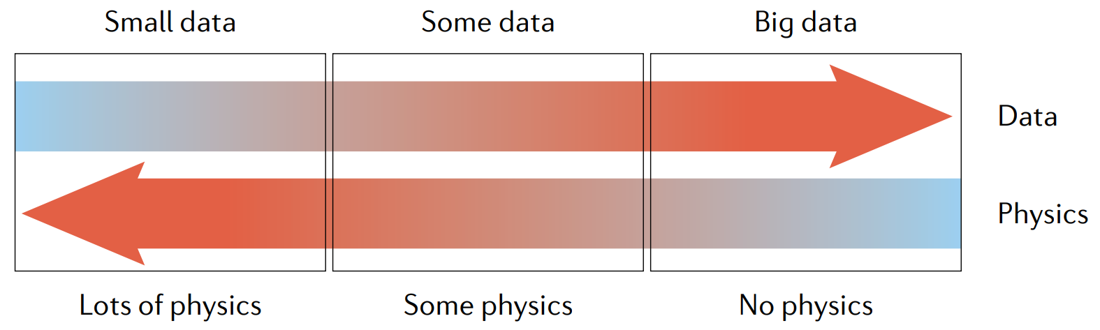
Figure 1: Three possible categories of physical problems and associated available data and knowledge of physics (Figure from [5]).

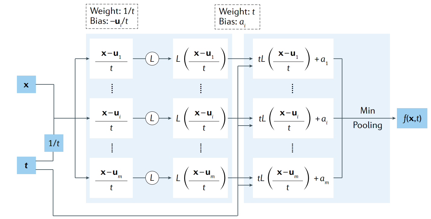
Figure 2: A neural network with the Lax–Oleinik formula baked into the architecture. Here, $f$ represents the solution of the Hamilton–Jacobi partial differential equations, while $x$ and $t$ correspond to the spatial and temporal variables, respectively. The activation function $L$ is convex and Lipschitz. The parameters $a_{i}\in\mathbb{R}$ and $u_{i}\in\mathbb{R^{n}}$ are specific to the neural network. Image courtesy of J. Darbon and T. Meng, Brown University and cited here from [5].

While existing work mainly focuses on isolated physical phenomena [7, 8, 9], and lacks the generalization of the approaches to wider problems, we propose Physics Encoded Residual Neural Network (PERNN), a general framework to capture complex behaviour of real-world systems. Our approach aims to target scenarios where data availability from the target systems is limited to specific operating scenarios and known physics only captures specific regions of the behaviour. Our approach defines a hybrid neural network which comprises feature extraction blocks to compute unknown variables (learning blocks) and combines them with differentiable physics operator layers (physics blocks) to model the complete behaviour of the target system. To facilitate the convergence of the model, we introduce intermediate ‘residual’ layers between the physics and the learning blocks. We also make our code available publicly on GitHub.

In this way, domain knowledge can inform the underlying neural network architecture while the gradient descent optimization using data can fill in gaps [11, 12]. The goal is to leverage interpretable mechanistic modelling to improve generalization and avoid relying solely on empirical correlations [13, 14]. This approach could benefit several complex systems, including robotic platforms [15, 16], autonomous vehicles [17], and aircraft swarms [18].

In this paper, we present two concrete applications to evaluate our method. The first application is based on simulating two-degrees of freedom for a robotic motion as it navigates across specified trajectories. For this, we extend on the work by Lutter et al. where they propose a deep neural network encoding Lagrangian Mechanics (DeLaN) to model the equations of motion for the robotic motion [19]. We formulate their architecture in the context of ’knowledge blocks’ and add residual layers to enhance the learning. For the second application, we test our approach on a more complex real-world problem where we model the behaviour of dynamic steering for autonomous grounded vehicles using a hybrid neural network architecture with the same concept of knowledge blocks. The well-established pure pursuit algorithm provides a physics-derived steering model accounting for dynamics like turn radius. Our architecture includes blocks of fully connected layers to discover intermediate unknown variables in the driving environment. It combines them with differentiable geometrical and kinematic operators from the pure pursuit model. We train this hybrid model observation data from an existing expert driving system inside a simulation environment. The goal is to learn the expert driver’s behaviour or policy using supervised learning. This forms a Behaviour Cloning problem, which involves transforming an expert’s demonstrations into i.i.d state-action pairs and learning to imitate the expert actions given each recorded state using a policy function. In the context of digital twins specifically, this approach is helpful since the underlying goal is to model the exact behaviour of a real-world system using observation data.

This paper presents the following key contributions of our work:

• It is the first (to our understanding) generic framework for embedding physics models into neural networks for end-to-end training on observation data.

• It is a significantly more interpretable hybrid neural network comprising learning blocks predicting human-understandable variables and physics blocks predicting the actual target variables.

• It allows the implicit discovery of unknown environmental variables that are not measured or observed.

• It outperforms the current state-of-the-art Physics Informed Machine Learning model for the Lagrangian-based robotic motion model in terms of accuracy of predicted torque and forces of motion.

• It outperforms conventional neural networks regarding key driving metrics on unseen road scenarios inside the simulation environment.

• It uses significantly fewer observation data, with fewer parameters, than conventional neural networks while outperforming key driving metrics inside the simulation environment.

2 Related Work

Physics Informed Machine Learning (PIML) is a recent approach that combines prior physics knowledge with conventional machine learning approaches to form hybrid learning algorithms of processes. Approaches like Physics-Informed Neural Networks (PINNs) encode analytical equations as loss terms to constrain deep learning models. Making a learning algorithm physics-informed refers to applying appropriate observational, inductive, or learning biases that direct the learning process towards identifying physically consistent solutions [5].

Several methods have been proposed to incorporate observational bias in the form of input data generated from variable fidelity physical systems as a weak form of prior knowledge [5, 20, 21]. However, abundant data must be available, especially for large deep-learning models, making scaling these approaches to other areas difficult. Another approach to PIML involves incorporating a learning bias into the learning model by penalizing the cost function of deep learning algorithms regarding adherence to a physical constraint, such as satisfying a partial differential equation (PDE) associated with the modelled process. In this way, the learning model attempts to fit both the observational data and the constraining equation or rule, for example, conservation of momentum and mass [22, 23, 24, 25, 26]. This, however, only adds a soft constraint to the learning model as the physics no longer plays a direct, explicit role after the training of the model is complete. A more direct approach to PIML is incorporating an inductive bias into the learning model through crafted architectures of neural networks (NNs) to embed prior knowledge and constraints related to the given task, such as symmetry and translation invariance. For differential equations in particular, several approaches have been investigated to modify NN architectures to satisfy boundary conditions or encode a priori parts of PDE solutions [27, 28, 29, 30, 31]. However, these models can struggle with extremely complex emergent behaviours arising from unknown dynamics outside the scope of hand-coded physics [32].

Differentiable physics-based PIML methods are based on incorporating inductive biases into the neural network architectures. This has allowed the integration of physical simulators directly into deep learning architectures through automatic differentiation [33, 34]. But most of these applications have focused on modelling isolated phenomena rather than full-system behaviours and provide particular architectures suited to only the respective problem spaces [7, 8, 9]. A generic framework for integrating physics models into learning-based data-driven models remains an open challenge. Furthermore, applying these methods in digital twin scenarios where the observational data and prior knowledge are limited and only partially known is restrictive and requires thorough exploration. The method defined in this paper herewith effectively addresses these issues.

3 Knowledge Blocks with Residual Learning

To address the problem of learning the behaviour of a target system with limited observation data and partially known physics, we propose a novel approach to integrate physics models into traditional neural networks to form modular architectures with ‘knowledge blocks’. These blocks are of two categories:

1. Physics blocks: representations of known physics equations as computational graphs comprising non-trainable parameters and static operators to reflect the mathematical operations of the equations.

2. Learning blocks: conventional neural network layers comprising trainable parameters (weights).

The physics blocks provide an a priori understanding of the system’s fundamental behaviour. The learning blocks can learn unknown, intermediate variables in the input space required by the physics blocks to predict the target variable(s). Collectively, the connected blocks form a neural network that can be trained end to end on observation data generated by the target system. For the scope of this work, we assume that the physics block encoding the known physics equation(s) of the target system can be represented as a differentiable physics model. This is necessary to define the physics equation(s) as a computational graph that can be integrated with the conventional learnable layers of a neural network.

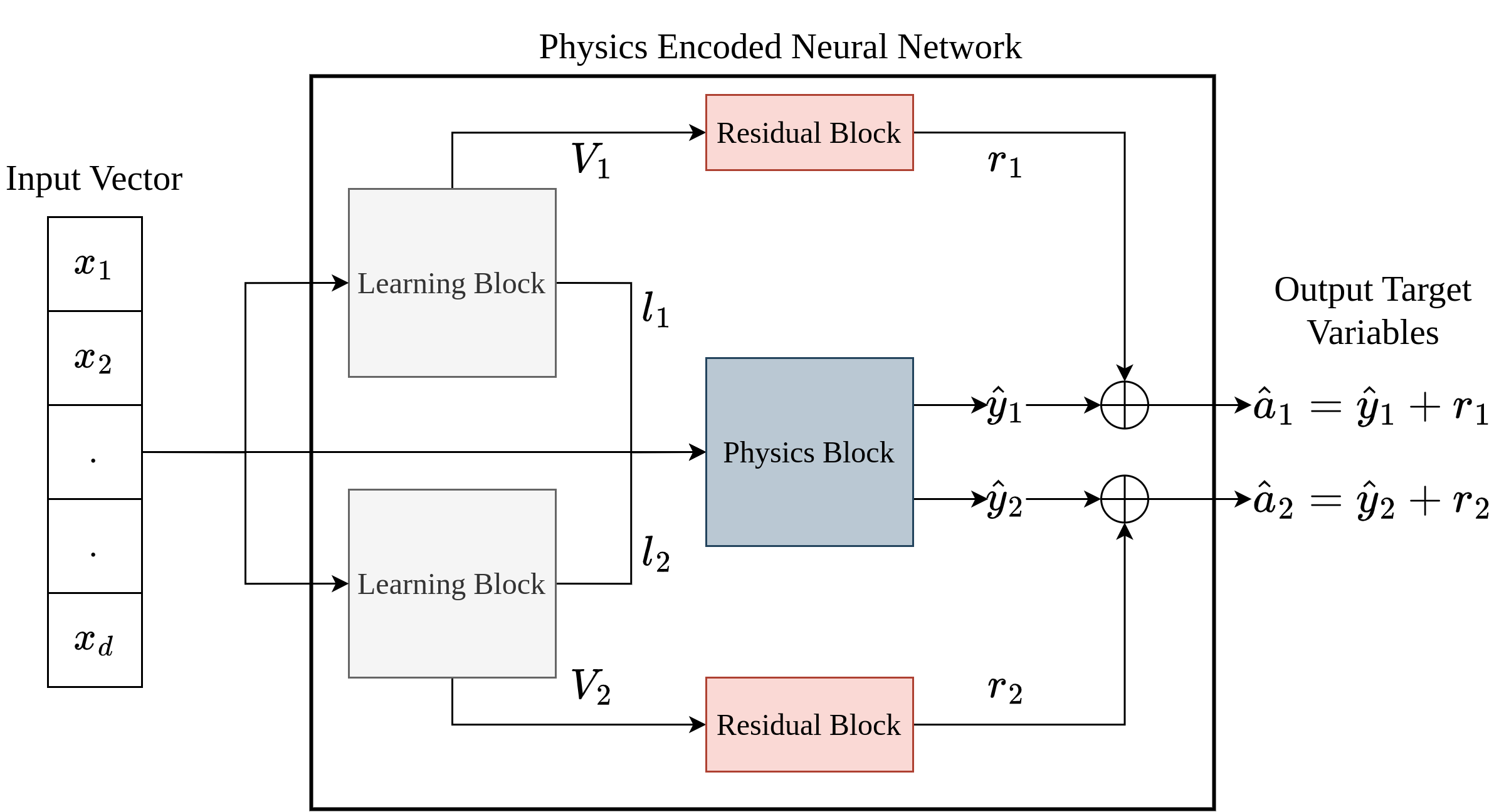
Figure 3: Proposed Physics-Encoded Neural Network Architecture with Residual Blocks. The example shows a problem case with two target intermediate variables and two target values to be predicted. Intermediate, unknown variables $l_{1}$ and $l_{2}$ are predicted (discovered) by the learning blocks and passed to the physics block as inputs alongside the original input vector $X$. Intermediate feature vectors $V_{1}$ and $V_{2}$ are passed from the learning blocks to the residual blocks to predict residual target values $r_{1}$ and $r_{2}$. The residuals eventually add up with the physics-predicted target values $y_{1}$ and $y_{2}$ to output the final target values $a_{1}$ and $a_{2}$.

To explain the proposed architecture, we define a Behaviour Cloning problem where expert demonstrations from the target system are used to learn a policy to model observed states (inputs) to actions (target values) taken. For a set of expert demonstrations $T$ from the target system, we assume i.i.d state-action pairs as:

$$T=\{(\textbf{x}_{1},a_{1}),(\textbf{x}_{2},a_{2})...(\textbf{x}_{n},a_{n})\}$$

We define a learning block as a set of fully connected layers $\mathcal{L}(\textbf{x};\theta)$ that takes observed state vector x and outputs an intermediate state vector l. The learning block has a set of trainable weights $\phi$.

$$\textbf{l}=\mathcal{L}(\textbf{x};\phi)$$

This intermediate state could include unknown variables from the environment or parts of the behaviour that are not directly defined by prior physics and thereby require empirical modelling. We also define our physics block as a computational graph $\mathcal{P}$ that predicts an action $a\in\mathcal{A}$, from the available set of actions $\mathcal{A}$ usually taken by the target system, using the observed state $x$ and the intermediate state l:

$$\hat{a}=\mathcal{P}(\textbf{x},\textbf{l})$$

We can then define our policy function $\pi$ to predict optimal action given the current state:

$$\hat{a}=\pi(\textbf{x},\mathcal{L},\mathcal{P})\text{ where }\hat{a}\in\mathcal{A}$$

Residual Learning in Knowledge Blocks

While the physics blocks provide key a priori knowledge to the model, they pose a significant problem in converging the loss function in the gradient descent algorithm. If the fixed relationships defined by these layers conflict with the learning blocks’ modelled patterns, it can result in conflicting gradients. This can make the training process highly unstable, thereby affecting convergence. Furthermore, static layers, such as those representing fixed physics equations, do not have learnable parameters or tweakable weights. When these static layers are integrated into a neural network, they can disrupt the flow of gradients to the learnable layers, often exacerbating the known problems of vanishing and exploding gradients.

To overcome this problem, we propose to add ‘residual blocks’ (similar to the concept introduced in the original ResNet paper [10]) that branch out from the learning blocks to predict residual target value to be added to the physics block output. This introduces alternative pathways for gradients to flow to the learning blocks, mitigating the effect of the static layers within the physics blocks. Figure 3 shows an example case with two target intermediate variables and two target values to be predicted by the model. Intermediate, unknown variables $l_{1}$ and $l_{2}$ are predicted (discovered) by the learning blocks and passed to the physics block as inputs alongside the original input vector $X$. Intermediate feature vectors $V_{1}$ and $V_{2}$ are passed from the learning blocks to the residual blocks to predict residual target values $r_{1}$ and $r_{2}$. The residuals eventually add up with the physics-predicted target values $y_{1}$ and $y_{2}$ to output the final target values $a_{1}$ and $a_{2}$.

Consequently, we can update the following in our earlier example of a Behavioral Cloning problem. An intermediate layer output vector $V$ from the learning block $\mathcal{L}$ will be passed to a separate residual block $\mathcal{R}$, which also comprises trainable parameters $\phi_{r}$.

$$r=\mathcal{R}(V;\phi_{r})$$

The residual target value $r$ will then be added to the output from the physics blocks to predict the action $\hat{a}$.

$$\hat{a}=\mathcal{P}(\textbf{x},\textbf{l})+\textbf{r}$$

Thereby, the final policy function to the Behaviour Cloning problem will become:

$$\hat{a}=\pi(\textbf{x},\mathcal{L},\mathcal{P},\mathcal{R})\text{ where }\hat{a}\in\mathcal{A}$$

The gradient descent algorithm optimises any suitable loss function $L(a,\hat{a})$ that defines the difference between $a$ and $\hat{a}$. Since the policy function is differentiable and comprises the affine connection of $\mathcal{L}$ and $\mathcal{P}$, the gradients from $\nabla{L}$ will flow through the chain of static operators from the physics block $\mathcal{P}$ to optimize the weights in the learning block $\mathcal{L}$, thereby modulating the learning of intermediate unknown variables using known physical constraints of the system. This essentially gives the final model the capacity to learn unknown, empirical relationships in data while maintaining the fundamental structure of the physics of the behaviour being modelled.

4 Experimentation

We validate the effectiveness of our approach in two different experimental setups. The first involves modelling the dynamics of robotic motion using Lagrangian Mechanics (Euler-Lagrange equation) as the Physics Model in our physics-encoded architecture defined earlier. The second setup involves modelling steering dynamics for autonomous vehicle simulation. Here, we investigate the effectiveness of our approach in a more complex digital twin problem where prior physics only partially defines the system’s dynamics.

4.1 Learning Lagrangian Mechanics for Robotic Motion Simulation

We first investigate the effectiveness of our approach, especially the residual architecture’s effect, on a Lagrangian mechanics problem. In this section, we propose to learn the dynamics of robotic motion using the Euler-Lagrange differential equation from Lagrangian mechanics as prior physics knowledge for a learning model. We build on the Deep Lagrangian Networks (DeLaN) by Lutter et al. [19] and extend their architecture in the context of our framework using knowledge blocks. While the authors of DeLaN propose a framework very similar to ours, its applicability is restricted to Lagrangian Mechanics, not addressing the challenges associated with generalizability such as restrictions to gradient flow due to physics-based operators in the neural architecture. To address this, we propose to extend DeLaN architecture with a residual block and present the effectiveness of our framework.

DeLaN incorporates non-conservative forces, generalized coordinates q and generalized velocities $\dot{\textbf{q}}$ , which are the time derivatives of q. Generalized coordinates q refer to coordinates which uniquely identify the configuration of the system being modelled. DeLaN defines the Lagrangian, $L$ as a function of q and $\dot{\textbf{q}}$, as:

$$L(\textbf{q},\dot{\textbf{q}})=T(\textbf{q},\dot{\textbf{q}})-V(\textbf{q})$$

where $T$ is the kinetic energy and $V$ is the potential energy of the system. For systems undergoing rigid body motion, the kinetic energy can be calculated as the $T=\frac{1}{2}\dot{\textbf{q}}^{\top}\textbf{H}(\textbf{q})\dot{\textbf{q}}$, where $H(\textbf{q})$ is the mass matrix, which is symmetric and positive definite. The Euler-Lagrange equations of motion are given by:

$$\frac{d}{dt}\frac{\partial{L}}{\partial{\dot{\textbf{q}}}}-\frac{\partial{L}}{\partial{\textbf{q}}}=\tau$$

Hence the Lagrangian equations of motion becomes:

$$\textbf{H}(\textbf{q})\ddot{\textbf{q}}+\underbrace{\dot{\textbf{H}}(\textbf{q})\dot{\textbf{q}}-\frac{1}{2}(\frac{\partial}{\partial{\textbf{q}}}(\dot{\textbf{q}}^{\top}\textbf{H}(\textbf{q})\dot{\textbf{q}}))^{\top}}_{\textbf{c}(\textbf{q},\dot{\textbf{q}})}+\textbf{g}(\textbf{q})=\tau$$ (1)

Here, $\textbf{g}(\textbf{q})=dV/d\textbf{q}$ and $\textbf{c}(\textbf{q},\dot{\textbf{q}})$ describes the Centripetal and Coriolis forces. DeLaN approximates the inverse model by representing the unknown functions $g(\textbf{q})$ and $\textbf{H}(\textbf{q})$ as feed-forward networks (or single network with two output heads). Rather than representing $\textbf{H}(\textbf{q})$ directly, the lower-triangular matrix $\textbf{L}(\textbf{q})$ is predicted and used to calculate $\textbf{H}(\textbf{q})=\textbf{L}(\textbf{q})^{\top}\textbf{L}(\textbf{q})$. Therefore, DeLaN approximates the inverse model using two learned variables $\textbf{g}(\textbf{q},\theta)$ and $\textbf{L}(\textbf{q},\theta)$ where $\theta$ is the learnable set of weights for the feed-forward network. These variables are then fed to the operators in the Euler-Lagrange equation 1 to predict the motor torque $\hat{\tau}$. Further details of the formulation of these equations and the neural network structure behind DeLaN can be found in the original paper [19] and therefore not expanded upon in this paper.

4.1.1 Deep Lagrangian ‘Residual’ Network

We can reformulate the basic architecture behind DeLaN as a combination of knowledge blocks. Since the physics and learning blocks can be conceptually viewed as part of the original DeLaN architecture, we extend the architecture by adding a residual block. Figure 4 illustrates the original architecture from [19] as a combination of learning, residual and physics blocks. The feed-forward layers predicting $\textbf{g}(\textbf{q},\theta)$ and $\textbf{L}(\textbf{q},\theta)$ are illustrated as a learning block that output these intermediate variables into the physics block representing the Euler-Lagrange operators. In the figure, L is divided into off-diagonal ($l_{o}$) and diagonal ($l_{d}$) outputs from two different heads to guarantee positive definiteness. The theoretical understanding behind it can be found in the original paper [19]. The residual block takes as input one of the intermediate layer outputs from the learning block and outputs the residual value $r$. This residual value is added to the motor torque $\tau$ output from the physics block to form the final predicted motor torque value $\hat{\tau}_{target}$.

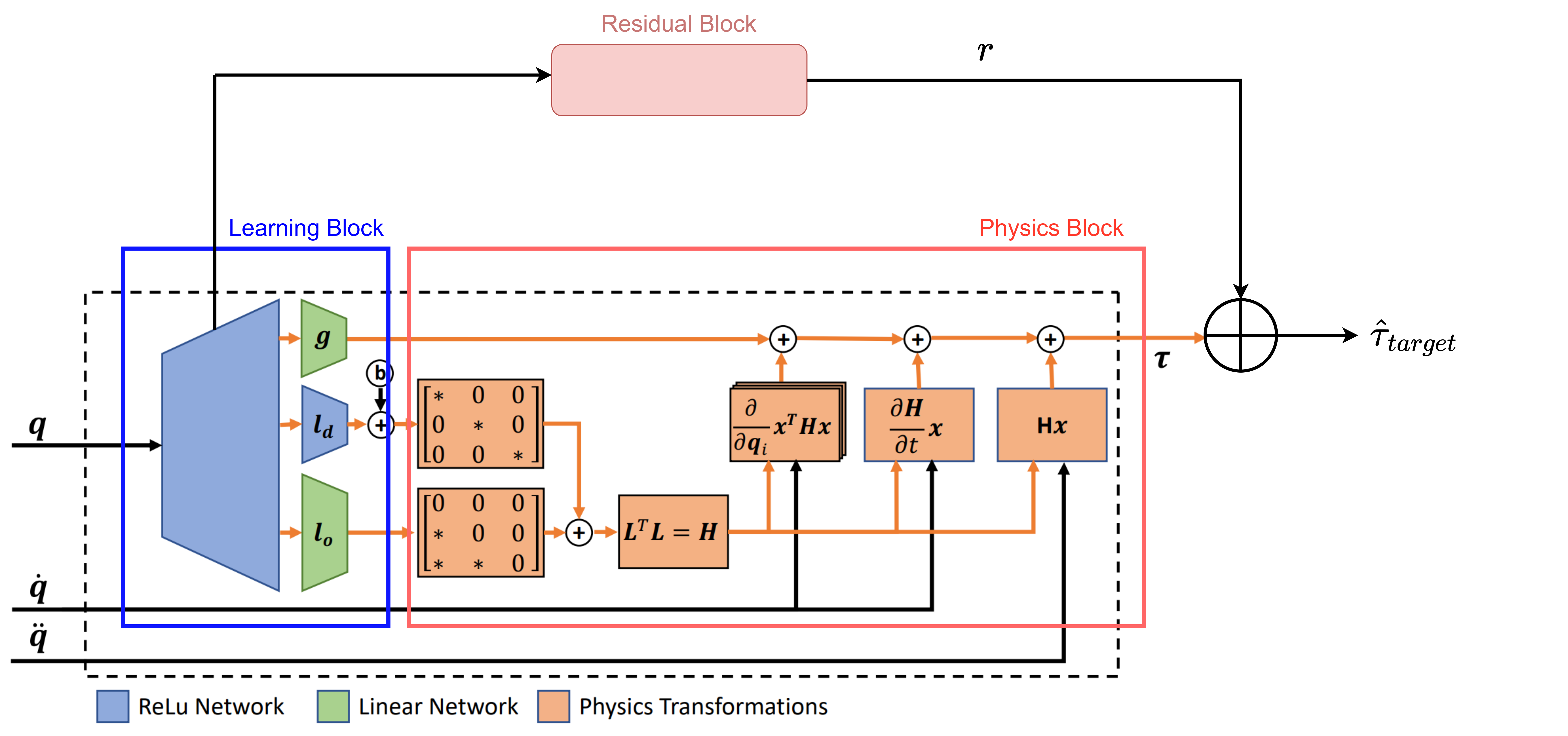
Figure 4: The computational graph from DeLaN [19] reformulated with learning, residual and physics blocks. The learning block (blue) comprises three separate heads to output g, $l_{o}$ and $l_{d}$. The physics block (orange) represents the mathematical operators from the Euler Lagrange equation. The residual block comprises a set of fully-connected layers, that use an intermediate layer output from the learning block as input. It predicts the residual value $r$ which is added to the predicted torque from the phyics block to output the final torque value $\hat{\tau}_{target}$

The complete computational graph forms our physics-encoded neural network that is trained end-to-end similar to the original DeLaN. The loss function is based on MSE (Mean Squared Error), minimizing the error between the observed ($\tau$ ) and predicted ($\hat{\tau}$) torque values. This is defined as:

$$L=\frac{1}{n}\sum_{i=1}^{D}(\tau_{i}-\hat{\tau}_{i})^{2}$$

We use the Mini-Batch Gradient Descent algorithm and Adam Optimizer to optimize the loss function, where $n$ is any arbitrary batch size for each sample in the gradient descent algorithm. The gradients for the learnable weights $\theta$ are calculated by the chain of function derivatives that involve the operators from the Euler-Lagrange equation, effectively guiding the learning to follow the physical constraints of the system. The residual blocks facilitate the learning process by providing alternate gradient pathways.

4.2 Steering Dynamics for Autonomous Vehicle Simulation

We now apply this framework to a more complex digital twin problem where the available data and prior physics may not be substantially available to completely model the system dynamics independently. We investigate our approach in an autonomous driving task of steering a vehicle in a simulation as it manoeuvres around a race track. Using data generated from an existing driving agent within the simulation (treated as a reference agent), we train a feed-forward neural network architecture that combines fully connected layers that capture perceptual understanding with relevant mathematical operators from the physics-based steering model known as Pure Pursuit. Figure 8 illustrates the proposed architecture and is explained in detail in section 4.2.2.

We use the TORCS open-source driving simulator as our experimental environment due to the tracks’ diversity and rich non-visual sensory and perceptual information [40]. The input parameter space offered to the model consists of a vehicle’s state variables and perception information from the surrounding environment. Table 1 summarizes the subset of the available variables from the simulation environment used as input parameters and actuators/actions for our model.

The vector of 19 range finder sensors ($R$) comprises the distance between the track edge and the car centre within a range of 200 meters. Each value represents clockwise distances from 0 to 180 degrees to the car axis at 10-degree intervals. This is similar to how an automotive RADAR sensor is used to localize objects in the long-range vicinity of the autonomous vehicle. Figure 5 illustrates this sensor setup. The same methodology defines the distances to surrounding traffic vehicles to define vector $O$, as Table 1 explains.

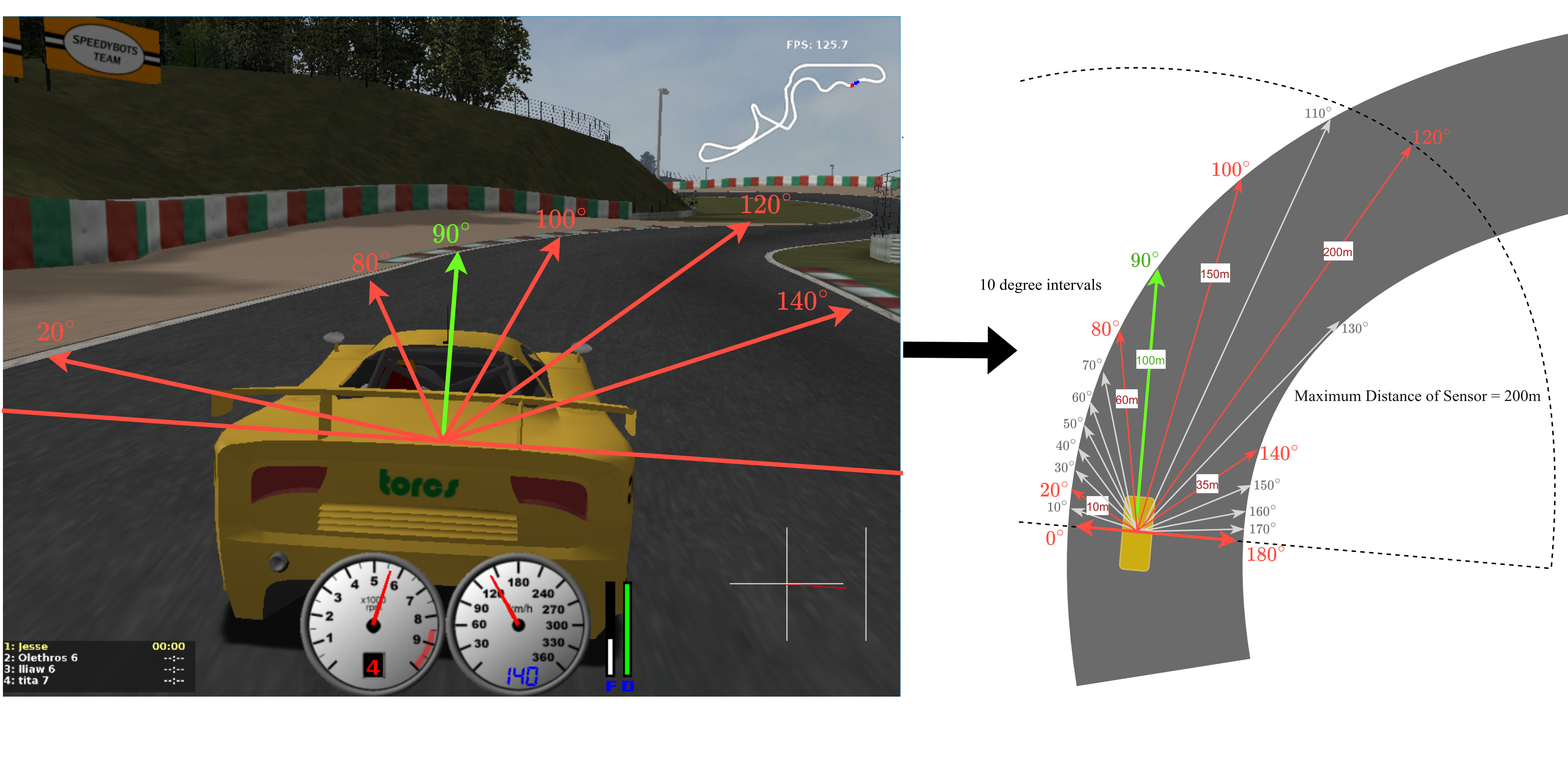
Figure 5: Illustration of the 19 range finder sensors ($R$) comprising distances to track edges, spanning clockwise from 0 to 180 degrees to the car axis at 10-degree intervals. The image from the TORCS simulation on the left shows a sample of sensors at different angles depicted with red arrows, which is further elaborated on in the figure on the right side. The maximum range of the sensors is 200m. A similar sensor setup defines distances to surrounding traffic vehicles ($O$).

Table 1: System and Actuator Variables in the Driving Environment

(a) State Variables

Variable	Range (unit)	Description
$\alpha_{axis}$	$[-\pi,+\pi]$ (rad)	Angle between the car direction and the direction of the track axis
$D_{center}$	$(-\infty,+\infty)$ (m)	Distance between the car and the track axis. The value is normalized w.r.t to the track width: it is 0 when the car is on the axis, -1 when the car is on the right edge of the track and +1 when it is on the left edge of the car
$z$	$[-\infty,+\infty]$ (m)	Distance of the car mass centre from the surface of the track along the $z$ axis
$V_{x,y,z}$	$(-\infty,+\infty)$ (km/h)	Speed of the car as a vector in $\mathbb{R}^{3}$
$R$	$[0-200]$ (m)	Vector of 19 range finder sensors: each sensor returns the distance between the track edge and the car within a range of 200 meters. By default, the sensors sample the space in front of the car every 10 degrees, clockwise from -90 to +90 degrees to the car axis.
$O$	$[0-200]$ (m)	Vector of 19 range finder sensors for traffic vehicles: each sensor returns the distance between a detected traffic vehicle and the subject car within a range of 200 meters. By default, the sensors sample the space in front of the car every 10 degrees, clockwise from -90 to +90 degrees to the car axis.

(b) Actuator Variables

Variable	Range (unit)	Description
$\delta$	$[-1,+1]$	Steering value: -1 and +1 represent right and left bounds, which corresponds to an angle of 0.366519 rad
$a$	$[0,1]$	Virtual acceleration pedal (0 means no gas, 1 full gas)
$b$	$[0,1]$	Virtual braking pedal (0 means no brake, 1 full brake)

4.2.1 Physics-based Pure Pursuit Steering Model

The pure pursuit algorithm is a path-tracking algorithm that steers a vehicle along a desired path, given a set of reference points to follow. The algorithm calculates the steering angle required to follow the path based on the vehicle’s current position and velocity [6]. It operates based on the concept of ”pursuit,” where a hypothetical point, known as the look-ahead point, is established ahead of the vehicle on the desired path. The objective is to steer the vehicle towards this point, thereby ensuring path tracking. The algorithm computes the optimal steering angle required to reach the look-ahead point by analyzing the geometric relationship between the vehicle and the path.

Firstly, the algorithm estimates the position of the look-ahead point by projecting it along the desired path based on the vehicle’s current position. Subsequently, the algorithm computes the curvature of the path at the look-ahead point using mathematical techniques such as interpolation or curve fitting. Finally, utilizing the vehicle’s kinematic model, the algorithm calculates the required steering angle to navigate towards the look-ahead point. The look-ahead distance is a control parameter in the context of the algorithm and affects the outcome in two contexts: 1) Regaining a path, i.e., the vehicle is at a “large” distance from the path and must attain the path. 2) Maintaining the path, i.e., the vehicle is on the path and wants to remain on the path. The effects of changing the parameter in the first problem are easy to imagine using the analogy to human driving. The longer look-ahead distances converge to the path more gradually and with less oscillation, as illustrated in Figure 6. It, therefore, depends on the state of the driving environment at any point in time to optimally set the look-ahead distance to manoeuvre the track safely.

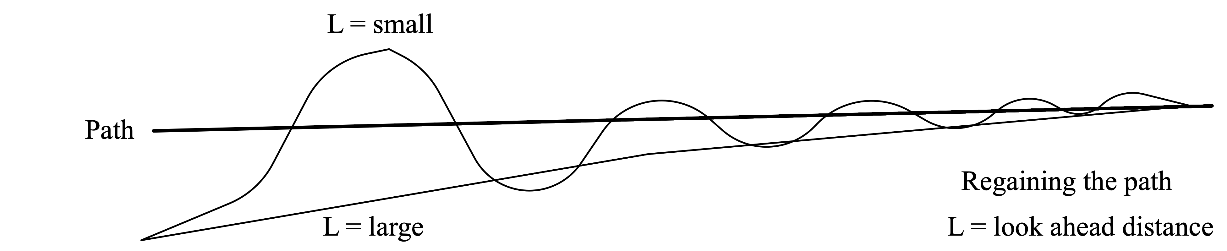
Figure 6: The effect of look-ahead distance magnitude on the behaviour of path convergence [41]

The Pure Pursuit model defines a reference point on the road as a vector of two observed scalar values: the heading difference (angle) to the direction of the reference point and the lookahead distance to the reference point. Formally, this can be represented as:

z $$=\begin{bmatrix}l\\ \theta_{target}\end{bmatrix}$$

where z is the reference point, and $l$ and $\theta_{target}$ are the lookahead distance and heading difference accordingly. We assume that the vehicle follows the principle of a rigid body moving around a circle and, therefore, compute the required steering angle using this circle’s instantaneous centre of rotation. Figure 7 illustrates this concept. Consequently, from the arc of rotation depicted in the figure, we can use the law of sine to calculate the curvature, $k$, of the path to the selected point as:

$$\frac{l}{\sin{2\theta}}=\frac{r}{\sin(\frac{\pi}{2}-\theta)}$$

$$\frac{l}{\sin\theta\cos\theta}=\frac{r}{\cos\theta}$$

$$\frac{l}{\sin\theta}=2r$$

$$k=\frac{1}{r}=\frac{2\sin\theta}{l}$$ (2)

Here, $r$ is the radius of rotation for the vehicle. Furthermore, we know from the kinematic bicycle model that the radius of rotation has an inverse relationship with the steering vehicle as:

$$r=L/\tan(\delta)$$

Here, $\delta$ is the steering angle and $L$ is the wheelbase of the vehicle (horizontal distance between rear and front wheel centers). Therefore, we can substitute $r$ from the equation of curvature (Equation 2) to get the required steering angle as:

$$\delta=\arctan(\frac{2L\sin\theta}{l})$$ (3)

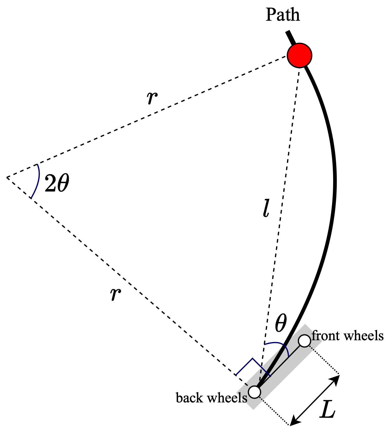
Figure 7: Geometric relationship between the circle of rotation, wheelbase of the vehicle ($L$), lookahead distance ($l$), and the heading difference ($\theta$).

4.2.2 Physics Encoded Residual Feed-Forward Network

Based on the approach introduced in section 3, we formulate our physics block as the mathematical operations calculating the target steering angle within the Pure Pursuit algorithm. As previously discussed in section 4.2.1, the selected reference point and look-ahead distance are key parameters that dictate the steering behaviour and are based on the geometry of the driving path ahead. Consequently, we formulate our learning block as a set of fully connected layers to output the optimal look-ahead distance $l$ and heading difference $\theta_{target}$ to represent the selected reference point z on the road to follow (see Equation 4.2.1). It is important to note that these variables are unknown in the input space (sensor information) and are thereby ‘discovered’ by the learning blocks.

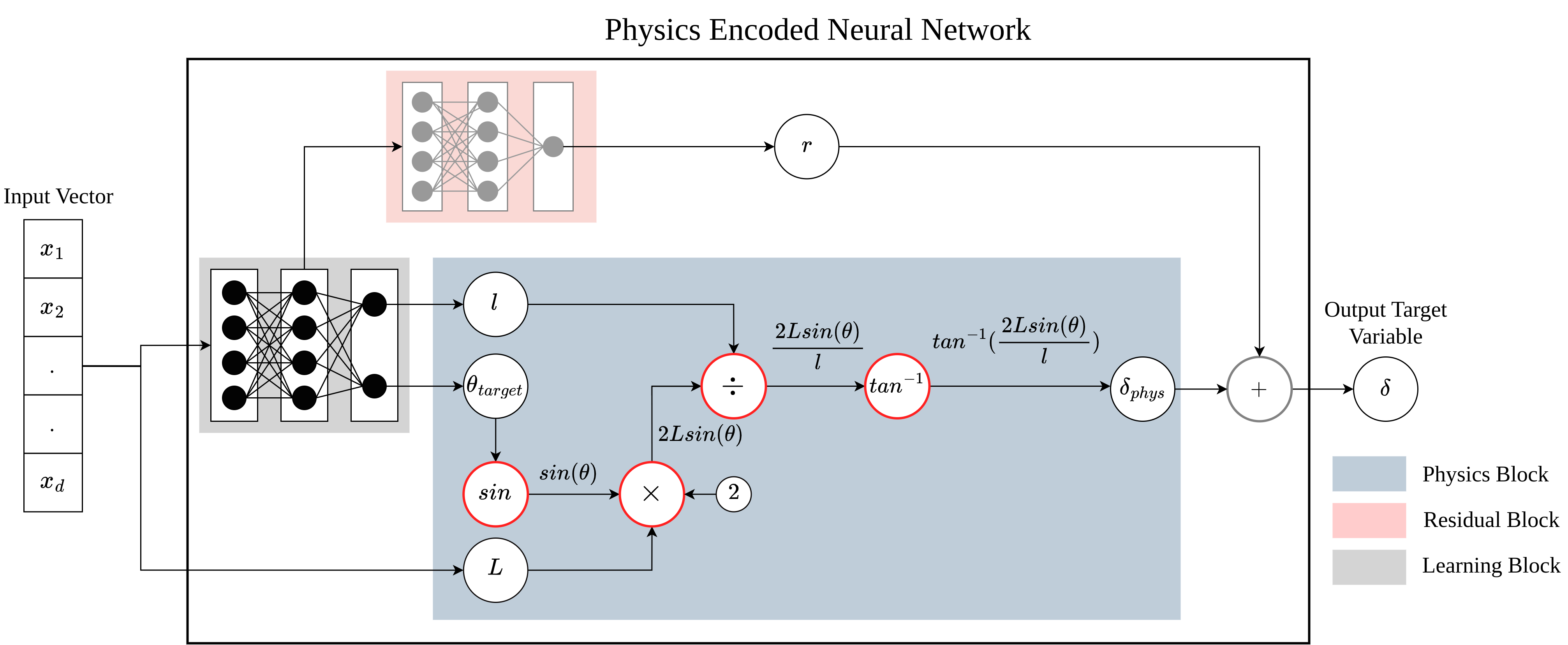
Figure 8: Physics Encoded Neural Network architecture for the steering model. The learning block predicts two unknown variables from the input space: $l$ (lookahead distance) and $\theta_{target}$ (heading difference to selected reference point). These variables are passed as input to the physics block to predict the steering angle $\delta$. The intermediate layer output from the learning block is passed to the residual block to predict the residual value to be added to $\delta$ for the final steering value

Algorithm 1 Two-Phased Behavior Cloning Using Physics-Encoded Neural Network

1:Input: Demonstration Data 1 ($\mathcal{D}_{1}$), Demonstration Data 2 ($\mathcal{D}_{2}$), Loss Threshold ($\ell_{\text{thresh}}$)

2:Output: Integrated Model ($M$)

3:Initialize Integrated Model $M$ comprising three blocks $\mathcal{L}$, $\mathcal{R}$, $\mathcal{P}$

4:Initialize learning block $\mathcal{L}$ (learnable)

5:Initialize physics block $\mathcal{P}$ (non-learnable)

6:Initialize residual block $\mathcal{R}$ (learnable)

7:Initialize heuristic function $H$ for label generation

8:

9:Phase I: Warm Start - Train Block $\mathcal{L}$ with Heuristic Labels

10:repeat

11:     Sample mini-batch of state-action pairs from $\mathcal{D}_{1}$

12:     Generate labels using the heuristic function $H$

13:     Forward pass through block $\mathcal{L}$

14:     Compute loss ($\ell_{1}$) for predicted lookahead distance and target heading differences

15:     Backward pass and update the weights in block $\mathcal{L}$

16:until convergence

17:

18:Phase II: Train Complete Model $M$

19:Initialize block layers in $\mathcal{L}$ with weights from Phase I

20:repeat

21:     Sample mini-batch of state-action pairs from $\mathcal{D}_{2}$

22:     Forward pass through models $\mathcal{R}$ and $\mathcal{L}$ with static block $\mathcal{P}$

23:     Compute loss ($\ell_{2}$) for predicted steering

24:     Backward pass and update weights in blocks $\mathcal{R}$ and $\mathcal{L}$

25:until $\ell_{2}<\ell_{\text{thresh}}$

26:

27:return Trained model $M$

These variables are then fed to the physics block, a computational graph expressing the steering angle as a geometric combination of the lookahead distance and heading difference from the fully connected layers and the vehicle’s wheelbase (available in the input space). These include the operations in Equation 3 to calculate the target steering based on the input variables.

To formally define each block, let x be the vector of input parameters (explained in Table 1). Let us assume $\mathcal{L}(\textbf{x},\phi)$ represents the function modelled by the learning block predicting the lookahead distance $l$ and target heading difference $\theta_{target}$, with known input variables $x$ and a set of learnable weights $\phi_{learn}$.

$$\mathcal{L}:\mathbb{R}^{d}\times\mathbb{R}^{m}\rightarrow\mathbb{R}^{2}$$

$$\mathcal{L}(\textbf{x},\phi_{learn})=\begin{bmatrix}l\\ \theta_{target}\end{bmatrix}$$

where $d$ is the number of state features in the input vector (from available state parameters shown in Table 1), and $m$ is the total number of weights in the fully connected layers.

Let us also assume our physics block $\mathcal{P}(\textbf{x},\mathcal{L})$ to predict the steering value $\delta_{phys}$ using the known input state and the intermediate unknown variables predicted by $\mathcal{L}$, using operators from Equation 3.

$$\mathcal{P}(\textbf{x},\mathcal{L})=\arctan(\frac{2L\sin\theta}{\mathcal{L}(x)})$$

We also define a residual block $\mathcal{R}(V;\phi_{res})$ comprising a set of fully connected layers with learnable weights $\phi_{res}$, which inputs a feature vector from an intermediate layer from the learning block $\mathcal{L}$ as input. The residual block predicts the residual target value $r$, which is added to the physics-predicted steering value $\hat{\delta}_{phys}$ to formulate the final steering value from the model.

$$\hat{\delta}=\mathcal{P}(\textbf{x},\mathcal{L})+\textbf{r}$$

Based on the Behavior Cloning problem discussed in section 3, we can assume a set of demonstration data $T$ from an expert driving agent as i.i.d state-action pairs:

$$T=\{(\textbf{x}_{1},\delta_{1}),(\textbf{x}_{2},\delta_{2})...(\textbf{x}_{n},\delta_{n})\}$$

Here, $\textbf{x}_{i}$ and $\delta_{i}$ are observed input state and steering values from the expert driving agent. We can then define the predicted steering value (target value) based on the policy function $\pi$ as:

$$\hat{\delta}=\pi(\textbf{x},\mathcal{L},\mathcal{P})\text{ where }\hat{a}\in\mathcal{A}$$

The loss function is based on MAE (Mean Absolute Error), minimizing the error between the observed ($\delta$ ) and predicted ($\hat{\delta}$) steering angles. This is defined as:

$$L=\frac{1}{n}\sum_{i=1}^{D}|\delta_{i}-\hat{\delta}_{i}|$$

We use the Mini-Batch Gradient Descent algorithm and Adam Optimizer to optimize the loss function, where $n$ is any arbitrary batch size for each sample in the gradient descent algorithm. The gradients for the learnable weights in $\phi_{learn}$ are calculated by the chain of function derivatives that involve the geometric and kinematic operators from Equation 2. This allows our feed-forward network to learn the optimal lookahead while being forced to comply with the geometric and kinematic aspects of the steering problem dictated by the pure pursuit algorithm. This is done by constraining the calculation of gradients, which are calculated as an explicit part of the equations based on the pure pursuit algorithm. On the other hand, the residual block provides an alternative pathway for the gradients to flow back to the intermediate layers of the learning block. This allows the loss function to converge and optimise the weights in the residual and, more importantly, the learning block.

4.2.3 Training on Demonstration Data

We train our physics-encoded neural network model on the demonstration data $T$ in two sequential phases. The first phase involves a warm-start phase where the learning block is trained separately to predict appropriate lookahead distance ($l$) and target heading difference ($\theta$) values. We generate two batches of data from our simulation (details in section 5.2.1). The first batch is generated from the agent driving on empty segments of tracks, and the second batch is generated from the agent driving amongst other traffic vehicles. The sequence of steps in the training process is defined in Algorithm 1.

Phase I: Warm Start

In this phase, the learning block is trained separately on the first dataset ($\mathcal{D}_{1}$) collected from empty road scenarios. We define a heuristic function to provide the learning block with proposed values of lookahead distance ($l$) and target heading difference ($\theta_{target}$) for each data point. The heuristic function selects the reference point to be in the direction of the furthest point on the road boundary from the vehicle, using the range-finding sensor vector $R$ (refer to Table 1).

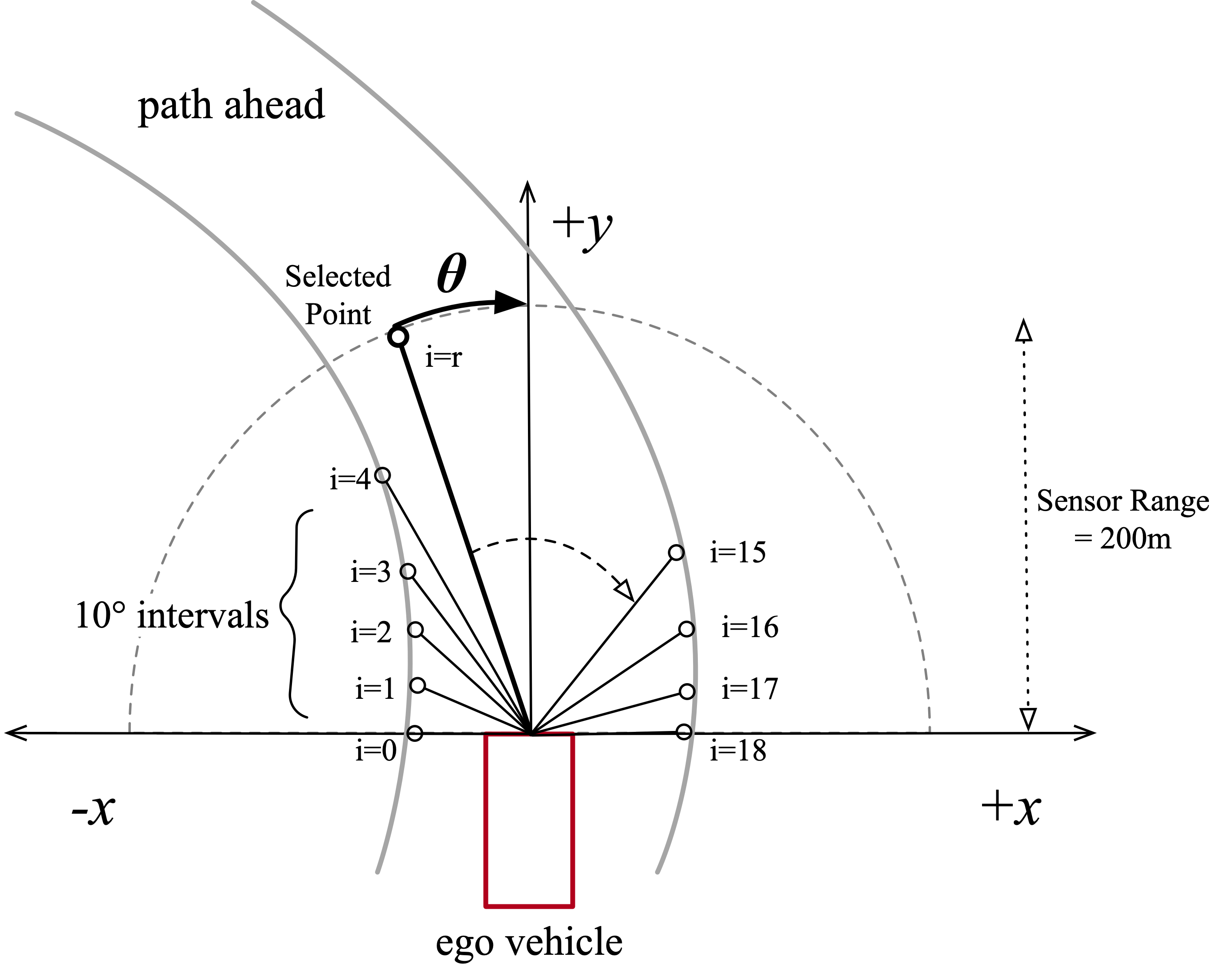
Figure 9: Proposed method to find the reference direction for vehicle, based on the maximum range finder sensor values

Figure 9 illustrates this method. The range finder sensors can be considered to run clockwise from the vehicle’s horizontal plane, from the left side of the vehicle, forming a semi-circle axis in front of the vehicle. The sensors capture values every 10 degrees on this axis, clipped to a maximum value of 200m. These values depict the presence of a road boundary at the corresponding angle value. Formally, for $R_{t}$ as the vector of range finder sensors from a data point $t$, we can define:

$$i=argmax(R_{t})$$

where $i$ is the index of the maximum distance value in vector $R_{t}$. If there are multiple maximum values, the index of the first of these values is picked. Using this index $i$, we can calculate $\theta_{t}$ (in degrees) and $l_{t}$, for any given data point $t$, as follows:

$$\theta_{t}=10i-90$$

$$l_{t}=R_{t}^{i}$$

We then use the output from the heuristic function to provide target labels for the learning block. The loss function is based on MAE (Mean Absolute Error), minimizing the error between the heuristic output and predicted values from the learning block. This is optimized using a simple Mini-Batch Gradient Descent with Adam Optimizer until an arbitrary point of convergence where the mean loss function value across mini-batches falls below a threshold.

Phase II: Train Complete Model

We refer to the complete model $M$ as the connected neural network with the learning ($\mathcal{L}$), learning ($\mathcal{R}$) and learning ($\mathcal{P}$) blocks, as shown in Figure 8. The learned weights from Phase I are used to initialize the learning block. We then train $M$ on the second dataset ($\mathcal{D}_{2}$) comprising traffic scenarios, with the observed steering values as target values from which the model can learn. The training is based on the explanation in section 4.2.2.

5 Results

In this section, we present experiments and analyses related to the two applications discussed in the last two sections. The first set of experiments related to robotic motion modelling will exhibit the specific improvements that the residual aspect of our approach presents, especially when combining physics and learning blocks in a single neural network architecture. The second set of experiments expands on the broader advantages of this method in achieving higher generalizability with less data and lower model complexity compared to other methods.

5.1 Robotic Motion Simulation

As a base evaluation, we compare our Physics Encoded Residual Neural Network (PERNN) approach to the DeLaN method for modelling Lagrangian dynamics in simulated robotic motion. We use the original experimental setup from [19] for simulated 2-dof robot and compare the effectiveness of our architecture against DeLaN. For experimental consistency, the architecture for the learning and physics blocks are kept constant for both approaches. This presents a fair analysis of the impact of the residual blocks in the optimization process. Since the original work on DeLaN proves the superiority of the base architecture against traditional methods such as feed-forward neural networks, we only compare the results of PERNN with DeLaN to showcase the improvements resulting from our contribution.

5.1.1 Data Generation

Figure 10 illustrates the experimental setup, as presented in [19]. The original work presented three experimental setups: a simulated 2-dof robot drawing the cosine trajectories, a simulated Barrett WAM drawing the 3d cosine 0 trajectory and finally, the physical 7-dof Barrett WAM robot. We limit the scope of experiments to only the simulated 2-dof robot. Here, the generalized coordinates and joint torques are used as input to simulate the character and cosine trajectories using- PyBullet simulation. Table 2 presents the experiment details. 17 unique character trajectories were used as a training set for both models, and the results were calculated and compared over three character trajectories. The training dataset $\mathcal{D}$ consists of state-action pairs as follows:

$$\mathcal{D}=\{((\textbf{q}_{1},\dot{\textbf{q}}_{1},\ddot{\textbf{q}}_{1}),\tau_{1}),((\textbf{q}_{2},\dot{\textbf{q}}_{2},\ddot{\textbf{q}}_{2}),\tau_{2}),...((\textbf{q}_{1},\dot{\textbf{q}}_{n},\ddot{\textbf{q}}_{n}),\tau_{n})\}$$

Here, q, $\dot{\textbf{q}}$ and $\ddot{\textbf{q}}$ are the generalized coordinates, velocities and acceleration values and $\tau$ is the corresponding motor torque for each instance in time of the simulated robotic joints.

Table 2: Details on the training and test data for modelling 2-dof robotic motion using DeLaN and PERNN methods

Train Samples	2459
Train Characters	[’b’, ’o’, ’l’, ’s’, ’u’, ’w’, ’y’, ’a’, ’z’, ’h’, ’m’, ’p’, ’c’, ’d’, ’r’, ’g’, ’n’]
Test Characters	[’e’, ’v’, ’q’]
Training Iterations (Epochs)	5000

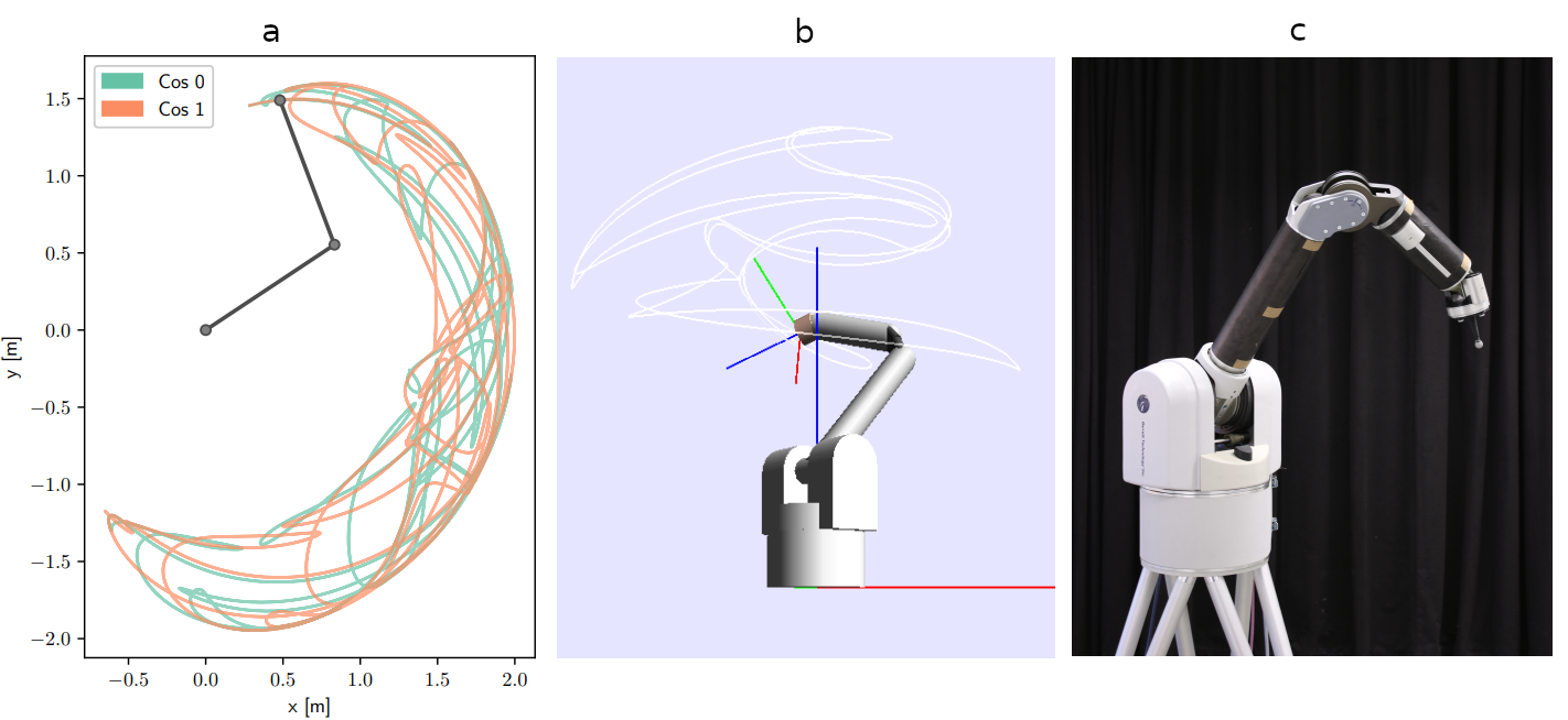
Figure 10: The experimental setup carried out by [19] (a) The simulated 2-dof robot drawing the character/alphabet trajectories. (b) The simulated Barrett WAM drawing the 3d cosine 0 trajectory. (c) The physical Barrett WAM. This paper presents experiments on (a), a simulated 2-dof robot drawing trajectories of characters/alphabets

5.1.2 Results

Figure 11 shows the ground truth torques of the test characters ‘e’, ‘v’ and ‘q’, the torque ground truth components and the learned decomposition using DeLaN and PERNN respectively. Even though both PERNN and DeLaN are trained on the super-imposed torques, they both learn to discern the inertial force $\textbf{H}(\ddot{\textbf{q}})$, the Coriolis and Centrifugal force $\textbf{c}(\textbf{q},\dot{\textbf{q}})$ and the gravitational force $\textbf{g}(\textbf{q})$. It can be seen that PERNN outperforms DeLaN in disambiguating the ground-truth torque values as well as these forces, as can be seen by the overlap between the ground-truth (black) and predicted (red) in the respective curves. Table 3 summarizes the Mean Squared Error values on the test character trajectories for the torque, inertial force $\textbf{H}(\ddot{\textbf{q}})$, the Coriolis and Centrifugal force $\textbf{c}(\textbf{q},\dot{\textbf{q}})$ and the gravitational force $\textbf{g}(\textbf{q})$ involved in the robotic motion. Note that the ground truth for the inertia and force values involved in the robotic motion can be measured from the PyBullet simulation and is therefore part of the available training data. However, the actual input to both models only comprises q, $\dot{\textbf{q}}$ and $\ddot{\textbf{q}}$ are the generalized coordinates, velocities and acceleration values.

The results illustrate the effectiveness of the residual blocks in our general Physics Encoded Neural Network framework in its capability to facilitate the optimization of loss functions when physics models are directly baked into neural architectures. In the next section, we evaluate our general framework on a complex, real-world problem.

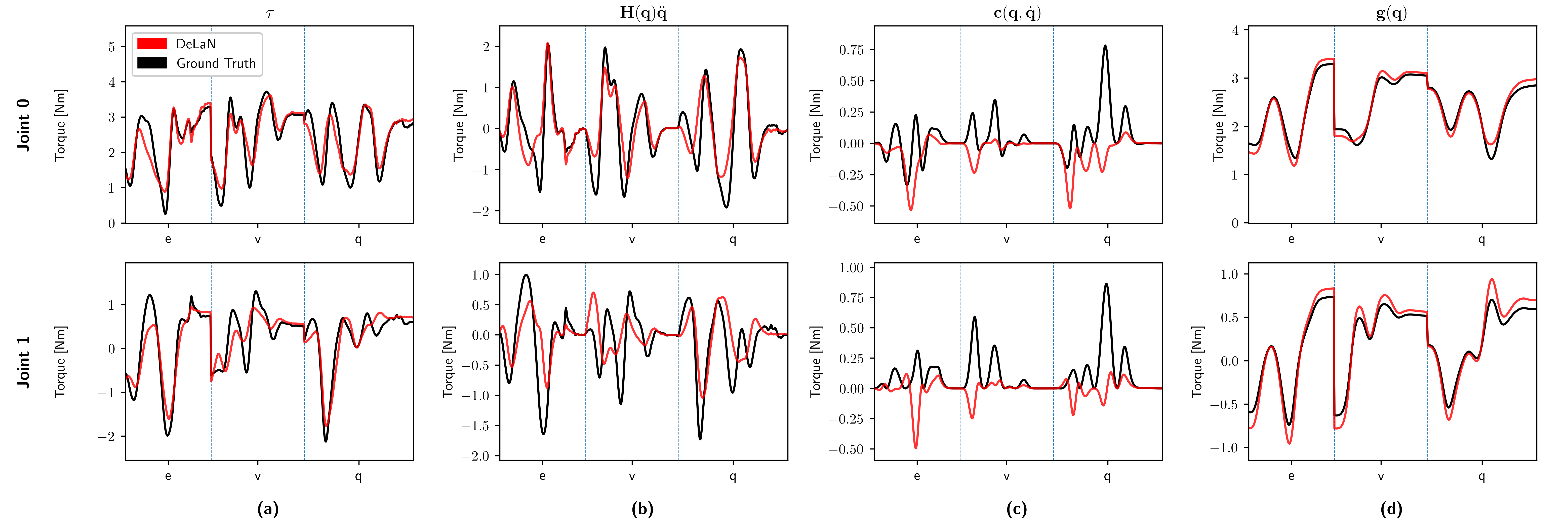
(a) The torque $\tau$ required to generate the characters ’e’, ’v’ and ’q’ in black. Using these samples DeLaN was trained offline and learns the red trajectory. Using Equation 1 DeLaN can represent the inertial force $\textbf{H}(\ddot{\textbf{q}})$, (b), the Coriolis and Centrifugal forces $\textbf{c}(\textbf{q},\dot{\textbf{q}})$ (c) and the gravitational force $\textbf{g}(\textbf{q})$ (d)

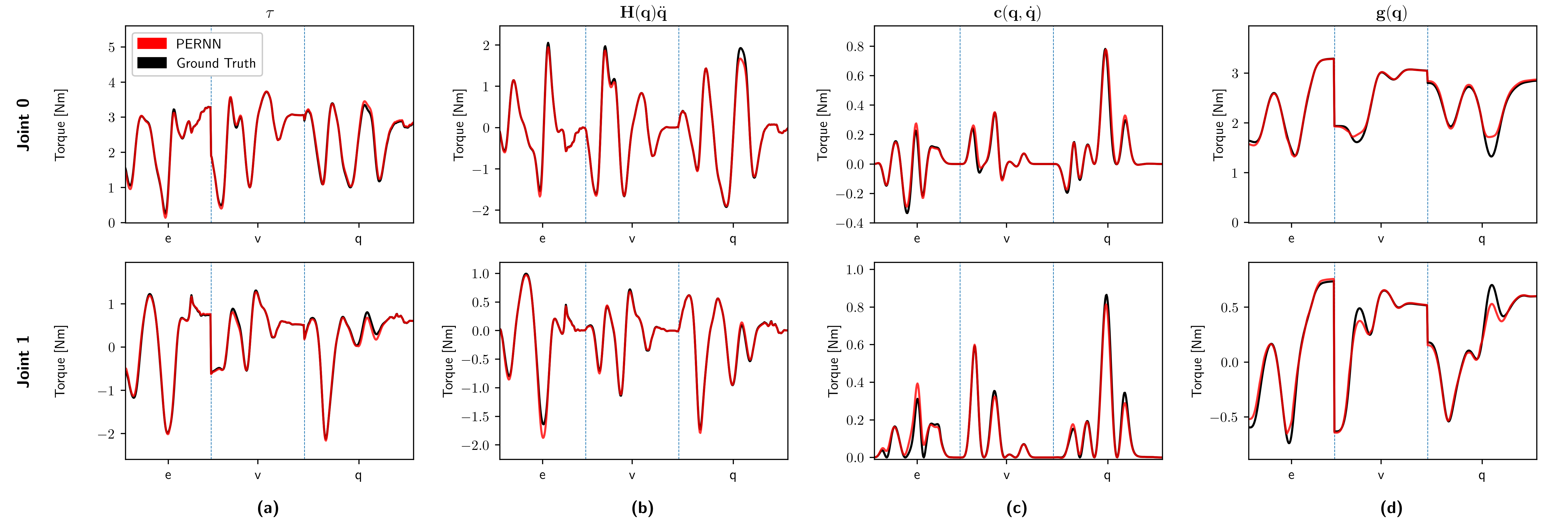
(b) The torque $\tau$ required to generate the characters ’e’, ’v’ and ’q’ in black. Using these samples PERNN was trained offline and learns the red trajectory. Using Equation 1 PERNN can represent the inertial force $\textbf{H}(\ddot{\textbf{q}})$, (b), the Coriolis and Centrifugal forces $\textbf{c}(\textbf{q},\dot{\textbf{q}})$ (c) and the gravitational force $\textbf{g}(\textbf{q})$ (d)

Figure 11: Comparison of DeLaN and PERNN (our method) in terms of closeness to ground-truth. Both models can not only learn the desired torques but also disambiguate the individual torque components even though they were trained on the super-imposed torques. It can be seen that the PERNN model generalizes significantly better than the original DeLaN model and presents better accuracy on all measured variables.

Table 3: Numerical results of the experiments comparing the performance of PERNN against DeLaN on 2-dof robotic motion

Model	Torque (MSE)	Inertia (MSE)	Coriolis & Centrifugal (MSE)	Gravitational (MSE)
DeLaN	0.2073	0.41	0.097	0.0223
PERNN	0.00495	0.00458	0.0011	0.0082

5.2 Autonomous Vehicle Simulation

In this section, we present details on the experimentation and results on the problem of modelling steering dynamics in a simulated autonomous vehicle problem. We compare our Physics Encoded Residual Neural Network (PERNN) approach against two methods. The first is based on traditional fully connected neural networks (FCNN) to serve as a baseline for a purely data-driven method. The second method is based on physics-regularized neural networks which are currently one of the most popular generic physics-informed machine learning methods in literature. This is based on applying soft constraints to the learning process by appropriately penalizing the loss function of neural networks. Assuming an external physics model $P$, input variables x, ground truth target variable $y$ and any feed-forward neural network $f$, the loss function of such a physics-informed network is:

$$L=L_{data}+L_{phy}$$

where $L_{data}$ can be any function measuring the similarity between the predicted variable $f(\textbf{x})$ and the target variable $y$, while $L_{phy}$ can be any function measuring the similarity between the predicted variable $f(\textbf{x})$ and the output from the physics model $P(\textbf{x})$. $L_{phy}$ can also represent the degree to which the neural network output satisfies the constraint on the system, which can be an equation such as a partial differential equation. The loss function can also be represented as a weighted sum of $L_{data}$ and $L_{phy}$, where the weight value can be represented as a hyperparameter or learnable parameter. In the context of the experimentation in this section, we do not employ a weighted sum to calculate the loss term. Since it can be argued that the extra loss term $L_{phy}$ “informs” the neural network of the physical properties, we will refer to this approach as Physics Informed Neural Network (PINN) throughout the experimentation section ahead.

The comparisons between the methods presented herewith are drawn in terms of regression metrics on the test dataset and driving performance inside the simulation on unseen tracks. We also analyse the unknown intermediate variables: lookahead distance and heading difference to reference points chosen by our trained PERNN-based agent in different driving scenarios.

5.2.1 Data Generation

To generate data in TORCS as expert demonstrations for our experimentation, we use the implementation of an advanced heuristic-based agent provided by the simulation based on Ahura: A Heuristic-Based Racer for the Open Racing Car Simulator [47]. The details of this implementation are irrelevant to the approach explained in this paper since, theoretically, this expert system can be any high-fidelity and accurate driving model. We generate state and actuator values at each time instance on each of the 36 race tracks in the simulation, corresponding to two driving scenarios: empty road and traffic bourne. We refer to these two collected datasets as $\mathcal{D}_{1}$ and $\mathcal{D}_{2}$.

The race tracks are divided into three categories: road, dirt and oval speedway tracks based on variations in track geometry. Most of the oval speedway tracks offer relatively simple geometry compared to the more complex geometry on the road tracks in terms of sharpness and variation in the directions of turns. The dirt tracks offer significantly tougher terrain owing to sharper turns and high variation in the altitude values leading to dips and troughs, represented as the $z$ value in Table 1. Figure 12 shows a sample of maps representing geometrical variations in each of the three track categories.

We reserve the data from a set of tracks as our test cases from both $\mathcal{D}_{1}$ and $\mathcal{D}_{2}$, where we analyze the behaviour of the trained models in the simulation. These include all dirt tracks and several road tracks. The goal is to test how well each approach performs in navigating new geometrical scenarios and their consequent capability for error recovery.

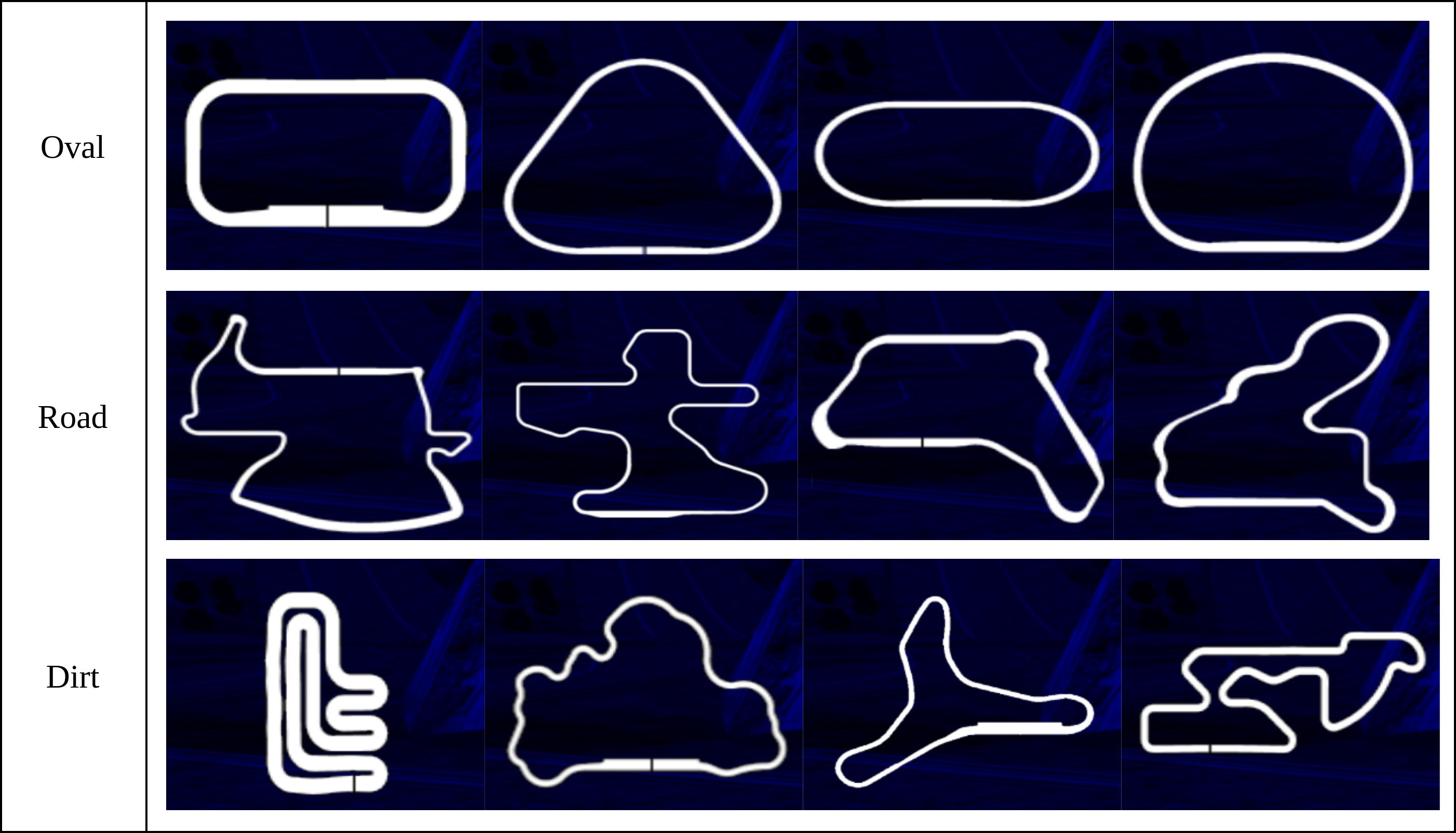
Figure 12: Sample track maps representing geometrical variations in each of the three track categories

5.2.2 Experimental Setup

We test four different agents in our experimentation. The first agent is based on the model trained using our Physics Encoded Residual Neural Network (PERNN) explained earlier in the paper. The second agent is based on the same framework as our method but without the residual block. This will help us illustrate the effectiveness of the residual-based architecture. We will refer to this model as Physics Encoded Neural Network (PENN). The third agent, as a benchmark, is based on a model trained using a conventional feed-forward neural network (FCNN) with a set of fully connected layers and ReLU activation functions. Finally, the fourth type of agent is trained using a physics-informed neural network (PINN) having the same base architecture as the FCNN. The output from all networks is a single steering value based on the state information provided to the model.

For the PINN approach, the Pure Pursuit model serves as the physics model regularizing the loss function (discussed at the beginning of section 5.2). The Pure Pursuit model takes as input appropriate values of lookahead distance ($l$) and target heading difference ($\theta_{target}$), and since there is no concept of learning blocks predicting intermediate variables in the PINN approach, we use our heuristic function from section 4.2.3 to generate these values for each data point in the training data. This means that the regularizing term $L_{phy}$ is calculated for empty road scenarios where the logic behind the heuristic function holds. For the traffic-based data points, $L_{phy}$ is set to zero to not influence the loss value for traffic-based scenarios.

For experimental coherence, we use a simple PID controller to control the speed and brake of the vehicle and a basic functional logic to control the gears based on the vehicle’s speed. The controller’s implementation details are irrelevant to the experiment results since they are kept constant for both driving agents.

We compare three different FCNN models with our PERNN model regarding mean absolute error (MAE) on the test dataset, average distance travelled, and average jerk in predicted steering on the test tracks during live simulation. The three FCNN models are trained on the collective data from $\mathcal{D}_{1}$ and $\mathcal{D}_{2}$, comprising a single phase of training, as opposed to the two-phased setup for the PERNN model (see section 4.2.3). The three FCNN models differ in architectural complexity and training data size (number of tracks comprised in training data) as shown in Table 4. Since the size of the training data and the number of parameters in the model are related in terms of the bias-variance trade-off, each of the three FCNN models consumes a differing, dedicated size of training data for fair comparison.

We also compare the performance of the agents using two key driving metrics. The first metric is a macro-level statistic of the average distance travelled by the agents on the test tracks before they hit the road boundaries. The second, more micro-level metric is based on the smoothness factor of the driving trajectory. This is shown through the jerk and entropy values associated with the predicted steering angle during the test runs. Jerk is a third-order derivative of the predicted steering angle. If we refer to the predicted steering angle as $\delta$, then the steering velocity is calculated as $\delta^{\prime}$, steering acceleration as $\delta^{\prime\prime}$ and finally the jerk value as $\delta^{\prime\prime\prime}$.

To keep experimental consistency, the PENN architecture for the learning and physics blocks is kept the same as that in the PERNN model. In addition, the PINN-based model architecture is kept the same as the smallest FCNN model for a direct and fair comparison of the effectiveness of the method in comparison to our approach.

In summary, we investigate the effectiveness of the PERNN model against the FCNN and PINN counterparts based on the two areas:

1. Data requirements include the number of unique tracks as part of the training data.

2. The complexity of the architecture in terms of the number of parameters in the neural network to capture driving behaviour from the expert demonstrations.

5.2.3 Results

Table 4 presents the results of this analysis. It can be seen that the PERNN consumes much less training data (only 6 out of 36 tracks used in training data) compared to the FCNN models in general and is composed of significantly fewer model parameters. Despite this, the PERNN model converges better than the small and medium FCNN models on the test dataset on MAE (Mean Absolute Error). It is important to note that the PENN model comprising no residual blocks struggles to converge on the test dataset owing to restricted gradient flow. The agent based on this model also fails to generalize the learned driving behaviour in the live simulation with a significantly low average distance travelled on the test tracks.

Figure 13 elaborates on the results. Figure 13(a) compares the MAE scores to the number of parameters for each model in the experimentation. The PERNN model shows comparable MAE scores on the test dataset to the FCNN-large model but with approximately 260 times fewer model parameters. Similarly, Figure 13(b) compares MAE scores to training data requirements for each model in the experimentation. Our PERNN model shows comparable MAE scores on the test dataset to the FCNN-large model while using five times less training data in the form of unique tracks in the generated observation data. Both of these observations are a testament to the effectiveness of the physics blocks in the PERNN architecture in providing prior steering knowledge to the model as an inductive bias. Similarly, Figure 14 compares the average distances travelled without collision during the live simulation on test tracks by each agent. PERNN-based agent achieves higher distances compared to FCNN-small, FCNN-medium models and the PINN model while using less training data and comprising fewer parameters.

Figure 15 shows the comparison of the distance successfully manoeuvred by the agent (before the collision with the road boundary) against the jerk produced by the steering (lower the jerk, smoother the driving trajectory). The analysis is carried out for the driving agent based on each model in the experimentation. The PERNN model outperforms FCNN-small and FCNN-medium models regarding both higher average distance travelled and significantly less jerk in predicted steering. The large version of FCNN exhibits better MAE values on the test set compared to the PERNN model and eventually surpasses it in navigating longer patches of tracks during the live simulation. It however suffers from higher values of steering jerk due to the model attempting to recover from cascading errors, a known issue in these methods under Behavioral Cloning settings. Since the PERNN model inherently encodes the basic error recovery function of following the reference point from any arbitrary state, it offers smaller jerk values and a smoother driving trajectory without explicit variations in training data.

It is important to understand the inherent limitation of the PINN approach which is overcome by our PERNN method, allowing better accuracy. Figure 16 illustrates the difference in the distribution of the ground-truth steering values and the steering values generated from the physics model (Pure Pursuit) for empty road scenarios. This forms decoupled targets for the model to learn, which is depicted in the graph to the right of the distribution showing the validation dataset loss values failing to converge anywhere close to the other methods. Despite this, it outperforms FCNN-small (with equal size of training data and number of model parameters) on live simulation on the test tracks in terms of both average distance travelled and average jerk values. This illustrates the benefit in terms of incorporating prior physics knowledge of driving in the model. PERNN takes a step ahead and provides the capability to learn from both the data and the physics using the concept knowledge blocks, facilitated by residual blocks and therefore does not suffer from the decoupled behaviour in physics and data.

Table 4: Numerical results of the experiments comparing the performance of PERNN against FCNN-based agents

Model	Tracks in Train Set	Neural Configuration	Parameters	Test MAE ($rad$)	Avg. Distance($m$)	Avg. Jerk ($rads^{-3}$)
FCNN-small	6	[64, 32, 16, 8, 4, 1]	6977	0.0287	1157	0.0014
FCNN-medium	14	[256, 128, 64, 32, 16, 8, 4, 1]	60801	0.024	2762	0.008
FCNN-large	25	[1024, 512, 256, 128, 64, 32, 16, 8, 4, 1]	767617	0.01	3803	0.0347
PINN	6	[64, 32, 16, 8, 4, 1]	6977	0.077	1958	0.0001
PERNN	6	Learning Block: [32, 16, 8, 2] + Residual Block: [8, 4, 1] + PhysBlock	5611	0.0214	3209	0.00003
PENN	6	Learning Block: [32, 16, 8, 2] + PhysBlock	2794	0.0364	275	0.0016

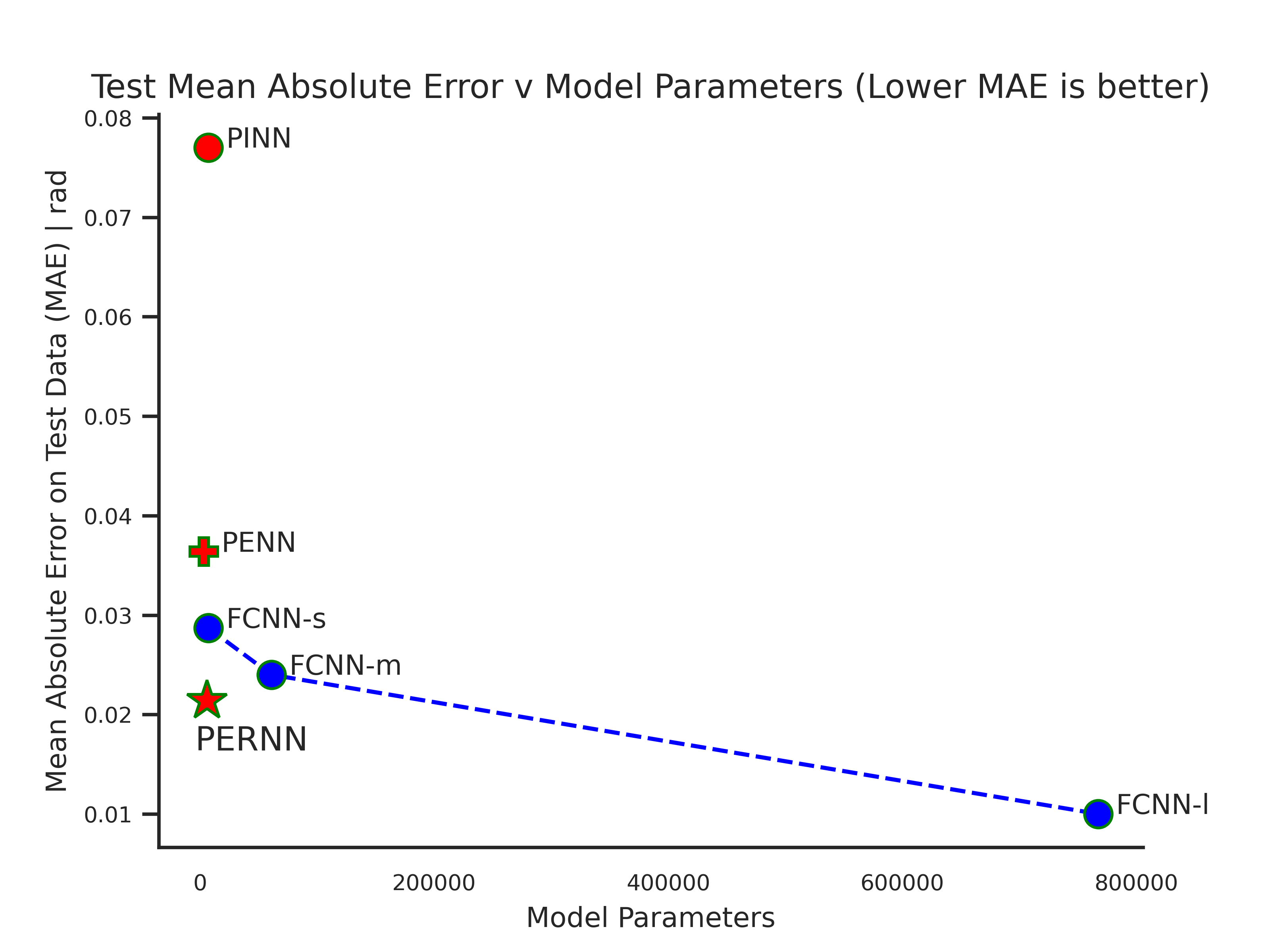
(a) Comparison of MAE score to model parameters for each model in the experimentation. Our PERNN model shows comparable MAE scores on the test dataset to the FCNN-large model but with approximately 260 times fewer model parameters. This is due to the physics blocks providing prior steering knowledge to the model as an inductive bias

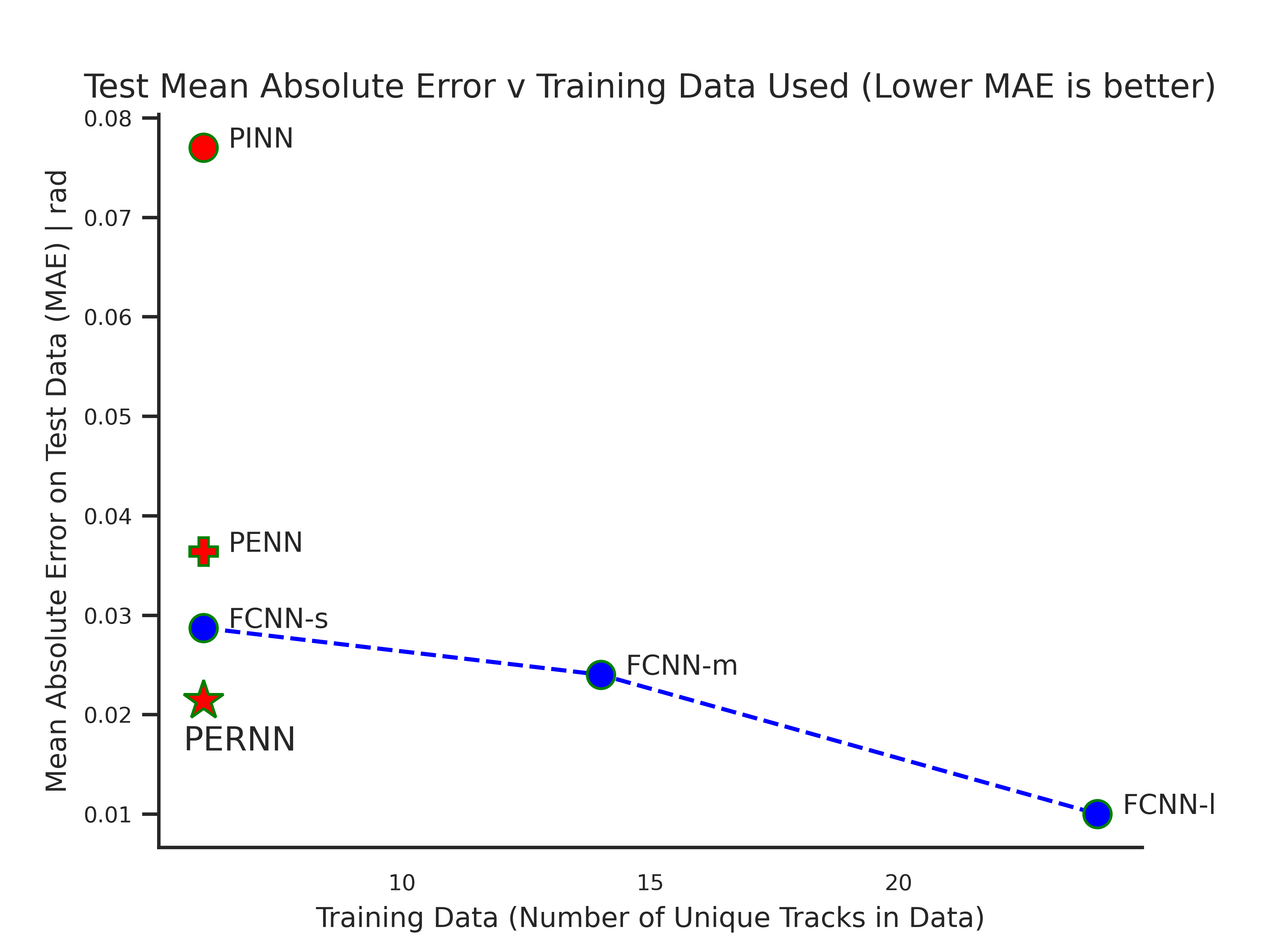
(b) Comparison of MAE score to training data requirements for each model in the experimentation. Our PERNN model shows comparable MAE scores on the test dataset to the FCNN-large model while using five times less training data in the form of unique tracks in the generated observation data. This is due to the physics blocks providing prior steering knowledge to the model as an inductive bias.

Figure 13: Comparison of model accuracy (Mean Absolute Error), number model of parameters and training data requirements.

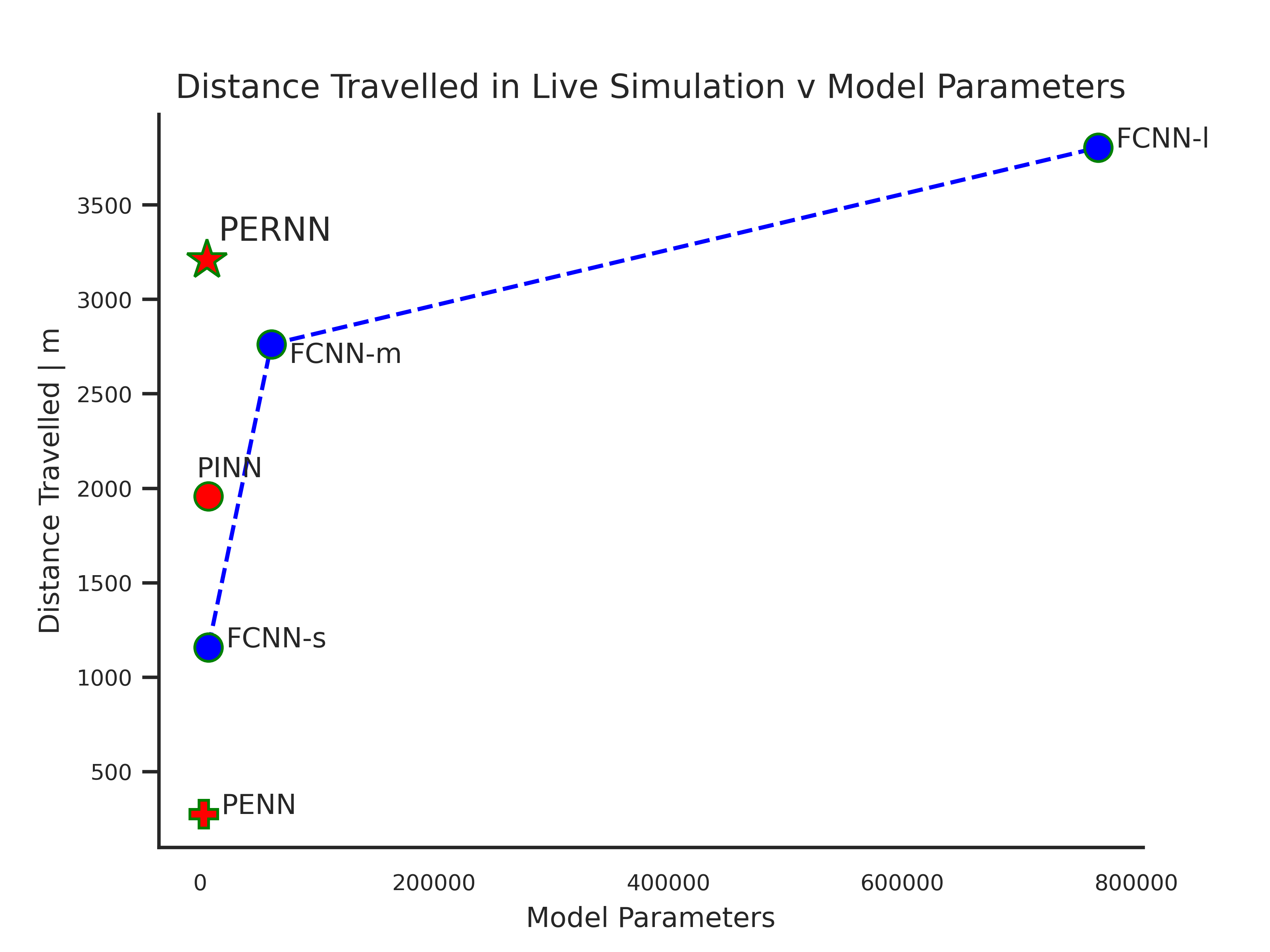
(a) Comparison of distance successfully manoeuvred by the agent (before the collision with road boundary) on test tracks against model parameters for each model in the experimentation. The PERNN model outperforms all other approaches except FCNN-large with lesser model complexity.

(b) Comparison of distance successfully manoeuvred by the agent (before the collision with road boundary) on test tracks against unique tracks used in training data for each model in the experimentation. The PERNN model outperforms all other approaches except FCNN-large with lesser training data.

Figure 14: Comparison of distance travelled by agent in simulation on test tracks, number model of parameters and training data requirements.

Figure 15: Comparison of the distance successfully manoeuvred by the agent (before the collision with road boundary) on test tracks against the jerk produced by the steering (lower the jerk, smoother the driving trajectory). The experiment is carried out for each model. The PERNN model achieves a comparable successful distance travelled to the FCNN-large model but with significantly smaller jerk values, indicating a smoother driving trajectory.

Figure 16: Distribution of target steering values from the observation (ground-truth) data and the physics model in the PINN approach (shown to the left). The decoupled distributions lead to the loss function struggling to converge on the training and validation dataset (shown to the right).

5.2.4 Analysis of Unobserved Intermediate Variables

Another key benefit of the PERNN model is that it predicts the intermediates variables, the lookahead distance and heading difference values which are not explicitly part of the observation data from the driving environment. We analyse the distribution of these variables for a set of road scenarios to analyse the agent’s decision-making based on the PERNN model predictions. This is specifically defined using the range finder sensors $R$ and $O$ (see Table 1), for filtering examples based on the relative distances from the track edge and traffic vehicles on either side of the vehicle in the driving space ahead. Index value $9$ in both $R$ and $O$ suggests distances to objects in the direction of the vehicle’s heading (straight ahead).

We divide the road scenarios in the test data into three simplified categories:

• Category A: Scenarios with relatively more space towards the right of the driving space ahead. The data points in the set follow the principle that for distances defined in vectors $R$ and $O$:

  $$R_{10}>R_{8}+20$$

  $$O_{10}>O_{8}+20$$

  This implies that the track boundary or vehicle at 10 degrees to the left of the agent vehicle is at least 20m further compared to the track boundary or vehicle at 10 degrees to the right of the vehicle’s direction.

• Category B: Scenarios with relatively more space towards the left of the driving space ahead. The data points in the set follow the principle that for distances defined in vectors $R$ and $O$:

  $$R_{8}>R_{10}+20$$

  $$O_{8}>O_{10}+20$$

  This implies that the track boundary or vehicle at 10 degrees to the right of the agent vehicle is at least 20m further compared to the track boundary or vehicle at 10 degrees to the left of the vehicle’s direction.

• Category C, where there is limited space on either side, and a traffic vehicle is situated at the center in front. This makes scenarios where overtaking is improbable. The data points in the set follow the principle that for distances defined in vectors $R$ and $O$:

  $$R_{8}<40\quad\text{and}\quad R_{10}<40$$

  $$O_{8}<40\quad\text{and}\quad O_{10}<40$$

  $$O_{9}<70$$

  This implies that the track boundary or vehicle at 10 degrees to the right and left of the agent vehicle’s direction of motion is less than $40m$ and that there is a vehicle in front at a distance of less than $70m$.

The values for the distance bounds are empirically found to depict the behaviour most vividly and can be set as any arbitrary value based on the concept of the three category divisions. Figure 17 illustrates the results of this analysis. The distribution of the predicted heading angle for the Category A dataset clearly shows a right skew, suggesting that the model mostly selected points that were to the right side of the driving space in the front. Similarly, for Category B, the left skew is vividly depicted, which is understandable based on the specifications of the scenarios. The heading difference in Category C is slightly more evenly distributed despite a right skew. It could be inferred that the reference agent preferred to stay more towards the right in this scenario, which behaviour the PERNN model captured. It can be seen that the lookahead distance distribution is generally less uniform for Category A and B compared to Category C. This is understandable since Category C comprises more restricted scenarios based on available driving space for the agent.

The encouraging results of this analysis suggest the PERNN model offers significantly more explainability compared to conventional neural networks through the discovery of unknown, human-understandable variables in the environment.

Figure 17: An analysis of the model rationale in predicting the intermediate variables in the environment. The plot shows distributions of the intermediate variables, target angle (heading difference) and lookahead distance to the selected point on the road by the PERNN-based agent. Each category is represented as a row of two distribution plots.

6 Conclusion and Future Work

This paper presents a novel physics-encoded neural network architecture for embedding physics models into neural networks. The concept of residual knowledge blocks allows this architecture to be used as a general framework for encoding physics knowledge into neural networks using any differentiable physics model. It is a promising research direction in terms of adding reliability and interpretability to neural network-based learning algorithms by providing the capability to discover unknown variables in the environment which are not part of the originally observed data. Furthermore, this method provides a direct and effective way to build prototype models rapidly for the general digital twin scenarios with limited data and physical definitions of real-world entities.

We investigated our method in two distinct applications. The first involved modelling basic robotic motion using Euler-Lagrangian equations of motion as physics prior. We extended the current state-of-the-art method (DeLaN) to build our residual knowledge blocks and presented the effectiveness of the residual methodology in the context of our general physics-encoded neural network framework. The second application involved developing a steering model for autonomous vehicles in the TORCS simulation environment. We presented some key achievements here, including significantly improved generalizability of the driving model to new road scenarios compared to pure data-driven, fully-connected neural networks and the well-known physics informed (regularized) neural network method. This was achieved with much less model complexity and data requirements. We showed that this method outperformed both counterparts on unseen test track scenarios regarding driving metrics like average distance travelled before boundary hit and smoothness of steering trajectory. We presented an analysis of the effectiveness of our method to discover unknown variables such as the lookahead distance and the heading difference to the selected point on the road and how the model intelligently predicted these variables based on different road scenarios. This also presented valuable insight regarding the explainability of the model’s decision-making based on what point on the road is selected to be followed for different scenarios.

It would be promising to test this approach further on a wide range of problems - specifically in the digital twin space where data availability is constrained and physics models are ‘ab-inito’ or first principle. Further study on the behaviour of gradient flow through the network could help develop more robust residual blocks, especially for more complex physics where large physics blocks could present more constraints on the algorithm’s convergence.

Declarations

• Funding: The research presented in this manuscript is supported by BT (British Telecom) PLC, and two Engineering and Physical Sciences Research Council (EPSRC) grants: AI-driven Digital Twins for Net Zero (EP/Y00597X/1) and Clinical Care (EP/Y018281/1)

• Conflict of interest/Competing interests: The IP for this work is owned by BT PLC, and as part of the agreement, the patent for this work has been filed before submitting the document to the journal.

• Ethics approval: The experiments were performed on data not related to living beings. No human beings and animals were involved in conducting the experiments. Thus, approval from an ethical committee is not required.

• Consent to participate: No living beings are involved in conducting the experiments for this research. Thus, consent to participate is not required.

• Consent for publication: The authors involved in conducting this research give their consent for the publication of the article titled “Physics Encoded Blocks in Residual Neural Network Architectures for Digital Twin Models”.

• Availability of data and materials: The simulation and agents used to generate data and test agents in this research are available online. The references and citations are provided in this manuscript.

• Code availability: The code has been made available on GitHub. https://github.com/saadzia10/Physics-Encoded-ResNet.git

• Authors’ contributions: Muhammad Saad Zia and Ashiq Anjum have equal contributions to this manuscript. Lu Liu is an academic reviewer and collaborator on the work in this manuscript. Anthony Conway and Anasol Peña-Rios are industrial collaborators on the work in this manuscript.

References

- [1] K. E. Willcox, O. Ghattas, and P. Heimbach, ”The imperative of physics-based modeling and inverse theory in computational science,” Nat Comput Sci, vol. 1, pp. 166-168, 2021. https://doi.org/10.1038/s43588-021-00040-z
- [2] J. Wang, Y. Li, R. Gao, and F. Zhang, ”Hybrid physics-based and data-driven models for smart manufacturing: Modelling, simulation, and explainability,” Journal of Manufacturing Systems, vol. 63, pp. 381-391, 2022. https://doi.org/10.1016/j.jmsy.2022
- [3] A. Rasheed, O. San, and T. Kvamsdal, ”Digital Twin: Values, Challenges and Enablers From a Modeling Perspective,” IEEE Access, vol. 8, pp. 21980-22012, 2020. https://doi.org/10.1109/ACCESS.2020.2970143
- [4] A. Thelen, X. Zhang, O. Fink, et al., ”A comprehensive review of digital twin — part 1: modeling and twinning enabling technologies,” Struct Multidisc Optim, vol. 65, p. 354, 2022. https://doi.org/10.1007/s00158-022-03425-4
- [5] L. Lu, P. Jin, G. Pang, Z. Zhang, and G. E. Karniadakis, ”Learning nonlinear operators via DeepONet based on the universal approximation theorem of operators,” Nat. Mach. Intell., vol. 3, pp. 218-229, 2021.
- [6] Darbon, J. and Meng, T. ”On some neural network architectures that can represent viscosity solutions of certain high dimensional Hamilton-Jacobi partial differential equations,” J. Comput. Phys. 425, 109907, 2021
- [7] Y. Li, J. Wu, J.-Y. Zhu, J. B. Tenenbaum, A. Torralba, and R. Tedrake, ”Propagation networks for model-based control under partial observation,” in IEEE International Conference on Robotics and Automation (ICRA), 2019.
- [8] M. Toussaint, K. R. Allen, K. A. Smith, and J. B. Tenenbaum, ”Differentiable physics and stable modes for tool-use and manipulation planning,” in IEEE International Conference on Robotics and Automation (ICRA), 2018.
- [9] A. Sanchez-Gonzalez, N. Heess, J. T. Springenberg, J. Merel, M. Riedmiller, R. Hadsell, and P. Battaglia, ”Graph networks as learnable physics engines for inference and control,” in International Conference on Machine Learning (ICML), 2018.
- [10] K. He, X. Zhang, S. Ren and J. Sun, ”Deep Residual Learning for Image Recognition,” 2016 IEEE Conference on Computer Vision and Pattern Recognition (CVPR), Las Vegas, NV, USA, 2016, pp. 770-778, doi: 10.1109/CVPR.2016.90.
- [11] J. Seo, B. D. Smith, S. Greydanus, S. Saha, C. Paduraru, C. Wan, A. Bansal, G. Jain, A. Peng, S. Narvekar, G. Pezeshki, E. Brevdo, C. X. Moore, S. Patel, H. Wang, J. Merel, K. Tunyasuvunakool, N. Heess, R. Hadsell, and S. Varma, ”Learning to optimize complex real-world systems through automated differentiation & differentiable programming,” in Conference on Neural Information Processing Systems (NeurIPS), 2022.
- [12] R. Stewart and S. Ermon, ”How to train your differentiable physical simulator,” in NeurIPS Workshop on Machine Learning for Physics and the Physical Sciences (ML4PS), 2019.
- [13] S. Greydanus, M. Dzamba, and J. Yosinski, ”Hamiltonian neural networks,” in Conference on Neural Information Processing Systems (NeurIPS), 2019.
- [14] M. Raissi, P. Perdikaris, and G. E. Karniadakis, ”Physics-informed neural networks: A deep learning framework for solving forward and inverse problems involving nonlinear partial differential equations,” Journal of Computational Physics, vol. 378, pp. 686-707, 2019.
- [15] M. Cranmer, S. Greydanus, S. Hoyer, P. Battaglia, D. Spergel, and S. Ho, ”Lagrangian neural networks,” in International Conference on Learning Representations (ICLR), 2020.
- [16] D. Mrowca, C. Zhuang, E. Wang, N. Haber, L. F. Fei-Fei, J. Tenenbaum, and D. Yamins, ”Flexible neural representation for physics prediction,” in Conference on Neural Information Processing Systems (NeurIPS), 2018.
- [17] A. Ajay, J. Wu, N. Fazeli, M. Bauza, L. P. Kaelbling, J. B. Tenenbaum, and A. Rodriguez, ”Augmenting physical simulators with stochastic neural networks: Case study of planar pushing and bouncing,” in IEEE/RSJ International Conference on Intelligent Robots and Systems (IROS), 2018.
- [18] A. Mohan, H. Chai, M. J. Khojasteh, D. Dey, and K. Joshi, ”CDPN: Coordinated differentiable physics networks for interacting rigid bodies,” in Conference on Neural Information Processing Systems (NeurIPS), 2021.
- [19] M. Lutter, C. Ritter, and J. Peters, ”Deep Lagrangian Networks: Using Physics as Model Prior for Deep Learning” in International Conference on Learning Representations, 2019. [Online]. Available: https://openreview.net/forum?id=BklHpjCqKm.
- [20] A. Kashefi, D. Rempe, and L. J. Guibas, ”A point-cloud deep learning framework for prediction of fluid flow fields on irregular geometries,” Phys. Fluids, vol. 33, p. 027104, 2021.
- [21] Z. Li et al., ”Fourier neural operator for parametric partial differential equations,” in Int. Conf. Learn. Represent., 2021.
- [22] M. Raissi, P. Perdikaris, and G. E. Karniadakis, ”Physics-informed neural networks: a deep learning framework for solving forward and inverse problems involving nonlinear partial differential equations.”
- [23] I. E. Lagaris, A. Likas, and D. I. Fotiadis, ”Artificial neural networks for solving ordinary and partial differential equations,” IEEE Trans. Neural Netw., vol. 9, pp. 987-1000, 1998.
- [24] Y. Zhu, N. Zabaras, P. S. Koutsourelakis, and P. Perdikaris, ”Physics-constrained deep learning for high-dimensional surrogate modeling and uncertainty quantification without labeled data,” J. Comput. Phys., vol. 394, pp. 56-81, 2019.
- [25] N. Geneva and N. Zabaras, ”Modeling the dynamics of PDE systems with physics-constrained deep auto-regressive networks,” J. Comput. Phys., vol. 403, p. 109056, 2020.
- [26] J. L. Wu et al., ”Enforcing statistical constraints in generative adversarial networks for modeling chaotic dynamical systems,” J. Comput. Phys., vol. 406, p. 109209, 2020.
- [27] I. E. Lagaris, A. Likas, and D. I. Fotiadis, ”Artificial neural networks for solving ordinary and partial differential equations,” IEEE Trans. Neural Netw., vol. 9, pp. 987-1000, 1998.
- [28] R. S. Beidokhti and A. Malek, ”Solving initial-boundary value problems for systems of partial differential equations using neural networks and optimization techniques,” J. Franklin Inst., vol. 346, pp. 898-913, 2009.
- [29] B. Wang, W. Zhang, and W. Cai, ”Multi-scale deep neural network (MscaleDNN) methods for oscillatory stokes flows in complex domains,” Commun. Comput. Phys., vol. 28, pp. 2139-2157, 2020.
- [30] W. Cai, X. Li, and L. Liu, ”A phase shift deep neural network for high frequency approximation and wave problems,” SIAM J. Sci. Comput., vol. 42, pp. A3285-A3312, 2020.
- [31] J. Darbon and T. Meng, ”On some neural network architectures that can represent viscosity solutions of certain high dimensional Hamilton-Jacobi partial differential equations,” J. Comput. Phys., vol. 425, p. 109907, 2021.
- [32] C. Miles, G. Sam, H. Stephan, B. Peter, S. David, and H. Shirley, ”Lagrangian neural networks,” in International Conference on Learning Representations, Workshop on Integration of Deep Neural Models and Differential Equations, 2020.
- [33] J. Degrave, M. Hermans, J. Dambre, and F. Wyffels, ”A differentiable physics engine for deep learning in robotics,” Frontiers in Neurorobotics, vol. 13, article 6, 2019.
- [34] P. Holl, V. Koltun, and N. Thuerey, ”Learning to control PDEs with differentiable physics,” arXiv preprint arXiv:2001.07457, 2020.
- [35] S. Zhu, R. Clement, J. McCalmon, C. Davies and T. Hill, ”Stable gap-filling for longer eddy covariance data gaps: A globally validated machine-learning approach for carbon dioxide, water, and energy fluxes”, Agricultural and Forest Meteorology, vol. 314, p. 108777, 2022.
- [36] G. Lasslop, M. Reichstein, D. Papale, A. Richardson, A. Arneth, A. Barr, P. Stoy, and G. Wohlfahrt, ”Separation of net ecosystem exchange into assimilation and respiration using a light response curve approach: critical issues and global evaluation,” Global Change Biology, vol. 16, no. 1, pp. 187-208, 2010. https://doi.org/10.1111/j.1365-2486.2009.02041.x
- [37] T. F. Keenan, M. Migliavacca, D. Papale, et al., ”Widespread inhibition of daytime ecosystem respiration,” Nature Ecology and Evolution, vol. 3, pp. 407-415, 2019. https://doi.org/10.1038/s41559-019-0809-2
- [38] J. Lloyd and J. A. Taylor, ”On the temperature dependence of soil respiration,” Functional Ecology, vol. 8, no. 3, pp. 315-323, 1994. http://www.jstor.org/stable/2389824
- [39] M. Reichstein, E. Falge, D. Baldocchi, et al., ”On the separation of net ecosystem exchange into assimilation and ecosystem respiration: review and improved algorithm,” Global Change Biology, vol. 11, pp. 1424-1439, 2005.
- [40] E. Espié, C. Guionneau, B. Wymann, C. Dimitrakakis, R. Coulom, and A. Sumner, ”TORCS, The Open Racing Car Simulator,” 2005.
- [41] J. Degrave, M. Hermans, J. Dambre, and F. Wyffels, ”A differentiable physics engine for deep learning in robotics,” Frontiers in Neurorobotics, vol. 13, p. 42, 2019.
- [42] P. Christiano, J. Leike, T. Brown, M. Martic, S. Legg, and D. Amodei, ”Deep reinforcement learning from human preferences,” 2017.
- [43] P. Abbeel and A. Y. Ng, ”Apprenticeship learning via inverse reinforcement learning,” in Proceedings of the twenty-first international conference on Machine learning (ICML ’04), New York, NY, USA, 2004, pp. 1. https://doi.org/10.1145/1015330.1015430
- [44] J. Broekens and M. Bruijnes, ”Learning from human-generated reinforcement for simulated characters,” in Proceedings of the 10th International Conference on Intelligent Virtual Agents, Springer, 2010, pp. 179-185.
- [45] O. Cappé, I. Chades, and Y. Guan, ”Calibration of stochastic simulation models,” in The Oxford Handbook of Bayesian Econometrics (Vol. 3), Oxford University Press, 2017, pp. 105-135.
- [46] S. Ali, S. A. A. Shah, M. S. Nawaz, and M. Shah, ”Survey on crowd simulation: Techniques and methodologies,” Applied Sciences, vol. 9, no. 14, p. 2941, 2019.
- [47] M. R. Bonyadi, Z. Michalewicz, S. Nallaperuma, and F. Neumann, ”Ahura: A Heuristic-Based Racer for the Open Racing Car Simulator,” IEEE Transactions on Computational Intelligence and AI in Games, vol. 9, no. 1, pp. 54-66, 2017. DOI: 10.1109/TCIAIG.2016.2565661.