A Map of the Orbital Landscape for Perturbing Planet Solutions
for Single-Planet Systems with TTVs

Abstract

There are now thousands of single-planet systems observed to exhibit transit timing variations (TTVs), yet we largely lack any interpretation of the implied masses responsible for these perturbations. Even when assuming these TTVs are driven by perturbing planets, the solution space is notoriously multi-modal with respect to the perturber’s orbital period and there exists no standardized procedure to pinpoint these modes, besides from blind brute force numerical efforts. Using $N$-body simulations with TTVFast and focusing on the dominant periodic signal in the TTVs, we chart out the landscape of these modes and provide analytic predictions for their locations and widths, providing the community with a map for the first time. We then introduce an approach for modeling single-planet TTVs in the low-eccentricity regime, by splitting the orbital period space into a number of uniform prior bins over which there aren’t these degeneracies. We show how one can define appropriate orbital period priors for the perturbing planet in order to sufficiently sample the complete parameter space. We demonstrate, analytically, how one can explain the numerical simulations using first-order near mean-motion resonance super-periods, the synodic period, and their aliases – the expected dominant TTV periods in the low-eccentricity regime. Using a Bayesian framework, we then present a method for determining the optimal solution between TTVs induced by a perturbing planet and TTVs induced by a moon.

1 Introduction

Exoplanet transits occur when a planet passes in front of its host star, blocking a portion of the light. If the timing of the transit isn’t perfectly periodic, the planet is said to exhibit transit timing variations (TTVs). If physical, these TTVs are caused by gravitational interactions with other masses, typically assumed to be companion planets (e.g., Dobrovolskis & Borucki, 1996; Miralda-Escudé, 2002; Holman & Murray, 2005; Agol et al., 2005; Lithwick et al., 2012; Nesvorný & Vokrouhlický, 2014; Schmitt et al., 2014; Deck & Agol, 2015; Agol & Fabrycky, 2018). In this case, TTVs are the results of minor variations (or wobbles) in the planet’s orbit. Stellar activity is the biggest cause of spurious TTV signals, as star spots and other stellar activity signals on rotating stars can mimic a TTV of a physical nature (e.g., Sanchis-Ojeda et al., 2011; Mazeh et al., 2013; Szabó et al., 2013; Oshagh et al., 2013; Holczer et al., 2015; Mazeh et al., 2015; Ioannidis et al., 2016; Siegel & Rogers, 2022).

Planet-planet TTVs have long been recognized as a valuable observational resource for precise characterization of planets down to even Earth masses (Agol et al., 2005; Holman & Murray, 2005) and have been used for some of the most precise characterization of planetary parameters in multi-planet systems (e.g., TRAPPIST-1 with precision equivalent to radial velocity precision of 2.5 cm s${}^{-}1$ in Agol et al., 2021). For a thorough introduction to planet-planet TTVs we point the reader to Agol & Fabrycky (2018) – but a brief overview follows.

In short, the amplitude of TTVs is proportional to a planets’ own orbital period as planets gravitationally interact on the the orbital timescale. As the acceleration of a body doesn’t depend on its own mass, TTVs of each planet scale with the mass of the other bodies in the system and are insensitive to their own mass. In a two planet system, if we define $P_{0}$ and $P_{1}$ as the orbital periods of the two planets, $m_{0}$, $m_{1}$, and $m_{2}$ as the masses of the star and two planets, respectively, and $f_{ij}$ (a function of semi- major axis ratio, $\alpha_{ij}=\mathrm{min}(a_{i}/a_{j},\,a_{j}/a_{i})$) describes the perturbations of planet $j$ on planet $i$ and the angular orbital elements of the planets $\theta_{ij}=(\lambda_{i},e_{i},\omega_{i},I_{i},\Omega_{i},\lambda_{j},e_{j},\omega_{j},I_{j},\Omega_{j})$, then to lowest order in mass ratio, the $O-C$ TTVs ($\delta t_{1}$ and $\delta t_{2}$) can be expressed as

$$\delta t_{1}=P_{1}\frac{m_{2}}{m_{0}}f_{12}(\alpha_{12},\,\theta_{12}),$$ (1)

$$\delta t_{2}=P_{2}\frac{m_{1}}{m_{0}}f_{21}(\alpha_{21},\,\theta_{21}).$$ (2)

For more on how to evaluate these functions, see Nesvorný & Morbidelli (2008); Nesvorný (2009); Nesvorný & Beaugé (2010); Agol & Deck (2016); Deck & Agol (2016). If there are more than two planets in the system, the mass-ratios of the planets to the star are sufficiently small, and none of the planet-pairs are in a mean-motion resonance (MMR), then the TTVs are well approximated as a linear combination of the perturbations due to each companion planet. In this case, for $N$ planets, the TTVs for planets $i=1,2,...,N$ can be expressed as

$$\delta t_{i}=P_{i}\sum_{j\neq i}\frac{m_{j}}{m_{0}}f_{ij}(\alpha_{ij},\,\theta_{ij}).$$ (3)

The largest planet-planet TTVs are induced by orbital period changes that occur due to librations of the system about a MMR. The amplitudes of these TTVs can be calculated via conservation of energy (Agol et al., 2005; Holman et al., 2010). Close to resonances, changes to both the semi-major axes and eccentricities lead to TTV cycles with a period that depends on the distance from resonance (Steffen, 2006; Lithwick et al., 2012), often called the “super-period” of near-MMR planets. The dominant TTV variation is caused by the system to which its resonance is closest to, for which the critical angles are allowed to move slowly and thus effect the build up. If a planet with period ratio $P_{2}/P_{1}$ is within a few percent of the ratio $j/k$ (integers), then the expected TTV super-periood is

$$P_{\mathrm{TTV}}=P_{\mathrm{sup}}=\frac{1}{|j/P_{1}-k/P_{2}|}.$$ (4)

The strength of the resonance scales with the planet eccentricities to a power the order, where the order of the resonance is defined as $|j-k|$ (i.e., for first-order resonances, there is a linear dependence on eccentricity). Thus, in the low-eccentricity regime, first-order eccentricities are expected to dominate. Eccentricities in multi-planet systems have been largely found to be small in Kepler data, both via the photoeccentric effect (Van Eylen & Albrecht, 2015) and via TTVs (Hadden & Lithwick, 2014). Thus, first-order super-periods are likely the driving force of much of the detectable planet-planet TTVs.

Additional, non-resonant, perturbations occur on the timescale of planetary conjunctions, which is when the planets separation is smallest and thus gravitational attraction is strongest. Conjunctions occur with a period equal to the synodic period,

$$P_{\mathrm{TTV}}=P_{syn}=\frac{1}{|1/P_{\mathrm{1}}-1/P_{\mathrm{2}}|}.$$ (5)

Conjunction-induced TTVs (a.k.a. synodic or “chopping” TTVs) have smaller amplitudes than near-MMR TTVs as they do not add coherently and commonly show TTVs that alternate early and late on top of the larger amplitude near-MMR TTVs. Conjunction-induced TTVs have been demonstrated to be a useful tool in breaking the mass-eccentricity degeneracy inherent in near-MMR TTVs (Nesvorný & Vokrouhlický, 2014; Schmitt et al., 2014; Deck & Agol, 2015).

Aliases are frequent in TTV observations due to the limited sampling rate of transit data. Transits can only be observed with a minimum period equal to its orbital period. Thus, the Nyquist period for TTVs, which defines the minimum recoverable period for a dataset, is equal to twice the orbital period of the transiting planet (Nyquist, 1928; Shannon, 1949). Any TTV with a faster period that the Nyquist period won’t be observed with its true TTV period, but rather at an aliased period, greater than its true period and the Nyquist period limit. In order to determine the observable aliased period, we follow the same derivation as presented in McClellan et al. (1998), and then adopted in Dawson & Fabrycky (2010) for radial velocities and subsequently in Kipping (2021) for TTVs. We find that the observed aliased TTV frequency peaks, $\nu$, in terms of the non-aliased physical TTV period, $P_{\mathrm{TTV}}$, and the period of the transiting exoplanet, $P_{\mathrm{trans}}$, occur at

$$\nu=|\frac{1}{P_{\mathrm{TTV}}}+m\frac{1}{P_{\mathrm{trans}}}|,$$ (6)

where $m$ is a non-zero real integer. Or, in terms of observable aliased TTV periods, $\bar{P}_{\mathrm{TTV}}$, we have

$$\bar{P}_{\mathrm{TTV}}=\frac{1}{\nu}=\frac{1}{|\frac{1}{P_{\mathrm{TTV}}}+m\frac{1}{P_{\mathrm{trans}}}|}$$ (7)

Observing both planets transit is beneficial in characterizing a near-resonant TTV signal, as the phases of the planets’ transits and the TTV signals can be compared and thus ambiguity about the period of the perturbing planet is removed (Lithwick et al., 2012). When only a single planet transits, the measured TTVs could result from a perturbing planet being close to a number of different resonances with the transiting planet (Meschiari & Laughlin, 2010). Nesvorný et al. (2012) were the first to successfully discover and completely classify a non-transiting planet via TTVs (and transit duration variations: TDVs) in the Kepler-46 (a.k.a. KOI-872) system. In order to do so, they Fourier-decomposed the TTVs of the transiting planet into at least four significant sinusoids, which all could be identified as the interaction with the non-transiting planet via a different resonance. Finally, TDVs were used to break a degeneracy between two possible near-resonant solutions.

As discussed in Kipping & Yahalomi (2022) and Yahalomi et al. (2024b), TTVs are frequently observed in single transiting planetary systems, where multiple solutions are possible for the unseen perturbing planets’ period via resonant interactions. In this situation, the parameter space is highly degenerate and multi-model with respect to the unseen planet’s orbital period. While nested sampling methods are quite powerful at sampling multi-model parameter spaces, we’ve found that they are unable to effectively sample different resonant commensurable periods, when given a wide uninformative prior on the perturbing planets’ orbital period. This problem becomes additionally difficult when expanding the realm of possible solutions beyond planet-planet TTVs – as TTVs can be additionally induced by moons (e.g., Sartoretti & Schneider, 1999; Simon et al., 2007; Kipping et al., 2009; Kipping, 2009a, b; Awiphan & Kerins, 2013; Heller, 2014; Heller et al., 2016; Kipping & Teachey, 2020). In order to perform model comparison between planet-planet TTVs and planet-moon TTVs, given an observed TTV signal in a single transiting planet system, it is essential to first sufficiently sample the complete parameter space of both possible solutions.

Here, we aim to classify the orbital landscape of planet-planet TTVs by mapping the solution space for TTV period vs. orbital period ratios. This allows us to identify the multi-modalities, which would allow modeler to adopt appropriate priors in order to effectively sample the complete parameter space. One could then run multiple samplers, with priors set around the different commensurable near-resonant periods and then compare the resulting a-posteriori solutions in order to classify the orbital characteristics of an unseen planetary companion.

In what follows, in Section 2, we present numerical $N$-body simulations to investigate the TTV period vs. orbital period space. In Section 3 we discuss the analytic solutions expected due to near MMR and synodic TTVs in the low-eccentricity regime. In Section 4, we compare our numerical and analytic results and discuss the dynamical interpretation of the numerical simulations. Finally, in Section 5 we present a model comparison approach to differentiating between planet induced TTVs and moon induced TTVs.

2 Numerical Simulations

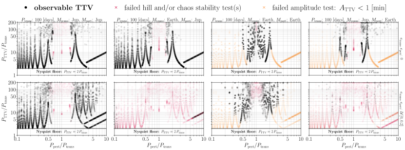
Figure 1: Peak TTV periods recovered via Lomb-Scargle (LS) periodograms fit to transit times simulated with TTVFast. Each column shows a different set of planetary masses. Each row shows a different range of eccentricities. TTVs split into three groups: (i) systems that fail the hill and/or chaos stability criteria (red x markers), (ii) systems with unreliable TTV amplitudes less than 1 minute (orange x markers), (iii) and those that pass both tests and are thus observable TTVs (blue circle markers).

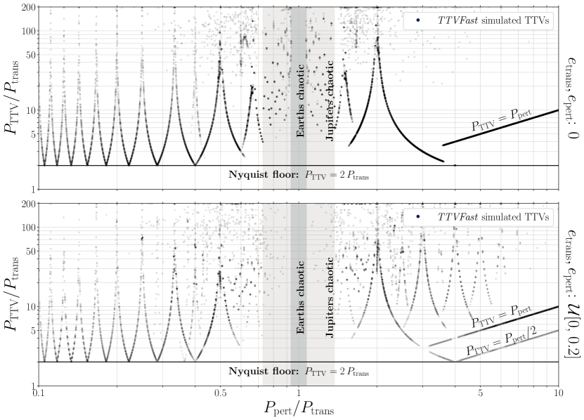
Figure 2: Peak TTV periods recovered via Lomb-Scargle (LS) periodograms fit to TTVFast simulated systems that pass stability and amplitude tests for all combined masses simulated in Figure 1. [Top:] TTVFast systems initialized with zero eccentricity [Bottom:] TTVFast systems initialized with eccentricities between 0 and 0.2. We also show the chaotic boundaries as defined by Deck et al. (2013) for two Earth mass and two Jupiter mass planets, respectively, around a Solar mass star.

We begin by investigating the TTV period vs. orbital period ratio space via numerical ($N$-body) simulations to understand the characteristic periods expected for planet induced TTVs. Our first step was to simulate a large number of two-planet systems and map out the period space ($P_{TTV}$, $P_{trans}$, and $P_{pert}$) of the output TTVs using TTVFast (Deck et al., 2014). TTVFast returns a set of transit times for the simulated planets. We then fit a Lomb-Scargle periodogram (Lomb, 1976; Scargle, 1982) to these transit times, sampling the periodogram in TTV period space, in order to determine for which sets of orbital parameters would TTVs be observable and the dominant periodic TTV signal in these cases. We describe in detail this process, our simulation assumptions and code, and sampling decisions in what follows.

2.1 TTVFast

TTVFast is a dynamical N-body simulation package (Deck et al., 2014) that given a set of input planet parameters computes a set of predicted transit times. TTVFast uses a symplectic integrator with a Keplerian interpolator for the calculation of transit times (Nesvorný et al., 2013). TTVFast optimizes for computational speed, based on the goal of achieving $\sim$1-10 second precision of transit times. This precision is sufficient for our modeling purposes, as it is less than the typical measurement uncertainty of transit timing surveys (Deck et al., 2014).

As we are interested in the low-eccentricity regime, we simulate two different populations of two-planet systems: (i) zero initial eccentricities for both planets and (ii) small initial eccentricities (e $<$ 0.2). We have done so to take a pragmatic approach, as allowing larger eccentricities increases the dependency on higher order super-periods and thus significantly complicates the multi-modality (Murray & Dermott, 1999) and as previously explained, demographically, astronomers have found the eccentricities of planets in multi-planet systems are predominantly small. We note that the eccentricity value here is, as is assumed in TTVFast, an instantaneous eccentricity that is a combination of the free and the forced eccentricity values (Deck et al., 2014).

In our simulations, we simulate coplanar orbits. We adopt this assumption as small mutual inclinations tend to have negligible effects on TTVs (Nesvorný & Vokrouhlický, 2014; Agol & Deck, 2016; Hadden & Lithwick, 2016) and known multi-planet systems appear to be mostly coplanar with typical mutual inclinations less than several degrees (Figueira et al., 2012; Tremaine & Dong, 2012; Fabrycky et al., 2014). For all simulations we simulated a Solar-mass star – but note that the TTV period is scale free with respect to the stellar mass.

We simulated the perturbing planet with a log₁₀-linear grid with 1,000 orbital period values ranging from 1/10 the orbital period of the transiting planet to 100 times the orbital period of the transiting planet. We chose a random initial argument of periastron and mean anomaly for both planets (i.e., random values from the uniform distribution $\mathcal{U}$[0, 360] [deg]). For every simulation, we assume a longitude of ascending node equal to 0 and an inclination equal to 90 [deg].

We fix the orbital period of the transiting planet to 100 days and sample planetary mass pairs of [$M_{\mathrm{trans}}$, $M_{\mathrm{pert}}$] equal to: (i) [Jupiter, Jupiter], (ii) [Earth, Jupiter], (iii) [Earth, Earth], and (iv) [Jupiter, Earth]. Modifying the period of the transiting planet will have an impact on the amplitude of the TTV signal, as previously discussed, but it will not impact the TTV period.

We ran these simulations with TTVFast for a duration equal to 100 times the initial orbital period of the transiting planet with a timestep (dt) equal to 1/20^th the orbital period of the inner planet as suggested in Deck et al. (2014) as larger time steps can lead to step-size chaos and inaccurate orbits (Wisdom & Holman, 1992). We selected 10 different orbital parameter configurations (i.e., sets of eccentricities in each of the relevant ranges, arguments of periastron, and mean anomalies from the distributions described above). For each of the 6 eccentricity ranges, we ran 10,000 TTVFast simulations (1,000 period ratios and 10 sets of random orbital parameters) or 60,000 TTVFast simulations total.

We only keep TTVFast simulations where at least 50 epochs of the transiting planet are returned. This is a conservative cut, as systems in which the inner planet would not have transited at least 50 times during the simulation time scale (100 transit epochs) suggests an orbital period that changed by a factor of greater than two. It is very unlikely, given the long timescale of planetary evolution, that one would observe a stable planet undergoing such rapid dynamical change – and thus we don’t want it to bias our results.

2.2 Lomb-Scargle Periodogram

Following VanderPlas (2018), we fit a Lomb-Scargle (LS) periodogram (Lomb, 1976; Scargle, 1982) to the transit times output from TTVFast. Specifically, we use numpy.linalg.solve to solve the TTV model equation $F(x,\tau,P,\alpha_{\mathrm{TTV}},\beta_{\mathrm{TTV}},P_{\mathrm{TTV}})$. If $x$ is the epoch number, $\tau$ is the time of transit minimum, P is the linear ephemeris transit period, $\alpha_{\mathrm{TTV}}$ & $\beta_{\mathrm{TTV}}$ are the amplitude factors (such that the amplitude of the TTV signal is equal to $\alpha_{\mathrm{TTV}}$ & $\beta_{\mathrm{TTV}}$ added in quadrature), and $P_{\mathrm{TTV}}$ is the dimensionless period of the TTV signal (units of transit epochs), then the linear equation $F(x,\tau,P,\alpha_{\mathrm{TTV}},\beta_{\mathrm{TTV}},P_{\mathrm{TTV}})$ used in our LS periodogram is

$$F(x,\tau,P,\alpha_{\mathrm{TTV}},\beta_{\mathrm{TTV}},P_{\mathrm{TTV}})=$$

$$\tau+P\,x+\alpha_{\mathrm{TTV}}\sin\Bigg{(}\frac{2\pi x}{P_{\mathrm{TTV}}}\Bigg{)}+\beta_{\mathrm{TTV}}\cos\Bigg{(}\frac{2\pi x}{P_{\mathrm{TTV}}}\Bigg{)}.$$

Here, $F(x,\tau,P,\alpha_{\mathrm{TTV}},\beta_{\mathrm{TTV}},P_{\mathrm{TTV}})$ becomes a linear equation once we define $P_{\mathrm{TTV}}$ over a grid with a range between 2 orbits of the transiting planet to twice the number of periods simulated. We setup a TTV period grid evenly spaced in TTV frequency space with a size equal to 10 times the number of transit epochs simulated.

We also use numpy.linalg.solve to solve the null model, $F(x,\tau,P)$ assuming a linear ephemeris (i.e., no TTVs) for the transit times. Here $F(x,\tau,P)$ is

$$F(x,\tau,P)=\tau+P\,x.$$ (9)

For each frequency value in the frequency grid, we determine the $\Delta\chi^{2}$ value by taking the difference between the $\chi^{2}$ values of the TTV model and the linear ephemeris model. Here, we just assume some fiducial homoscedastic error on the times to evaluate the $\chi^{2}$ values. As we are always comparing the $\chi^{2}$ values in determining $\Delta\chi^{2}$, this assumed uncertainty won’t impact the peak solution determination. We then pick the highest $\chi^{2}$ value in the grid and label this the peak TTV solution. As there are multiple periodic components in TTV data, this doesn’t necessarily identify the TTV signal with the peak amplitude. The LS periodogram might pick up a strong signal with a lower amplitude if it has a clearer periodicity or less interference from other signals. Based on existing work on planet-planet TTVs (e.g., see Agol & Fabrycky (2018) for a summary), it is not unreasonable to expect a dominant periodic component with larger amplitude and then additional harmonic components with smaller amplitudes. Given this, we expect the LS is much more likely to recover this dominant TTV signal with the largest amplitude. Future work should investigate the effect of fitting for multiple periodic signals in the TTVs. Via the LS periodogram, we determine the peak $\Delta\chi^{2}$ model and save the TTV period and TTV amplitude for each two-planet model simulated with TTVFast.

2.3 Removing Non-Observable Systems

We opted to remove systems that would not be stable over long timescales, as these systems would be unlikely to be observed. We determined stability via two criteria: Hill stability and chaos stability.

To determine the Hill stability criterion, we follow Petit et al. (2018), using a coplanar approximation. We remove all systems where C_sys is greater than C_crit. This stability is a function of the mass ratios between the two planets and host star, the periods of the two planets, and the eccentricites of the two planets.

We also exclude chaotic multi-planet systems based on constraints discussed in Tamayo et al. (2021) and originally presented in Hadden & Lithwick (2018). Specifically, we remove all systems where Z_sys is greater than Z_crit. This stability is a function of the mass ratios between the two planets and host star, the periods of the two planets, the eccentricites of the two planets, and the longitudes of perihelion of the two planets.

For most of the Kepler targets in TTV catalogs, the timing uncertainties are on the order of several minutes or larger (Mazeh et al., 2013) and thus we remove all numerically simulated TTVs with amplitudes less than 1 minute. If one wanted to be less conservative, and expand these simulations to higher precision transit timing observations, they could remove systems with amplitudes down to 10 seconds, but with our numerical simulations we would not advise trusting TTV amplitudes any less than this as TTVFast provides transit times with typical scatters of $\sim$1-10 seconds.

The process of down-selection to observable TTV systems can be seen in Figure 1, where we plot TTV period vs. perturbing period both normalized by the transiting period. We have separated the data in columns by the planetary masses and in rows by the initialized instantaneous eccentricity ranges initialized for the two planets. Additionally in Figure 2, we show the combined results for all surviving TTVs, separated by the two eccentricity bins used.

These numerical simulations provide a set of peaks and valleys in TTV period vs. orbital period ratio space. These peaks and valleys correspond to individual modes in the solution space. As previously described, planet-planet TTVs are mostly induced by near mean-motion resonance (MMR) observed with a period equal to the super-period. We now aim to explain the observed peaks in the numerical simulations with analytic expressions.

3 Analytic TTV Periods

3.1 External Perturber

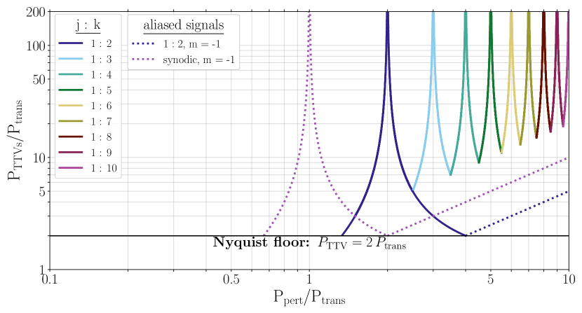
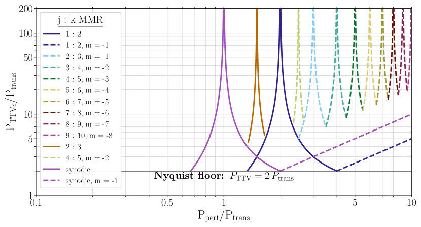
Figure 3: Analytic TTVs from super-period equation and their aliases for some $j:k$ near MMR TTVs for external perturbers. Also analytic TTVs from synodic period and its alias. [Top] $1:k$ super-periods shown. [Bottom] Aliases of first-order super-periods shown. Here we show how first-order super-periods can induce all the same TTV periods as higher order super-periods expected only for large eccentricities.

Let us start by focusing on an external perturbing planet. We define $P_{\mathrm{pert}}$ as the period of the perturbing planet and $P_{\mathrm{trans}}$ as the period of the transiting planet. Since for near MMR TTVs $P_{\mathrm{trans}}/P_{\mathrm{pert}}\sim j/k$, we can solve for the nearest $k$ given some $j$ and the period ratio $P_{\mathrm{pert}}/P_{\mathrm{trans}}$, via

$$k=\mathrm{round}(j\,[\,P_{\mathrm{pert}}/P_{\mathrm{trans}}])$$ (10)

Assuming $j$ is 1, we can plot all $1:k$ super-periods for external perturbers with period ratios $1.5<P_{\mathrm{pert}}/P_{\mathrm{trans}}<10$. This is shown in Figure 3.

As stated earlier, first-order super-periods are expected to dominate near-resonant TTVs in the low-eccentricity regime. Thus, for nearly circular orbits, we wouldn’t expect $j:k=1:k$ for $k>1$ to be frequently detected in TTV data. Thus, we also plot the alias of the $1:2$ in this complete parameter space. Additionally we plot the synodic TTV and its alias in this complete parameter space. We find that only a solution of $m=-1$ provides an observable solution (i.e., aliased period larger than the Nyquist period), for both the synodic and the $1:2$ MMR in this period ratio regime. Interestingly, we find that the alias of the synodic period is equal to the period of the perturbing planet for period ratios larger than 2 and that the alias of the $1:2$ super-period is equal to half the period of the perturbing planet for period ratios larger than 4. For more discussion on what we dub the “exoplanet edge” see Section 4.2. These aliases are also shown in Figure 3.

We then investigated other first-order super-periods, and find that for an external perturber with a super-period peak induced by the $j:k$ MMR (where $k>j$), you recover the same super-period peak from the $m=-[k-j-1]$ alias of the $k-1:k$ MMR. We show this in Figure 3. We also plot the super-period from $j:k=2:3$ and its $m=-2$ alias.

3.2 Internal Perturber

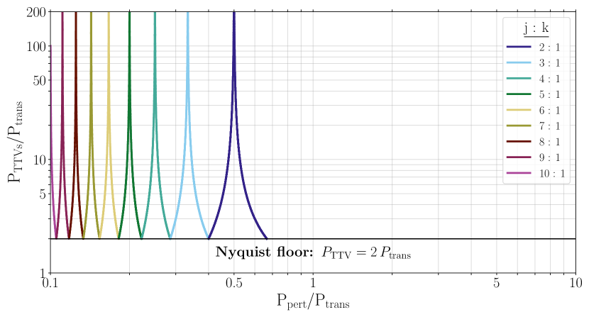
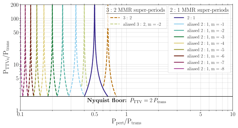
Figure 4: Analytic TTVs from super-period equation and their aliases for some $j:k$ near MMR TTVs for internal perturbers. [Top] $1:k$ super-periods shown. [Bottom] Aliases of first-order super-periods shown. Here we show how first-order super-periods can induce all the same TTV periods as higher order super-periods expected only for large eccentricities.

Now we turn to internal perturbers. Similarly to the external perturber case, we can use the fact that for MMR TTVs $P_{\mathrm{trans}}/P_{\mathrm{pert}}\sim j/k$, to solve for the nearest $j$ given some $k$ and the period ratio $P_{\mathrm{pert}}/P_{\mathrm{trans}}$, via

$$j=\mathrm{round}(k/[\,P_{\mathrm{pert}}/P_{\mathrm{trans}}])$$ (11)

Assuming $k$ is 1, we can plot all $j:1$ super-periods for internal perturbers with period ratios $0.1<P_{\mathrm{pert}}/P_{\mathrm{trans}}<1/1.25$. This is shown in Figure 4.

Again, in the low-eccentricity regime, we expect first-order resonant TTVs to be the dominant signal – so let’s determine the aliases for the $1:2$ super-period. Similarly to the external perturbers, we find that we can explain the peaks with first-order super-periods and their aliases. Here, we find that the $m=-[j-k-1]$ alias of the $2:1$ super-period are exactly equal to the nearest $j:k$ super-period when orbital period ratios are in the range with period ratios $0.1<P_{\mathrm{pert}}/P_{\mathrm{trans}}<1/1.25$. This is shown in Figure 4. We repeat this process for the $3:2$ MMR and plot its resulting super-period and one of its aliases in Figure 4.

3.3 Chaotic Region

As presented in Deck et al. (2013), first-order resonances become chaotic and thus unstable for close two-planet systems. Specifically, they show that if $\epsilon_{p}$ is equal to the sum of the masses of the planets in units of the star’s mass, then all orbits should be chaotic if their averaged period ratio satisfies

$$P_{2}/P_{1}\lesssim 1+2.2\epsilon_{p}^{2/7}.$$ (12)

This criterion is presented as the minimum criterion for widespread chaos – as this neglects the effect of higher order resonances. Therefore, planets with period ratios internal to this regime, chaotic orbits are expected as overlapping first-order resonances cause changes in the semi-major axes significant enough to oscillate the TTVs between neighboring resonances. Our model comparison approach only works when we can set priors that distinguish near-resonant periods that will not cause these oscillations. Around a Solar mass star, plugging in two Earth mass planets, this corresponds to period ratios of $\sim$1.07 and plugging in two Jupiter mass planets corresponds to period ratios of $\sim$1.4.

4 Discussion

4.1 Combining the Analytic and Numerical Solutions

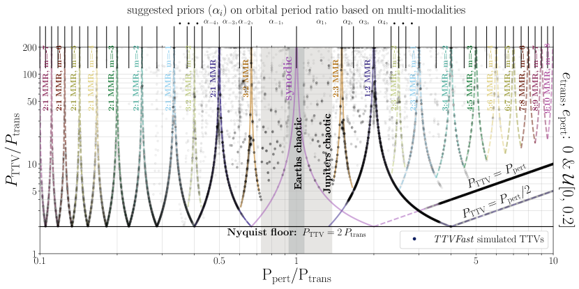
Figure 5: Analytic and numerical results for TTV period vs. orbital period ratio space of planet-planet TTVs. The analytic model, explained solely by first-order mean-motion resonant super periods and the synodic period (and their aliases), fits the numerical results very well. Numerical simulations combine all observable TTVs that passed tests explained in Figure 1. We also show the chaotic boundaries as defined by Deck et al. (2013) for two Earth mass and two Jupiter mass planets, respectively, around a Solar mass star. Also recommended orbital period ratio prior boundaries for efficient and accurate modeling.

We can now bring everything together – incorporating the effects of both internal and external perturbers and mapping the chaotic region as defined by Deck et al. (2013). We can additionally include the numerical simulations to investigate how well our analytic expression describes the numerical simulations. This can be seen in Figure 5 and the strength of the fit is apparent. This suggests that unsurprisingly, the dominant signal in nearly circular planet-planet TTVs are well described by the analytic first-order MMR super-periods (and their aliases) explained in Section 3.

There are some anomalous TTVs, that do not fall on the analytically expressed peaks – more significantly the closer you get in orbital period ratio space. These are likely other aliases of first-order super-periods. However, as the vast majority of TTV signals fall along our analytic solutions, we can use these to define efficient priors for modeling TTVs from perturbing planets.

From an analytic standing, we now have a sense of where the multi-modalities are likely to arise in period ratio space. One could imagine that when a TTV is observed, in characterizing the perturbing planets orbital characteristics, we essentially would start by drawing a horizontal line across Figure 5 and then any intersection would be a possible period ratio solution. In practice, this would be done typically with a numerical simulator and some type of sampling model (e.g., MCMC or nest sampling). However, as previously stated, adopting a wide prior on perturber period, will result in a posterior that tends to get stuck in one of the orbital period modes.

One would thus want to define uniform priors that span from the peak in TTV period space to the valley where another super-period takes over as the dominant effect. That is, to test orbital period ratios ranging from 1/10 to 10, one should adopt uniform priors spanning the orbital period ratio ranges corresponding to the first-order super-periods, as shown in Table 1

Prior Name	Period Ratio Range	$j:k$ Super-Period
$\alpha_{-21}$	$\mathcal{U}\left[\frac{1}{10},\,\frac{2}{19}\right]$	$2:1$, $m=-8$
$\alpha_{-20}$	$\mathcal{U}\left[\frac{2}{19},\,\frac{1}{9}\right]$	$2:1$, $m=-7$
$\alpha_{-19}$	$\mathcal{U}\left[\frac{1}{9},\,\frac{2}{17}\right]$	$2:1$, $m=-7$
$\alpha_{-18}$	$\mathcal{U}\left[\frac{2}{17},\,\frac{1}{8}\right]$	$2:1$, $m=-6$
$\alpha_{-17}$	$\mathcal{U}\left[\frac{1}{8},\,\frac{2}{15}\right]$	$2:1$, $m=-6$
$\alpha_{-16}$	$\mathcal{U}\left[\frac{2}{15},\,\frac{1}{7}\right]$	$2:1$, $m=-5$
$\alpha_{-15}$	$\mathcal{U}\left[\frac{1}{7},\,\frac{2}{13}\right]$	$2:1$, $m=-5$
$\alpha_{-14}$	$\mathcal{U}\left[\frac{2}{13},\,\frac{1}{6}\right]$	$2:1$, $m=-4$
$\alpha_{-13}$	$\mathcal{U}\left[\frac{1}{6},\,\frac{2}{11}\right]$	$2:1$, $m=-4$
$\alpha_{-12}$	$\mathcal{U}\left[\frac{2}{11},\,\frac{1}{5}\right]$	$2:1$, $m=-3$
$\alpha_{-11}$	$\mathcal{U}\left[\frac{1}{5},\,\frac{2}{9}\right]$	$2:1$, $m=-3$
$\alpha_{-10}$	$\mathcal{U}\left[\frac{2}{9},\,\frac{1}{4}\right]$	$2:1$, $m=-2$
$\alpha_{-9}$	$\mathcal{U}\left[\frac{1}{4},\,\frac{2}{7}\right]$	$2:1$, $m=-2$
$\alpha_{-8}$	$\mathcal{U}\left[\frac{2}{7},\,\frac{1}{3}\right]$	$2:1$, $m=-1$
$\alpha_{-7}$	$\mathcal{U}\left[\frac{1}{3},\,\frac{3}{8}\right]$	$2:1$, $m=-1$
$\alpha_{-6}$	$\mathcal{U}\left[\frac{3}{8},\,\frac{2}{5}\right]$	$3:2$, $m=-2$
$\alpha_{-5}$	$\mathcal{U}\left[\frac{2}{5},\,\frac{3}{7}\right]$	$3:2$, $m=-2$
$\alpha_{-4}$	$\mathcal{U}\left[\frac{3}{7},\,\frac{1}{2}\right]$	$2:1$
$\alpha_{-3}$	$\mathcal{U}\left[\frac{1}{2},\,\frac{3}{5}\right]$	$2:1$
$\alpha_{-2}$	$\mathcal{U}\left[\frac{3}{5},\,\frac{2}{3}\right]$	$3:2$
$\alpha_{-1}$	$\mathcal{U}\left[\frac{2}{3},\,1\right]$	$3:2$
$\alpha_{1}$	$\mathcal{U}\left[1,\,\frac{3}{2}\right]$	$2:3$
$\alpha_{2}$	$\mathcal{U}\left[\frac{3}{2},\,\frac{5}{3}\right]$	$2:3$
$\alpha_{3}$	$\mathcal{U}\left[\frac{5}{3},\,2\right]$	$1:2$
$\alpha_{4}$	$\mathcal{U}\left[2,\,\frac{7}{3}\right]$	$1:2$
$\alpha_{5}$	$\mathcal{U}\left[\frac{7}{3},\,\frac{5}{2}\right]$	$2:3$, $m=-2$
$\alpha_{6}$	$\mathcal{U}\left[\frac{5}{2},\,\frac{8}{3}\right]$	$2:3$, $m=-2$
$\alpha_{7}$	$\mathcal{U}\left[\frac{8}{3},\,3\right]$	$2:3$, $m=-1$
$\alpha_{8}$	$\mathcal{U}\left[3,\,\frac{7}{2}\right]$	$2:3$, $m=-1$
$\alpha_{9}$	$\mathcal{U}\left[\frac{7}{2},\,4\right]$	$3:4$, $m=-2$
$\alpha_{10}$	$\mathcal{U}\left[4,\,\frac{9}{2}\right]$	$3:4$, $m=-2$
$\alpha_{11}$	$\mathcal{U}\left[\frac{9}{2},\,5\right]$	$4:5$, $m=-3$
$\alpha_{12}$	$\mathcal{U}\left[5,\,\frac{11}{2}\right]$	$4:5$, $m=-3$
$\alpha_{13}$	$\mathcal{U}\left[\frac{11}{2},6\right]$	$5:6$, $m=-4$
$\alpha_{14}$	$\mathcal{U}\left[6,\,\frac{13}{2}\right]$	$5:6$, $m=-4$
$\alpha_{15}$	$\mathcal{U}\left[\frac{13}{2},7\right]$	$6:7$, $m=-5$
$\alpha_{16}$	$\mathcal{U}\left[7,\,\frac{15}{2}\right]$	$6:7$, $m=-5$
$\alpha_{17}$	$\mathcal{U}\left[\frac{15}{2},8\right]$	$7:8$, $m=-6$
$\alpha_{18}$	$\mathcal{U}\left[8,\,\frac{17}{2}\right]$	$7:8$, $m=-6$
$\alpha_{19}$	$\mathcal{U}\left[\frac{17}{2},9\right]$	$8:9$, $m=-7$
$\alpha_{20}$	$\mathcal{U}\left[9,\,\frac{19}{2}\right]$	$8:9$, $m=-7$
$\alpha_{21}$	$\mathcal{U}\left[\frac{19}{2},10\right]$	$9:10$, $m=-8$

Table 1: Prior names, orbital period range that each prior spans, and the corresponding super-period that analytically explains this mode of the unseen perturbing planet’s period. Here, $\alpha_{i}=\mathrm{P}(\bm{\theta}|\mathcal{M}_{i})$, the local prior on free parameters.

These period ranges can also be seen in Figure 5. By sampling the TTV inversion problem in these period ranges, we can avoid the multi-modality otherwise expected in single-planet TTVs, in each period range there should only one solution. Given this set of prior ranges, motivated by both numerical and analytic solutions, one could then (i) calculate the model evidence of a perturbing planet solution in a single prior range and (ii) correctly sample the full posterior distribution of perturbing planet properties, combining each individual posterior using Bayesian model averaging and using the individual evidences as weights.

4.2 The Exoplanet Edge

There is one anomalous effect besides the otherwise super-period “peak” dominated orbital landscape: the two “edges” found at orbital period ratios $\geq$ 4. As shown in Figure 5, the TTV periods of these two edges are equal to the period of the perturbing planet and half the period of the perturbing planet. Interestingly, we find that TTVs are not observed with periods faster than half the orbital period of the perturbing planet.

Thus, in addition to shedding light in the multi-modality of low-eccentricity single planet systems with TTVs, these analytic and numerical simulations reveal another effect – a minimum recoverable TTV for external perturbers with periods. This limiting “exoplanet edge” for planet-planet TTVs is discussed in depth in Yahalomi et al. (2024a), where they also show that the exoplanet edge persists for high eccentricity systems.

5 Parameter Estimation and Model Selection

We now turn to the problem of how to fit the TTVs of a transiting planet (with no other known companions) that exhibits TTVs. First, we highlight that simply throwing an MCMC or nested sampling algorithm at the data with very broad priors is problematic. The modes are too numerous (infinite in fact), too densely packed and too sharp for algorithms to reliably recover them. If modes are missed, not only are the posteriors inaccurate but so too is the model evidence - which is crucial if one wishes to rank competing models (e.g. an exomoon). These problems are so extreme that they have largely prevented the community from inferring landscape of allowed perturbing planet solutions to date.

As an aside, one might question the point of even attempting this. After all, even a correctly sampled posterior will inevitably be highly multi-modal still. It is unlikely we will arrive at a unique solution, except in rare cases like KOI-872 which exhibit outstanding signal-to-noise (Nesvorný et al., 2012). But a multi-modal posterior is still useful, constraining the global architecture of the system, especially when combined with other measurements such as radial velocities or astrometry. Further, the Bayesian evidence can at last be correctly estimated, allowing one to weigh different models. But perhaps the most important argument is this - there are thousands of such systems and we will likely find many, many more in the years and decades ahead. Each example is a signal, a whisper of that particular system’s configuration. Combined together, they become a chorus speaking to us about the demographics of exoplanets more broadly.

5.1 Sampling the Global Posterior

The key to making progress is to leverage the map revealed in this work. With the $N$ appropriate period priors now established, one could then run $N$ fits in each window. In each fit, one would follow the standard process regressing a TTV model to the data, but the prior on the perturbing planet’s period would be bounded by one of perturbing period commensurable with the first-order MMR modes. The global posterior is then found by combining these local solutions via Bayesian model averaging.

Consider that from each local fit, we have a unique prior on the free parameters, $\bm{\theta}$, defined as $\mathrm{P}(\bm{\theta}|\mathcal{M}_{i})$, where $\mathcal{M}_{i}$ denotes the conditional of adopting the model that uses the $i^{\mathrm{th}}$ window. Further, we obtain a local posterior distribution on $\bm{\theta}$ from each fit defined as $\mathrm{P}(\bm{\theta}|\mathcal{D},\mathcal{M}_{i})$, where $\mathcal{D}$ represents the transit timing data (common to all models). The local posterior can be defined via Bayes’ theorem as:

$$\underbrace{\mathrm{P}(\bm{\theta}|\mathcal{D},\mathcal{M}_{i})}_{\shortstack{\scriptsize$\mathrm{local}\,\,\bm{\theta}$\\ \scriptsize$\mathrm{posterior}$}}=\frac{\overbrace{\mathrm{P}(\mathcal{D}|\bm{\theta},\mathcal{M}_{i})}^{\shortstack{\scriptsize$\mathrm{local}\,\,\bm{\theta}$ \\ \scriptsize$\mathrm{evidence}$}}\overbrace{\mathrm{P}(\bm{\theta}|\mathcal{M}_{i})}^{\shortstack{\scriptsize$\mathrm{local}\,\,\bm{\theta}$ \\ \scriptsize$\mathrm{prior}$}}}{\underbrace{\mathrm{P}(\mathcal{D}|\mathcal{M}_{i})}_{\shortstack{\scriptsize$\mathrm{local\,\,model}$ \\ \scriptsize$\mathrm{evidence}$}}}.$$ (13)

The global posterior can now be found by performing a weighted sum of each posterior, with the weights set by the probability of each model, given the data:

$$\underbrace{\mathrm{P}(\bm{\theta}|\mathcal{D})}_{\shortstack{\scriptsize$\mathrm{global}\,\,\bm{\theta}$ \\ \scriptsize$\mathrm{posterior}$}}=\displaystyle\sum_{i=1}^{N}\underbrace{\mathrm{P}(\bm{\theta}|\mathcal{D},\mathcal{M}_{i})}_{\shortstack{\scriptsize$\mathrm{local}\,\,\bm{\theta}$ \\ \scriptsize$\mathrm{posterior}$}}\underbrace{\mathrm{P}(\mathcal{M}_{i}|\mathcal{D})}_{\shortstack{\scriptsize$\mathrm{local\,\,model}$ \\ \scriptsize$\mathrm{posterior}$}}.$$ (14)

In the above, the weights, $\mathrm{P}(\mathcal{M}_{i}|\mathcal{D})$, should not be confused with the Bayesian evidences, $\mathrm{P}(\mathcal{D}|\mathcal{M}_{i})$. However they are intimately related via Bayes’ theorem as

$$\underbrace{\mathrm{P}(\mathcal{M}_{i}|\mathcal{D})}_{\shortstack{\scriptsize$\mathrm{local\,\,model}$ \\ \scriptsize$\mathrm{posterior}$}}=\frac{\overbrace{\mathrm{P}(\mathcal{D}|\mathcal{M}_{i})}^{\shortstack{\scriptsize$\mathrm{local\,\,model}$ \\ \scriptsize$\mathrm{evidence}$}}\overbrace{\mathrm{P}(\mathcal{M}_{i})}^{\shortstack{\scriptsize$\mathrm{local\,\,model}$ \\ \scriptsize$\mathrm{prior}$}}}{\underbrace{\mathrm{P}(\mathcal{D})}_{\shortstack{\scriptsize$\mathrm{global\,\,model}$ \\ \scriptsize$\mathrm{evidence}$}}}.$$ (15)

The above is useful since it allows one to inject demographics priors into the inference. For example, based on previous exoplanet demographics studies, one might wish to down-weight certain windows where planets are rare, which can be achieved using $\mathrm{P}(\mathcal{M}_{i})$. Finally, to complete the procedure, we need to evaluate $\mathrm{P}(\mathcal{D})$. Since this term acts like a normalization constant, it can be found by the demand for all probabilities to sum to unity, such that

$$\underbrace{\mathrm{P}(\mathcal{D})}_{\shortstack{\scriptsize$\mathrm{global\,\,model}$ \\ \scriptsize$\mathrm{evidence}$}}=\displaystyle\sum_{j=1}^{N}\underbrace{\mathrm{P}(\mathcal{D}|\mathcal{M}_{j})}_{\shortstack{\scriptsize$\mathrm{local\,\,model}$ \\ \scriptsize$\mathrm{evidence}$}}\underbrace{\mathrm{P}(\mathcal{M}_{j})}_{\shortstack{\scriptsize$\mathrm{local\,\,model}$ \\ \scriptsize$\mathrm{prior}$}}.$$ (16)

As a final note, one might be concerned that our defined windows do not guarantee a uni-modal solution, since for example one of our assumptions is low-eccentricity. Accordingly, the use of a multi-modal fitting algorithm is still advised, to account for this possibility. Nevertheless, the number of modes will be far more manageable in these bite-size windows that the entire parameter volume and lead to far more reliable results.

5.2 Planets vs. Moons

At this point, it’s fairly straight-forward to extend our results to compare the assumed perturbing planet model to some other model, for example an exomoon as being responsible for the TTVs. It should be noted in the last subsection, all of the probability distributions are implicitly conditional upon the global model - a perturbing planet. Thus really one should adjust $\mathrm{P}(\mathcal{D})\to\mathrm{P}(\mathcal{D}|\mathrm{PP})$ where “PP” denotes perturbing planet. Thus, Equation 16 provides the overall evidence of the PP model.

The user now need only execute an additional fit for the moon model(s), which we dub “PM”. The odds ratio between the two models will then by given as

$$\frac{\mathrm{P}(\mathrm{PP}|\mathcal{D})}{\mathrm{P}(\mathrm{PM}|\mathcal{D})}=\frac{\mathrm{P}(\mathcal{D}|\mathrm{PP})}{\mathrm{P}(\mathcal{D}|\mathrm{PM})}\frac{\mathrm{P}(\mathrm{PP})}{\mathrm{P}(\mathrm{PM})}$$ (17)

The ratio of the model priors is particularly challenging to estimate given the dearth of exomoon detections, and thus practically speaking setting this ratio to unity - equivalent to a Bayes factor - would be a possible path forward.

6 Conclusion

Transit timing variations (TTVs) are found in many transiting planet systems. When uncovered in (ostensibly) single-planet systems, the TTVs induced by a perturbing (non-transiting) planet are difficult to characterize – as the solution is highly multi-modal with respect to the unseen planet’s orbital period.

As multi-planet systems have been found to date to generally have low eccentricities, we adopt a pragmatic approach and study the orbital landscape of nearly circular planet-planet TTVs. This eccentricity space has the advantage of being dominated by first-order super-periods, allowing for us to analytically map out the location of these multi-modalities in orbital period ratio space.

Analytic formulae of first-order super-periods and their aliases, as well as numerical ($N$-body) simulations reveal that there are quantifiable modes in orbital period ratio space commensurable with a given TTV period. Therefore, in order to efficiently and accurately sample the complete parameter space of possible perturbing planets responsible for TTVs observed in single-planet systems, one must adopt priors informed by these super-periods and their aliases. We provide a set of orbital period ratios for which period priors should be defined. We then demonstrate how one could use these priors in order to effectively sample the complete parameter space for perturbing planets, and then adopt a Bayesian model comparison approach to determine whether a TTV signal is more likely cause by an unseen perturbing planet or an unseen perturbing moon. In a future work, we will test this model comparison approach via injection recovery of planet-planet systems and planet-moon systems.

Additionally, we uncover that perturbing planets don’t induce observable TTVs with a dominant period faster than half their own orbital period. As a result, TTVs observed with period faster than this limiting “exoplanet edge” are suggestive of additional mass in the system – thus providing a new path to uncovering new exoplanets and perhaps exomoons. For more on this, see Yahalomi et al. (2024a).

References

- Agol & Deck (2016) Agol, E., & Deck, K. 2016, The Astrophysical Journal, 818, 177, doi: 10.3847/0004-637x/818/2/177
- Agol & Fabrycky (2018) Agol, E., & Fabrycky, D. C. 2018, in Handbook of Exoplanets, ed. H. J. Deeg & J. A. Belmonte, 7, doi: 10.1007/978-3-319-55333-7_7
- Agol et al. (2005) Agol, E., Steffen, J., Sari, R., & Clarkson, W. 2005, MNRAS, 359, 567, doi: 10.1111/j.1365-2966.2005.08922.x
- Agol et al. (2021) Agol, E., Dorn, C., Grimm, S. L., et al. 2021, The Planetary Science Journal, 2, 1, doi: 10.3847/PSJ/abd022
- Awiphan & Kerins (2013) Awiphan, S., & Kerins, E. 2013, MNRAS, 432, 2549, doi: 10.1093/mnras/stt614
- Dawson & Fabrycky (2010) Dawson, R. I., & Fabrycky, D. C. 2010, The Astrophysical Journal, 722, 937, doi: 10.1088/0004-637x/722/1/937
- Deck & Agol (2015) Deck, K. M., & Agol, E. 2015, ApJ, 802, 116, doi: 10.1088/0004-637X/802/2/116
- Deck & Agol (2016) —. 2016, ApJ, 821, 96, doi: 10.3847/0004-637X/821/2/96
- Deck et al. (2014) Deck, K. M., Agol, E., Holman, M. J., & Nesvorný, D. 2014, ApJ, 787, 132, doi: 10.1088/0004-637X/787/2/132
- Deck et al. (2013) Deck, K. M., Payne, M., & Holman, M. J. 2013, ApJ, 774, 129, doi: 10.1088/0004-637X/774/2/129
- Dobrovolskis & Borucki (1996) Dobrovolskis, A. R., & Borucki, W. J. 1996, in Bulletin of the American Astronomical Society, Vol. 28, 1112
- Fabrycky et al. (2014) Fabrycky, D. C., Lissauer, J. J., Ragozzine, D., et al. 2014, ApJ, 790, 146, doi: 10.1088/0004-637X/790/2/146
- Figueira et al. (2012) Figueira, P., Marmier, M., Boué, G., et al. 2012, A&A, 541, A139, doi: 10.1051/0004-6361/201219017
- Hadden & Lithwick (2014) Hadden, S., & Lithwick, Y. 2014, ApJ, 787, 80, doi: 10.1088/0004-637X/787/1/80
- Hadden & Lithwick (2016) —. 2016, ApJ, 828, 44, doi: 10.3847/0004-637X/828/1/44
- Hadden & Lithwick (2018) Hadden, S., & Lithwick, Y. 2018, The Astronomical Journal, 156, 95, doi: 10.3847/1538-3881/aad32c
- Heller (2014) Heller, R. 2014, ApJ, 787, 14, doi: 10.1088/0004-637X/787/1/14
- Heller et al. (2016) Heller, R., Hippke, M., Placek, B., Angerhausen, D., & Agol, E. 2016, A&A, 591, A67, doi: 10.1051/0004-6361/201628573
- Holczer et al. (2015) Holczer, T., Shporer, A., Mazeh, T., et al. 2015, The Astrophysical Journal, 807, 170, doi: 10.1088/0004-637x/807/2/170
- Holman & Murray (2005) Holman, M. J., & Murray, N. W. 2005, Science, 307, 1288, doi: 10.1126/science.1107822
- Holman et al. (2010) Holman, M. J., Fabrycky, D. C., Ragozzine, D., et al. 2010, Science, 330, 51, doi: 10.1126/science.1195778
- Hunter (2007) Hunter, J. D. 2007, Computing in Science and Engineering, 9, 90, doi: 10.1109/MCSE.2007.55
- Ioannidis et al. (2016) Ioannidis, P., Huber, K. F., & Schmitt, J. H. M. M. 2016, A&A, 585, A72, doi: 10.1051/0004-6361/201527184
- Jones et al. (2001) Jones, E., Oliphant, T., Peterson, P., et al. 2001, SciPy: Open source scientific tools for Python. http://www.scipy.org/
- Kipping (2021) Kipping, D. 2021, MNRAS, 500, 1851, doi: 10.1093/mnras/staa3398
- Kipping & Teachey (2020) Kipping, D., & Teachey, A. 2020, Serbian Astronomical Journal, 201, 25, doi: 10.2298/SAJ2001025K
- Kipping & Yahalomi (2022) Kipping, D., & Yahalomi, D. A. 2022, Monthly Notices of the Royal Astronomical Society, 518, 3482, doi: 10.1093/mnras/stac3360
- Kipping (2009a) Kipping, D. M. 2009a, MNRAS, 392, 181, doi: 10.1111/j.1365-2966.2008.13999.x
- Kipping (2009b) —. 2009b, MNRAS, 396, 1797, doi: 10.1111/j.1365-2966.2009.14869.x
- Kipping et al. (2009) Kipping, D. M., Fossey, S. J., & Campanella, G. 2009, MNRAS, 400, 398, doi: 10.1111/j.1365-2966.2009.15472.x
- Lithwick et al. (2012) Lithwick, Y., Xie, J., & Wu, Y. 2012, ApJ, 761, 122, doi: 10.1088/0004-637X/761/2/122
- Lomb (1976) Lomb, N. R. 1976, Ap&SS, 39, 447, doi: 10.1007/BF00648343
- Mazeh et al. (2015) Mazeh, T., Holczer, T., & Shporer, A. 2015, ApJ, 800, 142, doi: 10.1088/0004-637X/800/2/142
- Mazeh et al. (2013) Mazeh, T., Nachmani, G., Holczer, T., et al. 2013, ApJS, 208, 16, doi: 10.1088/0067-0049/208/2/16
- McClellan et al. (1998) McClellan, J. H., Schafer, R. W., & Yoder, M. A. 1998, DSP First: A multimedia approach (Prentice-Hall)
- Meschiari & Laughlin (2010) Meschiari, S., & Laughlin, G. P. 2010, ApJ, 718, 543, doi: 10.1088/0004-637X/718/1/543
- Miralda-Escudé (2002) Miralda-Escudé, J. 2002, ApJ, 564, 1019, doi: 10.1086/324279
- Murray & Dermott (1999) Murray, C. D., & Dermott, S. F. 1999, Solar System Dynamics, doi: 10.1017/CBO9781139174817
- Nesvorný (2009) Nesvorný, D. 2009, ApJ, 701, 1116, doi: 10.1088/0004-637X/701/2/1116
- Nesvorný & Beaugé (2010) Nesvorný, D., & Beaugé, C. 2010, ApJ, 709, L44, doi: 10.1088/2041-8205/709/1/L44
- Nesvorný et al. (2013) Nesvorný, D., Kipping, D., Terrell, D., et al. 2013, ApJ, 777, 3, doi: 10.1088/0004-637X/777/1/3
- Nesvorný et al. (2012) Nesvorný, D., Kipping, D. M., Buchhave, L. A., et al. 2012, Science, 336, 1133, doi: 10.1126/science.1221141
- Nesvorný & Morbidelli (2008) Nesvorný, D., & Morbidelli, A. 2008, ApJ, 688, 636, doi: 10.1086/592230
- Nesvorný & Vokrouhlický (2014) Nesvorný, D., & Vokrouhlický, D. 2014, ApJ, 790, 58, doi: 10.1088/0004-637X/790/1/58
- Nyquist (1928) Nyquist, H. 1928, Transactions of the American Institute of Electrical Engineers, 47, 617, doi: 10.1109/T-AIEE.1928.5055024
- Oshagh et al. (2013) Oshagh, M., Santos, N. C., Boisse, I., et al. 2013, A&A, 556, A19, doi: 10.1051/0004-6361/201321309
- Petit et al. (2018) Petit, A. C., Laskar, J., & Boué, G. 2018, A&A, 617, A93, doi: 10.1051/0004-6361/201833088
- Sanchis-Ojeda et al. (2011) Sanchis-Ojeda, R., Winn, J. N., Holman, M. J., et al. 2011, ApJ, 733, 127, doi: 10.1088/0004-637X/733/2/127
- Sartoretti & Schneider (1999) Sartoretti, P., & Schneider, J. 1999, A&AS, 134, 553, doi: 10.1051/aas:1999148
- Scargle (1982) Scargle, J. D. 1982, ApJ, 263, 835, doi: 10.1086/160554
- Schmitt et al. (2014) Schmitt, J. R., Agol, E., Deck, K. M., et al. 2014, ApJ, 795, 167, doi: 10.1088/0004-637X/795/2/167
- Shannon (1949) Shannon, C. 1949, Proceedings of the IRE, 37, 10, doi: 10.1109/JRPROC.1949.232969
- Siegel & Rogers (2022) Siegel, J. C., & Rogers, L. A. 2022, AJ, 164, 139, doi: 10.3847/1538-3881/ac8985
- Simon et al. (2007) Simon, A., Szatmáry, K., & Szabó, G. M. 2007, A&A, 470, 727, doi: 10.1051/0004-6361:20066560
- Steffen (2006) Steffen, J. H. 2006, Phd thesis, University of Washington
- Szabó et al. (2013) Szabó, R., Szabó, G. M., Dálya, G., et al. 2013, A&A, 553, A17, doi: 10.1051/0004-6361/201220132
- Tamayo et al. (2021) Tamayo, D., Murray, N., Tremaine, S., & Winn, J. 2021, The Astronomical Journal, 162, 220, doi: 10.3847/1538-3881/ac1c6a
- Tremaine & Dong (2012) Tremaine, S., & Dong, S. 2012, AJ, 143, 94, doi: 10.1088/0004-6256/143/4/94
- Van Eylen & Albrecht (2015) Van Eylen, V., & Albrecht, S. 2015, ApJ, 808, 126, doi: 10.1088/0004-637X/808/2/126
- VanderPlas (2018) VanderPlas, J. T. 2018, The Astrophysical Journal Supplement Series, 236, 16, doi: 10.3847/1538-4365/aab766
- Walt et al. (2011) Walt, S. v. d., Colbert, S. C., & Varoquaux, G. 2011, Computing in Science and Eng., 13, 22, doi: 10.1109/MCSE.2011.37
- Wisdom & Holman (1992) Wisdom, J., & Holman, M. 1992, AJ, 104, 2022, doi: 10.1086/116378
- Yahalomi et al. (2024a) Yahalomi, A. D., Kipping, D., Agol, E., & Nesvorný, D. 2024a, The Exoplanet Edge: Planets Don’t Induce Observable TTVs Faster than Half their Orbital Period
- Yahalomi et al. (2024b) Yahalomi, D. A., Kipping, D., Nesvorný, D., et al. 2024b, MNRAS, 527, 620, doi: 10.1093/mnras/stad3070