MARS: Unleashing the Power of Variance Reduction for Training Large Models

Abstract

Training deep neural networks—and more recently, large models—demands efficient and scalable optimizers. Adaptive gradient algorithms like Adam, AdamW, and their variants have been central to this task. Despite the development of numerous variance reduction algorithms in the past decade aimed at accelerating stochastic optimization in both convex and nonconvex settings, variance reduction has not found widespread success in training deep neural networks or large language models. Consequently, it has remained a less favored approach in modern AI. In this paper, to unleash the power of variance reduction for efficient training of large models, we propose a unified optimization framework, MARS (Make vAriance Reduction Shine), which reconciles preconditioned gradient methods with variance reduction via a scaled stochastic recursive momentum technique. Within our framework, we introduce three instances of MARS that leverage preconditioned gradient updates based on AdamW, Lion, and Shampoo, respectively. We also draw a connection between our algorithms and existing optimizers. Experimental results on training GPT-2 models indicate that MARS consistently outperforms AdamW by a large margin.

1 Introduction

Adaptive gradient methods such as Adam (Kingma, 2014) and AdamW (Loshchilov, 2017) have become the predominant optimization algorithms in deep learning. With the surge of large language models, the majority of the renowned models, including GPT-2 (Radford et al., 2019), GPT-3 (Brown, 2020), PaLM (Chowdhery et al., 2023) and Llama 3 (Dubey et al., 2024) are trained with adaptive gradient methods. Numerous efforts have been made to improve adaptive gradient methods from both first-order and second-order optimization perspectives. For example, You et al. (2019) introduced LAMB, a layerwise adaptation technique that boosts training efficiency for BERT (Devlin, 2018). Using symbolic search, Chen et al. (2023) developed Lion, achieving faster training and reduced memory usage. Liu et al. (2023) designed Sophia, leveraging stochastic diagonal Hessian estimators to accelerate training. Gupta et al. (2018) proposed Shampoo, which performs stochastic optimization over tensor spaces with preconditioning matrices for each dimension. Anil et al. (2020) further refined Shampoo to give a scalable, practical version. Recently, Vyas et al. (2024) showed that Shampoo is equivalent to Adafactor (Shazeer and Stern, 2018) in the eigenbasis of Shampoo’s preconditioner, and introduced SOAP, which stabilizes Shampoo with Adam. Importantly, recent studies (Kaddour et al., 2024; Zhao et al., 2024) have shown that these optimizers perform on par with AdamW in LLM pretraining, yet do not outperform it. This suggests the ongoing challenge in developing adaptive gradient methods superior to Adam and AdamW for large-scale model training.

Since adaptive gradient methods face challenges of high stochastic gradient variance, and language model training inherently involves a high-variance optimization problem (McCandlish et al., 2018), it is natural to consider variance reduction techniques to address this challenge. There exists a large body of literature on variance reduction for stochastic optimization, such as SAG (Roux et al., 2012), SVRG (Johnson and Zhang, 2013) and STORM (Cutkosky and Orabona, 2019), which can improve the convergence of stochastic optimization. However, variance reduction has not found widespread success in training deep neural networks or large language models. Defazio and Bottou (2019) discussed why variance reduction can be ineffective in deep learning due to factors such as data augmentation, batch normalization, and dropout, which disrupt the finite-sum structure required by variance reduction principles. Nevertheless, in training language models, data augmentation, batch normalization, and dropout are nowadays rarely used, which opens the door for applying variance reduction techniques in optimizing these models. This naturally leads to the following research question:

Can variance reduction technique be applied to improve the performance of training large models?

In this paper, we answer the above question affirmatively by introducing a novel optimization framework called MARS (Make vAriance Reduction Shine), which incorporates variance reduction into adaptive gradient methods. Notably, we introduce a scaling parameter into the stochastic recursive momentum (STORM) (Cutkosky and Orabona, 2019) to adjust the strength of variance reduction and define a new gradient estimator. This gradient estimator undergoes gradient clipping and is subsequently subjected to exponential averaging. When the variance reduction strength is set to $1$, it recovers the vanilla STORM momentum. In addition, the second-order momentum update is defined by the reweighted intermediate variable. These together ensure optimization stability throughout the training process. We summarize our major contributions of this paper as follows:

• We propose a unified framework for preconditioned variance reduction, namely MARS. At its core, MARS comprises two major components: (1) a scaled stochastic recursive momentum, which provides a variance-reduced estimator of the full gradient for better gradient complexity; and (2) the preconditioned update, which approximates the second-order Newton’s method for better per-iteration complexity. By combining preconditioned gradient methods with variance reduction, MARS achieves the best of both worlds, accelerating the search for critical points in optimization.

• The MARS framework is versatile, accommodating all existing full matrix or diagonal Hessian approximations. Under this framework, we utilize three distinct designs of the preconditioning matrix, resulting in three specific instances of our MARS framework: MARS-AdamW, MARS-Lion, and MARS-Shampoo. Each variant demonstrates compatibility with their corresponding preconditioning in AdamW, Lion, and Shampoo, showing that MARS can seamlessly integrate with and do variance-reduction on these established methods.

• Empirically, we evaluated MARS-AdamW (or simply MARS) on GPT-2 fine-tuning tasks using the OpenWebText dataset. MARS demonstrated superior performance on GPT-2 large: it reached a validation loss of 2.58 within 27 billion tokens, whereas AdamW required 50 billion tokens to achieve the same level. The final validation loss achieved by MARS on GPT-2 large is 2.53, compared to 2.56 for AdamW. Furthermore, on the downstream task Hellaswag, MARS improved accuracy to 44.20%, outperforming AdamW’s 42.31% after training on 50 billion tokens, highlighting its superior performance in training large models.

Notations

In this paper, we assume $\mathbf{x}_{t}$ denotes the parameter of the language model at step $t$ and $\bm{\xi}_{1},...,\bm{\xi}_{T}\in\mathbf{\Xi}$ are a sequence of independent random variables which denote the training data for each step. For some objective function $f$ that is differentiable, we assume $\mathbb{E}[f(\mathbf{x},\bm{\xi}_{t})|\mathbf{x}]=F(\mathbf{x})$ for $\forall\mathbf{x},~{}\forall t$. In our algorithm, the training data of the current step $\bm{\xi}_{t}$ and previous step $\bm{\xi}_{t-1}$ are used for attaining different gradient for the same parameter $\mathbf{x}_{t}$, so we just explicitly indicate these variables for function $f$.

2 Preliminaries

In this section, we review the preliminaries of stochastic optimization, including standard stochastic gradient methods and variance reduction.

We consider minimizing an objective function $F(\cdot):\mathbb{R}^{d}\rightarrow\mathbb{R}$ as follows:

$$\min_{\mathbf{x}}F(\mathbf{x})=\mathbb{E}_{\bm{\xi}\sim\mathcal{D}}[f(\mathbf{x},\bm{\xi})],$$ (2.1)

where $f(\mathbf{x},\bm{\xi})$ is possibly nonconvex loss function, $\mathbf{x}\in\mathbb{R}^{d}$ is the optimization variable, $\bm{\xi}$ is a random vector (e.g., a training data point) drawn from an unknown data distribution $\mathcal{D}$. We assume the access to the first-order oracle, which returns an unbiased estimator of the gradient $\mathbb{E}[\nabla f(\mathbf{x},\bm{\xi})]=\nabla F(\mathbf{x})$. The standard stochastic gradient descent (SGD) algorithm yields:

$$\mathbf{x}_{t+1} =\mathbf{x}_{t}-\eta_{t}\nabla f(\mathbf{x}_{t},\bm{\xi}_{t}),$$ (2.2)

where $\eta_{t}>0$ is the learning rate or step size. SGD needs $\mathcal{O}(\varepsilon^{-4})$ stochastic gradient evaluations (i.e., gradient complexity or incremental first-order oracle complexity) to find a $\epsilon$-approximate first-order stationary points, i.e., $\|\nabla F(\mathbf{x})\|_{2}\leq\epsilon$ (Ghadimi and Lan, 2013).

To accelerate the convergence of SGD, variance reduction techniques have been extensively researched in both the machine learning and optimization communities over the past decade, resulting in numerous algorithms for convex optimization—such as SAG (Roux et al., 2012), SVRG (Johnson and Zhang, 2013), SAGA (Defazio et al., 2014), and SARAH (Nguyen et al., 2017a)—as well as for nonconvex optimization, including SVRG (Allen-Zhu and Yuan, 2016; Reddi et al., 2016), SNVRG (Zhou et al., 2020), SPIDER (Fang et al., 2018), and STORM (Cutkosky and Orabona, 2019), among others. Notably, for nonconvex optimization, SNVRG (Zhou et al., 2020), SPIDER (Fang et al., 2018) and STORM (Cutkosky and Orabona, 2019) can improve the gradient complexity of SGD from $\mathcal{O}(\varepsilon^{-4})$ to $\mathcal{O}(\varepsilon^{-3})$, demonstrating a provable advantage.

At the heart of variance reduction techniques is a variance-reduced stochastic gradient, exemplified by the method proposed by Johnson and Zhang (2013) as follows:

$$\mathbf{m}_{t}=\nabla f(\mathbf{x}_{t},\bm{\xi}_{t})-\nabla f(\widetilde{\mathbf{x}},\bm{\xi}_{t})+\nabla F(\widetilde{\mathbf{x}}),$$

where $\widetilde{\mathbf{x}}$ is an anchoring point (a.k.a., reference point) that updates periodically. This variance-reduced stochastic gradient can reduce the variance of the stochastic gradient by adding a correction term $-\nabla f(\widetilde{\mathbf{x}},\bm{\xi}_{t})+\nabla F(\widetilde{\mathbf{x}})$ based on a less frequently updated reference point $\widetilde{\mathbf{x}}$ and its full gradient $\nabla F(\widetilde{\mathbf{x}})$. It can be shown that the variance $\mathbf{m}_{t}$ can be controlled by $\|\mathbf{x}_{t}-\widetilde{\mathbf{x}}\|_{2}$, which will diminish as both $\mathbf{x}_{t}$ and $\widetilde{\mathbf{x}}$ converges to the stationary points when the algorithm makes progress. Subsequent improvements in variance reduction techniques were introduced in SARAH (Nguyen et al., 2017a) and SPIDER (Fang et al., 2018), which get rid of the anchor point and result in the following momentum update:

$$\mathbf{m}_{t} =\nabla f(\mathbf{x}_{t},\bm{\xi}_{t})-\nabla f(\mathbf{x}_{t-1},\bm{\xi}_{t})+\mathbf{m}_{t-1},$$

$$\mathbf{x}_{t+1} =\mathbf{x}_{t}-\eta_{t}\mathbf{m}_{t}.$$ (2.3)

In the context of training neural networks, $\mathbf{x}_{t}\in\mathbb{R}^{d}$ represents the trained weights in the neural network, $\bm{\xi}_{t}$ represents random data, and $\mathbf{m}_{t}$ is the variance-reduced (VR) first-order momentum. The stochastic gradient difference term $\nabla f(\mathbf{x}_{t},\bm{\xi}_{t})-\nabla f(\mathbf{x}_{t-1},\bm{\xi}_{t})$ cancels out common noise brought by $\bm{\xi}_{t}$, while pushing the gradient estimation from the estimator of $\nabla F(\mathbf{x}_{t-1})$ to the estimator of $\nabla F(\mathbf{x}_{t})$. However, $\mathbf{m}_{t}$ needs to be reset periodically to a full gradient (or a large batch stochastic gradient) $\nabla F(\mathbf{x}_{t})$, which we refer to as an anchoring step, analogous to the anchor point in SVRG.

Subsequently, Cutkosky and Orabona (2019) introduced Stochastic Recursive Momentum (STORM), a variant of standard momentum with an additional term, achieving the same convergence rate as SPIDER while eliminating the need for periodic anchoring:

$$\mathbf{m}_{t} =\beta_{1}\mathbf{m}_{t-1}+(1-\beta_{1})\nabla f(\mathbf{x}_{t},\bm{\xi}_{t})+\beta_{1}\big{(}\nabla f(\mathbf{x}_{t},\bm{\xi}_{t})-\nabla f(\mathbf{x}_{t-1},\bm{\xi}_{t})\big{)}$$ (2.4)

where $\beta_{1}>0$ is momentum parameter, and $\beta_{1}(\nabla f(\mathbf{x}_{t},\bm{\xi}_{t})-\nabla f(\mathbf{x}_{t-1},\bm{\xi}_{t}))$ is the additional term that has variance reduction effect. Note that if $\mathbf{x}_{t}\approx\mathbf{x}_{t-1}$, STORM becomes approximately the standard momentum.

Alternatively, (2.4) can be rewritten as an exponential moving average (EMA) of the first order momentum from previous step/iteration and the stochastic gradient with a gradient correction term:

$$\mathbf{m}_{t} =\beta_{1}\mathbf{m}_{t-1}+(1-\beta_{1})\Big{[}\nabla f(\mathbf{x}_{t},\bm{\xi}_{t})+\underbrace{\frac{\beta_{1}}{1-\beta_{1}}\big{(}\nabla f(\mathbf{x}_{t},\bm{\xi}_{t})-\nabla f(\mathbf{x}_{t-1},\bm{\xi}_{t})\big{)}}_{\text{gradient correction}}\Big{]}.$$ (2.5)

Theoretically, when assuming access to an unbiased stochastic first-order oracle to the objective function $F(\mathbf{x})$, STORM achieves the nearly optimal gradient complexity of $\mathcal{O}(\varepsilon^{-3})$ for non-convex and smooth optimization problems (Arjevani et al., 2023).

3 Method

In this section, we introduce MARS (Make vAriance Reduction Shine), a family of precondtioned optimization algorithms that perform variance reduction in gradient estimation.

3.1 MARS Framework

We first introduce our framework for a preconditioned, variance-reduced stochastic optimization, which unifies both first-order (e.g., AdamW, Lion) and second-order (e.g., Shampoo) adaptive gradient methods.

Preconditioned Variance Reduction.

Variance reduction methods achieve faster convergence than SGD, yet identifying optimal learning rates remains a practical challenge. Particularly, different parameters often exhibit varying curvatures, requiring tailored learning rates for each. One approach to addressing this issue is to use the Hessian matrix to precondition gradient updates, integrating curvature information into the updates. The idea stems from minimizing the second-order Taylor expansion at $\mathbf{x}_{t}$:

$$F(\mathbf{x}_{t+1})\approx F(\mathbf{x}_{t})+\nabla F(\mathbf{x}_{t})(\mathbf{x}_{t+1}-\mathbf{x}_{t})+\frac{1}{2}(\mathbf{x}_{t+1}-\mathbf{x}_{t})^{\top}\nabla^{2}F(\mathbf{x}_{t})(\mathbf{x}_{t+1}-\mathbf{x}_{t}),$$ (3.1)

resulting in the update formula $\mathbf{x}_{t+1}=\mathbf{x}_{t}-\mathbf{H}_{t}^{-1}\nabla F(\mathbf{x}_{t})$, where $\mathbf{H}_{t}:=\nabla^{2}F(\mathbf{x}_{t})\in\mathbb{R}^{d\times d}$ is the Hessian matrix. In our paper, we encapsulate the preconditioned gradient $\mathbf{H}_{t}^{-1}\nabla F(\mathbf{x}_{t})$ update within a more generalized framework of Online Mirror Descent (OMD) as in Gupta et al. (2018), leading to the following update rules:

$$\mathbf{x}_{t+1}=\arg\min_{\mathbf{x}\in\mathbb{R}^{d}}\bigg{\{}\eta_{t}\left\langle\mathbf{m}_{t},\mathbf{x}\right\rangle+\frac{1}{2}\|\mathbf{x}-\mathbf{x}_{t}\|_{\mathbf{H}_{t}}^{2}\bigg{\}},$$ (3.2)

where $\eta_{t}>0$ can be viewed as a base learning rate. Combining (3.2) with the STORM momentum, we obtain the following preconditioned variance-reduced update:

$$\mathbf{m}_{t} =\beta_{1}\mathbf{m}_{t-1}+(1-\beta_{1})\Big{[}\nabla f(\mathbf{x}_{t},\bm{\xi}_{t})+\frac{\beta_{1}}{1-\beta_{1}}\big{(}\nabla f(\mathbf{x}_{t},\bm{\xi}_{t})-\nabla f(\mathbf{x}_{t-1},\bm{\xi}_{t})\big{)}\Big{]},$$ (3.3)

$$\mathbf{x}_{t+1} =\arg\min_{\mathbf{x}\in\mathbb{R}^{d}}\bigg{\{}\eta_{t}\left\langle\mathbf{m}_{t},\mathbf{x}\right\rangle+\frac{1}{2}\|\mathbf{x}-\mathbf{x}_{t}\|_{\mathbf{H}_{t}}^{2}\bigg{\}}.$$ (3.4)

Remark 3.1.

SuperAdam (Huang et al., 2021) also incorporates the STORM into the design of adaptive gradient methods. However, their precondition matrix can be viewed as a special case of our general framework. SuperAdam’s design focuses on diagonal precondition matrix and draws heavily from the design used in Adam (Kingma, 2014), AdaGrad-Norm (Ward et al., 2020), and AdaBelief (Zhuang et al., 2020). Furthermore, their preconditioner matrix is designed following Adam’s structure but does not account for the revised definition of variance-reduced momentum, resulting in a significant mismatch between the first-order and second-order momentum. We will further clarify these differences when discussing specific instances of our framework.

Algorithm Design.

In practice, alongside our preconditioned variance-reduced update (3.3), we introduce a scaling parameter $\gamma_{t}$ to control the scale of gradient correction in variance reduction. We also introduce a new gradient estimator $\mathbf{c}_{t}$, which is the combination of stochastic gradient and the scaled gradient correction term:

$$\mathbf{c}_{t}=\nabla f(\mathbf{x}_{t},\bm{\xi}_{t})+\underbrace{{\color[rgb]{1,0,0}\gamma_{t}}\frac{\beta_{1}}{1-\beta_{1}}\big{(}\nabla f(\mathbf{x}_{t},\bm{\xi}_{t})-\nabla f(\mathbf{x}_{t-1},\bm{\xi}_{t})\big{)}}_{\text{scaled gradient correction}}.$$ (3.5)

When $\gamma_{t}=1$, (3.5) reduces to the second term of (3.3). On the other hand, when $\gamma_{t}=0$, (3.5) reduces to the stochastic gradient. Thus, $\mathbf{c}_{t}$ can be seen an gradient estimator with adjustable variance control. Following standard techniques in deep learning practice, we also perform gradient clipping on $\mathbf{c}_{t}$, which is calculated by:

$$\widetilde{\mathbf{c}}_{t}=\text{Clip}(\mathbf{c}_{t},1)=\begin{cases}\frac{\mathbf{c}_{t}}{\|\mathbf{c}_{t}\|_{2}}&\text{if }\|\mathbf{c}_{t}\|_{2}>1,\\ \mathbf{c}_{t}&\text{otherwise}.\end{cases}$$ (3.6)

We note that the Second-order Clipped Stochastic Optimization (Sophia) algorithm (Liu et al., 2023) also incorporates clipping in their algorithm design. However, their approach does clipping upon the preconditioned gradient with clipping-by-value, while our method applies clipping to the intermediate gradient estimate using the more standard technique of clipping-by-norm. After the gradient clipping, the VR momentum $\mathbf{m}_{t}$ can be calculated as the EMA of $\widetilde{\mathbf{c}}_{t}$. The resulting MARS algorithm is summarized in Algorithm 1.

Algorithm 1 MARS

1:  input: $\mathbf{x}_{0},\beta_{1},\{\gamma_{t}\},\{\eta_{t}\}$

2:  Set $\mathbf{m}_{0}\leftarrow\mathbf{0}$ and $\mathbf{x}_{1}\leftarrow\mathbf{x}_{0}$

3:  for $t=1,$ to $n$ do

4:     Sample $\bm{\xi}_{t}$ and let $\mathbf{c}_{t}=\nabla f(\mathbf{x}_{t},\bm{\xi}_{t})+\gamma_{t}\frac{\beta_{1}}{1-\beta_{1}}\big{(}\nabla f(\mathbf{x}_{t},\bm{\xi}_{t})-\nabla f(\mathbf{x}_{t-1},\bm{\xi}_{t})\big{)}$

5:     if $\|\mathbf{c}_{t}\|_{2}>1$, then $\tilde{\mathbf{c}}_{t}=\frac{\mathbf{c}_{t}}{\|\mathbf{c}_{t}\|_{2}}$ else $\widetilde{\mathbf{c}}_{t}=\mathbf{c}_{t}$

6:     $\mathbf{m}_{t}=\beta_{1}\mathbf{m}_{t-1}+(1-\beta_{1})\tilde{\mathbf{c}}_{t}$

7:     $\mathbf{x}_{t+1}=\arg\min_{\mathbf{x}}\left\{\eta_{t}\left\langle\mathbf{m}_{t},\mathbf{x}\right\rangle+\frac{1}{2}\|\mathbf{x}-\mathbf{x}_{t}\|_{\mathbf{H}_{t}}^{2}\right\}$

8:  end for

Full Matrix Approximation.

In practice, calculating the Hessian matrix is computationally expensive or even intractable due to the complexity of second-order differentiation and the significant memory cost of storing $\mathbf{H}_{t}$, especially when the parameters in a neural network constitute a high-dimensional matrix. Many existing algorithms employ various approximations of the Hessian. For instance, K-FAC (Martens and Grosse, 2015) and Shampoo (Gupta et al., 2018) approximate the Gauss-Newton component of the Hessian (also known as the Fisher information matrix), using a layerwise Kronecker product approximation (Morwani et al., 2024). Additionally, Sophia (Liu et al., 2023) suggests using Hutchinson’s estimator or the Gauss-Newton-Barlett estimator for approximating the Hessian. We take various designs of the preconditioning matrix into account and broaden the definition of $\mathbf{H}_{t}$ in (3.4) to encompass various specifically designed preconditioning matrix in the rest of the paper.

Diagonal Matrix Approximation.

Even when using approximated Hessian matrices, second-order algorithms mentioned above remain more computationally intensive compared to first-order gradient updates. Thus, another line of research focuses on approximating the Hessian matrix through diagonal matrices, as seen in optimization algorithms like AdaGrad (Duchi et al., 2011), RMSProp (Tieleman, 2012), AdaDelta (Zeiler, 2012), Adam (Kingma, 2014) and AdamW (Loshchilov, 2017), etc. This approach to diagonal preconditioning effectively transforms the updates into a first-order method, assigning adaptive learning rates to each gradient coordinate. For example, in AdaGrad (Duchi et al., 2011), the preconditioned matrix is defined by:

$$[\mathbf{H}_{t}]_{ii}=\sqrt{\sum_{\tau=0}^{t}\big{[}\nabla f(\mathbf{x}_{\tau},\bm{\xi}_{\tau})\big{]}_{i}^{2}}.$$

On the other hand, Adam can be seen as using a diagonal $\mathbf{H}_{t}$, where each diagonal element is the EMA of $[\nabla f(\mathbf{x}_{t},\bm{\xi}_{t})]_{i}^{2}$:

$$[\mathbf{H}_{t}]_{ii}=\beta[\mathbf{H}_{t-1}]_{ii}+(1-\beta)[\nabla f(\mathbf{x}_{t},\bm{\xi}_{t})]_{i}^{2}.$$ (3.7)

Therefore, the update simplifies to elementwise adaptive gradient update, i.e., $[\mathbf{x}_{t+1}]_{i}=[\mathbf{x}_{t}]_{i}-\eta[\mathbf{m}_{t}]_{i}/[\mathbf{H}_{t}]_{ii}$. Our unified framework accommodates both types of preconditioning: full Hessian approximation and diagonal Hessian approximation. Different definitions of $\mathbf{H}_{t}$ give rise to different algorithms.

Notably, full-matrix approximations of the Hessian are potentially more powerful than diagonal approximations, as they can capture statistical correlations between the gradients of different parameters. Geometrically, full-matrix approximations allow both scaling and rotation of gradients, whereas diagonal matrices are limited to scaling alone.

3.2 Instantiation of MARS

In previous subsection, we introduced our preconditioned variance reduction framework in Algorithm 1 and discussed various approaches for approximating the Hessian matrix. In this subsection, we introduce practical designs of MARS under different choices of $\mathbf{H}_{t}$. While here we only present three instantiations: MARS-AdamW, MARS-Lion, and MARS-Shampoo, we believe there are many other instances of MARS can be derived similarly.

3.2.1 MARS-AdamW

The first instance of MARS is built up on the idea of Adam/AdamW (Loshchilov, 2017). To automatically adjust the learning rate and accelerate convergence, Adam (Kingma, 2014) adopts the adaptive preconditioned gradient in (3.7) together with a bias correction and $\ell_{2}$ regularization. AdamW (Loshchilov, 2017) further changes the $\ell_{2}$ regularization to a decoupled weight decay. Overall, the full AdamW updates can be summarized as follows:

$$\mathbf{m}_{t} =\beta_{1}\mathbf{m}_{t-1}+(1-\beta_{1})\nabla f(\mathbf{x}_{t},\bm{\xi}_{t}),$$ (3.8)

$$\mathbf{v}_{t} =\beta_{2}\mathbf{v}_{t-1}+(1-\beta_{2})\big{(}\nabla f(\mathbf{x}_{t},\bm{\xi}_{t})\big{)}^{2},$$ (3.9)

$$\widehat{\mathbf{m}}_{t} =\frac{\mathbf{m}_{t}}{1-\beta_{1}^{t}},~{}~{}\widehat{\mathbf{v}}_{t}=\frac{\mathbf{v}_{t}}{1-\beta_{2}^{t}},$$ (3.10)

$$\mathbf{x}_{t+1} =\mathbf{x}_{t}-\eta_{t}\bigg{(}\frac{\widehat{\mathbf{m}}_{t}}{\sqrt{\widehat{\mathbf{v}}_{t}}+\epsilon}+\lambda\mathbf{x}_{t}\bigg{)}.$$ (3.11)

We see that except for the small $\epsilon$ introduced for computational stability, and the decoupled weight decay $\lambda\mathbf{x}_{t}$, AdamW can be seen as a step of mirror descent update (3.2) with $\mathbf{m}_{t}$ defined in (3.8), $\mathbf{v}_{t}$ defined in (3.9), and $\mathbf{H}_{t}$ defined by

$$\mathbf{H}_{t}:=\sqrt{\text{diag}\Big{(}\mathbf{v}_{t}\Big{)}}\cdot\frac{1-\beta_{1}^{t}}{\sqrt{1-\beta_{2}^{t}}}.$$ (3.12)

In MARS-AdamW, we implement the preconditioned variance-reduced update as in (3.4), and utilize the same definitions for $\mathbf{H}_{t}$, $\epsilon$, and weight decay as those specified in AdamW. For $\mathbf{v}_{t}$, different from the EMA of squared gradients $\mathbf{g}_{t}^{2}$ in AdamW, we redefine it to fit our variance-reduced stochastic gradient. Specifically, we denote the summation of the stochastic gradient and the scaled gradient correction term by $\mathbf{c}_{t}$ and define $\mathbf{v}_{t}$ as the EMA of $\mathbf{c}_{t}^{2}$ as follows:

$$\mathbf{c}_{t} :=\nabla f(\mathbf{x}_{t},\bm{\xi}_{t})+{\color[rgb]{1,0,0}\gamma_{t}}\frac{\beta_{1}}{1-\beta_{1}}\big{(}\nabla f(\mathbf{x}_{t},\bm{\xi}_{t})-\nabla f(\mathbf{x}_{t-1},\bm{\xi}_{t})\big{)},$$ (3.13)

$$\mathbf{m}_{t} =\beta_{1}\mathbf{m}_{t-1}+(1-\beta_{1})\mathbf{c}_{t},$$ (3.14)

$$\mathbf{v}_{t} =\beta_{2}\mathbf{v}_{t-1}+(1-\beta_{2})\mathbf{c}_{t}^{2}.$$ (3.15)

Here, $\gamma_{t}$ is a scaling parameter parameter that controls the strength of gradient correction. When $\gamma_{t}=0$, the algorithm reduces to AdamW. Conversely, when $\gamma_{t}=1$, (3.14) aligns with the STORM momentum. Combining (3.13), (3.14), (3.15) together with (3.12) and the mirror descent update (3.2), we derive the MARS-AdamW algorithm in Algorithm 2. In practice, $\gamma_{t}$ is often set between $0$ and $1$. Moreover, we employ gradient clipping-by-norm to $\mathbf{c}_{t}$ at Line 5, following the standard gradient clipping technique performed in neural network training.

Remark 3.2.

Compared with SuperAdam (Huang et al., 2021), one key difference is that our algorithm defines the second-order momentum $\mathbf{v}_{t}$ as the exponential moving average of the square norm of $\mathbf{c}_{t}$ rather than the square norm of the stochastic gradient. This new definition of second-order momentum is crucial for accommodating the right scale of updates on a coordinate-wise basis. Moreover, as we mentioned in Algorithm 1, we introduce a scaling parameter $\gamma_{t}$ and implement gradient clipping on $\mathbf{c}_{t}$. In Section 4, we will demonstrate empirically that the changes contribute to effective performance in large language model training. Finally, our algorithm utilizes bias correction and weight decay while SuperAdam does not.

Remark 3.3.

Careful readers might have noticed that in each iteration of our algorithm, we need to calculate the stochastic gradient twice for different data batches $\bm{\xi}_{t-1}$ and $\bm{\xi}_{t}$ with the same parameters. In order to overcome this problem, we propose to use $\big{(}\nabla f(\mathbf{x}_{t},\bm{\xi}_{t})-\nabla f(\mathbf{x}_{t-1},\bm{\xi}_{t-1})\big{)}$ to approximate $\big{(}\nabla f(\mathbf{x}_{t},\bm{\xi}_{t})-\nabla f(\mathbf{x}_{t-1},\bm{\xi}_{t})\big{)}$ in (3.13) and $\mathbf{c}_{t}$ will be approximated by:

$$\mathbf{c}_{t}\approx\nabla f(\mathbf{x}_{t},\bm{\xi}_{t})+\gamma_{t}\frac{\beta_{1}}{1-\beta_{1}}\big{(}\nabla f(\mathbf{x}_{t},\bm{\xi}_{t})-\nabla f(\mathbf{x}_{t-1},\bm{\xi}_{t-1})\big{)}.$$

To avoid confusion, we refer to the approximate version as MARS-approx. While MARS and MARS-approx differ in their updates and may theoretically exhibit distinct convergence guarantees, our experiments show that MARS provides only marginal improvements over MARS-approx in practice. Thus, we recommend using MARS-approx for practical applications.

Connection with Adan.

Adan (Xie et al., 2024) is another adaptive gradient methods improved upon Adam with reformulated Nesterov’s accelerated SGD (See Lemma 1 in Xie et al. (2024) for more details). The Adan algorithm takes the following momentum updates:

$$\mathbf{y}_{t} =\beta_{1}\mathbf{y}_{t-1}+(1-\beta_{1})\nabla f(\mathbf{x}_{t},\bm{\xi}_{t}),$$ (3.16)

$$\mathbf{z}_{t} =\beta_{2}\mathbf{z}_{t-1}+(1-\beta_{2})\big{(}\nabla f(\mathbf{x}_{t},\bm{\xi}_{t})-\nabla f(\mathbf{x}_{t-1},\bm{\xi}_{t-1})\big{)},$$ (3.17)

$$\mathbf{m}_{t} :=\mathbf{y}_{t}+\beta_{2}\mathbf{z}_{t}.$$ (3.18)

When $\beta_{2}=\beta_{1}$, this reduces to

$$\mathbf{m}_{t}=\beta_{1}\mathbf{m}_{t-1}+(1-\beta_{1})\big{[}\nabla f(\mathbf{x}_{t},\bm{\xi}_{t})+\beta_{1}\big{(}\nabla f(\mathbf{x}_{t},\bm{\xi}_{t})-\nabla f(\mathbf{x}_{t-1},\bm{\xi}_{t-1})\big{)}\big{]},$$

which is a special case of MARS-approx’s momentum with $\gamma_{t}=1-\beta_{1}$. It is worth noting that although motivated by the Nesterov’s momentum, Adan’s momentum updates in (3.16), (3.17) and (3.18) cannot recover Nesterov’s momentum unless $\beta_{1}=\beta_{2}$.

Algorithm 2 MARS-AdamW

1:  input: $\mathbf{x}_{0},\lambda,\beta_{1},\beta_{2},\{\gamma_{t}\},\{\eta_{t}\}$

2:  Set $\mathbf{m}_{0}\leftarrow\mathbf{0}$, $\mathbf{v}_{0}\leftarrow\mathbf{0}$ and $\mathbf{x}_{1}\leftarrow\mathbf{x}_{0}$

3:  for $t=1,$ to $n$ do

4:     Sample $\bm{\xi}_{t}$ and let $\mathbf{c}_{t}=\nabla f(\mathbf{x}_{t},\bm{\xi}_{t})+\gamma_{t}\frac{\beta_{1}}{1-\beta_{1}}\big{(}\nabla f(\mathbf{x}_{t},\bm{\xi}_{t})-\nabla f(\mathbf{x}_{t-1},\bm{\xi}_{t})\big{)}$

5:     if $\|\mathbf{c}_{t}\|_{2}>1$, then $\tilde{\mathbf{c}}_{t}=\frac{\mathbf{c}_{t}}{||\mathbf{c}_{t}||_{2}}$ else $\widetilde{\mathbf{c}}_{t}=\mathbf{c}_{t}$

6:     $\mathbf{m}_{t}=\beta_{1}\mathbf{m}_{t-1}+(1-\beta_{1})\tilde{\mathbf{c}}_{t}$

7:     $\mathbf{v}_{t}=\beta_{2}\mathbf{v}_{t-1}+(1-\beta_{2})\tilde{\mathbf{c}}_{t}^{2}$

8:     $\widehat{\mathbf{m}}_{t}=\frac{\mathbf{m}_{t}}{1-\beta_{1}^{t}}$, $\widehat{\mathbf{v}}_{t}=\frac{\mathbf{v}_{t}}{1-\beta_{2}^{t}}$

9:     $\mathbf{x}_{t+1}=\mathbf{x}_{t}-\eta_{t}\Big{(}\frac{\widehat{\mathbf{m}}_{t}}{\sqrt{\widehat{\mathbf{v}}_{t}}+\epsilon}+\lambda\mathbf{x}_{t}\Big{)}$

10:  end for

3.2.2 MARS-Lion

Using symbolic program search, Chen et al. (2023) introduced a simpler algorithm Lion compared to AdamW, which employs a sign operation to maintain uniform magnitude across all parameters. The updates for Lion are illustrated as follows:

$$\mathbf{m}_{t} =\beta_{2}\mathbf{u}_{t-1}+(1-\beta_{2})\nabla f(\mathbf{x}_{t},\bm{\xi}_{t}),$$ (3.19)

$$\mathbf{u}_{t} =\beta_{1}\mathbf{u}_{t-1}+(1-\beta_{1})\nabla f(\mathbf{x}_{t},\bm{\xi}_{t}),$$ (3.20)

$$\mathbf{x}_{t+1} =\mathbf{x}_{t}-\eta_{t}\Big{(}\text{sign}(\mathbf{m}_{t})+\lambda\mathbf{x}_{t}\Big{)}.$$ (3.21)

Instead of employing an EMA of gradient norms as in (3.9) and (3.12) of AdamW, the sign preconditioning mechanism in Lion utilizes

$$\mathbf{H}_{t}:=\sqrt{\text{diag}(\mathbf{m}_{t}^{2})}.$$ (3.22)

Following the same definition of $\mathbf{H}_{t}$ as in (3.22), we present MARS-Lion in Algorithm 3.

Algorithm 3 MARS-Lion

1:  input: $\mathbf{x}_{0},\lambda,\beta_{1},\{\gamma_{t}\},\{\eta_{t}\}$

2:  Set $\mathbf{m}_{0}\leftarrow\mathbf{0}$ and $\mathbf{x}_{1}\leftarrow\mathbf{x}_{0}$

3:  for $t=1,$ to $n$ do

4:     Sample $\bm{\xi}_{t}$ and let $\mathbf{c}_{t}=\nabla f(\mathbf{x}_{t},\bm{\xi}_{t})+\gamma_{t}\frac{\beta_{1}}{1-\beta_{1}}\big{(}\nabla f(\mathbf{x}_{t},\bm{\xi}_{t})-\nabla f(\mathbf{x}_{t-1},\bm{\xi}_{t})\big{)}$

5:     if $\|\mathbf{c}_{t}\|_{2}>1$, then $\tilde{\mathbf{c}}_{t}=\frac{\mathbf{c}_{t}}{\|\mathbf{c}_{t}\|_{2}}$ else $\widetilde{\mathbf{c}_{t}}=\mathbf{c}_{t}$

6:     $\mathbf{m}_{t}=\beta_{1}\mathbf{m}_{t-1}+(1-\beta_{1})\tilde{\mathbf{c}}_{t}$

7:     $\mathbf{x}_{t+1}=\mathbf{x}_{t}-\eta_{t}\Big{(}\text{sign}(\mathbf{m}_{t})+\lambda\mathbf{x}_{t}\Big{)}$

8:  end for

Connection with Lion.

Lion turns out to be a special case of MARS-Lion. The momentum updates in Lion can be seen as an approximate implementation of our updates. To facilitate this claim, we present a lemma that follows directly from straightforward arithmetic calculations.

Lemma 3.4.

For any sequence $\{\mathbf{g}_{t}\in\mathbb{R}^{d}\}_{t=0,1,\ldots}$, consider the following updates of $\mathbf{m}_{t}$ for any constant factors $a_{1},a_{2},b_{1}$, and $b_{2}$:

$$\mathbf{u}_{t} =a_{1}\mathbf{u}_{t-1}+a_{2}\mathbf{g}_{t},$$ (3.23)

$$\mathbf{m}_{t} =b_{1}\mathbf{u}_{t}+b_{2}\mathbf{g}_{t}.$$ (3.24)

The updates are equivalent to

$$\mathbf{m}_{t}=a_{1}\mathbf{m}_{t-1}+(b_{1}a_{2}-a_{1}b_{2}+b_{2})\mathbf{g}_{t}+a_{1}b_{2}(\mathbf{g}_{t}-\mathbf{g}_{t-1}).$$

Setting $\mathbf{g}_{t}=\nabla f(\mathbf{x}_{t},\bm{\xi}_{t})$, $a_{1}=\beta_{1}$, $a_{2}=1-\beta_{1}$, $b_{1}=\beta_{2}$, $b_{2}=1-\beta_{2}$ in Lemma 3.4, and shifting the index of $\mathbf{u}_{t}$ by taking $\mathbf{u}_{t}=\mathbf{u}_{t-1}$, $\mathbf{u}_{t-1}=\mathbf{u}_{t-2}$ in Lemma 3.4, we can show that Lion momentum updates in (3.19) and (3.20) are equivalent to the following single momentum update:

$$\mathbf{m}_{t}=\beta_{1}\mathbf{m}_{t-1}+(1-\beta_{1})\Big{[}\nabla f(\mathbf{x}_{t},\bm{\xi}_{t})+\frac{\beta_{1}(1-\beta_{2})}{1-\beta_{1}}\big{(}\nabla f(\mathbf{x}_{t},\bm{\xi}_{t})-\nabla f(\mathbf{x}_{t-1},\bm{\xi}_{t-1})\big{)}\Big{]}.$$ (3.25)

On the other hand, setting $\gamma_{t}=1-\beta_{2}$ in the core updates of MARS (3.13) and (3.14), we obtain the $\mathbf{m}_{t}$ update:

$$\mathbf{m}_{t}=\beta_{1}\mathbf{m}_{t-1}+(1-\beta_{1})\Big{[}\nabla f(\mathbf{x}_{t},\bm{\xi}_{t})+\frac{\beta_{1}(1-\beta_{2})}{1-\beta_{1}}\big{(}\nabla f(\mathbf{x}_{t},\bm{\xi}_{t})-\nabla f(\mathbf{x}_{t-1},\bm{\xi}_{t})\big{)}\Big{]}.$$ (3.26)

The only difference between (3.25) and (3.26) lies in the stochasticity used, specifically, $\bm{\xi}_{t}$ versus $\bm{\xi}_{t-1}$ when calculating $\nabla f(\bm{x}_{t-1},\cdot)$. Therefore, ignoring the gradient clipping at Line 5, we can see Lion as a special case of MARS-Lion when $\gamma_{t}=1-\beta_{2}$, and using approximate gradient calculation on $\nabla f(\mathbf{x}_{t-1},\bm{\xi}_{t})$. In practice, we observe little difference between using $f(\mathbf{x}_{t-1},\bm{\xi}_{t-1})$ derived from the STORM momentum and its approximation $f(\mathbf{x}_{t-1},\bm{\xi}_{t})$.

3.2.3 MARS-Shampoo

Shampoo (Gupta et al., 2018) introduces a preconditioning approach that operates on the eigenspace of matrices. Given the gradient matrix $\mathbf{G}_{t}:=\nabla f_{t}(\mathbf{x}_{t},\bm{\xi}_{t})\in\mathbb{R}^{m\times n}$, the update rules of Shampoo are displayed as follows:

$$\mathbf{L}_{t} =\mathbf{L}_{t-1}+\mathbf{G}_{t}\mathbf{G}_{t}^{\top},$$

$$\mathbf{R}_{t} =\mathbf{R}_{t-1}+\mathbf{G}_{t}^{\top}\mathbf{G}_{t},$$

$$\mathbf{x}_{t+1} =\mathbf{x}_{t}-\eta_{t}\mathbf{L}_{t}^{-1/4}\mathbf{G}_{t}\mathbf{R}_{t}^{-1/4},$$ (3.27)

where $\mathbf{x}_{t}\in\mathbb{R}^{m\times n}$ (slightly abusing notation) represents the corresponding weight matrix. It has been shown that the two-sided preconditioning in (3.27) is equivalent to preconditioning on the flattened vector $\mathbf{g}_{t}:=\text{vec}(\mathbf{G}_{t})$ with a Kronecker product (Gupta et al., 2018; Morwani et al., 2024)

$$\mathbf{H}_{t}:=\Big{(}\sum_{\tau=1}^{t}\mathbf{G}_{t}\mathbf{G}_{t}^{\top}\Big{)}^{1/4}\bigotimes\Big{(}\sum_{\tau=1}^{t}\mathbf{G}_{t}^{\top}\mathbf{G}_{t}\Big{)}^{1/4}.$$

In practice, an exponential moving average (EMA) is often used in place of the direct summation. The update rule in (3.27) can be simplified to $\mathbf{x}_{t+1}=\mathbf{x}_{t}-\eta_{t}\big{(}\mathbf{G}_{t}\mathbf{G}_{t}^{\top}\big{)}^{-1/4}\mathbf{G}_{t}\big{(}\mathbf{G}_{t}^{\top}\mathbf{G}_{t}\big{)}^{-1/4}$. This is equivalent to performing preconditioning on the eigenspace of $\mathbf{G}_{t}$:

$$\mathbf{U}_{t},\mathbf{\Sigma}_{t},\mathbf{V}_{t} =\text{SVD}(\mathbf{G}_{t}),$$

$$\mathbf{x}_{t+1} =\mathbf{x}_{t}-\eta_{t}\mathbf{U}_{t}\mathbf{V}_{t}^{\top}.$$ (3.28)

Therefore, we borrow the eigenspace preconditioning from Shampoo, and design our algorithm to precondition on any matrix-shaped update as in (3.28). In particular, we present our algorithm in Algorithm 4.

Algorithm 4 MARS-Shampoo

1:  input: $\mathbf{x}_{0},\lambda,\beta_{1},\{\gamma_{t}\},\{\eta_{t}\}$

2:  Set $\mathbf{m}_{0}\leftarrow\mathbf{0}$ and $\mathbf{x}_{1}\leftarrow\mathbf{x}_{0}$

3:  for $t=1,$ to $n$ do

4:     sample $\bm{\xi}_{t}$ and let $\mathbf{c}_{t}=\nabla f(\mathbf{x}_{t},\bm{\xi}_{t})+\gamma_{t}(\frac{\beta_{1}}{1-\beta_{1}})\big{(}\nabla f(\mathbf{x}_{t},\bm{\xi}_{t})-\nabla f(\mathbf{x}_{t-1},\bm{\xi}_{t})\big{)}$

5:     $\mathbf{m}_{t}=\beta_{1}\mathbf{m}_{t-1}+(1-\beta_{1})\mathbf{c}_{t}$

6:     $\mathbf{U}_{t},\mathbf{\Sigma}_{t},\mathbf{V}_{t}=\text{SVD}(\mathbf{m}_{t})$

7:     $\mathbf{x}_{t+1}=\mathbf{x}_{t}-\eta_{t}(\mathbf{U}_{t}\mathbf{V}_{t}^{\top}+\lambda\mathbf{x}_{t})$

8:  end for

To reduce the time complexity of SVD decomposition, Bernstein and Newhouse (2024) summarized four different approaches for computing (3.28) including SVD, sketching (Martinsson and Tropp, 2020), Newton iteration (Lakić, 1998; Higham, 2008; Anil et al., 2020), and Newton-Schulz iteration (Schulz, 1933; Higham, 2008). Our algorithm design accommodates any of these SVD solvers to best fit specific computational needs.

Connection with Muon. Muon (Jordan et al., 2024) is a recently proposed algorithm that utilizes the Newton-Schulz iteration (Higham, 2008; Schulz, 1933) to solve the SVD problem. It has demonstrated superior performance in terms of convergence speed when compared with AdamW and Shampoo in training large language models. The update rules of Muon are demonstrated as follows:

$$\mathbf{u}_{t} =\mu\mathbf{u}_{t-1}+\nabla f(\mathbf{x}_{t},\bm{\xi}_{t}),$$ (3.29)

$$\mathbf{m}_{t} =\mu\mathbf{u}_{t}+\nabla f(\mathbf{x}_{t},\bm{\xi}_{t}),$$ (3.30)

$$\mathbf{O}_{t} =\text{NewtonSchulz}\left(\mathbf{m}_{t}\right),$$

$$\mathbf{x}_{t+1} =\mathbf{x}_{t}-\eta_{t}(\mathbf{O}_{t}+\lambda\mathbf{x}_{t}).$$

Applying Lemma 3.4 to (3.29) and (3.30), with $\mathbf{g}_{t}=\nabla f(\mathbf{x}_{t},\bm{\xi}_{t})$, $a_{1}=\mu$, $a_{2}=1$, $b_{1}=\mu$, $b_{2}=1$, we obtain an equivalent single update of momentum:

$$\mathbf{m}_{t}=\mu\mathbf{m}_{t-1}+\nabla f(\mathbf{x}_{t},\bm{\xi}_{t})+\mu\big{(}\nabla f(\mathbf{x}_{t},\bm{\xi}_{t})-\nabla f(\mathbf{x}_{t-1},\bm{\xi}_{t-1})\big{)}.$$ (3.31)

On the other hand, taking $\beta_{1}=\mu$, $\gamma_{t}=1-\mu=1-\beta_{1}$ in MARS, (3.13) and (3.14) reduces to

$$\mathbf{m}_{t} =\mu\mathbf{m}_{t-1}+(1-\mu)\nabla f(\mathbf{x}_{t},\bm{\xi}_{t})+\mu(1-\mu)\big{(}\nabla f(\mathbf{x}_{t},\bm{\xi}_{t})-\nabla f(\mathbf{x}_{t-1},\bm{\xi}_{t})\big{)}.$$

By dividing both sides of the above equation by $1-\mu$, we obtain

$$\frac{\mathbf{m}_{t}}{1-\mu}=\mu\cdot\frac{\mathbf{m}_{t-1}}{1-\mu}+\nabla f(\mathbf{x}_{t},\bm{\xi}_{t})+\mu\big{(}\nabla f(\mathbf{x}_{t},\bm{\xi}_{t})-\nabla f(\mathbf{x}_{t-1},\bm{\xi}_{t})\big{)}.$$ (3.32)

In can be seen that (3.32) is a rescaled version of (3.31), except that the stochastic gradients $\nabla f(\mathbf{x}_{t},\bm{\xi}_{t})$ and $\nabla f(\mathbf{x}_{t-1},\bm{\xi}_{t})$ are taken both at $\bm{\xi}_{t}$.

4 Experiments

In this section, we evaluate the performances of one of the instantiations of our algorithm, MARS-AdamW (simply referred to as MARS in this section), in comparison with AdamW(Loshchilov, 2017), the predominant algorithm for training large language models, and Muon(Jordan et al., 2024), which is a variant of MARS-Shampoo. The evaluation of MARS-Lion is postponed to Section B.2.

4.1 Experimental Setup

All our experiments are done based on the nanoGPT (Karpathy, 2022) implementation of the GPT-2 (Radford et al., 2019) architecture, and on the OpenWebText (Gokaslan et al., 2019) dataset. The training and validation sets contain approximately $9$ billion and $4.4$ million tokens, respectively, all preprocessed using the GPT-2 tokenizer. We conduct experiments on three scales of GPT-2 models: small (125M parameters), medium (355M parameters), and large (770M parameters). Per the nanoGPT configurations, we disabled biases, applied GeLU activations, and set the Dropout rate (Srivastava et al., 2014) to $0.0$. We utilized 16 NVIDIA A100 GPUs for training the small models. For the medium and large models, training was conducted on 32 NVIDIA A100 GPUs and 32 NVIDIA H100 GPUs, respectively.

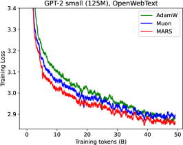
(a) Training Loss

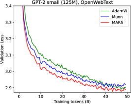
(b) Validation Loss

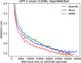
(c) Wall-clock time

Figure 1: The training and validation loss curves, plotted against both training tokens and wall-clock time on GPT-2 small model (125M).

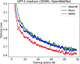
(a) Training Loss

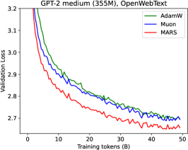
(b) Validation Loss

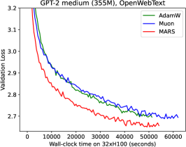
(c) Wall-clock time

Figure 2: The training and validation loss curves, plotted against both training tokens and wall-clock time on GPT-2 medium model (355M).

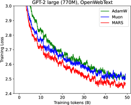
(a) Training Loss

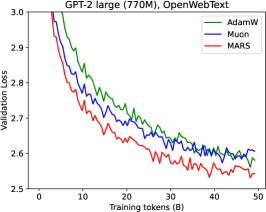
(b) Validation Loss

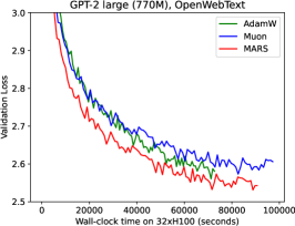
(c) Wall-clock time

Figure 3: The training and validation loss curves, plotted against both training tokens and wall-clock time on GPT-2 large model (770M).

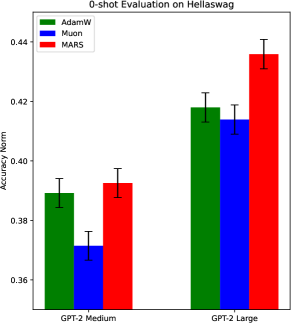
Figure 4: The accuracy for 0-shot evalution on Hellaswag (Zellers et al., 2019) dataset for AdamW, Muon and MARS on GPT-2 medium (355M) and large (770M) models.

4.2 Results

In Figures 1, 2, and 3, we demonstrate the training and validation losses as a function of training tokens and wall-clock time for various model sizes. Across the small, medium, and large GPT-2 models, MARS consistently surpasses both the AdamW and Muon baselines in training and validation losses. The performance gap becomes more pronounced with increasing model size. Notably, MARS exhibits both rapid initial decay and sustained superiority throughout the training process. Further, we explore the performance of additional learning rate choices in Appendix B. Notably, the best validation loss of MARS achieved in our GPT-2 small experiments is 2.852. For comparison, Sophia-H (Liu et al., 2023) achieves a validation loss of 2.901, and Sophia-G (Liu et al., 2023) achieves 2.875 under the same settings and datasets as ours. These results demonstrate that our reported performance is highly competitive with state-of-the-art optimizers.

In Figure 1(c), 2(c), and 3(c), we compare the wall-clock time of different algorithms. We observe that our algorithm, MARS, has a slightly higher per-iteration cost compared to AdamW but is much faster than Muon. Additionally, MARS consistently demonstrates lower validation losses than both AdamW and Muon within equivalent training durations.

We also test our optimization algorithm on the downstream task of commonsense natural language inference using the Hellaswag dataset (Zellers et al., 2019), evaluated with $0$-shot. The results, shown in Figure 4, are obtained from GPT-2 medium and large models pre-trained for 100,000 steps (50B tokens). The models pre-trained with MARS outperformed those pre-trained with AdamW and Muon optimizers, validating an enhanced downstream performance within the same number of pre-training steps.

4.3 MARS and MARS-approx.

We then conduct experiments to compare the performance of MARS and MARS-approx (MARS-AdamW version) on GPT-2 small and medium models, the results are shown in Figure 5. Models trained with MARS exhibit slightly better performance than those trained with MARS-approx, though the performance gap in terms of training tokens is marginal. This suggests that the approximate version is a practical alternative in scenarios where computational cost is a priority, as it introduces only minimal performance loss. However, in settings where achieving higher validation accuracy is critical, the exact version is recommended.

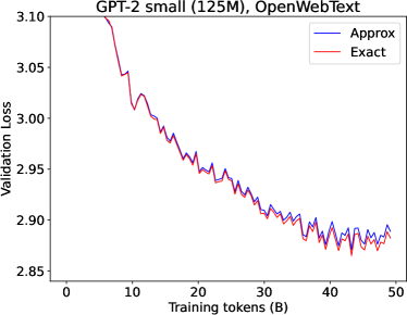
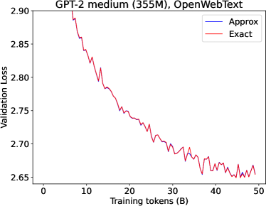
Figure 5: Validation loss curves for MARS and MARS-approx on GPT-2 small (125M, left) and medium (355M, right).

5 Related Work

In this section, we provide a review of additional related works, including some previously mentioned, to help readers gain a deeper understanding of the history and development of adaptive gradient methods and variance reduction techniques.

Adaptive Gradient Methods.

RProp (Riedmiller and Braun, 1993) is probably one of the earliest adaptive gradient methods by dynamically adjusting the learning rate. AdaGrad (Duchi et al., 2011; McMahan and Streeter, 2010) adjusts the learning rate based on the geometry of the training data observed during earlier iterations. To tackle with the issue of diminishing gradient in AdaGrad, Tieleman (2012) introduced RMSProp by incorporating the idea of exponential moving average. A significant advancement came with Adam (Kingma, 2014), which integrated RMSProp with Nesterov’s momentum (Nesterov, 1983, 2013) achieving superior performance and becoming a prevalent optimizer in deep neural network training. Later, Loshchilov (2017) proposed to decouple weight decay from gradient calculations in Adam and introduced AdamW, an optimization algorithm having become the predominant optimization algorithm in contemporary deep learning applications. To fix the convergence issue of Adam, Reddi et al. (2019) introduced the AMSGrad optimizer, which maintains a running maximum of past second-order momentum terms to achieve non-increasing step sizes. Subsequently, Chen et al. (2018) unified AMSGrad and SGD within the Padam framework by introducing a partial adaptive parameter to control the degree of adaptiveness. Notably, AdamW and its variations have been widely used in the training of popular large language models, including OPT (Zhang et al., 2022), Llama 3 (Dubey et al., 2024), and DeepSeek-V2 (Liu et al., 2024).

Variance Reduction Methods.

SAG(Roux et al., 2012) and SDCA(Shalev-Shwartz and Zhang, 2013) were among the first attempts to apply variance reduction techniques to accelerate the convergence of SGD. Subsequently, simpler algorithms like SVRG(Johnson and Zhang, 2013) and SAGA(Defazio et al., 2014) were introduced, achieving the same improved convergence rates. SARAH (Nguyen et al., 2017a) further simplified these approaches by employing biased recursive gradient estimation, which reduces storage requirements while achieving the complexity bounds for convex optimization problems. For non-convex optimization, besides SVRG (Allen-Zhu and Yuan, 2016; Reddi et al., 2016) and SARAH (Nguyen et al., 2017b), SPIDER (Fang et al., 2018) integrates Normalized Gradient Descent (Nesterov, 2013; Hazan et al., 2015) with recursive estimation of gradients, while SNVRG (Zhou et al., 2020) introduces multiple reference points for semi-stochastic gradient calculation for improved variance reduction and convergence rate. SpiderBoost (Wang et al., 2019) refines SPIDER by enabling the use of a significantly larger constant step size while preserving the same near-optimal oracle complexity. Subsequently, STORM (Cutkosky and Orabona, 2019) was proposed to further simplifies the SPIDER and SNVRG algorithms through the use of stochastic recursive momentum. This was later improved into a parameter-free variant, namely STORM+(Levy et al., 2021).

Variance Reduction for Adaptive Gradient Methods.

Few works have explored the application of variance reduction techniques to adaptive gradient methods. To the best of our knowledge, the only exceptions are Adam⁺ and SuperAdam. Adam⁺ (Liu et al., 2020) attempts to reduce the variance of first-order moment in Adam by estimating the gradient only at extrapolated points. SuperAdam (Huang et al., 2021), an adaptive gradient algorithm that integrates variance reduction with AdamW to achieve improved convergence rates. However, these variance-reduced adaptive gradient methods have primarily been validated on basic computer vision tasks, such as MNIST (Schölkopf and Smola, 2002) and CIFAR-10 (Krizhevsky et al., 2009), and simple natural language modeling tasks, like SWB-300 (Saon et al., 2017), using straightforward architectures such as LeNet (LeCun et al., 1998), ResNet-32 (He et al., 2016), 2-layer LSTMs (Graves and Graves, 2012), and 2-layer Transformers (Vaswani, 2017). As a result, a significant gap remains in the successful application of variance reduction techniques to adaptive gradient methods, particularly in the rapidly evolving domain of large language models.

6 Conclusion

In this work, we introduce MARS, a unified framework for adaptive gradient methods that integrates variance reduction techniques to improve the training of large models. Our approach combines the adaptive learning rate introduced by preconditioning with the faster convergence enabled by variance reduction. Within our framework, we have developed three optimization algorithms based on the ideas of AdamW, Lion, and Shampoo. Through extensive empirical experiments on GPT-2 pre-training tasks, we demonstrate that MARS consistently outperforms baseline algorithms in terms of both token efficiency and wall-clock time. Our results establish a generic framework for combining adaptive gradient methods with variance reduction techniques, contributing to the advancement of optimizers in large model training.

Appendix A Proofs of Lemma 3.4

Proof of Lemma 3.4.

Substituting (3.23) into (3.24), we obtain

$$\mathbf{m}_{t}=b_{1}\big{(}a_{1}\mathbf{u}_{t-1}+a_{2}\mathbf{g}_{t}\big{)}+b_{2}\mathbf{g}_{t}=a_{1}b_{1}\mathbf{u}_{t-1}+(b_{1}a_{2}+b_{2})\mathbf{g}_{t}.$$ (A.1)

On the other hand, shifting the index of (3.24) by $1$, we have

$$\mathbf{m}_{t-1}=b_{1}\mathbf{u}_{t-1}+b_{2}\mathbf{g}_{t-1}.$$ (A.2)

Combining (A.1) and (A.2), we obtain the iterative update of $\mathbf{m}_{t}$ from its previous value $\mathbf{m}_{t-1}$ as:

$$\mathbf{m}_{t} =a_{1}\mathbf{m}_{t-1}-a_{1}b_{2}\mathbf{g}_{t-1}+(b_{1}a_{2}+b_{2})\mathbf{g}_{t}$$

$$=a_{1}\mathbf{m}_{t-1}+(b_{1}a_{2}-a_{1}b_{2}+b_{2})\mathbf{g}_{t}+a_{1}b_{2}(\mathbf{g}_{t}-\mathbf{g}_{t-1}).$$

This completes the proof. ∎

Appendix B Additional Experiments

B.1 Learning Rates

In our experiments, we explore various learning rate choices on GPT-2 small. AdamW with a learning rate of $6\times 10^{-4}$ demonstrates superior performance in terms of validation loss during the initial 37 billion tokens of training. However, a higher learning rate of $3\times 10^{-3}$ yields significantly better results in the final 13 billion tokens. We then further extend our experiments by comparing AdamW and MARS-AdamW under identical hyperparameters, both using the higher learning rate of $3\times 10^{-3}$. The results, presented in Figure 6, show that even against an alternative baseline with hyperparameters optimized for AdamW, MARS-AdamW consistently outperforms AdamW. We observe that there is still potential for further parameter tuning and performance improvements with MARS.

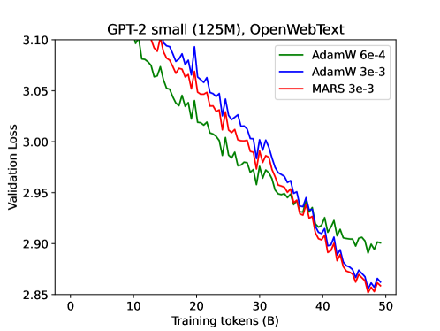
Figure 6: Validation loss with respect to training tokens for AdamW with learning rates $6\times 10^{-4}$, $3\times 10^{-3}$ and MARS with learning rate $3\times 10^{-3}$ on GPT-2 small model (125M). The model trained with MARS achieves a validation loss of 2.852.

B.2 Comparison between MARS and Lion

The key difference between MARS-AdamW and MARS-Lion lies in their precondition matrix. We evaluate MARS-AdamW against MARS-Lion under identical hyperparameters on GPT-2 small. As shown in Figure 7, MARS-AdamW outperforms MARS-Lion in both training and validation loss. Therefore, we mainly use MARS-AdamW in the rest of our experiments.

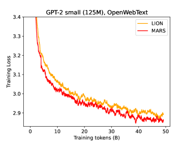
(a) Training Loss

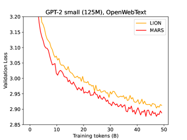
(b) Validation Loss

Figure 7: The training and validation loss curves, plotted against training tokens for Lion and MARS on GPT-2 small model (125M).

B.3 Sensitivity to $\gamma$.

To explore the impact of $\gamma_{t}$, we tested various $\gamma_{t}$ schedules, including constant and linearly changing schedules. Other hyper-parameters are set the same as the main experiments, and the results are summarized in Table 1. Specifically, the constant $\gamma$ values of 0.025 and 0.05 exhibit the best performance among the $\gamma_{t}$-schedules evaluated. We are using a $\gamma_{t}$ schedule of $0.025$ across all our other experiments.

Table 1: The validation loss for GPT-2 small (125M) model with different $\gamma$-schedules.

$\gamma$-schedule	$\gamma$	Validation loss
Constant	0.025	2.871
	0.05	2.871
Changing	0.025$\rightarrow$0.05	2.872
	0.1$\rightarrow$0	2.873
	0$\rightarrow$0.1	2.891
	0$\rightarrow$0.2	2.899

Appendix C Hyper-parameter Choices

Table 2 summarizes the architectural hyperparameters for GPT-2 models with 125M (small), 355M (medium), and 770M (large) parameters. Table 3 lists the general hyperparameters used across all experiments, while Tables 4, 5 and 6 present the training hyperparameters for the small, medium, and large models, respectively.

Table 2: Architecture hyperparameters for GPT-2 series models (Radford et al., 2019).

Model	#Param	#Layer	$n_{\text{head}}$	$d_{\text{emb}}$
GPT-2 small	125M	12	12	768
GPT-2 medium	355M	24	16	1024
GPT-2 large	770M	36	20	1280

Table 3: General hyper-parameters for the experiments.

Hyper-parameter	Value
Steps	100,000
Batch size in total	480
Context length	1024
Gradient clipping threshold	1.0
Dropout	0.0
Learning rate schedule	Cosine
Warm-up steps	2000
Base seed	5000

Table 4: Hyper-parameters for GPT-2 small experiment. We use $\gamma_{t}\equiv 0.025$ for MARS.

Hyper-parameter	AdamW	Muon	MARS
Max learning rate	6e-4	2e-2	6e-3
Min learning rate	3e-5	3e-5	3e-5
$(\beta_{1},\beta_{2})$	(0.9, 0.95)	$\mu=0.95$	(0.95, 0.99)

Table 5: Hyper-parameters for GPT-2 medium experiment. We use $\gamma_{t}\equiv 0.025$ for MARS.

Hyper-parameter	AdamW	Muon	MARS
Max learning rate	3e-4	1e-2	3e-3
Min learning rate	6e-5	6e-5	6e-5
$(\beta_{1},\beta_{2})$	(0.9, 0.95)	$\mu=0.95$	(0.95, 0.99)

Table 6: Hyper-parameters for GPT-2 large experiment. We use $\gamma_{t}\equiv 0.025$ for MARS.

Hyper-parameter	AdamW	Muon	MARS
Max learning rate	2e-4	6.67e-3	2e-3
Min learning rate	1e-5	1e-5	1e-5
$(\beta_{1},\beta_{2})$	(0.9, 0.95)	$\mu=0.95$	(0.95, 0.99)

References

- Allen-Zhu and Yuan (2016) Allen-Zhu, Z. and Yuan, Y. (2016). Improved svrg for non-strongly-convex or sum-of-non-convex objectives. In International conference on machine learning. PMLR.
- Anil et al. (2020) Anil, R., Gupta, V., Koren, T., Regan, K. and Singer, Y. (2020). Scalable second order optimization for deep learning. arXiv preprint arXiv:2002.09018 .
- Arjevani et al. (2023) Arjevani, Y., Carmon, Y., Duchi, J. C., Foster, D. J., Srebro, N. and Woodworth, B. (2023). Lower bounds for non-convex stochastic optimization. Mathematical Programming 199 165–214.
- Bernstein and Newhouse (2024) Bernstein, J. and Newhouse, L. (2024). Old optimizer, new norm: An anthology. arXiv preprint arXiv:2409.20325 .
- Brown (2020) Brown, T. B. (2020). Language models are few-shot learners. arXiv preprint arXiv:2005.14165 .
- Chen et al. (2018) Chen, J., Zhou, D., Tang, Y., Yang, Z., Cao, Y. and Gu, Q. (2018). Closing the generalization gap of adaptive gradient methods in training deep neural networks. arXiv preprint arXiv:1806.06763 .
- Chen et al. (2023) Chen, X., Liang, C., Huang, D., Real, E., Wang, K., Pham, H., Dong, X., Luong, T., Hsieh, C.-J., Lu, Y. et al. (2023). Symbolic discovery of optimization algorithms. Advances in neural information processing systems 36.
- Chowdhery et al. (2023) Chowdhery, A., Narang, S., Devlin, J., Bosma, M., Mishra, G., Roberts, A., Barham, P., Chung, H. W., Sutton, C., Gehrmann, S. et al. (2023). Palm: Scaling language modeling with pathways. Journal of Machine Learning Research 24 1–113.
- Cutkosky and Orabona (2019) Cutkosky, A. and Orabona, F. (2019). Momentum-based variance reduction in non-convex sgd. Advances in neural information processing systems 32.
- Defazio et al. (2014) Defazio, A., Bach, F. and Lacoste-Julien, S. (2014). Saga: A fast incremental gradient method with support for non-strongly convex composite objectives. Advances in neural information processing systems 27.
- Defazio and Bottou (2019) Defazio, A. and Bottou, L. (2019). On the ineffectiveness of variance reduced optimization for deep learning. Advances in Neural Information Processing Systems 32.
- Devlin (2018) Devlin, J. (2018). Bert: Pre-training of deep bidirectional transformers for language understanding. arXiv preprint arXiv:1810.04805 .
- Dubey et al. (2024) Dubey, A., Jauhri, A., Pandey, A., Kadian, A., Al-Dahle, A., Letman, A., Mathur, A., Schelten, A., Yang, A., Fan, A. et al. (2024). The llama 3 herd of models. arXiv preprint arXiv:2407.21783 .
- Duchi et al. (2011) Duchi, J., Hazan, E. and Singer, Y. (2011). Adaptive subgradient methods for online learning and stochastic optimization. Journal of machine learning research 12.
- Fang et al. (2018) Fang, C., Li, C. J., Lin, Z. and Zhang, T. (2018). Spider: Near-optimal non-convex optimization via stochastic path-integrated differential estimator. Advances in neural information processing systems 31.
- Ghadimi and Lan (2013) Ghadimi, S. and Lan, G. (2013). Stochastic first-and zeroth-order methods for nonconvex stochastic programming. SIAM journal on optimization 23 2341–2368.
- Gokaslan et al. (2019) Gokaslan, A., Cohen, V., Pavlick, E. and Tellex, S. (2019). Openwebtext corpus. http://Skylion007.github.io/OpenWebTextCorpus.
- Graves and Graves (2012) Graves, A. and Graves, A. (2012). Long short-term memory. Supervised sequence labelling with recurrent neural networks 37–45.
- Gupta et al. (2018) Gupta, V., Koren, T. and Singer, Y. (2018). Shampoo: Preconditioned stochastic tensor optimization. In International Conference on Machine Learning. PMLR.
- Hazan et al. (2015) Hazan, E., Levy, K. and Shalev-Shwartz, S. (2015). Beyond convexity: Stochastic quasi-convex optimization. Advances in neural information processing systems 28.
- He et al. (2016) He, K., Zhang, X., Ren, S. and Sun, J. (2016). Deep residual learning for image recognition. In Proceedings of the IEEE conference on computer vision and pattern recognition.
- Higham (2008) Higham, N. J. (2008). Functions of Matrices. Society for Industrial and Applied Mathematics.
- Huang et al. (2021) Huang, F., Li, J. and Huang, H. (2021). Super-adam: faster and universal framework of adaptive gradients. Advances in Neural Information Processing Systems 34 9074–9085.
- Johnson and Zhang (2013) Johnson, R. and Zhang, T. (2013). Accelerating stochastic gradient descent using predictive variance reduction. Advances in neural information processing systems 26.
- Jordan et al. (2024) Jordan, K. et al. (2024). KellerJordan/modded-nanogpt: NanoGPT (124M) quality in 8.2 minutes. https://github.com/KellerJordan/modded-nanogpt.
- Kaddour et al. (2024) Kaddour, J., Key, O., Nawrot, P., Minervini, P. and Kusner, M. J. (2024). No train no gain: Revisiting efficient training algorithms for transformer-based language models. Advances in Neural Information Processing Systems 36.
- Karpathy (2022) Karpathy, A. (2022). NanoGPT. https://github.com/karpathy/nanoGPT.
- Kingma (2014) Kingma, D. P. (2014). Adam: A method for stochastic optimization. arXiv preprint arXiv:1412.6980 .
- Krizhevsky et al. (2009) Krizhevsky, A., Hinton, G. et al. (2009). Learning multiple layers of features from tiny images .
- Lakić (1998) Lakić, S. (1998). On the computation of the matrix k-th root. ZAMM-Journal of Applied Mathematics and Mechanics/Zeitschrift für Angewandte Mathematik und Mechanik: Applied Mathematics and Mechanics 78 167–172.
- LeCun et al. (1998) LeCun, Y., Bottou, L., Bengio, Y. and Haffner, P. (1998). Gradient-based learning applied to document recognition. Proceedings of the IEEE 86 2278–2324.
- Levy et al. (2021) Levy, K., Kavis, A. and Cevher, V. (2021). Storm+: Fully adaptive sgd with recursive momentum for nonconvex optimization. Advances in Neural Information Processing Systems 34 20571–20582.
- Liu et al. (2024) Liu, A., Feng, B., Wang, B., Wang, B., Liu, B., Zhao, C., Dengr, C., Ruan, C., Dai, D., Guo, D. et al. (2024). Deepseek-v2: A strong, economical, and efficient mixture-of-experts language model. arXiv preprint arXiv:2405.04434 .
- Liu et al. (2023) Liu, H., Li, Z., Hall, D., Liang, P. and Ma, T. (2023). Sophia: A scalable stochastic second-order optimizer for language model pre-training. arXiv preprint arXiv:2305.14342 .
- Liu et al. (2020) Liu, M., Zhang, W., Orabona, F. and Yang, T. (2020). Adam +: A stochastic method with adaptive variance reduction. arXiv preprint arXiv:2011.11985 .
- Loshchilov (2017) Loshchilov, I. (2017). Decoupled weight decay regularization. arXiv preprint arXiv:1711.05101 .
- Martens and Grosse (2015) Martens, J. and Grosse, R. (2015). Optimizing neural networks with kronecker-factored approximate curvature. In International conference on machine learning. PMLR.
- Martinsson and Tropp (2020) Martinsson, P.-G. and Tropp, J. A. (2020). Randomized numerical linear algebra: Foundations and algorithms. Acta Numerica 29 403–572.
- McCandlish et al. (2018) McCandlish, S., Kaplan, J., Amodei, D. and Team, O. D. (2018). An empirical model of large-batch training. arXiv preprint arXiv:1812.06162 .
- McMahan and Streeter (2010) McMahan, H. B. and Streeter, M. (2010). Adaptive bound optimization for online convex optimization. arXiv preprint arXiv:1002.4908 .
- Morwani et al. (2024) Morwani, D., Shapira, I., Vyas, N., Malach, E., Kakade, S. and Janson, L. (2024). A new perspective on shampoo’s preconditioner. arXiv preprint arXiv:2406.17748 .
- Nesterov (1983) Nesterov, Y. (1983). A method for solving the convex programming problem with convergence rate . Proceedings of the USSR Academy of Sciences 269 543–547.
- Nesterov (2013) Nesterov, Y. (2013). Introductory lectures on convex optimization: A basic course, vol. 87. Springer Science & Business Media.
- Nguyen et al. (2017a) Nguyen, L. M., Liu, J., Scheinberg, K. and Takáč, M. (2017a). Sarah: A novel method for machine learning problems using stochastic recursive gradient. In International conference on machine learning. PMLR.
- Nguyen et al. (2017b) Nguyen, L. M., Liu, J., Scheinberg, K. and Takáč, M. (2017b). Stochastic recursive gradient algorithm for nonconvex optimization. arXiv preprint arXiv:1705.07261 .
- Radford et al. (2019) Radford, A., Wu, J., Child, R., Luan, D., Amodei, D., Sutskever, I. et al. (2019). Language models are unsupervised multitask learners. OpenAI blog 1 9.
- Reddi et al. (2016) Reddi, S. J., Hefny, A., Sra, S., Poczos, B. and Smola, A. (2016). Stochastic variance reduction for nonconvex optimization. In International conference on machine learning. PMLR.
- Reddi et al. (2019) Reddi, S. J., Kale, S. and Kumar, S. (2019). On the convergence of adam and beyond. arXiv preprint arXiv:1904.09237 .
- Riedmiller and Braun (1993) Riedmiller, M. and Braun, H. (1993). A direct adaptive method for faster backpropagation learning: The rprop algorithm. In IEEE international conference on neural networks. IEEE.
- Roux et al. (2012) Roux, N., Schmidt, M. and Bach, F. (2012). A stochastic gradient method with an exponential convergence _rate for finite training sets. Advances in neural information processing systems 25.
- Saon et al. (2017) Saon, G., Kurata, G., Sercu, T., Audhkhasi, K., Thomas, S., Dimitriadis, D., Cui, X., Ramabhadran, B., Picheny, M., Lim, L.-L. et al. (2017). English conversational telephone speech recognition by humans and machines. arXiv preprint arXiv:1703.02136 .
- Schölkopf and Smola (2002) Schölkopf, B. and Smola, A. J. (2002). Learning with kernels: support vector machines, regularization, optimization, and beyond. MIT press.
- Schulz (1933) Schulz, G. (1933). Iterative berechnung der reziproken matrix. Z. Angew. Math. Mech. 13 57–59.
- Shalev-Shwartz and Zhang (2013) Shalev-Shwartz, S. and Zhang, T. (2013). Stochastic dual coordinate ascent methods for regularized loss minimization. Journal of Machine Learning Research 14.
- Shazeer and Stern (2018) Shazeer, N. and Stern, M. (2018). Adafactor: Adaptive learning rates with sublinear memory cost. In International Conference on Machine Learning. PMLR.
- Srivastava et al. (2014) Srivastava, N., Hinton, G., Krizhevsky, A., Sutskever, I. and Salakhutdinov, R. (2014). Dropout: a simple way to prevent neural networks from overfitting. The journal of machine learning research 15 1929–1958.
- Tieleman (2012) Tieleman, T. (2012). Lecture 6.5-rmsprop: Divide the gradient by a running average of its recent magnitude. COURSERA: Neural networks for machine learning 4 26.
- Vaswani (2017) Vaswani, A. (2017). Attention is all you need. Advances in Neural Information Processing Systems .
- Vyas et al. (2024) Vyas, N., Morwani, D., Zhao, R., Shapira, I., Brandfonbrener, D., Janson, L. and Kakade, S. (2024). Soap: Improving and stabilizing shampoo using adam. arXiv preprint arXiv:2409.11321 .
- Wang et al. (2019) Wang, Z., Ji, K., Zhou, Y., Liang, Y. and Tarokh, V. (2019). Spiderboost and momentum: Faster variance reduction algorithms. Advances in Neural Information Processing Systems 32.
- Ward et al. (2020) Ward, R., Wu, X. and Bottou, L. (2020). Adagrad stepsizes: Sharp convergence over nonconvex landscapes. Journal of Machine Learning Research 21 1–30.
- Xie et al. (2024) Xie, X., Zhou, P., Li, H., Lin, Z. and Yan, S. (2024). Adan: Adaptive nesterov momentum algorithm for faster optimizing deep models. IEEE Transactions on Pattern Analysis and Machine Intelligence .
- You et al. (2019) You, Y., Li, J., Reddi, S., Hseu, J., Kumar, S., Bhojanapalli, S., Song, X., Demmel, J., Keutzer, K. and Hsieh, C.-J. (2019). Large batch optimization for deep learning: Training bert in 76 minutes. arXiv preprint arXiv:1904.00962 .
- Zeiler (2012) Zeiler, M. D. (2012). Adadelta: an adaptive learning rate method. arXiv preprint arXiv:1212.5701 .
- Zellers et al. (2019) Zellers, R., Holtzman, A., Bisk, Y., Farhadi, A. and Choi, Y. (2019). Hellaswag: Can a machine really finish your sentence? arXiv preprint arXiv:1905.07830 .
- Zhang et al. (2022) Zhang, S., Roller, S., Goyal, N., Artetxe, M., Chen, M., Chen, S., Dewan, C., Diab, M., Li, X., Lin, X. V. et al. (2022). Opt: Open pre-trained transformer language models. arXiv preprint arXiv:2205.01068 .
- Zhao et al. (2024) Zhao, R., Morwani, D., Brandfonbrener, D., Vyas, N. and Kakade, S. (2024). Deconstructing what makes a good optimizer for language models. arXiv preprint arXiv:2407.07972 .
- Zhou et al. (2020) Zhou, D., Xu, P. and Gu, Q. (2020). Stochastic nested variance reduction for nonconvex optimization. Journal of machine learning research 21 1–63.
- Zhuang et al. (2020) Zhuang, J., Tang, T., Ding, Y., Tatikonda, S. C., Dvornek, N., Papademetris, X. and Duncan, J. (2020). Adabelief optimizer: Adapting stepsizes by the belief in observed gradients. Advances in neural information processing systems 33 18795–18806.