Dynamic Causal Effects in a Nonlinear World:
the Good, the Bad, and the Ugly

Abstract:

Applied macroeconomists frequently use impulse response estimators motivated by linear models. We study whether the estimands of such procedures have a causal interpretation when the true data generating process is in fact nonlinear. We show that vector autoregressions and linear local projections onto observed shocks or proxies identify weighted averages of causal effects regardless of the extent of nonlinearities. By contrast, identification approaches that exploit heteroskedasticity or non-Gaussianity of latent shocks are highly sensitive to departures from linearity. Our analysis is based on new results on the identification of marginal treatment effects through weighted regressions, which may also be of interest to researchers outside macroeconomics.

Keywords: dynamic treatment effect, impulse response, local projection, semiparametric identification, structural vector autoregression.

1 Introduction

Impulse response functions are key objects in macroeconomic analysis. Since they measure dynamic causal effects of surprise changes in policy or fundamentals on subsequent macroeconomic outcomes, they provide calibration targets for structural modeling and help validate model predictions. They also inform optimal economic policy questions, both directly and indirectly (Christiano, Eichenbaum, and Evans, 1999; McKay and Wolf, 2023).

Applied researchers typically report impulse response estimators motivated by linear time series models, such as vector autoregressions or local projections. Although there exists a wealth of nonlinear alternatives (Fan and Yao, 2003; Herbst and Schorfheide, 2016; Kilian and Lütkepohl, 2017, Chapter 18), linear methods are attractive due to their simplicity and the difficulty of clearly detecting nonlinear relationships in typical macroeconomic data. At the same time, both macroeconomic theorists and policymakers think nonlinearities are important: structural models with essential nonlinearities have become dominant in recent decades, and many economic policy debates concern state-dependence and asymmetries. How can we justify using linear methods if we think the world is a nonlinear place?

This paper studies the causal interpretation of impulse response estimators based on linear models when the data is generated by an essentially unrestricted nonparametric structural model. We first deliver good news for linear local projection or VAR estimators that project directly on an observed shock or proxy: their estimand (i.e., probability limit) equals a weighted average of the true nonlinear causal effects, regardless of the extent of nonlinearities in the data generating process (DGP). By contrast, the news is bad or even ugly for estimators that identify latent shocks via heteroskedasticity or non-Gaussianity: they generally do not estimate a meaningful causal summary under departures from linearity. Thus, the hard work needed to directly measure shocks (or proxies) using historical or institutional data buys insurance against nonlinearities that other identification approaches lack.

Our good news are based on an extension of the results in Yitzhaki (1996) and Rambachan and Shephard (2021): impulse response estimands from linear local projections and VARs that project on observed shocks or proxies correspond to positively-weighted averages of marginal effects—effects of infinitesimally small shocks that average out over all (past, present, and future) shocks other than the contemporaneous shock of interest, weighted over different baseline shock values. Thus, these estimands provide a scalar causal summary of the full richness of the nonlinear causal effects; the positive weights ensure that the researcher gets the sign right if the true marginal effects are uniformly positive or negative. Our assumptions drop restrictions imposed in the existing literature that ruled out models with kinks or discontinuous regime-switches or shocks with unbounded support.

In a nonlinear DGP, both the sign and the magnitude of the causal effects can depend on the baseline shock value (e.g., whether it is positive or negative), so how these values are weighted can matter a lot. Fortunately, as we illustrate using several empirical examples, the weight function used by local projections and VARs is straightforward to estimate and report. In many applications the researcher does not directly observe the shock of interest but only a proxy, also known as an external instrument (Stock and Watson, 2018). In this case, we show that an easily-interpretable monotonicity condition is required to guarantee a positive weight function. We also show that directly modeling the nonlinearities can be counterproductive unless the researcher is confident in their modeling: under functional form misspecification, local projections with higher-order terms still estimate a weighted average of marginal effects, but some of the weights may be negative, which risks getting the sign of the causal effects wrong. Finally, we discuss how the results change when control variables are needed to isolate a true shock (i.e., recursive or Cholesky identification).

When there is a dearth of direct shock measures or proxies, applied researchers frequently resort to identification via heteroskedasticity (Sentana and Fiorentini, 2001; Rigobon, 2003; Lewbel, 2012). Unfortunately, we show that these estimation approaches are sensitive to the assumption that the structural model is linear: the estimand can easily be nonzero when there is no causal effect, or negative when the true shock has a uniformly positive effect on the outcome of interest. Fixing these issues while still delivering informative inference appears difficult, since a natural nonparametric generalization of the identification strategy yields very wide identified sets. The intuition for these negative results is that the identification exploits a source of exogenous variation that shifts the scale of the latent shock of interest but not its mean. Without strong functional form assumptions, this type of exogenous variation is uninformative about the effect of a location shift in the shock on the conditional mean of the outcome, i.e., the impulse response. However, a silver lining is that the linear model delivers testable restrictions.

The sensitivity to nonlinearity is even greater for identification via non-Gaussianity (Comon, 1994; Gouriéroux, Monfort, and Renne, 2017; Lanne, Meitz, and Saikkonen, 2017). Also known as independent components analysis (ICA), this identification approach has recently increased significantly in popularity in the VAR literature. We show that the nonparametric analogue of the identification assumptions yields an identified set so large that effectively any function of the data can be construed as a “shock”. Intuitively, the mere assumptions that the latent shocks are independent and non-Gaussian are vacuous in a nonparametric context: any collection of random variables can always be represented as some nonlinear function of independent uniformly distributed random variables. Moreover, we give examples of simple DGPs featuring slight nonlinearity for which any linearity-based ICA procedure is highly biased asymptotically, yet in these DGPs one cannot reject the validity of the linear model.

The building block underlying most of the above findings is a set of results on the identification of weighted averages of marginal treatment effects using weighted regressions, which connects our analysis to a large literature in microeconometrics (e.g., Yitzhaki, 1996; Newey and Stoker, 1993; Angrist and Krueger, 1999; Goldsmith-Pinkham, Hull, and Kolesár, 2024). We extend existing results in this literature by unifying the treatment of continuous, discrete, and mixed regressors, and by substantially weakening the regularity conditions: we allow for regressors with unbounded support, impose minimal regularity on the regression function, and our moment conditions essentially only require the existence of the probability limit of the regression estimator.

An important limitation of our results is that they only concern identification. While we are motivated by the observation that full-fledged nonparametric estimation is challenging in realistic macroeconomic data sets, we do not explicitly analyze the precision or small-sample bias of the estimators we study. We refer to Herbst and Johannsen (2024) for a discussion of finite-sample biases of local projections and VARs in linear models.

Literature.

Pioneering work on semiparametric causal time series analysis includes Gallant, Rossi, and Tauchen (1993), White (2006), White and Kennedy (2009), Angrist and Kuersteiner (2011), and Angrist, Jordà, and Kuersteiner (2018), see also Gonçalves, Herrera, Kilian, and Pesavento (2021, 2024), Gouriéroux and Lee (2023), and Kitagawa, Wang, and Xu (2023) for recent contributions. Our result on the causal interpretation of local projections with observed shocks is very closely related to Rambachan and Shephard (2021) and subsequent work by Caravello and Martínez Bruera (2024) and Casini and McCloskey (2024), but we impose substantively weaker assumptions, and also study the properties of the weight function.

As for identification via heteroskedasticity or non-Gaussianity, we are not aware of other work in a nonparametric vein. Montiel Olea, Plagborg-Møller, and Qian (2022) criticize linearity-based versions of these identification strategies for being seemingly sensitive to functional form assumptions, and potentially being subject to weak identification. The present analysis quantifies this sensitivity more precisely by deriving both the identified sets for the nonparametric analogues of these identification assumptions, and the estimands of linearity-based procedures.

Outline.

Section 2 defines a nonparametric framework for identification of dynamic causal effects. Section 3 argues that local projection and VAR estimands based on observed shocks or proxies have a robust causal interpretation regardless of the extent of nonlinearities. Sections 4 and 5 show, on the other hand, that estimands based on identification through heteroskedasticity or non-Gaussianity are sensitive to the assumption that the structural function is linear. Section 6 provides the theoretical basis for the results in the earlier parts of the paper by extending results from the microeconometric literature on the interpretation of regression estimators as weighted marginal treatment effects; this section may be of independent interest for readers outside macroeconomics. Section 7 concludes. Technical details and proofs are relegated to the appendix.

2 Nonparametric framework for dynamic causality

In this section we set up a nonparametric framework for dynamic causal identification.

2.1 Model

We are interested in the dynamic response of a scalar outcome variable $Y_{t}$ to an impulse in the scalar shock variable $X_{t}$. As a leading example, one may think of $X_{t}$ as a variable controlled by a policy-maker, such as a surprise change in the policy interest rate set by the central bank. For ease of exposition, we restrict attention to continuously distributed shocks $X_{t}$ for now, but Section 6 shows that our results generalize to handle continuous, discrete, or mixed distributions in a unified manner.

The outcome variable is determined by an underlying dynamic structural model. Our causal framework doesn’t restrict this model; we only assume that when evaluated $h$ periods after the realization of the shock $X_{t}$, the outcome admits the nonparametric structural representation

$$Y_{t+h}=\psi_{h}(X_{t},\bm{\mathbf{U}}_{h,t+h})\quad\text{for all }t,h\geq 0.$$ (1)

For each horizon $h$, $\psi_{h}(\cdot,\cdot)$ is an unknown measurable function that we call the structural function, while $\bm{\mathbf{U}}_{h,t+h}$ is a vector of all variables (dated before, on, and after time $t$) that causally affect $Y_{t+h}$, other than $X_{t}$. Without restrictions on $\bm{\mathbf{U}}_{h,t+h}$ or the structural function, the representation (1) is without loss of generality. In typical recursive time-series models, however, $\bm{\mathbf{U}}_{h,t+h}$ will contain the vector $\bm{\mathbf{Y}}_{t-1}$ of observed data at time $t-1$ as well as shocks dated $t,t+1,\dotsc,t+h$, but exclude $X_{t}$ or shocks dated after $t+h$ (White, 2006; White and Kennedy, 2009; Caravello and Martínez Bruera, 2024; Gonçalves, Herrera, Kilian, and Pesavento, 2024). A leading special case is the linear structural VAR model, which additionally implies that $\psi_{h}$ is linear in both $X_{t}$ and $\bm{\mathbf{U}}_{h,t+h}$ (e.g., Kilian and Lütkepohl, 2017, Chapter 4.1).

As is conventional in the literature, we assume that the shock of interest is independent of the nuisance shocks:

$$X_{t}\mathchoice{\mathrel{\hbox to0.0pt{$\displaystyle\perp$\hss}\mkern 2.0mu{\displaystyle\perp}}}{\mathrel{\hbox to0.0pt{$\textstyle\perp$\hss}\mkern 2.0mu{\textstyle\perp}}}{\mathrel{\hbox to0.0pt{$\scriptstyle\perp$\hss}\mkern 2.0mu{\scriptstyle\perp}}}{\mathrel{\hbox to0.0pt{$\scriptscriptstyle\perp$\hss}\mkern 2.0mu{\scriptscriptstyle\perp}}}\bm{\mathbf{U}}_{h,t+h}.$$ (2)

Given the interpretation of $X_{t}$ as a “shock”, this independence assumption essentially just normalizes the structural function $\psi_{h}$, so that its first argument captures the total causal effect of the shock $X_{t}$ on $Y_{t+h}$, including its direct effect and any indirect effects, both contemporaneous and dynamic. This is illustrated in the following simple example.

Example 1.

Consider a univariate AR(1) model with endogenous regime switching:

$$Y_{t}=\rho_{t}Y_{t-1}+\tau\varepsilon_{t}+\nu_{t},$$

with regime-dependent parameter $\rho_{t}=\rho_{1}S_{t}+\rho_{0}(1-S_{t})$ and binary regime $S_{t}=\operatorname{\mathbbm{1}}\{\varepsilon_{t-1}+\xi_{t-1}\leq 0\}$, and where $\rho_{0},\rho_{1},\tau$ are constants. Assume that $\varepsilon_{t}$, $\nu_{t}$, and $\xi_{t}$ are i.i.d. and mutually independent, and that we observe the shock $X_{t}=\varepsilon_{t}$. We can cast this model into the form required by equations 1 and 2 as follows. Define $\bm{\mathbf{U}}_{h,t+h}\equiv(Y_{t-1},S_{t},\nu_{t},\dotsc,\nu_{t+h},\xi_{t},\dotsc,\allowbreak\xi_{t+h-1},\varepsilon_{t+1},\dots,\varepsilon_{t+h})^{\prime}$ and $\rho(\vartheta)\equiv\rho_{1}\operatorname{\mathbbm{1}}\{\vartheta\leq 0\}+\rho_{0}\operatorname{\mathbbm{1}}\{\vartheta>0\}$ for $\vartheta\in\mathbb{R}$. Then, for all $h\geq 1$,

$$\psi_{h}(x,\bm{\mathbf{u}}) =\big{\{}y_{-1}(\rho_{1}s+\rho_{0}(1-s))+(\tau x+\nu)\big{\}}\rho(x+\xi)\prod_{\ell=1}^{h-1}\rho(\varepsilon_{+\ell}+\xi_{+\ell})$$

$$\quad+\sum_{\ell=1}^{h}(\tau\varepsilon_{+\ell}+\nu_{+\ell})\prod_{b=\ell}^{h-1}\rho(\varepsilon_{+b}+\xi_{+b}),$$

where we have partitioned $\bm{\mathbf{u}}=(y_{-1},s,\nu,\nu_{+1},\dots,\nu_{+h},\xi,\xi_{+1},\dots,\xi_{+(h-1)},\varepsilon_{+1},\dots,\varepsilon_{+h})^{\prime}$. Notice that the function $\psi_{h}$ captures the full dynamic effect of the shock variable $X_{t}=\varepsilon_{t}$: both the direct impact effect of $\varepsilon_{t}$ on $Y_{t}$ (which feeds forward to future periods), and the indirect, nonlinear effect of $\varepsilon_{t}$ on the next-period regime $S_{t+1}$ (which also feeds forward).

In some applications, such as when $X_{t}$ corresponds to a policy instrument rather than a surprise change in the instrument, one may wish to weaken the full independence assumption (2) to a conditional independence assumption—we discuss this extension in Section 3.3. Either way, it is meaningful to think of varying $X_{t}$ while keeping $\bm{\mathbf{U}}_{h,t+h}$ constant, so that the random function $x\mapsto\psi_{h}(x,\bm{\mathbf{U}}_{h,t+h})$ defines a potential outcome function at horizon $h$. One could work directly with these potential outcomes as in Angrist and Kuersteiner (2011), Angrist, Jordà, and Kuersteiner (2018), and Rambachan and Shephard (2021), and keep all other past, present, and future shocks (captured by $\bm{\mathbf{U}}_{h,t+h}$ in our model) implicit. Our structural function framework is mathematically equivalent, but facilitates comparisons with the linear structural VAR literature.

2.2 Causal effects

A familiar issue in nonlinear models is that there are multiple possible definitions of an impulse response, i.e., a dynamic causal effect. In a linear model, the effect of exogenously changing $X_{t}$ from $x_{0}$ to $x_{1}$ is a linear function of the difference $x_{1}-x_{0}$: it equals $\psi_{h}(x_{1},\bm{\mathbf{U}}_{h,t+h})-\psi_{h}(x_{0},\bm{\mathbf{U}}_{h,t+h})=\beta_{h}(x_{1}-x_{0})$ for some constant scalar $\beta_{h}$. By contrast, in a nonlinear model, the effect is a nonlinear function of the difference $x_{1}-x_{0}$, and it also generally depends on (i) the past history and the current and future nuisance shocks via $\bm{\mathbf{U}}_{h,t+h}$, as well as (ii) the sign and magnitude of $x_{0}$.

In theoretical macroeconomic modeling, researchers often report the impulse responses with respect to a so-called “MIT shock”, which starts the economy at steady state, then hits the economy with a one-off impulse to $X_{t}$, and subsequently sets all other current and future shocks to zero: $\psi_{h}(X_{t},\bm{\mathbf{0}})-\psi_{h}(0,\bm{\mathbf{0}})$, where we normalize the steady-state values of $X_{t}$ and $\bm{\mathbf{U}}_{h,t+h}$ to zero. While computationally convenient, this impulse response concept has no empirical counterpart and is not directly policy relevant in models that do not satisfy certainty equivalence.

We shall instead focus on impulse responses (causal effects) defined as expected counterfactual changes in the outcome of interest, averaging out over all other shocks. Specifically, define the average structural function

$$\Psi_{h}(x)\equiv E[\psi_{h}(x,\bm{\mathbf{U}}_{h,t+h})],\quad x\in\mathbb{R},$$

which corresponds to the expected potential outcome function. Here the expectation is taken over the marginal distribution of $\bm{\mathbf{U}}_{h,t+h}$. The expectation is implicitly assumed to exist for all $x$. The average structural function measures the counterfactual average value of the future outcome $Y_{t+h}$ that we would observe if the policy-maker engineered a particular fixed value $x$ for the policy variable at time $t$, averaging out over the randomness caused by all other factors that influence the outcome independently of the policy decision at time $t$. Even though in some nonlinear models the structural function $\psi_{h}$ is discontinuous in the policy variable $x$, the average structural function $\Psi_{h}$ will typically be a smoother function of $x$, as it averages out over the realizations of other shocks. For example, this is the case in the regime-switching model in 1 if $\xi_{t}$ is continuously distributed. A certain amount of smoothness in $\Psi_{h}$ will be important for the identification of causal effects, as we discuss below.

Typical data samples in macroeconomics are too small to permit accurate nonparametric estimation of the entire average structural function $x\mapsto\Psi_{h}(x)$. A pragmatic alternative is to target weighted averages of the structural function—average causal effects—or its derivatives—average marginal effects (Rambachan and Shephard, 2021; Gonçalves, Herrera, Kilian, and Pesavento, 2021, 2024). This paper focuses on estimation of average marginal effects

$$\theta_{h}(\omega)\equiv\int\omega(x)\Psi_{h}^{\prime}(x)\,dx,$$ (3)

where $\omega(\cdot)$ is a weight function averaging across the baseline values of the shock variable $X_{t}$. We reserve the term average marginal effect to weight functions that are convex, i.e., $\omega(x)$ is nonnegative for all $x$ and integrates to one, $\int\omega(x)\,dx=1$. This ensures that $\theta_{h}(\omega)$ is a meaningful causal summary of the average structural function $\Psi_{h}(x)$ in that it prevents what Small, Tan, Ramsahai, Lorch, and Brookhart (2017) call a sign-reversal: if $\Psi_{h}^{\prime}(x)$ has the same sign for all $x$ ($+,0$ or $-$), then $\theta_{h}(x)$ will also have this sign. This property is particularly useful when qualitatively validating predictions of structural macroeconomic models.

Depending on the form of the weight function, $\theta_{h}(\omega)$ has two interpretations in terms of an average causal effect of a shock with magnitude $\delta>0$,

$$\theta_{h}(\delta,\omega_{0})\equiv\frac{1}{\delta}\int\omega_{0}(x)\{\Psi_{h}(x+\delta)-\Psi_{h}(x)\}\,dx.$$ (4)

First, the average marginal effect corresponds to the average causal effect for infinitesimally small shocks: $\theta_{h}(\omega)=\lim_{\delta\to 0}\theta_{h}(\delta,\omega)$, provided we can pass the limit as $\delta\to 0$ under the integral sign in (4). Second, if the weighting in (3) admits the integral representation $\omega(x)=\frac{1}{\delta}\int_{x-\delta}^{x}\omega_{0}(x)\,dx$, substituting $\Psi_{h}(x+\delta)-\Psi_{h}(x)=\int_{x}^{x+\delta}\Psi^{\prime}(\chi)\,d\chi$ into (4) and changing the order of integration yields $\theta_{h}(\omega)=\theta_{h}(\delta,\omega_{0})$. For this reason, focusing on average marginal effects is without loss of generality.

In a linear model, the weighting does not matter, since $\Psi_{h}^{\prime}(x)$ does not depend on $x$. But in nonlinear models, it could matter greatly whether we attach most weight to positive or negative shocks, or to shocks with small or large magnitude. Therefore, accounting for the form of the weighting $\omega$ is important when using estimates of $\theta_{h}(\omega)$ to calibrate or validate structural macroeconomic models. In the next section, we discuss identification approaches that deliver weighted averages of marginal effects under a particular weighting scheme that depends on the shock distribution. In Section 6, we discuss estimation approaches that target any pre-specified weighting scheme.

3 The good: observed shocks and proxies

If the researcher directly observes the shock of interest, or at least a valid proxy for it, then there is good news: conventional local projections or structural VAR impulse responses estimate average marginal effects with an interpretable weighting scheme, regardless of how nonlinear the underlying DGP is. Moreover, the weights can be estimated from the data, and we give several empirical examples of how to interpret them. In contrast to linear estimators, we demonstrate using a simple example that nonlinear extensions of local projections or VARs do not generally provide meaningful causal summaries under misspecification. Finally, we extend the analysis to shocks that are recursively identified, i.e., by controlling for covariates.

3.1 Identification with observed shocks

We start off by assuming that the researcher directly observes (or consistently estimates) the shock $X_{t}$ of interest. This would be the case, for example, if the shock is identified through a “narrative approach”. See Ramey (2016) for several empirical examples.

Under the nonlinear structural model (1) and the shock independence assumption (2), the conditional expectation of the outcome given the shock,

$$g_{h}(x)\equiv E[Y_{t+h}\mid X_{t}=x],$$ (5)

nonparametrically identifies the average structural function:

$$\Psi_{h}(x)=E[\psi_{h}(x,\bm{\mathbf{U}}_{h,t+h})]=E[\psi_{h}(x,\bm{\mathbf{U}}_{h,t+h})\mid X_{t}=x]=g_{h}(x).$$ (6)

Hence, in principle, we could estimate any weighted causal effect of interest by running a nonparametric regression of $Y_{t+h}$ on $X_{t}$ to obtain $g_{h}(\cdot)$ in the first step, and then averaging this function according to the desired weighting scheme in the second step, as suggested by Gouriéroux and Lee (2023) and Gonçalves, Herrera, Kilian, and Pesavento (2024, Section 6). In Section 6, we discuss a complementary strategy that identifies the same estimand via weighted averages of the observed outcomes, and how both strategies can be combined. However, as discussed in more detail in Section 6, these strategies may yield noisy and sensitive estimates in the relatively small samples available in macroeconomics.

Interpretation of linear projection estimates.

We take a cue from Rambachan and Shephard (2021) and instead aim for a less ambitious goal. Rather than targeting a pre-specified weighted average of causal or marginal effects, we focus on simple local projection and VAR estimators, which are relatively precise even with small sample sizes. We demonstrate that these simple estimators have an attractive robustness property: even though they are motivated by a linear model, when the DGP is nonlinear, their estimand can still be interpreted as an average marginal effect with a particular weight function.

The local projection estimator of Jordà (2005) estimates the impulse response of $Y_{t}$ with respect to $X_{t}$ at horizon $h$ as the coefficient $\hat{\beta}_{h}$ in the ordinary least squares (OLS) regression

$$Y_{t+h}=\hat{\beta}_{h}X_{t}+\hat{\gamma}_{h}^{\prime}\bm{\mathbf{W}}_{t}+\text{residual}_{h,t+h},$$ (7)

where $\bm{\mathbf{W}}_{t}$ is a vector of control variables (typically including a constant and lagged outcomes and shocks). For now, we will assume that the shock $X_{t}$ is in fact a “shock”, so that it is linearly unpredictable using the controls: $\operatorname*{Cov}(X_{t},\bm{\mathbf{W}}_{t})=0$. Then the set of controls $\bm{\mathbf{W}}_{t}$ affects only the precision of $\hat{\beta}_{h}$, but not its probability limit. In particular, under standard stationarity and ergodicity assumptions, the local projection estimator $\hat{\beta}_{h}$ will converge in probability to the population projection coefficient

$$\beta_{h}\equiv\frac{\operatorname*{Cov}(g_{h}(X_{t}),X_{t})}{\operatorname*{Var}(X_{t})}.$$ (8)

Plagborg-Møller and Wolf (2021, Propositions 1 and 2) show that a VAR which includes $X_{t}$ ordered first has the exact same population estimand (8), provided that the number of lags in the VAR is sufficiently large. It is a textbook result that the linear function $\beta_{h}x$ provides the best linear approximation to the potentially nonlinear average causal function $g_{h}(x)=\Psi_{h}(x)$ (e.g., Angrist and Pischke, 2009, Theorem 3.1.6), so that it approximates the average causal function in a prediction sense. However, this result is not directly informative about whether $\beta_{h}$ has a causal interpretation—whether it can be interpreted as an average marginal effect if $\Psi_{h}(x)$ is nonlinear.

The following proposition, which extends similar results by Yitzhaki (1996) and Rambachan and Shephard (2021), shows that the local projection and VAR estimand (8) achieves our goal: it has a causal interpretation as an average marginal effect (3).

Proposition 1.

Assume that $X_{t}$ is continuously distributed on an interval $I\subseteq\mathbb{R}$ (the interval may be unbounded, and could equal $\mathbb{R}$), with positive and finite variance. Assume that the conditional mean $g_{h}$ defined in (5) is locally absolutely continuous on $I$. Suppose finally that $E[\lvert g_{h}(X_{t})\rvert(1+\lvert X_{t}\rvert)]<\infty$ and $\int_{I}\omega_{X}(x)|g_{h}^{\prime}(x)|\,dx<\infty$, where

$$\omega_{X}(x)\equiv\frac{\operatorname*{Cov}(\operatorname{\mathbbm{1}}\{X_{t}\geq x\},X_{t})}{\operatorname*{Var}(X_{t})}.$$ (9)

Then the estimand (8) satisfies

$$\beta_{h}=\int_{I}\omega_{X}(x)g_{h}^{\prime}(x)\,dx,$$

and the weight function $\omega_{X}$ has the following properties:

1. It is convex: $\omega_{X}(x)$ is non-negative for all $x$, and integrates to one, $\int_{I}\omega_{X}(x)\,dx=1$.

2. It is hump-shaped: monotonically increasing from 0 to its maximum for $x\leq E[X_{t}]$, and then monotonically decreasing back to 0 for $x\geq E[X_{t}]$.

3. It depends only on the marginal distribution of $X_{t}$, and not on the conditional distribution of $Y_{t+h}$ given $X_{t}$.

Combined with the identification result (6) for the average marginal effect, Proposition 1 shows that linear local projections and VARs remain useful in a nonlinear world: they estimate an average causal effect $\theta_{h}(\omega_{X})=\int\omega_{X}(x)\Psi_{h}^{\prime}(x)\,dx$ for infinitesimal shocks, with a convex weighting scheme $\omega_{X}$. Furthermore, the scheme gives most weight to shocks close to the mean $E[X_{t}]$, with little weight given to extreme values. In the special case where $X_{t}$ is normally distributed, Proposition 1 reduces to Stein’s lemma (Lemma 1 in Stein, 1981): the weight function $\omega_{X}$ reduces to the normal density function, so that $\beta_{h}$ equals the expected marginal effect, $E[\Psi_{h}^{\prime}(X_{t})]$, as noted by Yitzhaki (1996). The fact that the weighting scheme depends only on the marginal distribution of $X_{t}$ and not the particular outcome variable $Y_{t+h}$ or horizon $h$ allows for comparisons of average marginal effects for different outcomes or across different horizons $h$. If the true DGP is in fact linear, then the weighting of course does not matter, and we recover the conventional linear impulse response.

The assumptions in Proposition 1 are weak and include all textbook linear models as well as a wide range of nonlinear models. The assumption that $g_{h}$ is locally absolutely continuous is necessary to ensure that weighted marginal effects are well-defined. As discussed earlier, this assumption will typically hold even in models with discrete regimes or kinks, since the conditional expectation (6) averages out the effect of nuisance shocks. The moment conditions and integrability condition $\int_{I}\omega_{X}(x)\lvert g_{h}^{\prime}(x)\rvert\,dx<\infty$ just ensure that the estimand $\beta_{h}$ and the weighted marginal effect exist.

While we focus here on interpreting the proposition in the context of the causal model in Section 2, the result does not require the structural assumptions (1)–(2). This is relevant in settings in which the conditional mean $g_{h}(x)=E[Y_{t+h}\mid X_{t}=x]$ is a useful descriptive object even if it does not have a direct causal interpretation.

Our proposition shows that existing results linking regression to average marginal effects apply much more generally than previously understood. The original work by Yitzhaki (1996) does not provide a formal proof or regularity conditions on $g_{h}$ (neither does the discussion by Angrist and Pischke, 2009, pp. 78 and 110). Analogous results in Rambachan and Shephard (2021), Graham and de Xavier Pinto (2022), Caravello and Martínez Bruera (2024), and Casini and McCloskey (2024) require the potential outcome function (not its expectation) to be smooth, which rules out models with kinks or discrete regimes, and require the interval $I$ to be bounded, which rules out the textbook case of normally distributed shocks. The strong assumptions employed in the literature led Gonçalves, Herrera, Kilian, and Pesavento (2024, Appendix C) to question the applied relevance of the causal interpretation of the estimand (8), but our weaker conditions demonstrate that this concern is unfounded.

Estimating the weight function.

As argued by Angrist and Krueger (1999) for the case of discrete $X_{t}$, the weight function $\omega_{X}$ defined in (9) can be estimated in the data. This allows the researcher to gauge which weighted causal effect is being estimated: does it attach most weight to negative or positive shocks, small or large shocks? Since the weight function depends only on the shock variable itself and not the outcome variable or the impulse response horizon, it is only necessary to estimate a single function. We therefore recommend that researchers always estimate and plot this function.

Estimation is simple: $\omega_{X}(x)$ equals the slope coefficient in a (population) regression of the indicator $\operatorname{\mathbbm{1}}\{X_{t}\geq x\}$ on $X_{t}$. This regression can be implemented in the data via OLS, separately for each value $x$ of $X_{t}$ observed in the data. In applications, it may also be of interest to report an integral $\int_{\underline{x}}^{\overline{x}}\omega_{X}(x)\,dx$ of the weight function over an interval $x\in[\underline{x},\overline{x}]$. Section A.1 shows that we can estimate this integral by the slope coefficient in an OLS regression of $M_{t}\equiv\max\{\min\{X_{t},\overline{x}\},\underline{x}\}$ on $X_{t}$. In particular, to estimate the total weight $\int_{0}^{\infty}\omega_{X}(x)\,dx$ given to positive shocks, we simply regress $M_{t}\equiv\max\{X_{t},0\}$ on $X_{t}$.

To illustrate, we now empirically estimate the weight function $\omega_{X}$ for various macroeconomic shocks considered in the handbook chapter by Ramey (2016). We use Ramey’s replication code and data off the shelf. In particular, prior to computing weights, all shocks are residualized on the same control variables that she uses in her VARs and local projections. The estimates of the weight functions are obtained from OLS regression output, as described above. To demonstrate the ease of implementation, all steps of the computations are carried out in Stata, like Ramey’s replication code.

Figure 1 shows the estimated weight functions for four identified government spending shocks from the applied literature. Note that the shocks are not entirely comparable due to differences in their precise definitions and sample periods. The Blanchard and Perotti (2002) and Fisher and Peters (2010) shocks, which are intended to capture general government spending shocks, yield approximately symmetric weight functions. By contrast, the Ben Zeev and Pappa (2017) and Ramey (2011) shocks, which capture news about future defense spending, generate weight functions that are skewed towards positive shocks. In fact, both these shocks exhibit a large positive outlier in 3rd quarter of 1950 (the onset of the Korean war), reflected in the fat right tail of the estimated weight functions. In other words, impulse responses from local projections or VARs estimated off the latter two shocks will largely reflect the causal effects of sharp military buildups, rather than retrenchments. This is important to remember when using empirical impulse responses to discipline structural models that feature asymmetries (such as downward nominal wage rigidity or borrowing constraints), since then model-implied impulse responses with respect to positive government spending shocks will differ from those for negative shocks. Section A.5 gives further examples of weight functions for several identified tax, technology, and monetary policy shocks. As these examples illustrate, plotting estimates of the weights $\omega_{X}$ is useful in interpreting the results of any subsequent impulse response analysis and for comparing with prior studies.

Empirical weight functions: government spending shocks

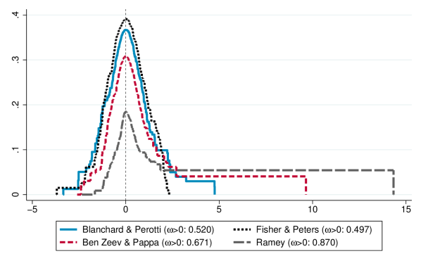
Figure 1: Estimated causal weight functions $\omega_{X}$ for government spending shocks obtained from the replication files for Ramey (2016), quarterly data. Horizontal axis in units of standard deviations. “$\omega>0$:” total weight $\int_{0}^{\infty}\omega_{X}(x)\,dx$ on positive shocks. Papers referenced: Blanchard and Perotti (2002), Fisher and Peters (2010), Ben Zeev and Pappa (2017), Ramey (2011).

Parametric nonlinear specifications.

If one suspects that the average structural function $\Psi_{h}$ is nonlinear, it seems natural to model the nonlinearity directly, rather than to stick to a linear specification as in (7). For example, Jordà (2005) and Jordà and Taylor (2024) suggest including powers of the shock in local projections. Similarly, there is a rich literature on nonlinear extensions of VAR models, see for example Kilian and Lütkepohl (2017, Chapter 18). Such direct modeling of the nonlinearities is sensible if the goal of the analysis is to directly characterize the extent and types of nonlinearity present in the data, e.g., threshold effects or sign and size dependence (Caravello and Martínez Bruera, 2024).

However, for estimating average causal effects, simple linear local projections or VARs appear more robust than nonlinear parametric specifications. As shown in Proposition 1, the linear specification in (7) is robust to misspecification in that it estimates a well-defined average marginal effect regardless of the form of nonlinearity in the structural function $\Psi_{h}$. By contrast, we now show that this is not the case for a local projection specification that includes a quadratic term, suggesting that nonlinear specifications do not generally have such a robustness property.

Consider a quadratic local projection of $Y_{t+h}$ on $X_{t}$, $X_{t}^{2}$, and an intercept. Assume for analytical simplicity that $X_{t}$ has a standard normal distribution, so in particular $X_{t}$ and $X_{t}^{2}$ are uncorrelated (our qualitative conclusions can be shown to go through without the normality assumption). Then the population version of the projection is

$$Y_{t+h}=\beta_{0,h}+\beta_{1,h}X_{t}+\beta_{2,h}X_{t}^{2}+\text{residual}_{h,t+h},$$

with implied derivative of the regression function at $X_{t}=x$ given by

$$\bar{\beta}_{h}(x)\equiv\beta_{1,h}+2\beta_{2,h}x,$$ (10)

and population regression coefficients

$$\beta_{1,h}\equiv\frac{\operatorname*{Cov}(g_{h}(X_{t}),X_{t})}{\operatorname*{Var}(X_{t})},\quad\beta_{2,h}\equiv\frac{\operatorname*{Cov}(g_{h}(X_{t}),X_{t}^{2})}{\operatorname*{Var}(X_{t}^{2})}.$$ (11)

Proposition 2.

Assume that $X_{t}\sim N(0,1)$, and that $g_{h}$ defined in (5) is differentiable with a derivative that is locally absolutely continuous on $\mathbb{R}$. Finally, assume $E[\lvert g_{h}(X_{t})\rvert+\lvert g_{h}^{\prime}(X_{t})\rvert+\lvert g_{h}^{\prime\prime}(X_{t})\rvert]<\infty$. Then, using the definitions (10)–(11),

$$\bar{\beta}_{h}(x)=E[(1+X_{t}x)g_{h}^{\prime}(X_{t})]=E[g_{h}^{\prime}(X_{t})]+xE[g_{h}^{\prime\prime}(X_{t})].$$ (12)

The first expression in (12) shows that the estimated derivative $\bar{\beta}_{h}(x)$ equals a weighted average of the true derivative function $g_{h}^{\prime}(\cdot)$, but with weights that are negative whenever $1+X_{t}x<0$. If the true regression function $g_{h}$ is in fact quadratic, then $\overline{\beta}_{h}(x)$ is consistent for the marginal effect function $\Psi_{h}^{\prime}(x)$. But if the regression function is misspecified, the negative weighting leads to a sign reversal: the second expression in (12) implies that even if $g_{h}$ is monotonically increasing, the estimated derivative $\bar{\beta}_{h}(x)$ will be negative for sufficiently large $x$ whenever $E[g_{h}^{\prime\prime}(X)]<0$. Such sign reversal is not shared by the linear estimator (7), for which the weighting scheme $\omega_{X}$ is convex.

State-dependent specifications.

A particularly popular nonlinear local projection specification in applied work is a state-dependent specification that interacts the shock with a binary regime indicator $S_{t}\in\{0,1\}$ (see Gonçalves, Herrera, Kilian, and Pesavento, 2024, and references therein):

$$Y_{t+h}=\hat{\beta}_{0,h}(1-S_{t})X_{t}+\hat{\beta}_{1,h}S_{t}X_{t}+\hat{\gamma}_{0,h}^{\prime}(1-S_{t})\bm{\mathbf{W}}_{t}+\hat{\gamma}_{1,h}^{\prime}(S_{t}\bm{\mathbf{W}}_{t})+\text{residual}_{h,t+h}.$$

For example, $S_{t}$ may indicate whether the economy is in an NBER recession or not. Assuming that the local projection is fully interacted as above (i.e., all control variables $\bm{\mathbf{W}}_{t}$ are interacted with $S_{t}$), then the procedure is tantamount to running separate regressions on the subsamples with $S_{t}=0$ and $S_{t}=1$, respectively. It follows that all the analysis surrounding Proposition 1 above applies upon conditioning on $S_{t}=s\in\{0,1\}$. In particular, the probability limit of the state-dependent impulse response estimate $\hat{\beta}_{s,h}$ equals a positively weighted average of conditional marginal effects $\partial E[Y_{t+h}\mid X_{t}=x,S_{t}=s]/\partial x$, which have a clear causal interpretation provided the shock independence assumption (2) holds conditional on $S_{t}$ (i.e., within each regime). Thus, despite their apparent linearity conditional on regime, state-dependent local projections identify causal estimands even when the true DGP has a nonlinear form, such as a model with smooth or discrete regime-switching. However, consistent with the discussion in Section 2, it is important to interpret the impulse responses as averaging over all future shocks, including potential future regime switches. In other words, the local projection estimand does not hold the regime fixed within the impulse response horizon.

3.2 Identification with proxies

In many applications, observations of the shock are contaminated by measurement error, such as when accurate measurements are available only in a subset of the time periods. In such cases, researchers typically treat the measurements $Z_{t}$ as a proxy for the shock of interest $X_{t}$, or, equivalently, an instrument for the shock (see Stock and Watson, 2018, for a review). We now show that when the structural function is nonlinear, linear VARs and local projections onto the proxy identify average marginal effects up to scale, provided that the conditional mean of the proxy given the shock is monotone in the shock.

We assume that the proxy $Z_{t}$ is valid, in the sense that it satisfies the exclusion restriction

$$E[Y_{t+h}\mid X_{t},Z_{t}]=E[Y_{t+h}\mid X_{t}]=g_{h}(x),$$ (13)

which formalizes the notion that if we in fact observed the true shock $X_{t}$, the proxy $Z_{t}$ would not provide any further explanatory power for the outcome. It is implied by the standard assumption in the measurement error literature that the measurement error in $Z_{t}$ is non-differential, i.e., that the whole conditional distribution of $Y_{t+h}$ given $(X_{t},Z_{t})$ depends only on $X_{t}$ (or equivalently that $Z_{t}$ is independent of $\bm{\mathbf{U}}_{t+h}$) (e.g., Carroll, Ruppert, Stefanski, and Crainiceanu, 2006, Chapter 2.6).

We consider the “reduced-form” local projection of the outcome $Y_{t+h}$ on the proxy $Z_{t}$. Under (13), the population version of this regression has slope coefficient

$$\tilde{\beta}_{h}\equiv\frac{\operatorname*{Cov}(\zeta(X_{t}),g_{h}(X_{t}))}{\operatorname*{Var}(Z_{t})},$$ (14)

where

$$\zeta(x)\equiv E[Z_{t}\mid X_{t}=x]$$ (15)

denotes the “first-stage” conditional mean function. As shown by Plagborg-Møller and Wolf (2021), this $\tilde{\beta}_{h}$ also corresponds to the probability limit of an impulse response from a structural VAR where the proxy is ordered first, and the specification controls for sufficiently many lags.

Proposition 3.

Assume that $X_{t}$ is continuously distributed on an interval $I\subseteq\mathbb{R}$ (the interval may be unbounded, and could equal $\mathbb{R}$), and that the variance of $Z_{t}$ is positive and finite. Assume that the conditional mean $g_{h}$ defined in (5) is locally absolutely continuous on $I$, and $E[\lvert g_{h}(X)\rvert(1+\lvert\zeta(X)\rvert)]<\infty$. Finally, assume that for sufficiently large positive and negative $x$, the sign of $\zeta(x)-E[Z_{t}]$ does not change, and that $\int_{I}\lvert\tilde{\omega}_{Z}(x)g_{h}^{\prime}(x)\rvert\,dx<\infty$, where

$$\tilde{\omega}_{Z}(x)\equiv\frac{\operatorname*{Cov}(\operatorname{\mathbbm{1}}\{X_{t}\geq x\},\zeta(X_{t}))}{\operatorname*{Var}(Z_{t})}.$$ (16)

Then, the proxy estimand (14) satisfies

$$\tilde{\beta}_{h}=\int_{-\infty}^{\infty}\tilde{\omega}_{Z}(x)g_{h}^{\prime}(x)\,dx.$$

The weight function $\tilde{\omega}_{Z}$ has the following properties:

1. It is invariant to additive and multiplicative measurement error, up to scale: If $\tilde{Z}_{t}=V_{1t}+V_{2t}Z_{t}$, where $(V_{1t},V_{2t})$ is a bivariate random vector independent of $(X_{t},Z_{t})$, then $\tilde{\omega}_{\tilde{Z}}(x)=E[V_{2t}]\tilde{\omega}_{Z}(x)$ for all $x$.

2. It is nonnegative, $\tilde{\omega}_{Z}(x)\geq 0$, provided that $E[Z_{t}\mid X_{t}\geq x]\geq E[Z_{t}\mid X_{t}<x]$.

3. It depends only on the joint distribution of $(X_{t},Z_{t})$, but not on the conditional distribution of $Y_{t+h}$ given $X_{t}$.

A sufficient condition for property (ii) is that the conditional mean function $\zeta(x)$ is monotone increasing. Under this assumption, $\tilde{\omega}_{Z}$ is also hump-shaped: monotonically increasing from 0 to its maximum for $x\leq x_{0}$, and then monotonically decreasing back to 0 for $x\geq x_{0}$, where $x_{0}\equiv\inf\{x\in I\colon\zeta(x)\geq E[Z_{t}]\}$.

Combining Proposition 3 with the identification result (6) implies that linear proxy regressions identify weighted averages of marginal effects, $\theta_{h}(\tilde{\omega}_{Z})=\int\tilde{\omega}_{Z}(x)\Psi_{h}^{\prime}(x)\,dx$, just as in the case of directly observed shocks. Unlike in the observed shocks case, the weights $\tilde{\omega}_{Z}$ will not be positive unless the proxy satisfies the condition in point (ii) of Proposition 3—this condition is slightly weaker than monotonicity of $\zeta(x)$. However, monotonicity of $\zeta$ ensures not just that the weights are positive, but also that they have an intuitive hump-shape, giving most weight to shocks in the middle of the distribution.

Monotonicity of $\zeta$ is implied by, but much weaker than the continuous-treatment version of the Imbens and Angrist (1994) monotonicity condition, needed for causal interpretation of two-stage least squares estimands under endogeneity. We defer the details to Section A.2, where we generalize the identification results in Angrist, Graddy, and Imbens (2000) by allowing for non-smooth potential outcome functions and non-binary $Z_{t}$. It follows from this identification result that monotonicity of $\zeta$ holds under much weaker conditions than those required for causal interpretation of $\tilde{\beta}_{h}$ under endogeneity. Rambachan and Shephard (2021, Theorem 7) derive an alternative characterization of the proxy estimand (14) involving derivatives of the reduced-form potential outcome as a function of the proxy $Z_{t}$ (rather than of the shock $X_{t}$), and therefore the monotonicity assumption has no counterpart in their analysis.

A practical implication of Proposition 3 is that applied researchers should seek to construct proxies that are credibly positively related to the unobserved latent shock of interest. However, it is not essential that the relationship is linear or indeed of any particular known functional form.

Example 2.

An interesting example of a proxy is one constructed from so-called “narrative sign restrictions”, where it is assumed that the researcher observes not the shock itself, but a discrete signal of whether a large shock occurred. While Antolín-Díaz and Rubio-Ramírez (2018) and Giacomini, Kitagawa, and Read (2023) exploit such restrictions in a likelihood framework, Plagborg-Møller and Wolf (2021) and Plagborg-Møller (2022) recommend treating them as a special case of proxy identification.

As a concrete example, assume that for some constants $c_{1},c_{2}\geq 0$ (which may be unknown to the econometrician), $Z_{t}=\operatorname{\mathbbm{1}}\{X_{t}\geq c_{2}\}-\operatorname{\mathbbm{1}}\{X_{t}\leq-c_{1}\}$. That is, the proxy equals 1 for sufficiently large positive shocks, $-1$ for sufficiently large negative shocks, and is otherwise uninformative. Let $F_{X}(x)\equiv P(X_{t}\leq x)$ be the cumulative distribution function (CDF) of $X_{t}$. Then the weight function $\tilde{w}_{Z}(x)$ is nonnegative and proportional to

$$\operatorname*{Cov}(\operatorname{\mathbbm{1}}\{X_{t}\geq x\},Z_{t})=\begin{cases}F_{X}(x)[2-F_{X}(c_{2})-F_{X}(-c_{1})]&\text{for }x\leq-c_{1},\\ F_{X}(x)[1-F_{X}(c_{2})-F_{X}(-c_{1})]+F_{X}(-c_{1})&\text{for }x\in(-c_{1},c_{2}),\\ [1-F_{X}(x)][F_{X}(c_{2})+F_{X}(-c_{1})]&\text{for }x\geq c_{2},\end{cases}$$

as can be verified through direct calculation. It is easy to see that the above weight function is hump-shaped: monotonically increasing until either $x=-c_{1}$ or $x=c_{2}$ (depending on the sign of $1-F_{X}(c_{2})-F_{X}(-c_{1})$), and then monotonically decreasing. Arguably, such a weight function is economically sensible. In fact, if $1-F_{X}(c_{2})=F_{X}(-c_{1})$ (as would be the case if $c_{1}=c_{2}$ and the distribution of $X_{t}$ were symmetric around 0), then the weight function is “nearly” uniform as it is shaped like a plateau: increasing for $x<-c_{1}$, then flat for $x\in[-c_{1},c_{2}]$, then decreasing.

This example shows that conventional proxy local projections or VARs can estimate meaningful causal summaries even if the proxy (which here is discrete) is quite nonlinearly related to the true (continuous) shock, and in ways that are not directly known to the econometrician. This robustness may not be shared by likelihood-based approaches to identification via narrative restrictions.

The weight function (16) does not integrate to 1 due to attenuation bias, so that we only identify average marginal effects up to scale. However, since the weight function doesn’t depend on the outcome, this is not an issue in practice: we can scale $\tilde{\beta}_{h}$ by the response of some normalization variable to the proxy (this is the so-called unit effect normalization) to identify a relative marginal effect. The local projection instrumental variable estimator of Stock and Watson (2018), which is a two-stage least squares version of local projection, automatically performs this normalization.

Since the shock $X_{t}$ is not directly observed, we cannot generally estimate the weight function $\tilde{\omega}_{Z}$ in the data. Instead, it may be useful to plot the observed-shock weight function (9) pretending that $Z_{t}$ is the actual shock of interest. If it happens that $Z_{t}\approx X_{t}$, then these weights will be close to the proxy weights $\tilde{\omega}_{Z}$, so the plot provides a “best-case” scenario.

3.3 Identification with control variables

In applications where it is challenging to isolate purely exogenous shifts in policy or fundamentals, researchers may be willing to assume that the observed variable $X_{t}$ (which could be a policy instrument) is exogenous conditional on some control variables $\bm{\mathbf{W}}_{t}$ (such as variables that comprise the policy-makers information set):

$$X_{t}\mathchoice{\mathrel{\hbox to0.0pt{$\displaystyle\perp$\hss}\mkern 2.0mu{\displaystyle\perp}}}{\mathrel{\hbox to0.0pt{$\textstyle\perp$\hss}\mkern 2.0mu{\textstyle\perp}}}{\mathrel{\hbox to0.0pt{$\scriptstyle\perp$\hss}\mkern 2.0mu{\scriptstyle\perp}}}{\mathrel{\hbox to0.0pt{$\scriptscriptstyle\perp$\hss}\mkern 2.0mu{\scriptscriptstyle\perp}}}\bm{\mathbf{U}}_{h,t+h}\mid\bm{\mathbf{W}}_{t}.$$ (17)

This is a selection on observables assumption as in Angrist and Kuersteiner (2011) and Angrist, Jordà, and Kuersteiner (2018). For example, the assumption holds if $X_{t}=\Upsilon(\varepsilon_{t},\bm{\mathbf{W}}_{t})$, where $\varepsilon_{t}$ is a shock that is independent of $(\bm{\mathbf{W}}_{t}^{\prime},\bm{\mathbf{U}}_{h,t+h}^{\prime})^{\prime}$, a nonparametric version of the recursive (or Cholesky) assumption in linear structural VAR identification (e.g., Christiano, Eichenbaum, and Evans, 1999). Then the conditional expectation function

$$g_{h}(x,\bm{\mathbf{w}})\equiv E[Y_{t+h}\mid X_{t}=x,\bm{\mathbf{W}}_{t}=\bm{\mathbf{w}}]$$

equals the conditional average structural function in the causal model (1):

$$g_{h}(x,\bm{\mathbf{w}})=E[\varphi_{h}(x,\bm{\mathbf{U}}_{h,t})\mid\bm{\mathbf{W}}_{t}=\bm{\mathbf{w}}]\equiv\Psi_{h}(x,\bm{\mathbf{w}}),$$

where the expectation is taken with respect to the conditional distribution of the nuisance shocks $\bm{\mathbf{U}}_{h,t}$ given $\bm{\mathbf{W}}_{t}$.

Even under the selection on observables assumption (17), the local projection with controls (7) need not estimate an average marginal effect if the relationship between $X_{t}$ and the controls is nonlinear. This result extends to recursively identified structural VARs, due to the nonparametric equivalence between these procedures (Plagborg-Møller and Wolf, 2021). Proposition 7 below shows that the population local projection coefficient $\beta_{h}$ can still be written as a weighted average of the marginal effects $\partial g(x,\bm{\mathbf{w}})/\partial x=\partial\Psi_{h}(x,\bm{\mathbf{w}})/\partial x$, but the weights can be negative if the true “propensity score” $\pi^{*}(\bm{\mathbf{w}})\equiv E[X_{t}\mid\bm{\mathbf{W}}_{t}=\bm{\mathbf{w}}]$ is nonlinear. We leave the details, which extend the analysis of Goldsmith-Pinkham, Hull, and Kolesár (2024) to cases with non-discrete $X_{t}$, to Section 6. As usual, negative weights are worrying, as they may lead to a sign-reversal. Hence, in cases where control variables are used for identification, we recommend that researchers do careful sensitivity analysis with respect to both the set of controls and the functional form for the controls (e.g., whether they are included only linearly in the regression or more flexibly by, say, including interactions and polynomials). If $\bm{\mathbf{W}}_{t}$ just consists of a set of mutually exclusive dummies, then linearity of the propensity score comes for free, and the weights are guaranteed to be positive.

4 The bad: identification via heteroskedasticity

Identification via heteroskedasticity has become a popular procedure for causal identification in applications where direct shock measures are unavailable, following Sentana and Fiorentini (2001), Rigobon (2003), and Rigobon and Sack (2004). In a pair of highly-cited papers, Lewbel (2012, 2018) exploits this idea to achieve identification in cross-sectional regressions with endogenous variables and no external instruments (see also Klein and Vella, 2010, for a related approach). In stark contrast to Section 3, the results in this section deliver bad news regarding the sensitivity of identification approaches via heteroskedasticity to the assumption that the underlying structural function is linear: the Rigobon-Sack-Lewbel estimator does not generally estimate average marginal effects; more generally, we show that the nonparametric analogue of the identification approach yields very large identified sets for causal effects. One piece of positive news is that it is possible to test the linearity assumption in the data.

4.1 Nonparametric version of the identification approach

To explain the sensitivity of conventional identification via heteroskedasticity to the linearity assumption on the structural function, it is helpful to first lay out a nonparametric version of the framework before we review the linear case. Since this section is mainly concerned with giving examples of how the identification approach can fail, we specialize the dynamic set-up from Section 2 to a simpler static model.

Nonparametric setup.

We observe an $n$-dimensional vector $\bm{\mathbf{Y}}$ of variables that are nonlinearly related to a latent, scalar shock of interest $X$ as well as an $(m-1)$-dimensional latent vector $\bm{\mathbf{U}}$ of nuisance shocks:

$$\bm{\mathbf{Y}}=\bm{\mathbf{\psi}}(X,\bm{\mathbf{U}}),\quad X\mathchoice{\mathrel{\hbox to0.0pt{$\displaystyle\perp$\hss}\mkern 2.0mu{\displaystyle\perp}}}{\mathrel{\hbox to0.0pt{$\textstyle\perp$\hss}\mkern 2.0mu{\textstyle\perp}}}{\mathrel{\hbox to0.0pt{$\scriptstyle\perp$\hss}\mkern 2.0mu{\scriptstyle\perp}}}{\mathrel{\hbox to0.0pt{$\scriptscriptstyle\perp$\hss}\mkern 2.0mu{\scriptscriptstyle\perp}}}\bm{\mathbf{U}},$$ (18)

where we suppress time subscripts to ease notation. The above model is a (static) nonparametric factor model, since we do not impose parametric restrictions on the unknown structural function $\bm{\mathbf{\psi}}\colon\mathbb{R}^{m}\to\mathbb{R}^{n}$.

The econometrician observes a scalar $D$ that is informative about the heteroskedasticity of the shock of interest $X$ but independent of the nuisance shocks $\bm{\mathbf{U}}$ (jointly with $X$):

$$(D,X)\mathchoice{\mathrel{\hbox to0.0pt{$\displaystyle\perp$\hss}\mkern 2.0mu{\displaystyle\perp}}}{\mathrel{\hbox to0.0pt{$\textstyle\perp$\hss}\mkern 2.0mu{\textstyle\perp}}}{\mathrel{\hbox to0.0pt{$\scriptstyle\perp$\hss}\mkern 2.0mu{\scriptstyle\perp}}}{\mathrel{\hbox to0.0pt{$\scriptscriptstyle\perp$\hss}\mkern 2.0mu{\scriptscriptstyle\perp}}}\bm{\mathbf{U}}.$$ (19)

This assumption implies that $D$ is a valid proxy for $X$, in the sense that $\bm{\mathbf{Y}}$ and $D$ are independent conditional on $X$. But because the variable $D$ only influences the variance and higher moments of $X$ but not its mean,

$$E[X\mid D]=0,$$ (20)

we cannot use the proxy in local projections as in Section 3.2. For concreteness, it may be useful to think of $D$ as a binary regime indicator, which affects the conditional variance $\operatorname*{Var}(X\mid D)$ but not the conditional mean (20), as in the original work by Rigobon (2003).

If we assume that the structural function $\bm{\mathbf{\psi}}$ is linear, it is possible to achieve identification even if $D$ is unobserved and we relax (19) by allowing $D$ to affect the variances of nuisance shocks. See Bacchiocchi, Bastianin, Kitagawa, and Mirto (2024) and Lewis (2024, Section 3) for excellent reviews. However, since we are only interested in showing how the basic identification approach can fail in a nonparametric context, we maintain the stronger assumptions above. It then follows a fortiori that nonparametric identification is even more challenging under weaker assumptions.

Review of linear identification.

If the structural function $\bm{\mathbf{\psi}}$ in (18) is known to be partially linear, identification of causal effects obtains under an additional relevance assumption. Thus, we temporarily assume that

$$\bm{\mathbf{\psi}}(x,\bm{\mathbf{u}})=\bm{\mathbf{\theta}}x+\bm{\mathbf{\gamma}}(\bm{\mathbf{u}}),$$ (21)

where $\bm{\mathbf{\theta}}$ is the unknown vector of causal effects of $X$, while $\bm{\mathbf{\gamma}}\colon\mathbb{R}^{m-1}\to\mathbb{R}^{n}$ is an unknown function. Following Rigobon and Sack (2004) and Lewbel (2012), construct the scalar instrumental variable

$$Z\equiv(D-E[D])Y_{1},$$ (22)

where $Y_{1}$ is the first element of $\bm{\mathbf{Y}}$. In applications, $Y_{1}$ may be a policy instrument that is known to be strongly related to $X$, though it is also allowed to be correlated with the nuisance shocks. Under the linear model (21) and the identification assumptions (19)–(20), $Z$ satisfies the exogeneity restriction for linear identification in Stock and Watson (2018) since $E[Z\mid\bm{\mathbf{U}}]=0$. In particular, under these assumptions, a regression of $\bm{\mathbf{Y}}$ on $Y_{1}$ using $Z$ as instrument identifies the (relative) causal effects of $X$:

$$\frac{1}{\operatorname*{Cov}(Y_{1},Z)}\operatorname*{Cov}(\bm{\mathbf{Y}},Z)=\frac{1}{\theta_{1}}\bm{\mathbf{\theta}}.$$ (23)

To ensure we are not dividing by zero, we need to additionally assume the relevance conditions that (i) the shock of interest is heteroskedastic across regimes, $\operatorname*{Cov}(X^{2},D)\neq 0$, and (ii) the causal effect of $X$ on $Y_{1}$ is nonzero, $\theta_{1}\neq 0$. For completeness, we review the calculations leading to (23) in Section A.3.

4.2 Fragility under nonlinearity

We now argue that the simple linear identification argument fundamentally cannot be extended to nonparametric contexts.

Nonparametric identified set.

We first show that the nonparametric model of identification via heteroskedasticity yields a large identified set for the causal effects of $X$ on $\bm{\mathbf{Y}}$. To do this, we strengthen the independence and conditional mean assumptions (19)–(20) by imposing a specific model for the relationship between $X$ and $D$:

$$X=\sigma(D)W,\quad\text{where $W,D$, and $\bm{\mathbf{U}}$ are mutually independent,}$$ (24)

$\sigma\colon\mathbb{R}\to\mathbb{R}_{+}$ is a known function, and $W$ has a known distribution that is symmetric around 0. This model would, for example, be consistent with the conditionally Gaussian model $X\mid D\sim N(0,\sigma^{2}(D))$.

Proposition 4.

Assume that $(\bm{\mathbf{Y}},D,W,X,\bm{\mathbf{U}})$ satisfy the nonparametric factor model (18) and identification assumption (24). Then there exists an alternative structural function $\tilde{\bm{\mathbf{\psi}}}\colon\mathbb{R}^{2}\to\mathbb{R}^{n}$ and a scalar random variable $\tilde{U}$ independent of $(W,D,X)$ such that $(\tilde{\bm{\mathbf{Y}}},D)$ has the same joint distribution as $(\bm{\mathbf{Y}},D)$, where

$$\tilde{\bm{\mathbf{Y}}}\equiv\tilde{\bm{\mathbf{\psi}}}(X,\tilde{U}),$$

and such that $\tilde{\bm{\mathbf{\psi}}}(-x,\tilde{u})=\tilde{\bm{\mathbf{\psi}}}(x,\tilde{u})$ for all $x,\tilde{u}$.

The proposition states that the identified set for $\bm{\mathbf{\psi}}$ is so large that it always contains a structural function $\bm{\mathbf{\psi}}(x,\bm{\mathbf{u}})$ that is symmetric in $x$ around 0. In particular, we can never rule out that the average marginal effect $\int\omega(x)(\partial E[\bm{\mathbf{\psi}}(x,\bm{\mathbf{U}})]/\partial x)\,dx$ is zero when the weight function $\omega(x)$ is symmetric around 0. Intuitively, the challenge is that $D$ does not affect the mean of $X$, only higher moments, so—without strong functional form restrictions on the relationship between the outcomes and the shocks—we do not have enough information to sign mean effects of shifts in the latent shock $X$. This holds even though we assume that the econometrician knows exactly how $D$ affects the dispersion of the $X$ distribution. Notice that the construction of the observationally equivalent symmetric structural function in Proposition 4 only relies on a single (scalar) nuisance shock; hence, knowledge about the true number of shocks does not ameliorate the identification failure (see Section 5 for further discussion of this point).

A careful inspection of the proof of Proposition 4 reveals that the result is closely related to a known issue with identification via heteroskedasticity in a linear context: while the variance of the shock of interest $X$ must vary across regimes, we cannot simultaneously allow the impulse responses of $X$ to vary across regimes (see Lewis, 2024, Section 6.1, for a discussion and references). However, in a nonparametric context this problem is even worse, since there is no fundamental distinction between “coefficients” and “shock variances” in a general nonlinear model. A priori restrictions that certain “coefficients” are independent of the regime are only meaningful once we parametrize the model, which complicates the development of an empirically useful nonparametric generalization of the identification approach.

Sensitivity of linear procedures.

Because the nonparametric identified set is large, we can expect estimation procedures based on linearity of the structural function to fail to estimate causal objects in general. The next result implies that this is indeed the case for the linear instrumental variable estimator (23) of Rigobon and Sack (2004) and Lewbel (2012).

Proposition 5.

Assume the additively separable structural model

$$\bm{\mathbf{Y}}=\bm{\mathbf{\theta}}(X)+\bm{\mathbf{\gamma}}(\bm{\mathbf{U}}),$$

where $\bm{\mathbf{\theta}}\colon\mathbb{R}\to\mathbb{R}^{n}$, $\bm{\mathbf{\gamma}}\colon\mathbb{R}^{m-1}\to\mathbb{R}^{n}$, and we normalize $E[\bm{\mathbf{\theta}}(X)]=E[\bm{\mathbf{\gamma}}(\bm{\mathbf{U}})]=\bm{\mathbf{0}}$. Suppose that the independence assumption (19) holds, and let $Z$ be given by (22). Suppose that the variables $(\bm{\mathbf{Y}},Z,D)$ have finite second moments, and that the support of $X$ is given by the interval $I\subseteq\mathbb{R}$ (the interval may be unbounded, and could equal $\mathbb{R}$). Suppose also that for each $j$, $\theta_{j}$ (the $j$-th component of $\bm{\mathbf{\theta}}$) is locally absolutely continuous on $I$, and that for some $\underline{x},\overline{x}\in I$, $\theta_{j}(x)$ is monotone for $x\leq\underline{x}$ and for $x\geq\overline{x}$. Then

$$\operatorname*{Cov}(\bm{\mathbf{Y}},Z)=\int\check{\omega}(x)\bm{\mathbf{\theta}}^{\prime}(x)\,dx,$$

where

$$\check{\omega}(x)\equiv\operatorname*{Cov}\big{(}\operatorname{\mathbbm{1}}\{X\geq x\},\theta_{1}(X)(D-E[D])\big{)}.$$ (25)

Proposition 5 shows that regressing $\bm{\mathbf{Y}}$ onto the instrument $Z$ yields a weighted average of marginal effects, but with a weight function $\check{\omega}(x)$ that cannot be guaranteed to be positive. In fact, the weights even integrate to 0 in some cases, for example if $\theta_{1}(x)=\theta_{1}(-x)$ and the conditional distribution of $X$ given $D$ is symmetric around 0. In such cases, the instrumental variable estimator erroneously estimates a zero causal effect of $X$ on $Y_{j}$ for $j\geq 2$ even if $\theta_{j}(x)=\beta_{j}x$ is a linear function with $\beta_{j}\neq 0$.

The weights can also be negative—and therefore cause the econometrician to get the sign of the marginal effects wrong—even in the seemingly favorable setting where (unbeknownst to the econometrician) the policy variable $Y_{1}$ simply equals the shock of interest $X$, without any nonlinearity or contamination by nuisance shocks, i.e., $\theta_{1}(x)=x$. Assume in addition, as in Rigobon (2003), that the regime indicator $D\in\{0,1\}$ is binary and $E[X\mid D]=0$. Then a simple calculation shows that the weights in equation 25 equal

$$\check{\omega}(x)=\operatorname*{Var}(D)\int_{x}^{\infty}[f_{X|1}(v)-f_{X|0}(v)]v\,dv=\operatorname*{Var}(D)\int_{-\infty}^{x}[f_{X|0}(v)-f_{X|1}(v)]v\,dv,$$ (26)

where $f_{X|d}(x)$ is the density of $X$ conditional on regime $D=d$. Suppose the right (resp., left) tail of the $X$ distribution is fatter (resp., thinner) in regime $D=1$ than in regime $D=0$, meaning that $f_{X|1}(x)>f_{X|0}(x)$ for $x\gg 0$ and $f_{X|0}(x)>f_{X|1}(x)$ for $x\ll 0$. Then it follows from equation 26 that $\check{\omega}(x)>0$ for $x\gg 0$, while $\check{\omega}(x)<0$ for $x\ll 0$. This simple example shows that the instrumental variable estimator can easily generate negative weights, even when it satisfies the exclusion and relevance conditions and the policy variable is linear in the shock. To trust that the weights are positive, we would need to have quite detailed information about the conditional shock density in the two regimes; simple moment restrictions do not suffice.

Intuitively, the problem of negative weights comes about because the Rigobon (2003) and Lewbel (2012) instrumental variable $Z$ defined in (22) fails the proxy monotonicity assumption discussed earlier in connection with Proposition 3. Because the only source of exogenous variation is the regime indicator $D$, and this indicator does not affect the mean of the latent shock $X$ but only higher moments, it is generally impossible to construct any proxy variable that is guaranteed to be monotone in $X$, unless we make strong assumptions about the structural function.

If the model is not additively separable as assumed in Proposition 5, the instrumental variables estimator can exhibit even more pathological behavior, in that it may not equal a weighted average of marginal effects at all. As a simple example, consider a multiplicative model $\bm{\mathbf{Y}}=X\bm{\mathbf{\gamma}}(\bm{\mathbf{U}})$ with $E[\bm{\mathbf{\gamma}}(\bm{\mathbf{U}})]=\bm{\mathbf{0}}$ and impose the independence assumption (19). In that model, $E[\bm{\mathbf{Y}}\mid X]=\bm{\mathbf{0}}$, so the marginal effect function is identically zero, but $\operatorname*{Cov}(\bm{\mathbf{Y}},Z)=\operatorname*{Cov}(X^{2},D)\operatorname*{Cov}(\gamma_{1}(\bm{\mathbf{U}}),\bm{\mathbf{\gamma}}(\bm{\mathbf{U}}))\neq 0$ in general, so the instrument erroneously estimates a nonzero effect.

While we have here restricted our analysis to the particular linear instrumental variable estimation procedure developed by Rigobon and Sack (2004) and Lewbel (2012), in the case of a binary regime $D$ and $n=2$ variables, the linear model is just-identified, so all sensible estimation procedures are equivalent with the instrumental variable estimator.

4.3 Silver lining: Testability of the linearity assumption

While the sensitivity of identification via heteroskedasticity to linearity of the structural function $\bm{\mathbf{\psi}}$ is disheartening, at least the linear model (21) implies testable restrictions if we additionally assume that the shock of interest is invertible, so that it equals a linear function of the observables: $X=\bm{\mathbf{\varsigma}}^{\prime}\bm{\mathbf{Y}}$ for some constant vector $\bm{\mathbf{\varsigma}}\in\mathbb{R}^{n}$. This invertibility assumption is common in structural VAR analysis. Under the independence assumption (19), linear invertibility implies that $D$ and $\bm{\mathbf{Y}}$ are independent conditional on $\bm{\mathbf{\varsigma}}^{\prime}\bm{\mathbf{Y}}$, so that $E[D\mid\bm{\mathbf{Y}}]$ has a single-index structure. This restriction is testable in the data (Stute and Zhu, 2005). Other over-identification tests in the linear model are discussed in the review article by Lewis (2024), though we are not aware of any thorough analysis of the power properties of these tests against general nonlinear alternatives.

5 The ugly: identification via non-Gaussianity

A second approach to identification in linear models in the absence of direct shock measures is to assume that the structural shocks are mutually independent and non-Gaussian; see Gouriéroux, Monfort, and Renne (2017), Lanne, Meitz, and Saikkonen (2017), and the review article by Lewis (2024). Lewbel, Schennach, and Zhang (2024) propose a similar approach to achieve identification in cross-sectional endogenous regressions in the absence of external instruments. An earlier literature outside economics goes by the name independent components analysis (ICA), see Kagan, Linnik, and Rao (1973, Chapter 10), Comon (1994), and the textbook by Hyvärinen, Karhunen, and Oja (2001).

This section delivers ugly news regarding the sensitivity of this identification approach to linearity of the structural function: once the linearity assumption is dropped, the non-Gaussianity assumption is essentially vacuous; as a consequence, estimators based on non-Gaussianity and linearity of the structural function can fail spectacularly even under mild departures from linearity. What is worse, the linearity assumption is untestable in general.

5.1 Nonparametric version of the identification approach

As in Section 4, we consider the nonparametric factor model (18). However, unlike in the case of identification via heteroskedasticity, we now do not observe any additional proxy variables that aid in identifying the latent shocks. Instead, we hope to achieve identification via restrictions on the distributions of the shocks.

Review of linear identification.

Assume temporarily that the number of shocks equals the number of observables, $m=n$, and that the structural function is linear:

$$\bm{\mathbf{\psi}}(x,\bm{\mathbf{u}})=\bm{\mathbf{\beta}}x+\bm{\mathbf{\gamma}}\bm{\mathbf{u}},\quad\bm{\mathbf{\beta}}\in\mathbb{R}^{n},\;\bm{\mathbf{\gamma}}\in\mathbb{R}^{n\times(n-1)}.$$

Assume also the $n$ shocks $(X,U_{1},\dots,U_{n-1})$ are mutually independent, and at most one of these shocks has a Gaussian distribution. We will refer to this model as the linear ICA model. A deep result in probability theory, the Darmois-Skitovich Theorem, says that two nontrivial linear combinations of independent variables cannot themselves be independent, unless all the underlying variables are Gaussian. In the context of the linear ICA model, the theorem implies that any two linear combinations $\bm{\mathbf{\varsigma}}^{\prime}\bm{\mathbf{Y}}$ and $\tilde{\bm{\mathbf{\varsigma}}}^{\prime}\bm{\mathbf{Y}}$ of the data $\bm{\mathbf{Y}}=\bm{\mathbf{\beta}}X+\bm{\mathbf{\gamma}}\bm{\mathbf{U}}$ can be independent if and only if these linear combinations equal two different shocks in the model (up to sign and scale). Hence, the shocks in the model can be identified by searching for those linear combinations of the observed variables that are independent; once we have the shocks, we can then estimate their causal effects. See Hyvärinen, Karhunen, and Oja (2001) and Lewis (2024, Section 4) for reviews of estimation procedures.

The abstract identification argument above can be made less mysterious through a method of moments framework that exploits implications of shock independence for higher moments of the data (Lewis, 2024, Section 4.4). Nevertheless, it is clear from both the abstract argument and the more concrete moment-based approach that linearity of the structural function is being leveraged heavily.

5.2 Fragility under nonlinearity

Nonparametric identified set.

Unfortunately, the mere assumptions that the latent shocks are independent and non-Gaussian provide essentially no identification power in a nonparametric context. The identified set under these assumptions is so large that nearly any function of the data can be labeled a “shock”.

Proposition 6.

Let $\tilde{\bm{\mathbf{Y}}}=\bm{\mathbf{\Upsilon}}(\bm{\mathbf{Y}})$ be a homeomorphic transformation of $\bm{\mathbf{Y}}$, with $j$-th element denoted by $\tilde{Y}_{j}$. For all $j=2,\dots,n$, assume that the quantile function of $\tilde{Y}_{j}$ conditional on $\tilde{Y}_{j-1},\tilde{Y}_{j-2},\dots,\tilde{Y}_{1}$ is continuous in the quantile and the conditioning arguments. Define $\tilde{X}\equiv\tilde{Y}_{1}$, and let $\{\bar{U}_{j}\}_{j=1}^{n-1}$ be mutually independent uniform variables on $[0,1]$ that are also independent of $\tilde{X}$. Then there exists a continuous function $\bar{\bm{\mathbf{\psi}}}\colon\mathbb{R}^{n}\to\mathbb{R}^{n}$ such that the random vector

$$\bar{\bm{\mathbf{Y}}}\equiv\bar{\bm{\mathbf{\psi}}}(\tilde{X},\bar{U}_{1},\dots,\bar{U}_{n-1})$$

has the same distribution as $\bm{\mathbf{Y}}$.

Proposition 6 shows that the nonparametric factor model (18) is very under-identified, even if we restrict the number of latent, independent shocks to equal $m=n$ and impose smoothness on the structural function $\bm{\mathbf{\psi}}$. Indeed, any element of almost any one-to-one transformation $\bm{\mathbf{\Upsilon}}(\bm{\mathbf{Y}})$ of the observables could be construed as a “shock” for some data-consistent choice of structural function $\bm{\mathbf{\psi}}$.

The fundamental issue is that non-Gaussianity of the shocks is a vacuous assumption in the nonparametric setting: it is an innocuous normalization to assume that all shocks have uniform distributions, since we can always nonlinearly transform any shock distribution to the uniform distribution via the quantile function. In other words, we have severe identification failure as in Proposition 6 even if the econometrician knows the exact distributions of each shock. Hence, it is no accident that the identification argument in the ICA and structural VAR literatures relies heavily on the linearity assumption: there is no nonlinear equivalent of the Darmois-Skitovich Theorem.

If we allow for slightly less smoothness of the structural function $\bm{\mathbf{\psi}}$, then the identification problem is even worse. As Gunsilius and Schennach (2023) note, any $n$-dimensional vector $\bm{\mathbf{Y}}$ can be represented as a nonlinear factor model (18) in a single latent shock $X$ (so $m=1$ and $\bm{\mathbf{U}}=\bm{\mathbf{0}}$) using a so-called space-filling curve (e.g., Hilbert curve) construction, though the associated $\bm{\mathbf{\psi}}$ function would not be one-to-one. Hence, without restrictions on the structural function, we cannot rule out that the latent shock of interest $X$ drives all the variation in the $n$ observed variables $\bm{\mathbf{Y}}$. Indeed, given a uniform random variable $U$ on $[0,1]$, we can generate an infinite number of independent uniform random variables $\{V_{j}\}$ from the decimal expansion of $U=0.u^{1}_{1}u_{2}^{1}u_{1}^{2}u_{1}^{3}u_{2}^{2}u_{1}^{3}u_{1}^{4}u_{2}^{3}u_{3}^{2}u_{4}^{1}\dotsb$, and taking $V_{j}\equiv 0.u^{j}_{1}u^{j}_{2}\dotsb$ (and hence an infinite number of independent random variables with arbitrary distributions $F_{j}$ by taking the inverse transform $F_{j}^{-1}(V_{j})$).

Sensitivity of linear procedures.

Due to the nonparametric identification failure, we can expect identification approaches based on non-Gaussianity to be very sensitive to exact linearity in the structural function. The following two simple examples illustrate such sensitivity in two settings where the linearity assumption is untestable. Thus, identification via non-Gaussianity is not only fragile, it is also generally not falsifiable.

Example 3.

Let the two latent shocks $(X,U)$ have a bivariate standard normal distribution. Let the two observed variables be given by

$$Y_{1}\equiv X+U,\quad Y_{2}\equiv\gamma(X-U),$$

for an arbitrary measurable nonlinear function $\gamma\colon\mathbb{R}\to\mathbb{R}$. We can interpret this setting as being almost a linear ICA model, except that the second variable has not been transformed quite correctly. In the above model, $Y_{1}$ and $Y_{2}$ are independent, and $Y_{2}$ has a non-Gaussian distribution. Hence, any linearity-based ICA procedure applied to the data $(Y_{1},Y_{2})$ will erroneously conclude that the first variable equals the first shock and the second variable the second shock (up to the mean). Moreover, there is nothing in the data that can reject the validity of the linear ICA assumptions. Notice the lack of continuity: even if $\gamma(\cdot)$ is only slightly nonlinear, linear ICA procedures will conclude (asymptotically) that the first shock contributes 100% of the variance of $Y_{1}$, even though the true number is 50%.

This example illustrates how getting the transformation of $Y_{2}$ slightly wrong can mess up causal inference about the other variable $Y_{1}$ (which is in fact linear in the true shocks).

Example 4.

Consider a model of the form

$$Y_{1}=X+U,\quad Y_{2}=X+\gamma(U),$$

where $X$ and $U$ are independent latent shocks. Section A.4 gives concrete choices of non-Gaussian distributions of the shocks and a smooth $\gamma(\cdot)$ function such that $Y_{1}$ and $Y_{2}$ are independent and both non-normal. Hence, as in the previous example, any linearity-based ICA procedure applied to the data $(Y_{1},Y_{2})$ will erroneously attribute all variation in $Y_{1}$ to the first shock and all variation in $Y_{2}$ to the second shock. Note that in this example, both of the true shocks $(X,U)$ are non-Gaussian, and the only nonlinearity in the true structural model is the relationship between $Y_{2}$ and $U$.

In conclusion, linearity-based ICA identification procedures can be highly misleading under departures from a linear model, as with identification via heteroskedasticity (but unlike identification with observed shocks or proxies). In fact, the situation is arguably worse than in Section 4, since even arbitrarily small structural nonlinearities can yield large biases, and the linearity assumption is not testable in general.

6 Identification of average marginal effects

Extending the analysis in Section 3, we now consider the problem of estimating average marginal effects with a pre-specified weight function when the shock of interest is observed. We first focus on the case without control variables before extending the analysis to allow for controls.

6.1 Identification without controls

We consider the setup from Section 3.1, but drop time subscripts to make it clearer that our analysis applies to cross-sectional as well as time series settings. Let

$$g(x)\equiv E[Y\mid X=x]$$ (27)

denote the conditional mean function from a nonparametric regression of the scalar outcome $Y$ onto the scalar variable $X$. We do not restrict the marginal distribution of $X$: it can be continuous, discrete, or mixed. Let $I\subseteq\mathbb{R}$ denote a (possibly unbounded) interval that contains the support of $X$. We are interested in summarizing $g$ by reporting its weighted average derivative, weighted by some pre-specified weight function $\omega$. With some abuse of notation, we still denote this weighted average derivative by

$$\theta(\omega)\equiv\int_{I}\omega(x)g^{\prime}(x)\,dx,$$

as in Section 2, even though we don’t require that $g(x)$ corresponds to some structural function. To ensure that this object is well-defined, we assume that $g$ is locally absolutely continuous on $I$. Since (27) only defines $g$ on the support of $X$, this requires us to extend $g$ to all of $I$ in cases when there are gaps in the support of $X$, such as when $X$ is discrete. This can be done by linear interpolation: if $P(X\in(a,b))=0$ for some $(a,b)\subseteq I$, we set $g(x)=(g(b)-g(a))(x-a)/(b-a)+g(a)$ for $x\in(a,b)$. If the distribution of $X$ is discrete, this defines the derivative $g^{\prime}$ as the slope between adjacent support points (and the extension will automatically be locally absolutely continuous provided that the spacing between adjacent support points is bounded away from 0).

A regression-based approach to estimating $\theta(\omega)$ first estimates the entire derivative function $g^{\prime}(\cdot)$ nonparametrically (by, say, series or kernel regression), and then averages it using the weights $\omega$. The next result shows that we can alternatively estimate $\theta(\omega)$ as a weighted average of outcomes, $\theta(\omega)=E[\alpha(X)Y]$, where $\alpha$ is the Riesz representer of the linear functional $g\mapsto\theta(\omega)$.

Lemma 1.

Let $\omega(x)\equiv E[\operatorname{\mathbbm{1}}\{X\geq x\}\alpha(X)]$. Suppose that (i) the support of $X$ is contained in a (possibly unbounded) interval $I\subseteq\mathbb{R}$; (ii) $g$ is locally absolutely continuous on $I$; (iii) $E[\lvert\alpha(X)\rvert(1+\lvert g(X)\rvert)]<\infty$ with $E[\alpha(X)]=0$; and (iv) there exists $x_{0}\in I$ such that $E[\lvert\alpha(X)\int_{x_{0}}^{X}\lvert g^{\prime}(x)\rvert\,dx\rvert]<\infty$. Then

$$E[\alpha(X)g(X)]=\int_{I}\omega(x)g^{\prime}(x)\,dx.$$ (28)

Analogous representations for $\theta(\omega)$ are well-known in the literature if we additionally assume that $X$ is continuously distributed (e.g., Newey and Stoker, 1993, equation 2.6). The representation is usually derived by directly applying integration by parts. Our proof instead generalizes the proof of Stein’s lemma (Stein, 1981, Lemma 1), which allows us to drop the requirement that $X$ is continuously distributed and impose only very mild regularity conditions, which essentially just require that both sides of equation 28 are well-defined. In particular, absolute continuity of $g$ is needed to ensure that $\theta(\omega)$ is well-defined, and in Lemma 4 in Appendix B, we show that if the tails of $\omega$ or the tails of $g$ are monotone, then condition (iv) of Lemma 1 holds provided the integral on the right-hand side of (28) exists.

Lemma 1 gives a recipe for constructing weighting-based estimators of $\theta(\omega)$ for particular choices of weight function $\omega$ by replacing the expectation in equation 28 with a sample average and, if the function $\alpha$ is unknown, replacing $\alpha$ with an estimate. For instance, if $X$ is continuous, and we let $\omega(x)=f_{X}(x)$ correspond to the density of $X$, so that $\theta(\omega)=E[g^{\prime}(X)]$ is the (unweighted) average derivative, the required weighting is given by $\alpha(x)=-f_{X}^{\prime}(x)/f_{X}(x)$, leading to the estimator of Härdle and Stoker (1989) if one uses kernel estimators to estimate the density and its derivative. If the identification condition (6) holds, this estimator will estimate the average causal impact of increasing $X$ by an infinitesimal amount. To estimate the average impact of increasing $X$ by a fixed amount $\delta$ (i.e., the unweighted average causal effect), which corresponds to setting $\omega(x)=\frac{1}{\delta}\int_{x-\delta}^{x}f_{X}(x)\,dx$, let $\alpha(x)=-\frac{f_{X}(x)-f_{X}(x-\delta)}{\delta f_{X}(x)}$, replacing the derivative of the density by a discrete change. If we set $\omega(x)=f^{2}(x)$, so that $\alpha(x)=-2f_{X}^{\prime}(x)$, and we use a leave-one-out kernel estimator for the derivative of the density, we recover the famous density-weighted average derivative estimator of Powell, Stock, and Stoker (1989). Finally, for $\omega(x)=E[\operatorname{\mathbbm{1}}\{X\geq x\}X]$, we simply get $\alpha(x)=x$, and Lemma 1 reduces to Proposition 1: this weighting scheme can be estimated by linear regression. As the proofs of Propositions 1, 2, 3 and 5 reveal, these results are also special cases of Lemma 1.

6.2 Identification with control variables

We now generalize the setup to allow for a vector of controls $\bm{\mathbf{W}}$. Consider the weighted average derivative

$$\theta(\omega)\equiv E\left[\int\omega(x,\bm{\mathbf{W}})g^{\prime}(x,\bm{\mathbf{W}})\,dx\right],$$

where the expectation is over the marginal distribution of $\bm{\mathbf{W}}$, and $g^{\prime}$ is the derivative with respect to $x$ of the conditional mean function $g(x,\bm{\mathbf{w}})\equiv E[Y\mid X=x,\bm{\mathbf{W}}=\bm{\mathbf{w}}]$. To ensure this object is well-defined, we assume that for each $\bm{\mathbf{w}}$, the weights $\omega$ are zero outside the interval $I_{\bm{\mathbf{w}}}$ containing the conditional support of $X$ given $\bm{\mathbf{W}}=\bm{\mathbf{w}}$, and that we can extend $g(\cdot,\bm{\mathbf{w}})$ to $I_{\bm{\mathbf{w}}}$ such that $g(\cdot,\bm{\mathbf{w}})$ is locally absolutely continuous on $I_{\bm{\mathbf{w}}}$, such as by linearly interpolating across any gaps in the support.

Like in the case without covariates, a regression-based estimator of $\theta(\omega)$ first estimates the derivative of the regression function $g^{\prime}(x,\bm{\mathbf{w}})$, and then averages the estimated derivative function using the weights $\omega$ and the marginal distribution of the covariates. The next result shows that we can alternatively estimate $\theta(\omega)$ by taking weighted averages of the outcome.

Lemma 2.

Let $\omega(x,\bm{\mathbf{w}})\equiv E[\operatorname{\mathbbm{1}}\{X\geq x\}\alpha(X,\bm{\mathbf{W}})\mid\bm{\mathbf{W}}=\bm{\mathbf{w}}]$. Suppose that conditional on $\bm{\mathbf{W}}$, the following holds almost surely: (i) the support of $X$ is contained in a (possibly unbounded) interval $I_{\bm{\mathbf{W}}}\subseteq\mathbb{R}$; (ii) $g(\cdot,\bm{\mathbf{W}})$ is locally absolutely continuous on $I_{\bm{\mathbf{W}}}$; and (iii) $E[\alpha(X,\bm{\mathbf{W}})\mid\bm{\mathbf{W}}]=0$. Suppose also that (iv) there exists a function $x_{0}(\bm{\mathbf{W}})\in I_{\bm{\mathbf{W}}}$ such that $E[\lvert\alpha(X,\bm{\mathbf{W}})\int_{x_{0(\bm{\mathbf{W}})}}^{X}\lvert g^{\prime}(x,\bm{\mathbf{W}})\rvert\,dx\rvert]<\infty$; and that (v) $E[\lvert\alpha(X,\bm{\mathbf{W}})\rvert(1+\lvert g(X,\bm{\mathbf{W}})\rvert)]<\infty$. Then

$$E\left[\int\omega(x,\bm{\mathbf{W}})g^{\prime}(x,\bm{\mathbf{W}})\,dx\right]=E\left[\alpha(X,\bm{\mathbf{W}})g(X,\bm{\mathbf{W}})\right].$$ (29)

As discussed in Section 6.1, the representation (29) is well-known if the distribution of $X$ is continuous conditional on $\bm{\mathbf{W}}$. The novelty of Lemma 2 is to drop the continuity requirement and relax the regularity conditions.

If $X\in\{0,1\}$ is a binary treatment variable, and we additionally assume that $X$ is as good as randomly assigned conditional on $\bm{\mathbf{W}}$, then $g(1,\bm{\mathbf{w}})-g(0,\bm{\mathbf{w}})$ corresponds to the conditional average treatment effect (ATE) for individuals with $\bm{\mathbf{W}}=\bm{\mathbf{w}}$. In this case, the average derivative simplifies to

$$\theta(\omega) =E\left[(g(1,\bm{\mathbf{W}})-g(0,\bm{\mathbf{W}}))\int\omega(x,\bm{\mathbf{W}})\,dx\right]$$

$$=E[(g(1,\bm{\mathbf{W}})-g(0,\bm{\mathbf{W}}))\alpha(1,\bm{\mathbf{W}})P(X=1\mid\bm{\mathbf{W}})],$$

which corresponds to a weighted average of conditional ATEs. By letting $\alpha(X,\bm{\mathbf{W}})=X/P(X=1\mid\bm{\mathbf{W}})-(1-X)/P(X=0\mid\bm{\mathbf{W}})$, Lemma 2 recovers the classic result that we can estimate the (unweighted) ATE by inverse probability weighting. If $X$ is continuous with density $f_{X}(x\mid\bm{\mathbf{W}})$ conditional on $\bm{\mathbf{W}}$, letting $\alpha(x,\bm{\mathbf{W}})=-f_{X}^{\prime}(x\mid\bm{\mathbf{W}})/f_{X}(x\mid\bm{\mathbf{W}})$ recovers the average derivative $E[g^{\prime}(X,\bm{\mathbf{W}})]$.

For both of these special cases, there is a wealth of papers studying how to best implement regression-based or weighting-based approaches to estimating $\theta(\omega)$, or combinations of both. Recent influential results in the cross-sectional literature (e.g., Chernozhukov, Escanciano, Ichimura, Newey, and Robins, 2022; Chernozhukov, Chetverikov, Demirer, Duflo, Hansen, Newey, and Robins, 2018) highlight the advantages of combining both approaches using the Neyman orthogonal moment condition

$$\theta(\omega)=E[\mu(X,\bm{\mathbf{W}},g)+\alpha(X,\bm{\mathbf{W}})(Y-g(X,\bm{\mathbf{W}}))],$$ (30)

where $\mu(X,\bm{\mathbf{W}},g)=g(1,\bm{\mathbf{W}})-g(0,\bm{\mathbf{W}})$ for the ATE and $\mu(X,\bm{\mathbf{W}},g)=g^{\prime}(X,\bm{\mathbf{W}})$ for the average derivative. This moment condition is orthogonal in the sense that it is insensitive to small perturbations in $g$, in contrast to the regression-based moment condition $\theta(\omega)=E[\mu(X,\bm{\mathbf{W}},g)]$. As a result, an orthogonal method-of-moments estimator based on (30) that plugs in first-stage estimates of $g$ and $\alpha$ can be viewed as a debiased version of the plug-in estimator utilizing the regression-based moment condition. Actually, the moment condition (30) is not only orthogonal, but also doubly robust—insensitive to large perturbations in either $g$ or $\alpha$ so that the orthogonal method-of-moments estimator remains consistent so long as any one of the first-stage estimators is consistent for $\alpha$ or $g$, even if the other estimator is inconsistent. For the binary treatment case, the orthogonal method-of-moments estimator corresponds to the classic augmented inverse probability weighted estimator of Robins, Rotnitzky, and Zhao (1994).

For i.i.d. data, a popular alternative to the orthogonal method-of-moments estimator is to use cross-fitting (Chernozhukov, Escanciano, Ichimura, Newey, and Robins, 2022; Chernozhukov, Chetverikov, Demirer, Duflo, Hansen, Newey, and Robins, 2018). This allows for regularity conditions that are weak enough to accommodate a variety of first-step estimators of $\alpha$ and $\gamma$, including kernels, series, as well as lasso, random forests, or other machine learning estimators, provided that these estimators converge sufficiently fast. Because of this flexibility, the approach is known as debiased machine learning. Recent work by Chernozhukov, Newey, and Singh (2022) and Hirshberg and Wager (2021) develops alternatives to this approach that bypass the need to explicitly estimate the Riesz representer $\alpha$.

These approaches all deliver estimators of $\theta(\omega)$ that converge, under appropriate regularity conditions, at the usual parametric rate (square root of sample size) even if the first-stage estimators are based on complicated nonparametric or machine learning algorithms. Adapting these approaches to time series contexts with dependent data is an interesting area for future research. But one may worry that even in the absence of covariates, given the small sample sizes typically available in macroeconomic applications, estimates of average marginal effects relying on machine-learning or nonparametric first-step estimates of the shock density and the structural function may yield estimates that are too noisy and sensitive to the choice of first-stage tuning parameters. When covariates are needed to argue that the observed variable $X$ is exogenous, the data requirements become even more severe.

The practical challenges associated with fully nonparametric estimation motivates studying what the simple OLS local projection (7) estimates when the true regression function is nonlinear. Extending the analysis of Section 3.3, we now allow the researcher to control for covariates more flexibly by considering the partially linear regression

$$Y=X\beta+\gamma(\bm{\mathbf{W}})+\text{residual},\quad\text{where}\quad\gamma\in\Gamma,$$

and $\Gamma$ is a linear space of control functions. This covers the case with a linear adjustment by letting $\Gamma=\{a+\bm{\mathbf{w}}^{\prime}\bm{\mathbf{b}}\colon a\in\mathbb{R},\bm{\mathbf{b}}\in\mathbb{R}^{\dim(\mathbf{w})}\}$ be the class of linear functions of $\bm{\mathbf{w}}$, as well as the semiparametric partially linear model that lets $\Gamma$ be a large class of “nonparametric” functions. By the projection theorem, the estimand $\beta$ in this regression is given by

$$\beta\equiv\frac{E[(X-\pi(\bm{\mathbf{W}}))g(X,\bm{\mathbf{W}})]}{\operatorname*{Var}(X-\pi(\bm{\mathbf{W}}))},$$ (31)

where $\pi(\bm{\mathbf{W}})\equiv\operatorname*{argmin}_{\gamma_{0}\in\Gamma}E[(X-\gamma_{0}(\bm{\mathbf{W}}))^{2}]$ denotes the projection of $X$ onto $\Gamma$ (if $X$ and $\bm{\mathbf{W}}$ are independent, the estimand (31) reduces to that in (8); we assume the projection exists). We denote the true conditional expectation (the propensity score, if $X$ is binary) by $\pi^{*}(\bm{\mathbf{W}})\equiv E[X\mid\bm{\mathbf{W}}]$.

The next result uses Lemma 2 to generalize Proposition 1 to the case with covariates.

Proposition 7.

Let $\omega^{*}(x,\bm{\mathbf{W}})\equiv E[\operatorname{\mathbbm{1}}\{X\geq x\}(X-\pi^{*}(\bm{\mathbf{W}}))\mid\bm{\mathbf{W}}]$, and suppose $X$ has finite second moments, and that $\operatorname*{Var}(X-\pi(\bm{\mathbf{W}}))>0$. Suppose that either (a) $\pi=\pi^{*}$; or else (b) for some $\gamma_{0},\gamma_{1}\in\Gamma$, and some weights $\lambda(x,\bm{\mathbf{w}})$ such that $\int\lambda(x,\bm{\mathbf{w}})\,dx=\pi^{*}(\bm{\mathbf{w}})+\gamma_{1}(\bm{\mathbf{w}})$, $E[g(X,\bm{\mathbf{W}})\mid\bm{\mathbf{W}}=\bm{\mathbf{w}}]=\gamma_{0}(\bm{\mathbf{w}})+\int\lambda({x},\bm{\mathbf{w}})g^{\prime}(x,\bm{\mathbf{w}})\,dx$ for almost all $\bm{\mathbf{w}}$.

Furthermore, assume that conditional on $\bm{\mathbf{W}}$, the following holds almost surely: (i) the support of $X$ is contained in a (possibly unbounded) interval $I_{\bm{\mathbf{W}}}\subseteq\mathbb{R}$; and (ii) $g(\cdot,\bm{\mathbf{W}})$ is locally absolutely continuous on $I_{\bm{\mathbf{W}}}$. Finally, assume that (iii) $E[\int\lvert\omega^{*}(x,\bm{\mathbf{W}})g^{\prime}(x,\bm{\mathbf{W}})\rvert\,dx]<\infty$ and $E[\lvert g(X,\bm{\mathbf{W}})(X-\pi^{*}(\bm{\mathbf{W}}))\rvert]<\infty$. Then the estimand (31) satisfies

$$\beta=\theta(\omega),\quad\text{where}\quad\omega(x,\bm{\mathbf{W}})\equiv\frac{\omega^{*}(x,\bm{\mathbf{W}})+(\pi^{*}(\bm{\mathbf{W}})-\pi(\bm{\mathbf{W}}))\lambda({x},\bm{\mathbf{w}})}{\operatorname*{Var}(X-\pi(\bm{\mathbf{W}}))},$$

where, if condition (a) holds, we let $\lambda(x,\bm{\mathbf{w}})=0$.

The weights integrate to one: $E[\int\omega(x,\bm{\mathbf{W}})\,dx]=1$. A sufficient condition for the weights to be non-negative is that condition (a) holds, in which case $\omega^{*}(x,\bm{\mathbf{w}})$ is hump-shaped as a function of $x$ for almost all $\bm{\mathbf{w}}$: monotonically increasing from $0$ to its maximum for $x=\pi^{*}(\bm{\mathbf{w}})$, and then monotonically decreasing back to $0$.

To interpret this result, it is useful to first consider the case where the class $\Gamma$ of control functions is rich enough so that condition (a) holds. This is trivially the case, for instance, if $\bm{\mathbf{W}}$ just consists of a single set of fixed effects. In this case, we obtain an analogue of Proposition 1: (partially) linear regression identifies a weighted average of marginal effects, with hump-shaped weights—this holds regardless of the distribution of $X$, be it discrete, continuous or mixed. If the conditional distribution of $X$ given $\bm{\mathbf{W}}$ is continuous, then the weighting $\omega(x,\bm{\mathbf{W}})=\omega^{*}(x,\bm{\mathbf{W}})/\operatorname*{Var}(X-\pi^{*}(\bm{\mathbf{W}}))$ varies smoothly with $x$; if there are mass points, as in the case of a discrete or mixed distribution, then the weight function jumps discontinuously at the mass points. If the treatment $X$ is discrete with support $0,1,\dotsc$, we recover the result in Angrist and Krueger (1999) that regression estimates a weighted average of the causal effects of increasing $X$ by one unit,

$$\beta=\frac{E\left[\sum_{s=1}^{\infty}E[\operatorname{\mathbbm{1}}\{X\geq s\}(X-\pi^{*}(\bm{\mathbf{W}}))\mid\bm{\mathbf{W}}](g(s,\bm{\mathbf{W}})-g(s-1,\bm{\mathbf{W}}))\right]}{E\left[\sum_{s=1}^{\infty}E[\operatorname{\mathbbm{1}}\{X\geq s\}(X-\pi^{*}(\bm{\mathbf{W}}))\mid\bm{\mathbf{W}}]\right]}.$$

Now suppose that condition (a) is violated, because the specification for $\Gamma$ is not sufficiently flexible to model the true propensity score $\pi^{*}(\bm{\mathbf{W}})$. In general, this may lead to omitted variable bias, as the partially linear model may not be sufficiently flexible to account for all confounding due to $\bm{\mathbf{W}}$. Condition (b) prevents this scenario, ensuring that any bias due to confounding is accounted for. As a simple example of when the condition holds, consider the case where the true conditional mean function has a multiplicative form: $g(x,\bm{\mathbf{W}})=Xg^{\prime}(\bm{\mathbf{W}})+\gamma_{0}(\bm{\mathbf{W}})$, with $\gamma_{0}\in\Gamma$. The partially linear model is misspecified, because the marginal effect is not constant, but varies with $\bm{\mathbf{W}}$. But condition (b) holds with $\gamma_{1}(\bm{\mathbf{w}})=0$ and $\lambda(x,\bm{\mathbf{w}})=\pi^{*}(\bm{\mathbf{w}})\varphi(x)$, where $\varphi(x)$ is an arbitrary density function. Because the marginal effect varies only with $\bm{\mathbf{W}}$ but not with $X$, Proposition 7 simplifies to

$$\beta=\frac{E\left[(E[X^{2}\mid\bm{\mathbf{W}}]-\pi(\bm{\mathbf{W}})\pi^{*}(\bm{\mathbf{W}}))g^{\prime}(\bm{\mathbf{W}})\right]}{\operatorname*{Var}(X-\pi^{*}(\bm{\mathbf{W}}))}.$$

If $\pi=\pi^{*}$, we obtain a generalization of the Angrist (1998) result for binary treatments: the weights are proportional to the conditional variance of $X$, $\operatorname*{Var}(X\mid\bm{\mathbf{W}})$. But if $\pi\neq\pi^{*}$, the weight function may be negative for some values of $\bm{\mathbf{W}}$. Consider, for instance, a panel data scenario where $\Gamma$ is linear, and $\bm{\mathbf{W}}$ consists of unit and time fixed effects. Then the assumption $\gamma_{0}\in\Gamma$ amounts to a parallel trends assumption: in the absence of the treatment, the average differences in outcomes for different units are constant and do not depend on the time period. If the treatment effects are heterogeneous, so that $g^{\prime}(\bm{\mathbf{W}})$ depends on the unit and time period, then this two-way fixed effects regression still estimates a weighted average of marginal effects, but with weights that are negative if $E[X^{2}\mid\bm{\mathbf{W}}]<\pi(\bm{\mathbf{W}})\pi^{*}(\bm{\mathbf{W}})$. In the context of a binary treatment and two-way fixed effects regressions, this result has been noted in de Chaisemartin and D’Haultfœuille (2020) and Goodman-Bacon (2021). Proposition 7 generalizes this to an arbitrary treatment distribution and a general regression specification.

Another example where condition (b) of Proposition 7 holds is when $X$ is bounded below by some baseline value (say, 0), $X\geq 0$, and the baseline outcome model is correctly specified, $g(0,\bm{\mathbf{W}})\in\Gamma$. Then condition (b) holds with $\gamma_{0}(\bm{\mathbf{W}})=g(0,\bm{\mathbf{W}})$, $\gamma_{1}=0$, and $\lambda(x,\bm{\mathbf{W}})=P(X\geq x\mid\bm{\mathbf{W}})$. In this case, the weights simplify to $\omega(x,\bm{\mathbf{W}})=E[\operatorname{\mathbbm{1}}\{X\geq x\}(X-\pi(\bm{\mathbf{W}}))\mid\bm{\mathbf{W}}]/\operatorname*{Var}(X-\pi(\bm{\mathbf{W}}))$.

Thus, if the marginal effects are constant, the partially linear model is doubly robust: the regression estimand is consistent for this constant treatment effect so long as either $\pi^{*}\in\Gamma$ or $g(0,\bm{\mathbf{W}})\in\Gamma$, as noted, for instance, in Robins, Mark, and Newey (1992). But this double robustness doesn’t fully extend to the case with heterogeneous marginal effects. If the researcher gets the design (i.e., treatment assignment process) right, in the sense that $\pi=\pi^{*}$, then the partially linear regression estimates an average marginal effect. However, if the researcher gets it wrong, and only gets the outcome model under no treatment right, so that only condition (b) of Proposition 7 holds, then weights on some of the true marginal effects $g^{\prime}(X,\bm{\mathbf{W}})$ may be negative, risking a sign-reversal. This asymmetry has been noted by Goldsmith-Pinkham, Hull, and Kolesár (2024) for the case with a binary treatment $X$. Proposition 7 shows that the result is general. The upshot of this asymmetry is that in cases where the treatment variable $X$ is only conditionally exogenous—whether the data is cross-sectional, panel, or time series—it pays off to conduct a sensitivity analysis with respect to the functional form of the control specification, in addition to the standard sensitivity analysis with respect to the set of controls.

7 Conclusion

We have shown that conventional linear methods for identifying causal effects in applied time series analysis based on observed shocks or proxies are robust to misspecification: they estimate a positively weighted average of the true nonlinear causal effects, irrespective of the extent of nonlinearities in the underlying DGP. By contrast, identification approaches that exploit heteroskedasticity or non-Gaussianity of latent shocks are highly sensitive to violations of the assumed linear functional form of the structural model. Moreover, while linear identification via heteroskedasticity provides some testable restrictions, identification via non-Gaussianity is generally unfalsifiable despite the potential for severe biases.

Our results suggest that it is worthwhile for applied researchers to expend the effort involved in constructing direct measures of shocks, or at least proxies that are credibly (approximately) monotonically related to the latent shock of interest. While shock measurement via narrative approaches or detailed institutional knowledge is admittedly highly work-intensive, it affords an insurance against functional form misspecification which is not matched by the other identification approaches that we analyze. We leave other identification approaches like identification via long-run or sign restrictions for future work.

When reporting impulse responses from linear specifications with observed shocks, we recommend that researchers routinely report the implicit weight function, which is easy to compute via standard regression software. If the weight function associated with conventional local projections or VARs is deemed to be unattractive, it may be possible to reweight the data to provide other causal summaries as discussed in Section 6, though further analysis is required on the best practices for doing so in macroeconomic applications.

More broadly, we hope that our paper will boost the agenda spearheaded by Angrist and Kuersteiner (2011), Angrist, Jordà, and Kuersteiner (2018), and Rambachan and Shephard (2021) that seeks to draw lessons for macroeconometrics from the microeconometric treatment effect literature. The nonparametric framework used in the treatment effect literature contains useful lessons for empirical work in macroeconomics, even though explicit nonparametric estimation or debiased machine learning methods are impractical due to the much smaller data sets typical in macroeconomics.

Appendix A Further results

A.1 Integrals of the weight function

The following lemma provides an identification result for integrals of the causal weight function $\omega_{X}$ defined in Section 3.1.

Lemma 3.

Let $\omega_{X}$ be given by (9). Assume that $E[X_{t}^{2}]<\infty$. Let $\underline{x},\overline{x}$ be constants such that $-\infty\leq\underline{x}<\overline{x}\leq\infty$. Then

$$\int_{\underline{x}}^{\overline{x}}\omega_{X}(x)\,dx=\frac{\operatorname*{Cov}\left(\max\{\min\{X_{t},\overline{x}\},\underline{x}\},X_{t}\right)}{\operatorname*{Var}(X_{t})}.$$

Proof.

By Fubini’s theorem and linearity of the covariance operator,

$$\int_{\underline{x}}^{\overline{x}}\operatorname*{Cov}(\operatorname{\mathbbm{1}}\{X_{t}\geq x\},X_{t})\,dx=\operatorname*{Cov}\left(\int_{\underline{x}}^{\overline{x}}\operatorname{\mathbbm{1}}\{X_{t}\geq x\}\,dx,X_{t}\right).$$

Considering separately the three cases $X_{t}<\underline{x}$, $X_{t}\in[\underline{x},\overline{x}]$, and $X_{t}>\overline{x}$, it can be verified that

$$\int_{\underline{x}}^{\overline{x}}\operatorname{\mathbbm{1}}\{X_{t}\geq x\}\,dx=\max\{\min\{X_{t},\overline{x}\},\underline{x}\}-\underline{x}.\qed$$

Note that the lemma holds even if $X_{t}$ has a discrete distribution (e.g., the empirical distribution). It implies in particular that the OLS-estimated weight function discussed in Section 3.1 integrates to 1 across all $x\in\mathbb{R}$ in finite samples.

A.2 Identification with instruments under endogeneity

We here generalize the setup in Section 3.2 by allowing $X_{t}$ to be endogenous. In particular, we retain the nonparametric structural model (1), but drop the independence assumption (2). Let

$$X_{t}=\xi(Z_{t},V_{t})$$ (32)

denote the first stage equation. We assume that $Z_{t}$ is a valid instrument in the sense that $Z_{t}\mathchoice{\mathrel{\hbox to0.0pt{$\displaystyle\perp$\hss}\mkern 2.0mu{\displaystyle\perp}}}{\mathrel{\hbox to0.0pt{$\textstyle\perp$\hss}\mkern 2.0mu{\textstyle\perp}}}{\mathrel{\hbox to0.0pt{$\scriptstyle\perp$\hss}\mkern 2.0mu{\scriptstyle\perp}}}{\mathrel{\hbox to0.0pt{$\scriptscriptstyle\perp$\hss}\mkern 2.0mu{\scriptscriptstyle\perp}}}(V_{t},\mathbf{U}_{t+h})$. We let

$$\Psi_{h}(x,v)\equiv E[\psi_{h}(x,\bm{\mathbf{U}}_{h,t+h})\mid V_{t}=v]$$

denote the marginal treatment response function. Note that if the shock $X_{t}$ is binary, then the difference $\Psi(1,v)-\Psi(0,v)$ corresponds to the marginal treatment effect of Heckman and Vytlacil (1999, 2005). If the independence assumption (2) holds, then the marginal treatment response function doesn’t depend on $v$, and reduces to the average structural function. Under endogeneity, the population version of the “reduced-form” regression of the outcome $Y_{t+h}$ onto $Z_{t}$ has the slope coefficient

$$\tilde{\beta}_{h}=\frac{E[(Z_{t}-E[Z_{t}])\Psi_{h}(X_{t},{V}_{t})]}{\operatorname*{Var}(Z_{t})}.$$ (33)

As in Section 6.2, we assume that that support of $X_{t}$ conditional on $V_{t}$ is contained in an interval $I_{V_{t}}$. If there are gaps in the support of $X_{t}$, such as when $X_{t}$ is discrete, we assume that we can extend $\Psi_{h}(\cdot,v)$ to $I_{V_{t}}$ such that the extension is locally absolutely continuous.

Applying Lemma 2 with ${V}_{t}$ playing the role of the covariates $\bm{\mathbf{W}}$ then yields the following result:

Proposition 8.

Consider the model in equations 1 and 32, with $Z_{t}\mathchoice{\mathrel{\hbox to0.0pt{$\displaystyle\perp$\hss}\mkern 2.0mu{\displaystyle\perp}}}{\mathrel{\hbox to0.0pt{$\textstyle\perp$\hss}\mkern 2.0mu{\textstyle\perp}}}{\mathrel{\hbox to0.0pt{$\scriptstyle\perp$\hss}\mkern 2.0mu{\scriptstyle\perp}}}{\mathrel{\hbox to0.0pt{$\scriptscriptstyle\perp$\hss}\mkern 2.0mu{\scriptscriptstyle\perp}}}(V_{t},\bm{\mathbf{U}}_{t+h})$. Suppose that $Z_{t}$ has positive and finite variance. Suppose also that conditional on $V_{t}$, the following holds almost surely: (i) the support of $X$ is contained in a (possibly unbounded) interval $I_{V_{t}}\subseteq\mathbb{R}$; and (ii) $\Psi_{h}(\cdot,V_{t})$ is locally absolutely continuous on $I_{V_{t}}$. Suppose also that (iii) there exists a function $x_{0}(V_{t})\in I_{V_{t}}$ such that $E[\lvert(Z_{t}-E[Z_{t}])\int_{x_{0(V_{t})}}^{X_{t}}\lvert\Psi_{h}^{\prime}(x,V_{t})\rvert\,dx\rvert]<\infty$; and that (iv) $E[\lvert\Psi_{h}(X_{t},V_{t})\rvert(1+\lvert Z_{t}\rvert)]<\infty$. Then the estimand (33) satisfies

$$\tilde{\beta}_{h}=E\left[\int\omega(x,V_{t})\Psi_{h}^{\prime}(x,V_{t})\,dx\right],$$

where $\omega(x,v)\equiv E[\operatorname{\mathbbm{1}}\{X_{t}\geq x\}(Z_{t}-E[Z_{t}])\mid V_{t}=v]/\operatorname*{Var}(Z_{t})$.

Proposition 8 shows that the reduced-form regression of $Y_{t}$ onto $Z_{t}$ identifies a weighted average of derivatives of the marginal treatment response function. The result generalizes Theorem 1 of Angrist, Graddy, and Imbens (2000) in several ways: we don’t require differentiability of the potential outcome function $\psi_{h}$, only of the marginal treatment response function; $X_{t}$ is not required to be continuous—it may be discrete or mixed; $Z_{t}$ is not restricted to be binary; we impose no structure on the first-stage equation; and finally, we impose only very weak moment conditions.

A sufficient condition for the weights $\omega(x,v)$ to be positive is the uniform monotonicity condition that $\xi(z,v)$ is increasing in $z$ for almost all $v$: this corresponds to Assumption 4 in Angrist, Graddy, and Imbens (2000) if $z$ is binary. Then, since $\operatorname{\mathbbm{1}}\{\xi(z,v)\geq x\}$ is increasing in $z$, $\omega(x,v)=\operatorname*{Cov}(\operatorname{\mathbbm{1}}\{\xi(Z_{t},v)\geq x\},Z_{t})/\operatorname*{Var}(Z_{t})\geq 0$.

On the other hand, if $X_{t}$ is exogenous, so that $\Psi_{h}^{\prime}(x,v)$ doesn’t depend on $V$, $\tilde{\beta}_{h}$ equals a positively weighted average of marginal effects so long as the weights $\omega$ are positive on average, $E[\omega(x,V_{t})]=\tilde{\omega}_{Z}(x)\geq 0$, rather than for almost all realizations of $V_{t}$. Thus, non-negativity of the weights $\tilde{\omega}_{Z}(x)$ in Proposition 3 is implied by non-negativity of the weights $\omega(x,v)$, but it is clearly a much weaker condition. In particular, as discussed in Section 3.2, it is sufficient that $\zeta(x)=E[Z_{t}\mid X_{t}=x]$ is monotone. This condition holds for many measurement error models for $Z_{t}$, even though the stronger uniform monotonicity condition may be violated.

A.3 Identification via heteroskedasticity: linear case

Here we derive the linear identification result (23), following Rigobon and Sack (2004) and Lewbel (2012). Note first that

$$E[Z\mid\bm{\mathbf{U}}] =E[(\theta_{1}X+\gamma_{1}(\bm{\mathbf{U}}))(D-E[D])\mid\bm{\mathbf{U}}]$$

$$=\theta_{1}E[X(D-E[D])\mid\bm{\mathbf{U}}]+\gamma_{1}(\bm{\mathbf{U}})E[D-E(D)\mid\bm{\mathbf{U}}]$$

$$=\theta_{1}\operatorname*{Cov}(X,D)+\gamma_{1}(\bm{\mathbf{U}})E[D-E(D)]$$

$$=0.$$

Hence,

$$\operatorname*{Cov}(\bm{\mathbf{Y}},Z)=\bm{\mathbf{\theta}}\operatorname*{Cov}(X,Z)+\operatorname*{Cov}(\bm{\mathbf{\gamma}}(\bm{\mathbf{U}}),Z)=\bm{\mathbf{\theta}}\operatorname*{Cov}(X,Z),$$

and the claim (23) follows, provided that $\operatorname*{Cov}(X,Z)\neq 0$. The latter holds if $\theta_{1}\neq 0$ and $\operatorname*{Cov}(X^{2},D)\neq 0$, since

$$\operatorname*{Cov}(X,Z) =E[X(\theta_{1}X+\gamma_{1}(\bm{\mathbf{U}}))(D-E[D])]$$

$$=\theta_{1}\operatorname*{Cov}(X^{2},D)+\operatorname*{Cov}(X,D)E[\gamma_{1}(\bm{\mathbf{U}})]$$

$$=\theta_{1}\operatorname*{Cov}(X^{2},D).\qed$$

A.4 Details for 4

Let $\tilde{U}_{1}$ and $\tilde{U}_{2}$ be independent uniforms on $[0,1]$. By the Box-Muller transform, the two variables

$$\tilde{Y}_{1}\equiv\sqrt{-2\log\tilde{U}_{1}}\cos(2\pi\tilde{U}_{2}),\quad\tilde{Y}_{2}\equiv\sqrt{-2\log\tilde{U}_{1}}\sin(2\pi\tilde{U}_{2}),$$

have a bivariate standard normal distribution.

Define $X\equiv\log(-2\log\tilde{U}_{1})$ and $U\equiv\log\cos^{2}(2\pi\tilde{U}_{2})$, so that $X$ and $U$ are independent and non-Gaussian. By construction, the following two variables are independent:

$$Y_{1}\equiv\log\tilde{Y}_{1}^{2}=X+U,\quad Y_{2}\equiv\log\tilde{Y}_{2}^{2}=X+\gamma(U),$$

where

$$\gamma(u)\equiv\log\left(1-\exp(u)\right),\quad u<0,$$

and we have used that $\exp(U)=\cos^{2}(2\pi\tilde{U}_{2})=1-\sin^{2}(2\pi\tilde{U}_{2})$. Note that in this example, the shocks $X$ and $U$ do not have mean zero as commonly assumed in the literature, but this is easily rectified by just subtracting off their means in the calculations.∎

A.5 Additional empirical estimates of causal weights

Complementing the results for government spending shocks in Figure 1 (Section 3.1), Figures 2, 3 and 4 show estimated causal weight functions for several identified tax shocks, technology shocks, and monetary policy shocks. The data is obtained from the replication files for Ramey (2016), as discussed in Section 3.1. While many of the shocks yield approximately symmetric weight functions, the Romer and Romer (2010) and Mertens and Ravn (2014) tax shocks are both skewed towards tax cuts, while the Christiano, Eichenbaum, and Evans (1999) and Gertler and Karadi (2015) monetary shocks are skewed towards interest rate cuts. As discussed in Section 3.1, this is important to keep in mind when using impulse response estimates to discipline structural models that feature asymmetries.

Empirical weight functions: tax shocks

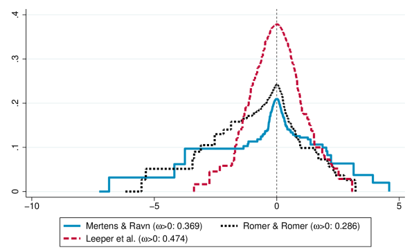
Figure 2: Estimated causal weight functions $\omega_{X}$ for tax shocks obtained from the replication files for Ramey (2016), quarterly data. Horizontal axis in units of standard deviations. “$\omega>0$:” total weight $\int_{0}^{\infty}\omega_{X}(x)\,dx$ on positive shocks. Papers referenced: Mertens and Ravn (2014), Romer and Romer (2010), Leeper, Richter, and Walker (2012).

Empirical weight functions: technology shocks

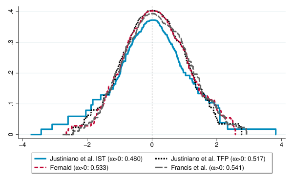
Figure 3: Estimated causal weight functions $\omega_{X}$ for technology shocks obtained from the replication files for Ramey (2016), quarterly data. Horizontal axis in units of standard deviations. “TFP” = total factor productivity. “IST” = investment-specific technology. “$\omega>0$:” total weight $\int_{0}^{\infty}\omega_{X}(x)\,dx$ on positive shocks. Papers referenced: Justiniano, Primiceri, and Tambalotti (2011), Fernald (2014), Francis, Owyang, Roush, and DiCecio (2014).

Empirical weight functions: monetary policy shocks

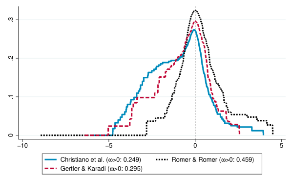
Figure 4: Estimated causal weight functions $\omega_{X}$ for monetary policy shocks obtained from the replication files for Ramey (2016), quarterly data. Horizontal axis in units of standard deviations. “$\omega>0$:” total weight $\int_{0}^{\infty}\omega_{X}(x)\,dx$ on positive shocks. Papers referenced: Christiano, Eichenbaum, and Evans (1999), Romer and Romer (2010), Gertler and Karadi (2015).

Appendix B Proofs

B.1 Auxiliary lemma

Lemma 4.

Suppose that conditions (i)–(iii) of Lemma 1 hold. Suppose additionally that for some $\underline{x},\overline{x}\in I$, $\underline{x}\leq\overline{x}$, it holds that either (a) $\alpha(x)$ only changes sign for $x\in[\underline{x},\overline{x}]$ and $\int_{I}|\omega(x)g^{\prime}(x)|\,dx<\infty$, or (b) $g(x)$ is monotone for $x\leq\underline{x}$ and for $x\geq\overline{x}$. Then condition (iv) of Lemma 1 holds for any $x_{0}\in[\underline{x},\overline{x}]$.

Proof.

Bound

$$E\left[\left|\alpha(X)\int_{x_{0}}^{X}|g^{\prime}(x)|\,dx\right|\right] \leq E[\lvert\alpha(X)\rvert]\int_{\underline{x}}^{\overline{x}}|g^{\prime}(x)|\,dx+E\left[\operatorname{\mathbbm{1}}\{X\geq\overline{x}\}\lvert\alpha(X)\rvert\int_{\overline{x}}^{X}|g^{\prime}(x)|\,dx\right]$$

$$\quad+E\left[\operatorname{\mathbbm{1}}\{X\leq\underline{x}\}\lvert\alpha(X)\rvert\int_{X}^{\underline{x}}|g^{\prime}(x)|\,dx\right].$$

The first term on the right-hand side is finite since $g$ is absolutely continuous on $[\underline{x},\overline{x}]$. Now consider the second term on the right-hand side; the third term can be handled analogously. Under condition (a), $\alpha(x)$ has the same sign for all $x\geq\overline{x}$, so the second term equals

$$\int_{I}\operatorname{\mathbbm{1}}\{x\geq\overline{x}\}\left|E[\operatorname{\mathbbm{1}}\{X\geq x\}\alpha(X)]\right||g^{\prime}(x)|\,dx\leq\int_{I}|\omega(x)||g^{\prime}(x)|\,dx<\infty.$$

Under condition (b), since $g(x)$ is monotone for $x\geq\overline{x}$, the second term on the right-hand side in the first display equals

$$E\left[\operatorname{\mathbbm{1}}\{X\geq\overline{x}\}\lvert\alpha(X)\rvert\left|\int_{\overline{x}}^{X}g^{\prime}(x)\,dx\right|\right] =E\left[\operatorname{\mathbbm{1}}\{X\geq\overline{x}\}\lvert\alpha(X)\rvert\lvert g(X)-g(\overline{x})\rvert\right]$$

$$\leq E[\lvert\alpha(X)g(X)\rvert]+\lvert g(\overline{x})\rvert E[\lvert\alpha(X)\rvert]<\infty.\qed$$

B.2 Proof of Proposition 1

This is a special case of Proposition 3 with $Z=\zeta(X)=X$. Lemma 3 implies that the weights integrate to 1. ∎

B.3 Proof of Proposition 2

Since $g_{h}^{\prime}(x)$ is locally absolutely continuous and $E[\lvert g_{h}^{\prime\prime}(X_{t})\rvert]<\infty$, by Stein’s lemma (Stein, 1981, Lemma 1),

$$E[g_{h}^{\prime\prime}(X_{t})]=E[X_{t}g_{h}^{\prime}(X_{t})].$$

Since $E[\lvert g_{h}(X_{t})\rvert]<\infty$, another application of Stein’s lemma yields $E[X_{t}g_{h}^{\prime}(X_{t})+g_{h}(X_{t})]=E[X_{t}^{2}g_{h}(X_{t})]$. Hence, $\operatorname*{Cov}(g_{h}(X_{t}),X_{t}^{2})=E[X_{t}g_{h}^{\prime}(X_{t})]=E[g_{h}^{\prime\prime}(X_{t})]$. A third application of Stein’s lemma yields $E[g_{h}^{\prime}(X_{t})]=\operatorname*{Cov}(X_{t},g_{h}(X_{t}))$. The result then follows from the definitions (10)–(11). ∎

B.4 Proof of Proposition 3

The representation of the estimand follows directly from Lemmas 1 and 4 with $\alpha(X)=\zeta(X)-E[Z]$. Claim (i) for the weights follows from a simple calculation. Claim (ii) follows from $\operatorname*{Cov}(\operatorname{\mathbbm{1}}\{X_{t}\geq x\},\zeta(X))=\operatorname*{Var}(\operatorname{\mathbbm{1}}\{X_{t}\geq x\})\{E[\zeta(X)\mid X_{t}\geq x]-E[\zeta(X)\mid X_{t}<x]\}$. For the last statement of the proposition, observe that for $x_{U}>x_{L}$, $\tilde{\omega}_{Z}(x_{L})-\tilde{\omega}_{Z}(x_{U})$ is proportional to $E[\operatorname{\mathbbm{1}}\{x_{L}<X_{t}<x_{U}\}(\zeta(X_{t})-E[Z_{t}])]$, which is positive if $x_{0}<x_{L}<x_{U}$ and negative if $x_{L}<x_{U}<x_{0}$. ∎

B.5 Proof of Proposition 4

Let $\tau$ be a Rademacher random variable independent of $(D,W,\bm{\mathbf{U}})$, i.e., $P(\tau=1\mid D,W,\bm{\mathbf{U}})=P(\tau=-1\mid D,W,\bm{\mathbf{U}})=1/2$. Since the distribution of $W$ is symmetric around zero, $W$ has the same distribution as $|W|\times\tau$, and thus $(X,\bm{\mathbf{U}})$ has the same distribution as $(|X|\tau,\bm{\mathbf{U}})$. Let $\tilde{U}$ be uniform on $[0,1]$ independently of $(D,W)$, and let $\phi_{\tau}\colon\mathbb{R}\to\mathbb{R}$ and $\bm{\mathbf{\phi}}_{\bm{\mathbf{U}}}\colon\mathbb{R}\to\mathbb{R}^{m-1}$ be measurable functions such that $(\tau,\bm{\mathbf{U}})$ has the same distribution as $(\phi_{\tau}(\tilde{U}),\bm{\mathbf{\phi}}_{\bm{\mathbf{U}}}(\tilde{U}))$ (see the discussion after Proposition 6 on the construction of such functions). Then it follows that $(X,\bm{\mathbf{U}})$ has the same distribution as $(|X|\phi_{\tau}(\tilde{U}),\bm{\mathbf{\phi}}_{\bm{\mathbf{U}}}(\tilde{U}))$, and the conclusion of the proposition obtains by defining $\tilde{\bm{\mathbf{\psi}}}(x,\tilde{u})\equiv\bm{\mathbf{\psi}}(|x|\phi_{\tau}(\tilde{u}),\bm{\mathbf{\phi}}_{\bm{\mathbf{U}}}(\tilde{u}))$. ∎

B.6 Proof of Proposition 5

Since $\bm{\mathbf{\gamma}}(\bm{\mathbf{U}})$ is independent of $(X,D)$ with mean zero,

$$\operatorname*{Cov}(\bm{\mathbf{Y}},Z\mid X) =\operatorname*{Cov}(\bm{\mathbf{\gamma}}(\bm{\mathbf{U}}),(\theta_{1}(X)+\gamma_{1}(\bm{\mathbf{U}}))(D-E[D])\mid X)$$

$$=\operatorname*{Cov}(\bm{\mathbf{\gamma}}(\bm{\mathbf{U}}),\gamma_{1}(\bm{\mathbf{U}}))\{E[D\mid X]-E[D]\}.$$

The law of total covariance therefore implies

$$\operatorname*{Cov}(\bm{\mathbf{Y}},Z) =E[\operatorname*{Cov}(\bm{\mathbf{Y}},Z\mid X)]+\operatorname*{Cov}(E[\bm{\mathbf{Y}}\mid X],E[Z\mid X])$$

$$=0+E[\bm{\mathbf{\theta}}(X)\{E[Z\mid X]-E[Z]\}].$$

The result now follows from Lemmas 1 and 4, with weights given by

$$\check{\omega}(x) \equiv E[\operatorname{\mathbbm{1}}\{X\geq x\}\{E[Z\mid X]-E[Z]\}]$$

$$=\operatorname*{Cov}(\operatorname{\mathbbm{1}}\{X\geq x\},E[Z\mid X,D])$$

$$=\operatorname*{Cov}(\operatorname{\mathbbm{1}}\{X\geq x\},\theta_{1}(X)(D-E[D])),$$

where the last equality follows from

$$E[Z\mid X,D]=E[Y_{1}\mid X,D](D-E[D])=\theta_{1}(X)(D-E[D]).\qed$$

B.7 Proof of Proposition 6

Let $Q_{j}(\tau\mid\tilde{Y}_{j-1},\tilde{Y}_{j-2},\dots,\tilde{Y}_{1})$ denote the $\tau$-th quantile of $\tilde{Y}_{j}$ conditional on $\tilde{Y}_{j-1},\tilde{Y}_{j-2},\dots,\tilde{Y}_{1}$. Now construct an $n$-dimensional vector $\bm{\mathbf{Y}}^{*}=(Y_{1}^{*},\dots,Y_{n}^{*})$ as follows. First set $Y_{1}^{*}\equiv\tilde{Y}_{1}$. Then for $j>1$, let $Y_{j}^{*}\equiv Q_{j}(\bar{U}_{j-1}\mid\tilde{Y}_{j-1}=Y_{j-1}^{*},\dots,\tilde{Y}_{1}=Y_{1}^{*})$. Standard arguments yield that $\bm{\mathbf{Y}}^{*}$ has the same distribution as $\tilde{\bm{\mathbf{Y}}}$. Consequently, $\bar{\bm{\mathbf{Y}}}\equiv\bm{\mathbf{\Upsilon}}^{-1}(\bm{\mathbf{Y}}^{*})$ has the same distribution as $\bm{\mathbf{Y}}=\bm{\mathbf{\Upsilon}}^{-1}(\tilde{\bm{\mathbf{Y}}})$. The mapping from $(\tilde{X},\bar{U}_{1},\dots,\bar{U}_{n-1})$ to $\bm{\mathbf{Y}}^{*}$ is continuous by the assumptions on $Q_{j}$, and so is the implied $\bar{\bm{\mathbf{\psi}}}$ mapping by continuity of $\bm{\mathbf{\Upsilon}}^{-1}$. ∎

B.8 Proof of Lemma 1

This result follows directly from Lemma 2 by letting $\bm{\mathbf{W}}$ equal a constant. ∎

B.9 Proof of Lemma 2

Observe

$$E\left[\int\omega(x,\bm{\mathbf{W}})g^{\prime}(x,\bm{\mathbf{W}})\,dx\right] =E\left[\int_{I_{\bm{\mathbf{W}}}}E[\operatorname{\mathbbm{1}}\{X\geq x\geq x_{0}(\bm{\mathbf{W}})\}\alpha(X,\bm{\mathbf{W}})\mid\bm{\mathbf{W}}]g^{\prime}(x,\bm{\mathbf{W}})\,dx\right]$$

$$\quad-E\left[\int_{I_{\bm{\mathbf{W}}}}E[\operatorname{\mathbbm{1}}\{X<x<x_{0}(\bm{\mathbf{W}})\}\alpha(X,\bm{\mathbf{W}})\mid\bm{\mathbf{W}}]g^{\prime}(x,\bm{\mathbf{W}})\,dx\right]$$

$$=E\left[\int_{I_{\bm{\mathbf{W}}}}\operatorname{\mathbbm{1}}\{X\geq x\geq x_{0}(\bm{\mathbf{W}})\}\alpha(X,\bm{\mathbf{W}})g^{\prime}(x,\bm{\mathbf{W}})\,dx\right]$$

$$\qquad-E\left[\int_{I_{\bm{\mathbf{W}}}}\operatorname{\mathbbm{1}}\{X<x<x_{0}(\bm{\mathbf{W}})\}\alpha(X,\bm{\mathbf{W}})g^{\prime}(x,\bm{\mathbf{W}})\,dx\right]$$

$$=E\left[\operatorname{\mathbbm{1}}\{X\geq x_{0}(\bm{\mathbf{W}})\}\alpha(X,\bm{\mathbf{W}})(g(X,\bm{\mathbf{W}})-g(x_{0}(\bm{\mathbf{W}}),\bm{\mathbf{W}}))\right]$$

$$\qquad-E\left[\operatorname{\mathbbm{1}}\{X<x_{0}(\bm{\mathbf{W}})\}\alpha(X,\bm{\mathbf{W}})(g(x_{0}(\bm{\mathbf{W}}),\bm{\mathbf{W}})-g(X,\bm{\mathbf{W}}))\right]$$

$$=E\left[\alpha(X,\bm{\mathbf{W}})(g(X,\bm{\mathbf{W}})-g(x_{0}(\bm{\mathbf{W}}),\bm{\mathbf{W}}))\right]$$

$$=E\left[\alpha(X,\bm{\mathbf{W}})g(X,\bm{\mathbf{W}})\right],$$

where the first equality uses the fact that since $E[{\alpha(X,\bm{\mathbf{w}})}\mid\bm{\mathbf{W}}]=0$ by condition (iii), $\omega(x,\bm{\mathbf{w}})=-E[\operatorname{\mathbbm{1}}\{X<x\}\alpha(X,\bm{\mathbf{w}})\mid\bm{\mathbf{W}}=\bm{\mathbf{w}}]$, the second equality uses Fubini’s theorem, which is justified since both integrals exist by condition (iv), the third equality follows by the fundamental theorem of calculus and condition (ii), the fourth equality collects terms, and the last equality uses iterated expectations, which is justified since

$$E\left[\lvert\alpha(X,\bm{\mathbf{W}})g(x_{0}(\bm{\mathbf{W}}),\bm{\mathbf{W}})\rvert\right]$$

$$\leq E\left[\lvert\alpha(X,\bm{\mathbf{W}})g(X,\bm{\mathbf{W}})\rvert\right]+E\left[\lvert\alpha(X,\bm{\mathbf{W}})(g(X,\bm{\mathbf{W}})-g(x_{0}(\bm{\mathbf{W}}),\bm{\mathbf{W}}))\rvert\right]$$

$$\leq E\left[\lvert\alpha(X,\bm{\mathbf{W}})g(X,\bm{\mathbf{W}})\rvert\right]+E\left[\left|\alpha(X,\bm{\mathbf{W}})\int_{x_{0}(\bm{\mathbf{W}})}^{X}\lvert g^{\prime}(x,\bm{\mathbf{W}})\rvert\,dx\right|\right]<\infty,$$

by conditions (iv) and (v). ∎

B.10 Proof of Proposition 7

Observe that under either condition (a) or condition (b),

$$E[(X-\pi(\bm{\mathbf{W}}))g(X,\bm{\mathbf{W}})]$$

$$=E[(X-\pi^{*}(\bm{\mathbf{W}}))g(X,\bm{\mathbf{W}})]+E\left[(\pi^{*}(\bm{\mathbf{W}})-\pi(\bm{\mathbf{W}}))\int\lambda({x},\bm{\mathbf{W}})g^{\prime}(x,\bm{\mathbf{W}})\,dx\right].$$

Applying Lemma 2 with $\alpha(X,\bm{\mathbf{W}})=X-\pi^{*}(\bm{\mathbf{W}})$ and $x_{0}(\bm{\mathbf{W}})=\pi^{*}(\bm{\mathbf{W}})$ yields

$$E[(X-\pi^{*}(\bm{\mathbf{W}}))g(X,\bm{\mathbf{W}})]=E\left[\int\omega^{*}(x,\bm{\mathbf{W}})g^{\prime}(x,\bm{\mathbf{W}})\,dx\right].$$

Note that condition (iv) of Lemma 2 follows from a similar argument as in Lemma 4 (conditional on $\bm{\mathbf{W}}$).

Since

$$\operatorname*{Var}(X-\pi(\bm{\mathbf{W}}))=E[(X-\pi^{*}(\bm{\mathbf{W}}))X]+E[(\pi^{*}(\bm{\mathbf{W}})-\pi(\bm{\mathbf{W}}))\pi^{*}(\bm{\mathbf{W}})]$$

$$=E[(X-\pi^{*}(\bm{\mathbf{W}}))X]+E\left[(\pi(\bm{\mathbf{W}})-\pi^{*}(\bm{\mathbf{W}}))\int\lambda(x,\bm{\mathbf{W}})\,dx\right],$$

it follows that the weights integrate to one. The last statement of the proposition can be shown using the same argument as in the proof of Proposition 3. ∎

References

- (1)
- Angrist (1998) Angrist, J. D. (1998): “Estimating the Labor Market Impact of Voluntary Military Service Using Social Security Data on Military Applicants,” Econometrica, 66(2), 249–288.
- Angrist, Graddy, and Imbens (2000) Angrist, J. D., K. Graddy, and G. W. Imbens (2000): “The Interpretation of Instrumental Variables Estimators in Simultaneous Equations Models with an Application to the Demand for Fish,” Review of Economic Studies, 67(3), 499–527.
- Angrist, Jordà, and Kuersteiner (2018) Angrist, J. D., Ò. Jordà, and G. M. Kuersteiner (2018): “Semiparametric Estimates of Monetary Policy Effects: String Theory Revisited,” Journal of Business & Economic Statistics, 36(3), 371–387.
- Angrist and Krueger (1999) Angrist, J. D., and A. B. Krueger (1999): “Empirical Strategies in Labor Economics,” in Handbook of Labor Economics, ed. by O. C. Ashenfelter, and D. Card, vol. 3, chap. 3, pp. 1277–1366. Elsevier.
- Angrist and Kuersteiner (2011) Angrist, J. D., and G. M. Kuersteiner (2011): “Causal Effects of Monetary Shocks: Semiparametric Conditional Independence Tests with a Multinomial Propensity Score,” Review of Economics and Statistics, 93(3), 725–747.
- Angrist and Pischke (2009) Angrist, J. D., and J.-S. Pischke (2009): Mostly Harmless Econometrics. Princeton University Press.
- Antolín-Díaz and Rubio-Ramírez (2018) Antolín-Díaz, J., and J. F. Rubio-Ramírez (2018): “Narrative Sign Restrictions for SVARs,” American Economic Review, 108(10), 2802–29.
- Bacchiocchi, Bastianin, Kitagawa, and Mirto (2024) Bacchiocchi, E., A. Bastianin, T. Kitagawa, and E. Mirto (2024): “Partially identified heteroskedastic SVARs,” arXiv:2403.06879.
- Ben Zeev and Pappa (2017) Ben Zeev, N., and E. Pappa (2017): “Chronicle of A War Foretold: The Macroeconomic Effects of Anticipated Defence Spending Shocks,” The Economic Journal, 127(603), 1568–1597.
- Blanchard and Perotti (2002) Blanchard, O., and R. Perotti (2002): “An Empirical Characterization of the Dynamic Effects of Changes in Government Spending and Taxes on Output,” The Quarterly Journal of Economics, 117(4), 1329–1368.
- Blandhol, Bonney, Mogstad, and Torgovitsky (2022) Blandhol, C., J. Bonney, M. Mogstad, and A. Torgovitsky (2022): “When is TSLS Actually LATE?,” Working Paper 2022-16, Becker Friedman Institute for Economics, University of Chicago.
- Caravello and Martínez Bruera (2024) Caravello, T. E., and P. Martínez Bruera (2024): “Disentangling sign and size non-linearities,” Manuscript, MIT.
- Carroll, Ruppert, Stefanski, and Crainiceanu (2006) Carroll, R. J., D. Ruppert, L. A. Stefanski, and C. M. Crainiceanu (2006): Measurement Error in Nonlinear Models. Chapman and Hall/CRC, New York, NY, 2nd edn.
- Casini and McCloskey (2024) Casini, A., and A. McCloskey (2024): “Identification and Estimation of Causal Effects in High-Frequency Event Studies,” Manuscript, University of Rome Tor Vergata.
- Chernozhukov, Chetverikov, Demirer, Duflo, Hansen, Newey, and Robins (2018) Chernozhukov, V., D. Chetverikov, M. Demirer, E. Duflo, C. Hansen, W. Newey, and J. M. Robins (2018): “Double/Debiased Machine Learning for Treatment and Structural Parameters,” The Econometrics Journal, 21(1), C1–C68.
- Chernozhukov, Escanciano, Ichimura, Newey, and Robins (2022) Chernozhukov, V., J. C. Escanciano, H. Ichimura, W. K. Newey, and J. M. Robins (2022): “Locally Robust Semiparametric Estimation,” Econometrica, 90(4), 1501–1535.
- Chernozhukov, Newey, and Singh (2022) Chernozhukov, V., W. K. Newey, and R. Singh (2022): “Automatic Debiased Machine Learning of Causal and Structural Effects,” Econometrica, 90(3), 967–1027.
- Christiano, Eichenbaum, and Evans (1999) Christiano, L., M. Eichenbaum, and C. Evans (1999): “Monetary Policy Shocks: What Have We Learned and to What End?,” in Handbook of Macroeconomics, ed. by J. B. Taylor, and M. Woodford, vol. 1A, pp. 65–148. Elsevier.
- Comon (1994) Comon, P. (1994): “Independent component analysis, a new concept?,” Signal Processing, 36, 287–314.
- de Chaisemartin and D’Haultfœuille (2020) de Chaisemartin, C., and X. D’Haultfœuille (2020): “Two-Way Fixed Effects Estimators with Heterogeneous Treatment Effects,” American Economic Review, 110(9), 2964–2996.
- Dudley (2002) Dudley, R. M. (2002): Real Analysis and Probability. Cambridge University Press, Cambridge.
- Fan and Yao (2003) Fan, J., and Q. Yao (2003): Nonlinear Time Series: Nonparametric and Parametric Methods, Springer Series in Statistics. Springer.
- Fernald (2014) Fernald, J. G. (2014): “A Quarterly, Utilization-Adjusted Series on Total Factor Productivity,” Working Paper 2012–19, Federal Reserve Bank of San Francisco.
- Fisher and Peters (2010) Fisher, J. D., and R. Peters (2010): “Using Stock Returns to Identify Government Spending Shocks,” The Economic Journal, 120(544), 414–436.
- Francis, Owyang, Roush, and DiCecio (2014) Francis, N., M. T. Owyang, J. E. Roush, and R. DiCecio (2014): “A Flexible Finite-Horizon Alternative to Long-Run Restrictions with an Application to Technology Shocks,” The Review of Economics and Statistics, 96(4), 638–647.
- Gallant, Rossi, and Tauchen (1993) Gallant, A. R., P. E. Rossi, and G. Tauchen (1993): “Nonlinear Dynamic Structures,” Econometrica, 61(4), 871–871.
- Gertler and Karadi (2015) Gertler, M., and P. Karadi (2015): “Monetary Policy Surprises, Credit Costs, and Economic Activity,” American Economic Journal: Macroeconomics, 7(1), 44–76.
- Giacomini, Kitagawa, and Read (2023) Giacomini, R., T. Kitagawa, and M. Read (2023): “Identification and Inference under Narrative Restrictions,” Research Discussion Paper 2023-07, Reserve Bank of Australia.
- Goldsmith-Pinkham, Hull, and Kolesár (2024) Goldsmith-Pinkham, P., P. Hull, and M. Kolesár (2024): “Contamination Bias in Linear Regressions,” arXiv:2106.05024.
- Gonçalves, Herrera, Kilian, and Pesavento (2021) Gonçalves, S., A. M. Herrera, L. Kilian, and E. Pesavento (2021): “Impulse response analysis for structural dynamic models with nonlinear regressors,” Journal of Econometrics, 225(1), 107–130, Themed Issue: “Vector Autoregressions”.
- Gonçalves, Herrera, Kilian, and Pesavento (2024) (2024): “State-dependent local projections,” Journal of Econometrics, Forthcoming.
- Goodman-Bacon (2021) Goodman-Bacon, A. (2021): “Difference-in-Differences with Variation in Treatment Timing,” Journal of Econometrics, 225(2), 254–277.
- Gouriéroux and Lee (2023) Gouriéroux, C., and Q. Lee (2023): “Nonlinear Impulse Response Functions and Local Projections,” Manuscript, University of Toronto.
- Gouriéroux, Monfort, and Renne (2017) Gouriéroux, C., A. Monfort, and J.-P. Renne (2017): “Statistical inference for independent component analysis: Application to structural VAR models,” Journal of Econometrics, 196(1), 111–126.
- Graham and de Xavier Pinto (2022) Graham, B. S., and C. C. de Xavier Pinto (2022): “Semiparametrically efficient estimation of the average linear regression function,” Journal of Econometrics, 226(1), 115–138, Annals Issue in Honor of Gary Chamberlain.
- Gunsilius and Schennach (2023) Gunsilius, F., and S. Schennach (2023): “Independent Nonlinear Component Analysis,” Journal of the American Statistical Association, 118(542), 1305–1318.
- Härdle and Stoker (1989) Härdle, W., and T. M. Stoker (1989): “Investigating Smooth Multiple Regression by the Method of Average Derivatives,” Journal of the American Statistical Association, 84(408), 986–995.
- Heckman and Vytlacil (1999) Heckman, J. J., and E. J. Vytlacil (1999): “Local Instrumental Variables and Latent Variable Models for Identifying and Bounding Treatment Effects.,” Proceedings of the National Academy of Sciences, 96(8), 4730–4734.
- Heckman and Vytlacil (2005) (2005): “Structural Equations, Treatment Effects and Econometric Policy Evaluation,” Econometrica, 73(3), 669–738.
- Herbst and Johannsen (2024) Herbst, E. P., and B. K. Johannsen (2024): “Bias in local projections,” Journal of Econometrics, 240(1), 105655.
- Herbst and Schorfheide (2016) Herbst, E. P., and F. Schorfheide (2016): Bayesian Estimation of DSGE Models. Princeton University Press, Princeton.
- Hirshberg and Wager (2021) Hirshberg, D. A., and S. Wager (2021): “Augmented Minimax Linear Estimation,” The Annals of Statistics, 49(6), 3206–3227.
- Hyvärinen, Karhunen, and Oja (2001) Hyvärinen, A., J. Karhunen, and E. Oja (2001): Independent Component Analysis. John Wiley & Sons, Inc.
- Imbens and Angrist (1994) Imbens, G. W., and J. D. Angrist (1994): “Identification and Estimation of Local Average Treatment Effects,” Econometrica, 62(2), 467–475.
- Jordà (2005) Jordà, Ò. (2005): “Estimation and Inference of Impulse Responses by Local Projections,” American Economic Review, 95(1), 161–182.
- Jordà and Taylor (2024) Jordà, O., and A. M. Taylor (2024): “Local Projections,” Working Paper 32822, National Bureau of Economic Research.
- Justiniano, Primiceri, and Tambalotti (2011) Justiniano, A., G. E. Primiceri, and A. Tambalotti (2011): “Investment shocks and the relative price of investment,” Review of Economic Dynamics, 14(1), 102–121, Special issue: “Sources of Business Cycles”.
- Kagan, Linnik, and Rao (1973) Kagan, A., J. Linnik, and C. Rao (1973): Characterization Problems in Mathematical Statistics. Wiley.
- Kilian and Lütkepohl (2017) Kilian, L., and H. Lütkepohl (2017): Structural Vector Autoregressive Analysis. Cambridge University Press.
- Kitagawa, Wang, and Xu (2023) Kitagawa, T., W. Wang, and M. Xu (2023): “Policy Choice in Time Series by Empirical Welfare Maximization,” arXiv:2205.03970.
- Klein and Vella (2010) Klein, R., and F. Vella (2010): “Estimating a class of triangular simultaneous equations models without exclusion restrictions,” Journal of Econometrics, 154(2), 154–164.
- Lanne, Meitz, and Saikkonen (2017) Lanne, M., M. Meitz, and P. Saikkonen (2017): “Identification and estimation of non-Gaussian structural vector autoregressions,” Journal of Econometrics, 196(2), 288–304.
- Leeper, Richter, and Walker (2012) Leeper, E. M., A. W. Richter, and T. B. Walker (2012): “Quantitative Effects of Fiscal Foresight,” American Economic Journal: Economic Policy, 4(2), 115–44.
- Lewbel (2012) Lewbel, A. (2012): “Using Heteroscedasticity to Identify and Estimate Mismeasured and Endogenous Regressor Models,” Journal of Business & Economic Statistics, 30(1), 67–80.
- Lewbel (2018) (2018): “Identification and estimation using heteroscedasticity without instruments: The binary endogenous regressor case,” Economics Letters, 165, 10–12.
- Lewbel, Schennach, and Zhang (2024) Lewbel, A., S. M. Schennach, and L. Zhang (2024): “Identification of a Triangular Two Equation System Without Instruments,” Journal of Business & Economic Statistics, 42(1), 14–25.
- Lewis (2024) Lewis, D. J. (2024): “Identification Based on Higher Moments,” Manuscript, UCL.
- McKay and Wolf (2023) McKay, A., and C. K. Wolf (2023): “What Can Time-Series Regressions Tell Us About Policy Counterfactuals?,” Econometrica, 91(5), 1695–1725.
- Mertens and Ravn (2014) Mertens, K., and M. O. Ravn (2014): “A reconciliation of SVAR and narrative estimates of tax multipliers,” Journal of Monetary Economics, 68, S1–S19, Supplement issue: October 19-20, 2012. Research conference on “Financial Markets, Financial Policy, and Macroeconomic Activity” sponsored by the Study Center Gerzensee and the Swiss National Bank.
- Montiel Olea, Plagborg-Møller, and Qian (2022) Montiel Olea, J. L., M. Plagborg-Møller, and E. Qian (2022): “SVAR Identification from Higher Moments: Has the Simultaneous Causality Problem Been Solved?,” AEA Papers and Proceedings, 112, 481–485.
- Newey and Stoker (1993) Newey, W. K., and T. M. Stoker (1993): “Efficiency of Weighted Average Derivative Estimators and Index Models,” Econometrica, 61(5), 1199–1223.