Guaranteed Bounds on Posterior Distributions of Discrete Probabilistic Programs with Loops

Abstract.

We study the problem of bounding the posterior distribution of discrete probabilistic programs with unbounded support, loops, and conditioning. Loops pose the main difficulty in this setting: even if exact Bayesian inference is possible, the state of the art requires user-provided loop invariant templates. By contrast, we aim to find guaranteed bounds, which sandwich the true distribution. They are fully automated, applicable to more programs and provide more provable guarantees than approximate sampling-based inference. Since lower bounds can be obtained by unrolling loops, the main challenge is upper bounds, and we attack it in two ways. The first is called residual mass semantics, which is a flat bound based on the residual probability mass of a loop. The approach is simple, efficient, and has provable guarantees.

The main novelty of our work is the second approach, called geometric bound semantics. It operates on a novel family of distributions, called eventually geometric distributions (EGDs), and can bound the distribution of loops with a new form of loop invariants called contraction invariants. The invariant synthesis problem reduces to a system of polynomial inequality constraints, which is a decidable problem with automated solvers. If a solution exists, it yields an exponentially decreasing bound on the whole distribution, and can therefore bound moments and tail asymptotics as well, not just probabilities as in the first approach.

Both semantics enjoy desirable theoretical properties. In particular, we prove soundness and convergence, i.e. the bounds converge to the exact posterior as loops are unrolled further. We also investigate sufficient and necessary conditions for the existence of geometric bounds. On the practical side, we describe Diabolo, a fully-automated implementation of both semantics, and evaluate them on a variety of benchmarks from the literature, demonstrating their general applicability and the utility of the resulting bounds.

1. Introduction

Probabilistic programming

Probabilistic programming is a discipline that studies programming languages with probabilistic constructs (Barthe et al., 2020). The term is overloaded however. At the intersection with randomized algorithms and program analysis, it usually means a programming language with a construct for probabilistic branching or sampling from probability distributions. As such, it is simply a language to express programs with random numbers and researchers study program analysis techniques for termination probabilities, safety properties, cost analysis, and others. At the intersection with statistics and machine learning, probabilistic programming is used to express (Bayesian) statistical models (van de Meent et al., 2018). Bayesian inference is a very successful framework for reasoning and learning under uncertainty: it updates prior beliefs about the world with observed data to obtain posterior beliefs using Bayes’ rule. As such, the programming languages for Bayesian models provide a construct for conditioning on data in addition to sampling from distributions. Since Bayesian inference is a difficult problem, a lot of research focuses on inference algorithms, in particular their correctness and efficiency. This paper contributes to both areas by developing methods to bound the distributions arising from probabilistic programs, especially those with loops.

$$Throws:=0;Die:=0;$$

$${\color[rgb]{.5,0,.5}\mathsf{while}}\,{Die\neq 6}\,\allowbreak\{$$

$$\quad Die\sim{\color[rgb]{0,.5,.5}\mathsf{Uniform}}\{1\mathchar 44\relax\nolinebreak[3]\dots\mathchar 44\relax\nolinebreak[3]6\};$$

$$\quad{\color[rgb]{.5,0,.5}\mathsf{observe}}\,Die\in\{2\mathchar 44\relax\nolinebreak[3]4\mathchar 44\relax\nolinebreak[3]6\};$$

$$\quad Throws\mathbin{{+}{=}}1\}$$

Figure 1. A probabilistic program with a loop and conditioning.

Example 1.1.

To illustrate the concept, consider the following puzzle due to Elchanan Mossel.

You throw a fair six-sided die repeatedly until you get a 6. You observe only even numbers during the throws. What is the expected number of throws (including the 6) conditioned on this event?

This is a surprisingly tricky problem and most people get it wrong on the first try, based on the incorrect assumption that it is equivalent to throwing a die with only the three faces 2, 4, and 6. Probability theory and statistics abound with such counterintuitive results (e.g. the Monty-Hall problem), and probabilistic programming offers a precise way to disambiguate their description and make them amenable to automatic analysis and inference tools. Mossel’s problem can be expressed as the probabilistic program in Fig. 1. The program has a loop that samples a die until it shows 6, and conditions on the number being even. In each iteration, the counter $Throws$ is incremented.

1.1. Challenges

Bayesian inference

In Bayesian inference, Bayes’ rule is used to update prior distributions $p(\theta)$ of model variables $\theta$ with observed data $x$ to obtain posterior distributions: $p(\theta\mid x)=\frac{p(x\mid\theta)p(\theta)}{p(x)}$. In practice, such Bayesian statistical models are too complex for manual calculations and inferring their posterior distribution is a key challenge in Bayesian statistics. There are two approaches: exact and approximate inference. Exact inference aims to find an exact representation of the posterior distribution. Such methods impose heavy restrictions on the supported probabilistic programs and do not usually scale well. Practitioners therefore mostly use approximate methods that do not aim to compute this distribution exactly, but rather to produce unbiased or consistent samples from it. If the probabilistic program does not contain conditioning, samples can simply be obtained by running the program. But with observations, program runs that violate the observations must be rejected. Since the likelihood of the observations is typically low, simple rejection sampling is inefficient, and thus practical samplers use more sophisticated techniques, such as Markov chain Monte Carlo. While more scalable, these approaches typically do not provide strong guarantees on the approximation error after a finite amount of time (Gelman et al., 2013, Section 11.5).

Loops

Loops are essential to the expressiveness of programming languages but notoriously hard to analyze. This applies even more strongly to the probabilistic setting, where deciding properties like termination is harder than in the deterministic setting (Kaminski and Katoen, 2015). Even if a program does not use conditioning, loops can still make sampling difficult. For example, a program may terminate almost surely, but its expected running time may be infinite. This prevents sampling-based approaches since they need to run the program. Furthermore, many inference algorithms are not designed to handle unbounded loops and may return erroneous results for such programs (Beutner et al., 2022). On the formal methods side, various approaches for probabilistic loop analysis have been proposed, employing techniques such as martingales, moments, and generating functions (see Section 7). If all program variables have finite support, the program can be translated to a probabilistic transition system and techniques from probabilistic model checking can be used.

None of these analysis techniques can be applied to Example 1.1 however: methods from cost analysis do not support conditioning and probabilistic model checking requires finite support (but $Throws$ is supported on $\mathbb{N}$). The approach by Klinkenberg et al. (2024) via generating functions is theoretically applicable, but requires the user to provide a loop invariant template, i.e. a loop invariant where certain parameters may be missing. Unfortunately, such an invariant cannot always be specified in their language (Klinkenberg et al., 2024, Example 25). Even in cases where this is possible, we argue that figuring out its shape is actually the hard part: it already requires a good understanding of the probabilistic program and its distribution, so it is not a satisfactory solution.

1.2. Guaranteed bounds

To deal with the above challenges, we investigate guaranteed bounds on the program distribution. “Guaranteed” here refers to a method that computes deterministic (non-stochastic) results about the mathematical denotation of a program (Beutner et al., 2022). Such bounds are applicable more often than exact inference, e.g. in the presence of loops/recursion, and provide more assurance than approximate methods, which have at best stochastic guarantees. Why are such bounds useful?

Partial correctness properties

In quantitative program analysis, one can verify safety properties by bounding the probability of reaching an unsafe state. Bounding reachability probabilities is also a common problem in probabilistic model checking and quantitative program verification, yet it has not seen much attention in the context of probabilistic programming with conditioning, aside from the work by Beutner et al. (2022) and Wang et al. (2024). Neither of those can bound moments of infinite-support distributions, whereas our work finds tight bounds on the expected value of $Throws$ in Fig. 1 (see Section 6.4).

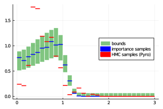
Figure 2. Histogram of samples from two inference algorithms (importance sampling and Pyro’s HMC), and the guaranteed bounds from Beutner et al. (2022). The bounds show that Pyro’s HMC produces wrong results. (Source: Beutner et al. (2022))

Checking approximate inference

In the context of Bayesian inference, the bounds can be useful to check and debug approximate inference algorithms and their implementations. If the approximate results clearly contradict the bounds, the inference algorithm is likely incorrect, or some of its assumptions are violated, or it has not converged. Beutner et al. (2022) provide an example of this: the inference tool Pyro yields wrong results for a probabilistic program with loops, but their bounds can detect this issue (Fig. 2). Another problem with approximate inference is the tail behavior of the posterior distribution, which is often crucial for the quality of the approximation (Liang et al., 2023). Previous work on guaranteed bounds (Beutner et al., 2022; Wang et al., 2024) does not address this aspect, but our work can bound the tail behavior as well.

Table 1. Comparison of our two approaches with the most relevant related work on probabilistic programs with loops. (Cond.: supports (Bayesian) conditioning; Inf.: branching on variables with infinite support is allowed; Cont.: continuous distributions allowed; Auto.: fully automated; Prob.: computes/bounds probabilities; Mom.: computes/bounds moments; Tails: computes/bounds tail asymptotics of this shape. Partial support is denoted by “$\sim$”.)

	Type	Cond.?	Inf.?	Cont.?	Auto.?	Prob.?	Mom.?	Tails?
Moosbrugger et al. (2022)	exact	✗	✗	✓	✓	$\sim$	✓	$O(n^{-k})$
Beutner et al. (2022)	bounds	✓	✓	✓	✓	✓	✗	✗
Wang et al. (2024)	bounds	✓	✓	✓	✓	✓	✗	✗
Klinkenberg et al. (2024)	exact	✓	✓	✗	✗	✓	✓	✗
Resid. mass sem. (Section 3)	bounds	✓	✓	✗	✓	✓	✗	✗
Geom. bounds (Section 4)	bounds	✓	✓	✗	✓	✓	✓	$O(c^{n})$

Problem Statement

Given a probabilistic program with posterior distribution $\mu$ on $\mathbb{N}$, our goal is to bound:

1. probability masses: given $n\in\mathbb{N}$, find $l\mathchar 44\relax\nolinebreak[3]u\in[0\mathchar 44\relax\nolinebreak[3]1]$ such that $l\leq\mathbb{P}_{X\sim\mu}[X=n]\leq u$;

2. moments: given $k\in\mathbb{N}$, find $l\mathchar 44\relax\nolinebreak[3]u\in\mathbb{\mathbb{R}}_{\geq 0}$ such that $l\leq\mathbb{E}_{X\sim\mu}[X^{k}]\leq u$;

3. tail asymptotics: find $c\in[0\mathchar 44\relax\nolinebreak[3]1)$ such that $\mathbb{P}_{X\sim\mu}[X=n]=O(c^{n})$.

1.3. Contributions

In this paper, we develop two new methods to compute guaranteed bounds on the distribution of discrete probabilistic programs with loops and conditioning. Lower bounds can simply be found by unrolling each loop a finite number of times. The main challenge is upper bounds and we attack it in two ways: the first is simple, always applicable, and efficient, but coarse; the second is more sophisticated and expensive, but yields much more informative bounds if applicable. A summary of the most relevant related work is presented in Table 1 and a detailed account in Section 7.

The first semantics, called residual mass semantics (Section 3), is based on the simple idea of bounding the remaining probability mass after the loop unrollings, which has not previously been described, to our knowledge. We make the following contributions:

• We introduce the residual mass as a simple but effective idea to bound posterior probabilities.

• We prove soundness and convergence of the bounds to the true distribution (as loops are unrolled further and further).

• We implement the semantics in a tool called Diabolo and demonstrate empirically that the implementation is more efficient than previous systems (Section 6.3).

The second semantics, called geometric bound semantics (Section 4), is the main novelty of this paper. The idea is to bound the distribution of loops in a more fine-grained manner with geometric tails, rather than a flat bound as in the first semantics.

• We present the concept of a contraction invariant for a loop, which yields upper bounds on the distribution (Section 4.1).

• We introduce a family of distributions called eventually geometric distributions (EGDs) that are used as an abstract domain to overapproximate the distribution of a loop (Section 4.2).

• We present the geometric bound semantics (Section 4.3) which reduces the synthesis problem of such an invariant to solving a system of polynomial inequalities. If successful, it immediately yields bounds on probability masses and, contrary to the first semantics, also on moments and tail probabilities of the program distribution.

• We prove soundness of the semantics and convergence of the bounds, as loops are unrolled further and further (Section 4.5).

• We identify necessary conditions and sufficient conditions for its applicability (Section 4.5).

• We fully automate it in our tool Diabolo (Section 5): contrary to previous work (Klinkenberg et al., 2024), it does not rely on the user to provide a loop invariant (template).

• We demonstrate its applicability on a large proportion of benchmarks from the literature and compare it to previous approaches and the residual mass semantics (Section 6).

Full proofs and additional details can be found in Appendices A, B, C and D and Zaiser (2024b).

1.4. Limitations

Our work deals with discrete probabilistic programs with hard conditioning. This means that programs cannot sample or observe from continuous distributions. Variables in our programming language take values in $\mathbb{N}$; negative numbers are not supported (see Section 8.1 for possible extensions). While our language is Turing-complete, some arithmetic operations like multiplication as well as some common infinite-support distributions (e.g. Poisson) are not directly supported (see Section 2.2 for details on our language’s expressivity). The initial values of the program variables are fixed: our methods cannot reason parametrically about these inputs.

The residual mass semantics can yield bounds on the distribution of any such probabilistic program, but convergence with increasing unrolling is only guaranteed if the program terminates almost surely. If the program distribution has infinite support, we cannot bound the moments or tails: the bound does not contain enough information for this.

The geometric bound semantics yields EGD bounds, which allow bounding moments and tails. On the other hand, such bounds do not exist for all programs. Our experiments show that this is not a big concern for many probabilistic programs with loops in practice: EGD bounds exist for a majority of examples we found in the literature. Another limitation of EGD bounds is that they cannot represent correlation of the tails of two variables, which may lead to imprecise tail bounds or failing to find bounds at all. Finally, solving the system of polynomial inequalities arising from the semantics, while decidable, can be hard in practice and does not scale to very large programs. It should be noted that scalability is a general issue in probabilistic program analysis owing to the hardness of the problem (Dagum and Luby, 1993) and not specific to our work.

1.5. Notation and conventions

We use the Iverson brackets $[\varphi]$ to mean 1 if $\varphi$ is satisfied and 0 otherwise. We write variables representing vectors in bold (${\bm{\alpha}}$), tensors (multidimensional arrays) in uppercase and bold ($\mathbf{T}$), and random or program variables in uppercase ($X$). We write $\mathbf{0}$ and $\mathbf{1}$ for the constant zero and one functions. We write $\mathbf{0}_{n}$ and $\mathbf{1}_{n}$ for the zero and one vectors in $\mathbb{R}^{n}$. To update the $k$-th component of a vector ${\bm{\alpha}}$, we write ${\bm{\alpha}}[k\mapsto v]$. Vectors ${\bm{\alpha}}\in\mathbb{R}^{n}$ are indexed as $\alpha_{1}\mathchar 44\relax\nolinebreak[3]\dots\mathchar 44\relax\nolinebreak[3]\alpha_{n}$. We abbreviate $[d]:=\{0\mathchar 44\relax\nolinebreak[3]\dots\mathchar 44\relax\nolinebreak[3]d-1\}$. Tensors $\mathbf{T}\in\mathbb{R}^{[d_{1}]\times\dots\times[d_{n}]}$ are indexed as $\mathbf{T}_{i_{1}\mathchar 44\relax\nolinebreak[3]\dots\mathchar 44\relax\nolinebreak[3]i_{n}}$ where $i_{k}$ ranges from $0$ to $d_{k}-1$. We write $\mathbf{0}_{[d_{1}]\times\dots\times[d_{n}]}$ or simply $\mathbf{0}$ for the zero tensor in $\mathbb{R}^{[d_{1}]\times\dots\times[d_{n}]}$. We write $|\mathbf{T}|=(d_{1}\dots\mathchar 44\relax\nolinebreak[3]d_{n})$ for the dimensions of $\mathbf{T}\in\mathbb{R}^{[d_{1}]\times\dots\times[d_{n}]}$, and in particular $|\mathbf{T}|_{i}=d_{i}$. To index $\mathbf{T}$ along dimension $k$, we write $\mathbf{T}_{k:j}\in\mathbb{R}^{[d_{1}]\times\cdots\times[d_{k-1}]\times[d_{k+1}]\times\cdots\times[d_{n}]}$, which is defined by $(\mathbf{T}_{k:j})_{i_{1}\mathchar 44\relax\nolinebreak[3]\dots\mathchar 44\relax\nolinebreak[3]i_{k-1}\mathchar 44\relax\nolinebreak[3]i_{k+1}\mathchar 44\relax\nolinebreak[3]\dots\mathchar 44\relax\nolinebreak[3]i_{n}}=\mathbf{T}_{i_{1}\mathchar 44\relax\nolinebreak[3]\dots\mathchar 44\relax\nolinebreak[3]i_{k-1}\mathchar 44\relax\nolinebreak[3]j\mathchar 44\relax\nolinebreak[3]i_{k+1}\mathchar 44\relax\nolinebreak[3]\dots\mathchar 44\relax\nolinebreak[3]i_{n}}$. We often write tensor indices as ${\bm{i}}:=(i_{1}\mathchar 44\relax\nolinebreak[3]\dots\mathchar 44\relax\nolinebreak[3]i_{n})$ for brevity. We also abbreviate ${\bm{\alpha}}^{{\bm{i}}}:=\prod_{k=1}^{n}\alpha_{i}^{i_{k}}$. Other binary operations ($+$, $-$, $\min$, $\max$, etc.) work elementwise on vectors and tensors, e.g. $({\bm{\alpha}}+{\bm{\beta}})_{j}:=\alpha_{j}+\beta_{j}$ and ${\bm{\alpha}}\leq{\bm{\beta}}$ if and only if $\alpha_{j}\leq\beta_{j}$ for all $j$.

2. Background

2.1. Probability and measure theory

All probability spaces $M$ in this work are equipped with the discrete $\sigma$-algebra $\mathcal{P}(M)$. The set of measures on a space $M$ is denoted by $\operatorname{Meas}(M)$. The restriction of a measure $\mu\in\operatorname{Meas}(M)$ to a set $M^{\prime}\subseteq M$ is denoted by $\mu|_{M^{\prime}}$. The mass function $m:M\to[0\mathchar 44\relax\nolinebreak[3]1]$ of a measure $\mu\in\operatorname{Meas}(M)$ is defined by $m(x):=\mu(\{x\})$. By abuse of notation, we will usually write $\mu$ for $m$ as well. We will use the words distribution and measure interchangeably, but a probability distribution is a measure $\mu$ with total mass $\mu(M)=1$. The $k$-th moment of a distribution $\mu\in\operatorname{Meas}(\mathbb{N})$ is defined as $\mathbb{E}_{X\sim\mu}[X^{k}]:=\sum_{x\in\mathbb{N}}\mu(x)\cdot x^{k}$. The tail of a distribution refers to the region far away from the mean. A distribution $\mu$ on $\mathbb{N}$ has tail asymptotics $f(n)$ if $\mu(n)=\Theta(f(n))$. The ${\color[rgb]{0,.5,.5}\mathsf{Dirac}}(x)$ distribution has the mass function ${\color[rgb]{0,.5,.5}\mathsf{Dirac}}(x)(y)=[x=y]$; the ${\color[rgb]{0,.5,.5}\mathsf{Bernoulli}}(\rho)$ distribution for $\rho\in[0\mathchar 44\relax\nolinebreak[3]1]$ is given by ${\color[rgb]{0,.5,.5}\mathsf{Bernoulli}}(\rho)(0)=1-\rho$ and ${\color[rgb]{0,.5,.5}\mathsf{Bernoulli}}(\rho)(1)=\rho$; the ${\color[rgb]{0,.5,.5}\mathsf{Uniform}}\{a\mathchar 44\relax\nolinebreak[3]\dots\mathchar 44\relax\nolinebreak[3]b\}$ distribution for $a<b\in\mathbb{N}$ by ${\color[rgb]{0,.5,.5}\mathsf{Uniform}}\{a\mathchar 44\relax\nolinebreak[3]\dots\mathchar 44\relax\nolinebreak[3]b\}(n)=\frac{[a\leq n\leq b]}{b-a+1}$; and the ${\color[rgb]{0,.5,.5}\mathsf{Geometric}}(\rho)$ distribution for $\rho\in(0\mathchar 44\relax\nolinebreak[3]1]$ by ${\color[rgb]{0,.5,.5}\mathsf{Geometric}}(\rho)(n)=(1-\rho)^{n}\cdot\rho$.

2.2. Probabilistic programming language

Our programming language is a simple imperative language with a fixed number of variables ${\bm{X}}=(X_{1}\mathchar 44\relax\nolinebreak[3]\dots\mathchar 44\relax\nolinebreak[3]X_{n})$. Each variable only takes values in $\mathbb{N}$. We consider the following minimal programming language where $P$ denotes programs and $E$ denotes events.

$$P ::={\color[rgb]{.5,0,.5}\mathsf{skip}}\mid P_{1};P_{2}\mid X_{k}:=0\mid X_{k}\mathbin{{+}{=}}a\mid X_{k}\mathbin{{\dot{-}}{=}}1\mid{\color[rgb]{.5,0,.5}\mathsf{if}}\,{E}\,\allowbreak\{P_{1}\}\,\allowbreak{\color[rgb]{.5,0,.5}\mathsf{else}}\,\{P_{2}\}\mid{\color[rgb]{.5,0,.5}\mathsf{while}}\,{E}\,\allowbreak\{P_{1}\}\mid{\color[rgb]{.5,0,.5}\mathsf{fail}}$$

$$E ::=X_{k}=a\mid{\color[rgb]{.5,0,.5}\mathsf{flip}}(\rho)\mid\lnot E_{1}\mid E_{1}\land E_{2}$$

where $a\in\mathbb{N}\mathchar 44\relax\nolinebreak[3]\rho\in[0\mathchar 44\relax\nolinebreak[3]1]$ are literals. We explain the constructs briefly: ${\color[rgb]{.5,0,.5}\mathsf{skip}}$ does nothing; $P_{1};P_{2}$ executes $P_{1}$ and then $P_{2}$; $X_{k}:=0$ sets $X_{k}$ to 0; $X_{k}\mathbin{{+}{=}}a$ increments $X_{k}$ by $a$; $X_{k}\mathbin{{\dot{-}}{=}}1$ decrements $X_{k}$ by 1 but clamped at 0 ($X_{k}:=\max(X_{k}-1\mathchar 44\relax\nolinebreak[3]0)$); ${\color[rgb]{.5,0,.5}\mathsf{if}}\,{E}\,\allowbreak\{P_{1}\}\,\allowbreak{\color[rgb]{.5,0,.5}\mathsf{else}}\,\{P_{2}\}$ executes $P_{1}$ if the event $E$ occurs and $P_{2}$ otherwise; ${\color[rgb]{.5,0,.5}\mathsf{while}}\,{E}\,\allowbreak\{P_{1}\}$ repeats $P_{1}$ as long as $E$ occurs; ${\color[rgb]{.5,0,.5}\mathsf{fail}}$ states a contradictory observation, i.e. ${\color[rgb]{.5,0,.5}\mathsf{observe}}\,{\color[rgb]{.5,0,.5}\mathsf{false}}$. The ${\color[rgb]{.5,0,.5}\mathsf{flip}}(\rho)$ event occurs with probability $\rho$, like a coin flip with bias $\rho$ coming up heads, or more formally, sampling 1 from an independent ${\color[rgb]{0,.5,.5}\mathsf{Bernoulli}}(\rho)$ distribution. The logical operators $\lnot\mathchar 44\relax\nolinebreak[3]\land$ denote the complement and intersection of events. We usually assume that all variables are set to zero with probability 1 at the beginning.

Syntactic sugar

The language is kept minimal to simplify the presentation. The following syntactic sugar for events (on the left) and statements (on the right) will be convenient:

$$\begin{aligned} E_{1}\lor E_{2}&\;\leadsto\;\lnot(\lnot E_{1}\land\lnot E_{2})\\ X_{k}\in\{a_{1}\mathchar 44\relax\nolinebreak[3]\dots\mathchar 44\relax\nolinebreak[3]a_{m}\}&\;\leadsto\;X_{k}=a_{1}\lor\dots\lor X_{k}=a_{m}\\ X_{k}<a&\;\leadsto\;X_{k}\in\{0\mathchar 44\relax\nolinebreak[3]\dots\mathchar 44\relax\nolinebreak[3]a-1\}\\ X_{k}\leq a&\;\leadsto\;X_{k}<a+1\\ X_{k}\geq a&\;\leadsto\;\lnot(X_{k}<a)\\ X_{k}>a&\;\leadsto\;\lnot(X_{k}\leq a)\end{aligned}\;\begin{aligned} X_{k}:=c&\;\leadsto\;X_{k}:=0;X_{k}\mathbin{{+}{=}}c\\ \{P_{1}\}\mathrel{[\rho]}\{P_{2}\}&\;\leadsto\;{\color[rgb]{.5,0,.5}\mathsf{if}}\,{{\color[rgb]{.5,0,.5}\mathsf{flip}}(\rho)}\,\allowbreak\{P_{1}\}\,\allowbreak{\color[rgb]{.5,0,.5}\mathsf{else}}\,\{P_{2}\}\\ X_{k}\sim{\color[rgb]{0,.5,.5}\mathsf{Bernoulli}}(\rho)&\;\leadsto\;\{X_{k}:=1\}\mathrel{[\rho]}\{X_{k}:=0\}\\ {\color[rgb]{.5,0,.5}\mathsf{observe}}\,E&\;\leadsto\;{\color[rgb]{.5,0,.5}\mathsf{if}}\,{E}\,\allowbreak\{{\color[rgb]{.5,0,.5}\mathsf{skip}}\}\,\allowbreak{\color[rgb]{.5,0,.5}\mathsf{else}}\,\{{\color[rgb]{.5,0,.5}\mathsf{fail}}\}\end{aligned}$$

Sampling

The above language does not include a sampling construct, but sampling from the following distributions can be encoded easily: all finite discrete distributions (e.g. Bernoulli, Binomial, Uniform, Categorical), the Geometric and Negative Binomial distributions, as well as shifted versions thereof. Finite discrete distributions can be expressed with branching and the ${\color[rgb]{.5,0,.5}\mathsf{flip}}(\rho)$ event, similarly to ${\color[rgb]{0,.5,.5}\mathsf{Bernoulli}}(\rho)$ shown above. The sampling construct $X_{k}\sim{\color[rgb]{0,.5,.5}\mathsf{Geometric}}(\rho)$ can be expressed as $X_{k}:=0;{\color[rgb]{.5,0,.5}\mathsf{while}}\,{\lnot{\color[rgb]{.5,0,.5}\mathsf{flip}}(\rho)}\,\allowbreak\{X_{k}\mathbin{{+}{=}}1\}$. A negative binomial distribution can be expressed similarly, as a sum of i.i.d. geometrically distributed variables. Sampling from other distributions, such as the Poisson distribution, can also be expressed in principle since our language is Turing-complete, but we are not aware of a simple encoding.

Expressivity

Our language is similar to the cReDiP language in Klinkenberg et al. (2024), but with more restricted sampling. Like cReDiP, our language does not support negative integers, continuous distributions/variables, more complex arithmetic like multiplication, or comparisons of two variables. Note that the non-probabilistic fragment of the language is already Turing-complete because it can simulate a three-counter machine. Thus these missing constructs could be encoded in principle, at the expense of program complexity.

2.3. Standard semantics

The semantics of programs takes an input measure on the state space and yields an output measure. For probabilistic programs without conditioning, the state space of programs would be $\mathbb{N}^{n}$ (Klinkenberg et al., 2020; Zaiser et al., 2023). But in the presence of conditioning, we want to track observations failures, so we add a failure state $\lightning$, which signifies a failed observation. If we just represented failures by setting the measure to 0 (as in Zaiser et al. (2023)), we would not be able to distinguish between observation failures and nontermination (see Klinkenberg et al. (2024) for a detailed discussion). So the semantics of programs transforms measures on the state space $\mathbb{N}^{n}_{\lightning}:=\mathbb{N}^{n}\cup\{\lightning\}$. The intuitive idea is that when actually running a probabilistic program, ${\color[rgb]{.5,0,.5}\mathsf{fail}}$ moves to the failure state $\lightning$ and aborts the program.

Orders on measures and transformers

To define the semantics, we first need to define partial orders on measures and measure transformers, both of which are standard (Kozen, 1981). Given two measures $\mu\mathchar 44\relax\nolinebreak[3]\nu$ on $M$, we say that $\mu\preceq\nu$ if and only if $\mu(S)\leq\nu(S)$ for all sets $S\subseteq M$. On measure transformers $\varphi\mathchar 44\relax\nolinebreak[3]\psi:\operatorname{Meas}(M)\to\operatorname{Meas}(M)$, we define the pointwise lifting of this order: $\varphi\sqsubseteq\psi$ if and only if $\varphi(\mu)\preceq\psi(\mu)$ for all $\mu\in\operatorname{Meas}(M)$. Both orders are $\omega$-complete partial orders.

$$\mu|_{X_{k}=a}(S) :=\mu(\{{\bm{x}}\in S\mid x_{k}=a\})$$

$$\mu|_{{\color[rgb]{.5,0,.5}\mathsf{flip}}(\rho)} :=\rho\cdot\mu|_{\mathbb{N}^{n}}$$

$$\mu|_{\lnot E_{1}} :=\mu|_{\mathbb{N}^{n}}-\mu|_{E_{1}}$$

$$\mu|_{E_{1}\land E_{2}} :=(\mu|_{E_{1}})|_{E_{2}}$$

(a) Standard semantics of events.

$$\llbracket{\color[rgb]{.5,0,.5}\mathsf{skip}}\rrbracket_{\lightning}(\mu) =\mu$$

$$\llbracket P_{1};P_{2}\rrbracket_{\lightning}(\mu) =\llbracket P_{2}\rrbracket_{\lightning}(\llbracket P_{1}\rrbracket_{\lightning}(\mu))$$

$$\llbracket X_{k}:=0\rrbracket_{\lightning}(\mu)(S) =\mu|_{\lightning}(S)+\mu(\{{\bm{x}}\in\mathbb{N}^{n}\mid{\bm{x}}[k\mapsto 0]\in S\})$$

$$\llbracket X_{k}\mathbin{{+}{=}}a\rrbracket_{\lightning}(\mu)(S) =\mu|_{\lightning}(S)+\mu(\{{\bm{x}}\in\mathbb{N}^{n}\mid{\bm{x}}[k\mapsto Y_{k}+a]\in S\})$$

$$\llbracket X_{k}\mathbin{{\dot{-}}{=}}1\rrbracket_{\lightning}(\mu)(S) =\mu|_{\lightning}(S)+\mu(\{{\bm{x}}\in\mathbb{N}^{n}\mid{\bm{x}}[k\mapsto Y_{k}\mathbin{\dot{-}}1]\in S\})$$

$$\llbracket{\color[rgb]{.5,0,.5}\mathsf{if}}\,{E}\,\allowbreak\{P_{1}\}\,\allowbreak{\color[rgb]{.5,0,.5}\mathsf{else}}\,\{P_{2}\}\rrbracket_{\lightning}(\mu) =\mu|_{\lightning}+\llbracket P_{1}\rrbracket_{\lightning}(\mu|_{E})+\llbracket P_{2}\rrbracket_{\lightning}(\mu|_{\lnot E})$$

$$\llbracket{\color[rgb]{.5,0,.5}\mathsf{fail}}\rrbracket_{\lightning}(\mu) =\mu(\mathbb{N}^{n}_{\lightning})\cdot{\color[rgb]{0,.5,.5}\mathsf{Dirac}}(\lightning)$$

$$\llbracket{\color[rgb]{.5,0,.5}\mathsf{while}}\,{E}\,\allowbreak\{P_{1}\}\rrbracket_{\lightning} =\mathsf{lfp}(\Phi_{E\mathchar 44\relax\nolinebreak[3]P_{1}})$$

(b) Standard semantics of statements.

Figure 3. Standard semantics for probabilistic programs.

Semantics

The standard semantics is a straightforward adaption of Kozen (1981); Klinkenberg et al. (2024). For events $E$, it describes how a measure $\mu$ on program states is “restricted” to $E$ (Fig. 3(a)), suggestively written $\mu|_{E}$ like the restriction of $\mu$ to a subset of $\mathbb{N}^{n}_{\lightning}$, even though some events (e.g. ${\color[rgb]{.5,0,.5}\mathsf{flip}}(\rho)$) do not correspond to such a subset. For programs $P$, the statement semantics $\llbracket P\rrbracket_{\lightning}:\operatorname{Meas}(\mathbb{N}^{n}_{\lightning})\to\operatorname{Meas}(\mathbb{N}^{n}_{\lightning})$ describes how $P$ transforms the measure on program states (Fig. 3(b)).

Regarding notation, we write $\mu|_{\lightning}$ for $\mu|_{\{\lightning\}}$, i.e. the restriction of $\mu$ to the failure state $\lightning$, and conversely $\mu|_{\mathbb{N}^{n}}$ for the restriction of $\mu$ to $\mathbb{N}^{n}$, excluding the failure state $\lightning$. In Section 4, we will largely ignore the failure state $\lightning$ and work with distributions on $\mathbb{N}^{n}$. For this purpose, we introduce the simplified standard semantics $\llbracket P\rrbracket:\operatorname{Meas}(\mathbb{N}^{n})\to\operatorname{Meas}(\mathbb{N}^{n})$ defined as $\llbracket P\rrbracket(\mu):=\llbracket P\rrbracket_{\lightning}(\mu)|_{\mathbb{N}^{n}}$. An interesting case is the loop construct, whose semantics is ${\llbracket{\color[rgb]{.5,0,.5}\mathsf{while}}\,{E}\,\allowbreak\{P_{1}\}\rrbracket_{\lightning}}:=\mathsf{lfp}(\Phi_{E\mathchar 44\relax\nolinebreak[3]P_{1}})$ where

$$\Phi_{E\mathchar 44\relax\nolinebreak[3]P_{1}}:(\operatorname{Meas}(\mathbb{N}^{n}_{\lightning})\to\operatorname{Meas}(\mathbb{N}^{n}_{\lightning}))\to(\operatorname{Meas}(\mathbb{N}^{n}_{\lightning})\to\operatorname{Meas}(\mathbb{N}^{n}_{\lightning}))$$

$$\Phi_{E\mathchar 44\relax\nolinebreak[3]P_{1}}(\psi)(\mu):=\mu|_{\lightning}+\mu|_{\lnot E}+\psi(\llbracket P_{1}\rrbracket_{\lightning}(\mu|_{E}))$$

is the unrolling operator and $\mathsf{lfp}(\Phi_{E\mathchar 44\relax\nolinebreak[3]P_{1}})$ denotes its least fixed point with respect to $\sqsubseteq$. Another way to look at it is that $W:=\llbracket{\color[rgb]{.5,0,.5}\mathsf{while}}\,{E}\,\allowbreak\{P_{1}\}\rrbracket_{\lightning}$ is the least fixed point of the unrolling:

$$W(\mu)=\mu|_{\lightning}+\mu|_{\lnot E}+W(\llbracket P_{1}\rrbracket_{\lightning}(\mu|_{E}))\quad\forall\mu\in\operatorname{Meas}(\mathbb{N}^{n}_{\lightning})$$

Conditioning

The ${\color[rgb]{.5,0,.5}\mathsf{fail}}$ construct moves all the mass to the failure state $\lightning$. Recall that the initial distribution of a program is all zeros with probability 1, i.e. ${\color[rgb]{0,.5,.5}\mathsf{Dirac}}(\mathbf{0}_{n})$. Over the course of the program, some of the mass gets lost due to nontermination and some moves to the failure state due to failed observations. Ultimately, we are interested in the distribution conditioned on the observations. These conditional probabilities of ${\bm{X}}={\bm{x}}\in\mathbb{N}^{n}$ are defined as: $\mathbb{P}[{\bm{X}}={\bm{x}}\mid{\bm{X}}\neq\lightning]=\frac{\mathbb{P}[{\bm{X}}={\bm{x}}\land{\bm{X}}\neq\lightning]}{\mathbb{P}[{\bm{X}}\neq\lightning]}=\frac{\mathbb{P}[{\bm{X}}={\bm{x}}]}{1-\mathbb{P}[X=\lightning]}$. Thus we have to remove the mass on $\lightning$ from the subprobability measure $\mu$ of the program and normalize it, which is achieved by the function $\operatorname{normalize}$ turning subprobability measures on $\mathbb{N}^{n}_{\lightning}$ into subprobability measures on $\mathbb{N}^{n}$: $\operatorname{normalize}(\mu):=\frac{\mu-\mu|_{\lightning}}{1-\mu(\lightning)}$. Thus the posterior probability distribution of a program $P$ with initial distribution $\mu$ (usually ${\color[rgb]{0,.5,.5}\mathsf{Dirac}}(\mathbf{0}_{n})$) is given by $\operatorname{normalize}(\llbracket P\rrbracket_{\lightning}(\mu))$. Operationally, we can think of normalization as a rejection sampler of the posterior distribution: it runs the program repeatedly, rejects all runs that end in $\lightning$, and only yields the results of the remaining runs as samples.

Nontermination

Due to the possibility of nontermination, even the normalized measure of a program may not be a probability distribution, only a subprobability distribution (see the discussion in Klinkenberg et al. (2024, Section 3.4)). For example, the loop ${\color[rgb]{.5,0,.5}\mathsf{while}}\,{{\color[rgb]{.5,0,.5}\mathsf{flip}}(1)}\,\allowbreak\{{\color[rgb]{.5,0,.5}\mathsf{skip}}\}$ will never terminate, so both its unnormalized and normalized semantics are always the zero measure. This is not a problem in practice because nontermination is usually considered a bug for statistical models. Tracking observation failures is useful for defining termination, however.

Definition 2.1.

A program $P$ is almost surely terminating on a finite measure $\mu\in\operatorname{Meas}(\mathbb{N}^{n}_{\lightning})$ if $\llbracket P\rrbracket_{\lightning}(\mu)(\mathbb{N}^{n}_{\lightning})=\mu(\mathbb{N}^{n}_{\lightning})$.

The semantics of a program $\llbracket P\rrbracket_{\lightning}$ satisfies the usual properties listed below. The proof is analogous to Klinkenberg et al. (2024).

Lemma 2.2.

For any program $P$, the transformation $\llbracket P\rrbracket_{\lightning}$ is linear and $\omega$-continuous, so in particular monotonic. It also has the property that the total measure does not increase: $\llbracket P\rrbracket_{\lightning}(\mu)(\mathbb{N}^{n}_{\lightning})\leq\mu(\mathbb{N}^{n}_{\lightning})$ for all $\mu\in\operatorname{Meas}(\mathbb{N}^{n}_{\lightning})$.

3. Residual mass semantics

In this section, we first present the lower bounds semantics based on loop unrolling. Since even upper bounds on the normalized posterior require lower bounds on the normalizing constant, these lower bounds are also used as part of our methods for upper bounds. The residual mass semantics extends the lower bound semantics to obtain upper bounds on the unnormalized distribution as well and can thus derive both lower and upper bounds on the normalized posterior. This way, any exact inference method for the loop-free fragment can be transformed into a method to bound the distribution of programs with loops. We present both semantics formally and prove soundness and convergence. Full proofs are given in Appendix A.

3.1. Lower bounds via unrolling

Lower bounds can be computed by unrolling the loop a finite number of times and discarding the part of the distribution that has not exited the loop after the unrollings. Define the $u$-fold unrolling $P^{(u)}$ of a program $P$ by unrolling each loop $u$ times:

$$(P_{1};P_{2})^{(u)} :=P_{1}^{(u)};P_{2}^{(u)}$$

$$({\color[rgb]{.5,0,.5}\mathsf{if}}\,{E}\,\allowbreak\{P_{1}\}\,\allowbreak{\color[rgb]{.5,0,.5}\mathsf{else}}\,\{P_{2}\})^{(u)} :={\color[rgb]{.5,0,.5}\mathsf{if}}\,{E}\,\allowbreak\{P_{1}^{(u)}\}\,\allowbreak{\color[rgb]{.5,0,.5}\mathsf{else}}\,\{P_{2}^{(u)}\}$$

$$({\color[rgb]{.5,0,.5}\mathsf{while}}\,{E}\,\allowbreak\{P\})^{(u)} :=({\color[rgb]{.5,0,.5}\mathsf{while}}\,{E}\,\allowbreak\{P\})_{0}^{(u)}$$

$$({\color[rgb]{.5,0,.5}\mathsf{while}}\,{E}\,\allowbreak\{P\})_{v}^{(u)} :={\color[rgb]{.5,0,.5}\mathsf{if}}\,{E}\,\allowbreak\{P^{(u)};({\color[rgb]{.5,0,.5}\mathsf{while}}\,{E}\,\allowbreak\{P\})_{v+1}^{(u)}\}\,\allowbreak{\color[rgb]{.5,0,.5}\mathsf{else}}\,\{{\color[rgb]{.5,0,.5}\mathsf{skip}}\};\quad\text{for }v<u$$

$$({\color[rgb]{.5,0,.5}\mathsf{while}}\,{E}\,\allowbreak\{P\})_{u}^{(u)} :={\color[rgb]{.5,0,.5}\mathsf{while}}\,{E}\,\allowbreak\{P^{(u)}\}$$

$$P^{(u)} :=P\quad\text{otherwise}$$

Lemma 3.1.

Unrolling does not change the semantics: $\llbracket P\rrbracket_{\lightning}=\llbracket P^{(u)}\rrbracket_{\lightning}$ for all programs $P$ and $u\in\mathbb{N}$.

The lower bound semantics $\llbracket P\rrbracket_{\mathsf{lo}}$ is then defined just like $\llbracket P\rrbracket_{\lightning}$ except that $\llbracket{\color[rgb]{.5,0,.5}\mathsf{while}}\,{E}\,\allowbreak\{P_{1}\}\rrbracket_{\mathsf{lo}}(\mu):=\mathbf{0}$. In other words, $\llbracket P\rrbracket_{\mathsf{lo}}=\llbracket P^{\prime}\rrbracket_{\lightning}$ where $P^{\prime}$ is the program $P$ where all loops are replaced by infinite loops, effectively setting the measure to zero. Its correctness follows from the monotonicity of the standard semantics.

Theorem 3.2 (Soundness of lower bounds).

For all measures $\mu\in\operatorname{Meas}(\mathbb{N}^{n}_{\lightning})$ and programs $P$, we have $\llbracket P\rrbracket_{\mathsf{lo}}(\mu)\preceq\llbracket P\rrbracket_{\lightning}(\mu)$.

The lower bounds will get better as loops are unrolled further and further. In fact, they will converge to the true distribution.

Theorem 3.3 (Convergence of lower bounds).

For all finite measures $\mu\in\operatorname{Meas}(\mathbb{N}^{n}_{\lightning})$ and programs $P$, the lower bound $\llbracket P^{(u)}\rrbracket_{\mathsf{lo}}(\mu)$ converges (in total variation distance) monotonically to the true distribution $\llbracket P\rrbracket_{\lightning}(\mu)$ as $u\to\infty$.

Note that the lower bound semantics involves only finite discrete distributions (for our programming language), which can be represented exactly by a finite array of the probability masses. In fact, any exact semantics for the loop-free fragment (e.g. Zaiser et al. (2023)) leads to lower bounds for programs with loops. A related approach by Jansen et al. (2016) combines unrolling with probabilistic model checking to obtain lower bounds on reachability probabilities and expectations.

3.2. Upper bounds via residual mass

Lower bounds are easy because $\mathbf{0}$ is clearly a lower bound that can be used as a starting point for the fixed point iteration. This strategy does not work for upper bounds since there is no such obvious starting point.

Instead, a simple idea is to use the fact that the total mass of the state distribution can only decrease after program execution (Lemma 2.2). In other words, for a program $P$ with initial distribution $\mu\in\operatorname{Meas}(\mathbb{N}^{n}_{\lightning})$, the total mass of the distribution after running $P$ is $\llbracket P\rrbracket_{\lightning}(\mu)(\mathbb{N}^{n}_{\lightning})\leq\mu(\mathbb{N}^{n}_{\lightning})$. So the part of the distribution that we miss in the lower bounds by cutting loops short has a probability mass bounded by the distance to the total mass $\mu(\mathbb{N}^{n}_{\lightning})$ at the start. We call this gap the residual mass of the program $P$ with initial measure $\mu$ and define it as $\llbracket P\rrbracket_{\mathsf{res}}(\mu):=\mu(\mathbb{N}^{n}_{\lightning})-\llbracket P\rrbracket_{\mathsf{lo}}(\mu)(\mathbb{N}^{n}_{\lightning})\in\mathbb{\mathbb{R}}_{\geq 0}$.

The residual mass semantics uses the residual mass to bound probabilities $\llbracket P\rrbracket_{\lightning}(\mu)(S)$ of the program distribution for a set $S\subseteq\mathbb{N}^{n}_{\lightning}$ by analyzing the gap $\llbracket P\rrbracket_{\lightning}(\mu)(S)-\llbracket P\rrbracket_{\mathsf{lo}}(\mu)(S)$ as follows. The gap is maximized if $S=\mathbb{N}^{n}_{\lightning}$ and thus bounded by $\llbracket P\rrbracket_{\lightning}(\mu)(\mathbb{N}^{n}_{\lightning})-\llbracket P\rrbracket_{\mathsf{lo}}(\mu)(\mathbb{N}^{n}_{\lightning})$. Since $\llbracket P\rrbracket_{\lightning}(\mu)(\mathbb{N}^{n}_{\lightning})\leq\mu(\mathbb{N}^{n}_{\lightning})$ by Lemma 2.2, this gap is always bounded by the residual mass. The residual mass semantics can also bound the normalizing constant $1-\llbracket P\rrbracket_{\lightning}(\mu)(\lightning)$ since $\llbracket P\rrbracket_{\mathsf{lo}}(\mu)(\lightning)\leq\llbracket P\rrbracket_{\lightning}(\mu)(\lightning)\leq\llbracket P\rrbracket_{\mathsf{lo}}(\mu)(\lightning)+\llbracket P\rrbracket_{\mathsf{res}}(\mu)$ where the lower bound follows from Theorem 3.2 and the upper bound from the previous argument. Thus it also yields bounds on the (normalized) posterior probabilities. The above soundness argument is made fully rigorous in the following theorem. We also have a convergence theorem for the residual mass semantics, similar to Theorem 3.3.

Theorem 3.4 (Soundness of the residual mass semantics).

Let $P$ be a program and $\mu\in\operatorname{Meas}(\mathbb{N}^{n}_{\lightning})$. Then for all $S\subseteq\mathbb{N}^{n}_{\lightning}$, we can bound the unnormalized probabilities

$$\llbracket P\rrbracket_{\mathsf{lo}}(\mu)(S)\leq\llbracket P\rrbracket_{\lightning}(\mu)(S)\leq\llbracket P\rrbracket_{\mathsf{lo}}(\mu)(S)+\llbracket P\rrbracket_{\mathsf{res}}(\mu)$$

If $\mu$ is a probability measure and $S\subseteq\mathbb{N}^{n}$, we can bound the posterior probabilities:

$$\frac{\llbracket P\rrbracket_{\mathsf{lo}}(\mu)(S)}{1-\llbracket P\rrbracket_{\mathsf{lo}}(\mu)(\lightning)}\leq\operatorname{normalize}(\llbracket P\rrbracket_{\lightning}(\mu))(S)\leq\frac{\llbracket P\rrbracket_{\mathsf{lo}}(\mu)(S)+\llbracket P\rrbracket_{\mathsf{res}}(\mu)}{1-\llbracket P\rrbracket_{\mathsf{lo}}(\mu)(\lightning)-\llbracket P\rrbracket_{\mathsf{res}}(\mu)}$$

Theorem 3.5 (Convergence of the residual mass semantics).

Let $P$ be a program terminating almost surely on a finite measure $\mu\in\operatorname{Meas}(\mathbb{N}^{n}_{\lightning})$. Then the residual mass $\llbracket P^{(u)}\rrbracket_{\mathsf{res}}(\mu)$ converges monotonically to 0 as $u\to\infty$. In particular, the above bounds on $\operatorname{normalize}(\llbracket P^{(u)}\rrbracket_{\lightning}(\mu))(S)$ converge to the true posterior probability as $u\to\infty$.

Since the residual mass semantics only depends on the lower bounds, it can be implemented using the same representations and techniques as the lower bound semantics. We illustrate the residual mass semantics with an example.

Example 3.6 (Residual mass semantics).

Consider again the “die paradox” program (Examples 1.1 and 1) where the variables are ${\bm{X}}:=(\mathit{Throws}\mathchar 44\relax\nolinebreak[3]\mathit{Die})$. After three unrollings, the lower bound distribution $\mu:=\llbracket P^{(3)}\rrbracket_{\mathsf{lo}}(\mu_{0})$ for the initial distribution $\mu_{0}={\color[rgb]{0,.5,.5}\mathsf{Dirac}}(\mathbf{0})$ is given by

$$\mu(s)=\begin{cases}\frac{1}{2}+\frac{1}{3}\cdot\frac{1}{2}=\frac{2}{3}&\text{if }s=\lightning\\ \frac{1}{6}&\text{if }s=(1\mathchar 44\relax\nolinebreak[3]6)\\ \frac{1}{3}\cdot\frac{1}{6}=\frac{1}{18}&\text{if }s=(2\mathchar 44\relax\nolinebreak[3]6)\\ 0&\text{otherwise}\end{cases}$$

because the failure probability is $\frac{1}{2}$ (for $\mathit{Die}\in\{1\mathchar 44\relax\nolinebreak[3]3\mathchar 44\relax\nolinebreak[3]5\}$) and the second iteration is entered in a state other than $\lightning$ with probability $\frac{1}{3}$ (for $\mathit{Die}\in\{2\mathchar 44\relax\nolinebreak[3]4\}$). The residual mass is given by $\llbracket P^{(3)}\rrbracket_{\mathsf{res}}(\mu_{0})=\mu_{0}(\mathbb{N}^{n}_{\lightning})-\mu(\mathbb{N}^{n}_{\lightning})=1-(\frac{2}{3}+\frac{1}{6}+\frac{1}{18})=\frac{1}{9}$. This yields the following bounds on $\llbracket P\rrbracket_{\lightning}(\mu_{0})(s)$ for $s\in\mathbb{N}^{n}_{\lightning}$:

$$\llbracket P\rrbracket_{\lightning}(\mu_{0})(s)\in\begin{cases}[\frac{2}{3}\mathchar 44\relax\nolinebreak[3]\frac{7}{9}]&\text{if }s=\lightning\\ [\frac{1}{6}\mathchar 44\relax\nolinebreak[3]\frac{5}{18}]&\text{if }s=(1\mathchar 44\relax\nolinebreak[3]6)\\ [\frac{1}{18}\mathchar 44\relax\nolinebreak[3]\frac{1}{6}]&\text{if }s=(2\mathchar 44\relax\nolinebreak[3]6)\\ [0\mathchar 44\relax\nolinebreak[3]\frac{1}{9}]&\text{otherwise}\end{cases}$$

Hence the normalizing constant $1-\llbracket P\rrbracket_{\lightning}(\mu_{0})$ is in $[\frac{2}{9}\mathchar 44\relax\nolinebreak[3]\frac{1}{3}]$, which yields the following normalized bounds. They are not very tight but can be improved by increasing the unrolling depth.

$$\operatorname{normalize}(\llbracket P\rrbracket_{\lightning}(\mu_{0}))(s)\in\begin{cases}[\frac{1}{6}\cdot 3\mathchar 44\relax\nolinebreak[3]\frac{5}{18}\cdot\frac{9}{2}]=[\frac{1}{2}\mathchar 44\relax\nolinebreak[3]\frac{5}{4}]&\text{if }s=(1\mathchar 44\relax\nolinebreak[3]6)\\ [\frac{1}{18}\cdot 3\mathchar 44\relax\nolinebreak[3]\frac{1}{6}\cdot\frac{9}{2}]=[\frac{1}{6}\mathchar 44\relax\nolinebreak[3]\frac{3}{4}]&\text{if }s=(2\mathchar 44\relax\nolinebreak[3]6)\\ [0\mathchar 44\relax\nolinebreak[3]\frac{1}{9}\cdot\frac{9}{2}]=[0\mathchar 44\relax\nolinebreak[3]\frac{1}{2}]&\text{otherwise}\end{cases}$$

4. Geometric bound semantics

A big problem with the residual mass semantics is that we can bound the total measure and individual probabilities, but not moments and tail distributions of distributions with infinite support. This problem cannot be fully resolved in general because moments do not always exist.

Example 4.1.

The moments of the distribution of the following program are infinite:

$$X:=0;Y:=1;$$

$${\color[rgb]{.5,0,.5}\mathsf{while}}\,{{\color[rgb]{.5,0,.5}\mathsf{flip}}(1/2)}\,\allowbreak\{$$

$$\qquad{\color[rgb]{.5,0,.5}\mathsf{while}}\,{Y>0}\,\allowbreak\{X\mathbin{{+}{=}}1;Y\mathbin{{\dot{-}}{=}}1\};$$

$$\qquad{\color[rgb]{.5,0,.5}\mathsf{while}}\,{X>0}\,\allowbreak\{X\mathbin{{\dot{-}}{=}}1;Y\mathbin{{+}{=}}2\};\}$$

The loop body multiplies $Y$ by 2 using the auxiliary variable $X$. This program is almost surely terminating and with result probabilities $\mathbb{P}[X=0\mathchar 44\relax\nolinebreak[3]Y=2^{m}]=2^{-m}$ for $m>0$ and zero elsewhere. Hence the $k$-th moment ($k\geq 1$) of $Y$ is $\mathbb{E}[Y^{k}]=\sum_{m=1}^{\infty}\mathbb{P}[X=0\mathchar 44\relax\nolinebreak[3]Y=2^{m}]\cdot 2^{km}\geq\sum_{m=1}^{\infty}1=\infty$.

However, in many cases, more precise upper bounds can be found that also yield bounds on moments and tails for distributions with infinite support. There are two key ideas that make this geometric bound semantics possible: contraction invariants and eventually geometric distributions (EGDs). Like the residual mass semantics, it builds on the lower bound semantics in order to obtain both lower and upper bounds on the normalized posterior.

4.1. Contraction invariants

If a loop $L={\color[rgb]{.5,0,.5}\mathsf{while}}\,{E}\,\allowbreak\{B\}$ terminates almost surely on an initial distribution $\mu$, all the probability mass that entered the loop must eventually exit the loop. Inspired by this observation, we consider the following assumption:

(1) $$\llbracket B\rrbracket_{\lightning}(\mu|_{E})\preceq c\cdot\mu\text{ with }0\leq c<1$$

In words: the probability distribution at the start of the next loop iteration decreases uniformly by a factor of $c$. This assumption looks very strong and is often violated in practice, but if we assume for a minute that it holds, what can we derive? Recall the fixpoint equation of loops:

$$\llbracket{\color[rgb]{.5,0,.5}\mathsf{while}}\,{E}\,\allowbreak\{B\}\rrbracket_{\lightning}(\mu) =\mu|_{\lightning}+\mu|_{\lnot E}+\llbracket{\color[rgb]{.5,0,.5}\mathsf{while}}\,{E}\,\allowbreak\{B\}\rrbracket_{\lightning}(\llbracket B\rrbracket_{\lightning}(\mu|_{E}))$$

$$\preceq\mu|_{\lightning}+\mu|_{\lnot E}+c\cdot\llbracket{\color[rgb]{.5,0,.5}\mathsf{while}}\,{E}\,\allowbreak\{B\}\rrbracket_{\lightning}(\mu)$$ by Eq. 1 and linearity

By rearranging, we find the upper bound $\llbracket{\color[rgb]{.5,0,.5}\mathsf{while}}\,{E}\,\allowbreak\{B\}\rrbracket_{\lightning}(\mu)\preceq\frac{\mu|_{\lightning}+\mu|_{\lnot E}}{1-c}$.

Unfortunately, the initial distribution $\mu$ will usually not satisfy Eq. 1 directly. But we may be able to increase $\mu$ to $\nu\succeq\mu$ such that $\nu$ satisfies $\llbracket B\rrbracket_{\lightning}(\nu|_{E})\preceq c\cdot\nu$ with $0\leq c<1$. We then call $\nu$ a contraction invariant or $c$-contraction invariant of $\mu$. Surprisingly, such a contraction invariant $\nu$ can often be found in practice (see Section 6.1), and we can then derive the following upper bound on the distribution after the loop: $\llbracket{\color[rgb]{.5,0,.5}\mathsf{while}}\,{E}\,\allowbreak\{B\}\rrbracket_{\lightning}(\mu)\preceq\llbracket{\color[rgb]{.5,0,.5}\mathsf{while}}\,{E}\,\allowbreak\{B\}\rrbracket_{\lightning}(\nu)\preceq\frac{\nu|_{\lightning}+\nu|_{\lnot E}}{1-c}$.

4.2. Eventually geometric distributions (EGDs)

How can we find such a contraction invariant $\nu$? We clearly have to restrict the candidate set for $\nu$ in some way. Specifically, we consider a class of distributions that generalize geometric distributions. Recall that a ${\color[rgb]{0,.5,.5}\mathsf{Geometric}}(\beta)$ distribution has probability masses $p(i)=\beta(1-\beta)^{i}\propto(1-\beta)^{i}$ with a decay rate of $1-\beta$. For the multivariate setting, we consider products of independent geometric distributions, but with a twist: probabilities of small values are allowed to differ for additional flexibility. This section makes extensive use of vector and tensor notations as described in Section 1.5.

Definition 4.2.

Let $\mathbf{P}\in\mathbb{\mathbb{R}}_{\geq 0}^{[d_{1}+1]\times\cdots\times[d_{n}+1]}$ be an $n$-dimensional tensor and ${\bm{\alpha}}\in[0\mathchar 44\relax\nolinebreak[3]1)^{n}$. The $n$-dimensional eventually geometric distribution (EGD) with initial block $\mathbf{P}$ and decay rates ${\bm{\alpha}}$, written ${\color[rgb]{0,.5,.5}\mathsf{EGD}}\mathopen{}\left(\mathbf{P}\mathchar 44\relax\nolinebreak[3]{\bm{\alpha}}\right)\mathclose{}\in\operatorname{Meas}(\mathbb{N}^{n})$ is defined by the following mass function (for ${\bm{i}}=(i_{1}\mathchar 44\relax\nolinebreak[3]\dots\mathchar 44\relax\nolinebreak[3]i_{n})\in\mathbb{N}^{n}$):

$${\color[rgb]{0,.5,.5}\mathsf{EGD}}\mathopen{}\left(\mathbf{P}\mathchar 44\relax\nolinebreak[3]{\bm{\alpha}}\right)\mathclose{}({\bm{i}})=\mathbf{P}_{\min({\bm{i}}\mathchar 44\relax\nolinebreak[3]|\mathbf{P}|-\mathbf{1}_{n})}\cdot{\bm{\alpha}}^{\max({\bm{i}}-|\mathbf{P}|+\mathbf{1}_{n}\mathchar 44\relax\nolinebreak[3]\mathbf{0}_{n})}=\mathbf{P}_{\min(i_{1}\mathchar 44\relax\nolinebreak[3]d_{1})\mathchar 44\relax\nolinebreak[3]\dots\mathchar 44\relax\nolinebreak[3]\min(i_{n}\mathchar 44\relax\nolinebreak[3]d_{n})}\alpha_{1}^{\max(i_{1}-d_{1}\mathchar 44\relax\nolinebreak[3]0)}\cdots\alpha_{n}^{\max(i_{n}-d_{n}\mathchar 44\relax\nolinebreak[3]0)}.$$

Note that an EGD is not necessarily a probability measure. One can think of ${\color[rgb]{0,.5,.5}\mathsf{EGD}}\mathopen{}\left(\mathbf{P}\mathchar 44\relax\nolinebreak[3]{\bm{\alpha}}\right)\mathclose{}$ as a scaled product of independent ${\color[rgb]{0,.5,.5}\mathsf{Geometric}}(1-\alpha_{i})$ distributions, except it may differ in a finite “prefix” of size $d_{j}$ in each dimension $j$. Outside this initial block, the probability masses are extended like in a geometric distribution with decay rate $\alpha_{j}$ in each dimension $j$. In other words: eventually, for values $i_{j}>d_{j}$, the $j$-th component of ${\color[rgb]{0,.5,.5}\mathsf{EGD}}\mathopen{}\left(\mathbf{P}\mathchar 44\relax\nolinebreak[3]{\bm{\alpha}}\right)\mathclose{}$ behaves like a ${\color[rgb]{0,.5,.5}\mathsf{Geometric}}(1-\alpha_{j})$ distribution; hence the name. They were originally motivated by the shape of their generating function (Zaiser, 2024b, Appendix C.1). EGDs can be seen as a subclass of multivariate discrete phase-type distributions (Campillo Navarro, 2018). (Discrete phase-type distributions (Neuts, 1975) describe the absorption time in a Markov chain with one absorbing state (Bladt and Nielsen, 2017, Section 1.2.6).)

Example 4.3.

Consider the two-dimensional EGD given by ${\color[rgb]{0,.5,.5}\mathsf{EGD}}\mathopen{}\left(\mathbf{P}\mathchar 44\relax\nolinebreak[3](\alpha_{1}\mathchar 44\relax\nolinebreak[3]\alpha_{2})\right)\mathclose{}$ with $\mathbf{P}\in\mathbb{\mathbb{R}}_{\geq 0}^{[2]\times[2]}$, i.e. $\mathbf{P}$ is a matrix $\mathbf{P}=\begin{pmatrix}\mathbf{P}_{0\mathchar 44\relax\nolinebreak[3]0}&\mathbf{P}_{0\mathchar 44\relax\nolinebreak[3]1}\\ \mathbf{P}_{1\mathchar 44\relax\nolinebreak[3]0}&\mathbf{P}_{1\mathchar 44\relax\nolinebreak[3]1}\end{pmatrix}$. Its probability masses are given in the following table:

${\color[rgb]{0,.5,.5}\mathsf{EGD}}\mathopen{}\left(\mathbf{P}\mathchar 44\relax\nolinebreak[3](\alpha_{1}\mathchar 44\relax\nolinebreak[3]\alpha_{2})\right)\mathclose{}(x_{1}\mathchar 44\relax\nolinebreak[3]x_{2})$	$x_{2}=0$	$x_{2}=1$	$x_{2}=2$	…	$x_{2}=j$
$x_{1}=0$	$\mathbf{P}_{0\mathchar 44\relax\nolinebreak[3]0}$	$\mathbf{P}_{0\mathchar 44\relax\nolinebreak[3]1}$	$\mathbf{P}_{0\mathchar 44\relax\nolinebreak[3]1}\cdot\alpha_{2}$	…	$\mathbf{P}_{0\mathchar 44\relax\nolinebreak[3]1}\cdot\alpha_{2}^{j-1}$
$x_{1}=1$	$\mathbf{P}_{1\mathchar 44\relax\nolinebreak[3]0}$	$\mathbf{P}_{1\mathchar 44\relax\nolinebreak[3]1}$	$\mathbf{P}_{1\mathchar 44\relax\nolinebreak[3]1}\cdot\alpha_{2}$	…	$\mathbf{P}_{1\mathchar 44\relax\nolinebreak[3]1}\cdot\alpha_{2}^{j-1}$
$x_{1}=2$	$\mathbf{P}_{1\mathchar 44\relax\nolinebreak[3]0}\cdot\alpha_{1}$	$\mathbf{P}_{1\mathchar 44\relax\nolinebreak[3]1}\cdot\alpha_{1}$	$\mathbf{P}_{1\mathchar 44\relax\nolinebreak[3]1}\cdot\alpha_{1}\alpha_{2}$	…	$\mathbf{P}_{1\mathchar 44\relax\nolinebreak[3]1}\cdot\alpha_{1}\cdot\alpha_{2}^{j-1}$
$\vdots$	$\vdots$	$\vdots$	$\vdots$	$\ddots$	$\vdots$
$x_{1}=i$	$\mathbf{P}_{1\mathchar 44\relax\nolinebreak[3]0}\cdot\alpha_{1}^{i-1}$	$\mathbf{P}_{1\mathchar 44\relax\nolinebreak[3]1}\cdot\alpha_{1}^{i-1}$	$\mathbf{P}_{1\mathchar 44\relax\nolinebreak[3]1}\cdot\alpha_{1}^{i-1}\cdot\alpha_{2}$	…	$\mathbf{P}_{1\mathchar 44\relax\nolinebreak[3]1}\cdot\alpha_{1}^{i-1}\cdot\alpha_{2}^{j-1}$

Here we can see that after the initial block of size $2\times 2$, the probability masses are extended with decay rate $\alpha_{1}$ in the first dimension and $\alpha_{2}$ in the second dimension.

Why did we pick EGDs as the shape of our bounds? There are several reasons.

1. Interpretability: EGDs can easily be understood as geometric distributions, where the probability masses for small values (up to some threshold) have been modified. The relationship with the geometric distribution also makes it easier to compute its moments and the tail asymptotics can be read directly off the parameter ${\bm{\alpha}}$ (see Theorem 4.5 below).

2. Expressiveness: the reason we allow the “start” of the distribution to deviate from geometric distributions is necessary for flexibility. If only exact geometric distributions were allowed, typical program operations like increasing or decreasing a variable (i.e. shifting the geometric distribution) could not be represented precisely enough and the whole approach would fail.

3. Tractability: the order $\preceq$ is easy to check for EGDs, as we will see, because the probability masses follow a simple pattern. In fact, we will see that $\preceq$ for EGDs is equivalent to the satisfiability of a system of polynomial inequalities. If we had based our semantics on an extension of, say, negative binomial distributions (of which geometric distributions are a special case), deciding the order would be harder because binomial coefficients start appearing in the probability masses.

As evidence for interpretability and tractability, we show how to marginalize EGDs and how to compute their moments. This is also needed to extract bounds on the moment from EGD bounds.

Lemma 4.4 (Marginalizing EGDs).

Marginalizing out the $k$-th distribution from ${\color[rgb]{0,.5,.5}\mathsf{EGD}}\mathopen{}\left(\mathbf{P}\mathchar 44\relax\nolinebreak[3]{\bm{\alpha}}\right)\mathclose{}$ yields ${\color[rgb]{0,.5,.5}\mathsf{EGD}}\mathopen{}\left(\mathbf{Q}\mathchar 44\relax\nolinebreak[3]{\bm{\beta}}\right)\mathclose{}$ with ${\bm{\beta}}=(\alpha_{1}\mathchar 44\relax\nolinebreak[3]\dots\mathchar 44\relax\nolinebreak[3]\alpha_{k-1}\mathchar 44\relax\nolinebreak[3]\alpha_{k+1}\mathchar 44\relax\nolinebreak[3]\dots\alpha_{n})$ and $\mathbf{Q}=\sum_{j=0}^{|\mathbf{P}|_{k}-2}\mathbf{P}_{k:j}+\frac{\mathbf{P}_{k:|\mathbf{P}|_{k}-1}}{1-\alpha_{k}}$.

Theorem 4.5 (Moments and tails of EGDs).

Let ${\color[rgb]{0,.5,.5}\mathsf{EGD}}\mathopen{}\left(\mathbf{P}\mathchar 44\relax\nolinebreak[3]\alpha\right)\mathclose{}$ be a one-dimensional EGD with $\mathbf{P}\in\mathbb{\mathbb{R}}_{\geq 0}^{[d+1]}$. Then its tail asymptotics is ${\color[rgb]{0,.5,.5}\mathsf{EGD}}\mathopen{}\left(\mathbf{P}\mathchar 44\relax\nolinebreak[3]\alpha\right)\mathclose{}(n)=O(\alpha^{n})$ and its $k$-th moment is

$$\mathbb{E}_{X\sim{\color[rgb]{0,.5,.5}\mathsf{EGD}}\mathopen{}\left(\mathbf{P}\mathchar 44\relax\nolinebreak[3]\alpha\right)\mathclose{}}[X^{k}]=\sum_{j=0}^{d-1}\mathbf{P}_{j}\cdot j^{k}+\frac{\mathbf{P}_{d}}{1-\alpha}\sum_{i=0}^{k}\binom{k}{i}d^{k-i}\mathbb{E}_{Y\sim{\color[rgb]{0,.5,.5}\mathsf{Geometric}}(1-\alpha)}[Y^{i}]$$

and thus can be computed from the $k$-th moment of a geometric distribution. In particular, the expected value is $\mathbb{E}_{X\sim{\color[rgb]{0,.5,.5}\mathsf{EGD}}\mathopen{}\left(\mathbf{P}\mathchar 44\relax\nolinebreak[3]\alpha\right)\mathclose{}}[X]=\sum_{j=0}^{d-1}\mathbf{P}_{j}\cdot j+\frac{\mathbf{P}_{d}}{1-\alpha}(d+\frac{\alpha}{1-\alpha})$.

Expansion of EGDs

When performing binary operations (e.g. comparison or addition) on EGDs, it will often be convenient to assume that their initial blocks have the same size. In fact, one can always expand the size of the initial block of an EGD without changing the distribution. For example, the distribution from Example 4.3 can equivalently be represented as:

$${\color[rgb]{0,.5,.5}\mathsf{EGD}}\mathopen{}\left(\begin{pmatrix}\mathbf{Q}_{0\mathchar 44\relax\nolinebreak[3]0}&\mathbf{Q}_{0\mathchar 44\relax\nolinebreak[3]1}\\ \mathbf{Q}_{1\mathchar 44\relax\nolinebreak[3]0}&\mathbf{Q}_{1\mathchar 44\relax\nolinebreak[3]1}\end{pmatrix}\mathchar 44\relax\nolinebreak[3]{\bm{\alpha}}\right)\mathclose{} ={\color[rgb]{0,.5,.5}\mathsf{EGD}}\mathopen{}\left(\begin{pmatrix}\mathbf{Q}_{0\mathchar 44\relax\nolinebreak[3]0}&\mathbf{Q}_{0\mathchar 44\relax\nolinebreak[3]1}\\ \mathbf{Q}_{1\mathchar 44\relax\nolinebreak[3]0}&\mathbf{Q}_{1\mathchar 44\relax\nolinebreak[3]1}\\ \mathbf{Q}_{1\mathchar 44\relax\nolinebreak[3]0}\alpha_{1}&\mathbf{Q}_{1\mathchar 44\relax\nolinebreak[3]1}\alpha_{1}\end{pmatrix}\mathchar 44\relax\nolinebreak[3]{\bm{\alpha}}\right)\mathclose{}={\color[rgb]{0,.5,.5}\mathsf{EGD}}\mathopen{}\left(\begin{pmatrix}\mathbf{Q}_{0\mathchar 44\relax\nolinebreak[3]0}&\mathbf{Q}_{0\mathchar 44\relax\nolinebreak[3]1}&\mathbf{Q}_{0\mathchar 44\relax\nolinebreak[3]1}\alpha_{2}&\mathbf{Q}_{0\mathchar 44\relax\nolinebreak[3]1}\alpha_{2}^{2}\\ \mathbf{Q}_{1\mathchar 44\relax\nolinebreak[3]0}&\mathbf{Q}_{1\mathchar 44\relax\nolinebreak[3]1}&\mathbf{Q}_{1\mathchar 44\relax\nolinebreak[3]1}\alpha_{2}&\mathbf{Q}_{1\mathchar 44\relax\nolinebreak[3]1}\alpha_{2}^{2}\end{pmatrix}\mathchar 44\relax\nolinebreak[3]{\bm{\alpha}}\right)\mathclose{}$$

More generally, given an ${\color[rgb]{0,.5,.5}\mathsf{EGD}}\mathopen{}\left(\mathbf{P}\mathchar 44\relax\nolinebreak[3]{\bm{\alpha}}\right)\mathclose{}$ and $|\mathbf{P}|\leq|\mathbf{Q}|$ (meaning $|\mathbf{P}|_{i}\leq|\mathbf{Q}|_{i}$ for all $i=1\mathchar 44\relax\nolinebreak[3]\dots\mathchar 44\relax\nolinebreak[3]n$), the expansion ${\color[rgb]{0,.5,.5}\mathsf{EGD}}\mathopen{}\left(\mathbf{Q}\mathchar 44\relax\nolinebreak[3]{\bm{\alpha}}\right)\mathclose{}$ is obtained by adding rows and columns with the appropriate factors of $\alpha_{i}$, as follows:

$$\mathbf{Q}_{{\bm{i}}} =\mathbf{P}_{\min({\bm{i}}\mathchar 44\relax\nolinebreak[3]|\mathbf{P}|-\mathbf{1}_{n})}{\bm{\alpha}}^{\max({\bm{i}}-|\mathbf{P}|+\mathbf{1}_{n}\mathchar 44\relax\nolinebreak[3]\mathbf{0}_{n})}=\mathbf{P}_{\min(i_{1}\mathchar 44\relax\nolinebreak[3]|\mathbf{P}|_{1}-1)\mathchar 44\relax\nolinebreak[3]\dots\mathchar 44\relax\nolinebreak[3]\min(i_{n}\mathchar 44\relax\nolinebreak[3]|\mathbf{P}|_{n}-1)}\alpha_{1}^{\max(i_{1}-|\mathbf{P}|_{1}+1\mathchar 44\relax\nolinebreak[3]0)}\cdots\alpha_{n}^{\max(i_{n}-|\mathbf{P}|_{n}+1\mathchar 44\relax\nolinebreak[3]0)}$$

Canonical representation

To simplify the operations on EGDs, it is desirable to have a unique representation for any given distribution and initial block size. However, this requirement is violated without further restrictions: consider $\mathbf{Q}\in\mathbb{\mathbb{R}}_{\geq 0}^{[2]}$ with $\mathbf{Q}_{0}=1$ and $\mathbf{Q}_{1}=0$. Then for any $\alpha\in[0\mathchar 44\relax\nolinebreak[3]1)$, the distribution ${\color[rgb]{0,.5,.5}\mathsf{EGD}}\mathopen{}\left(\mathbf{Q}\mathchar 44\relax\nolinebreak[3]\alpha\right)\mathclose{}$ is the same because the probability masses for $i>0$ are ${\color[rgb]{0,.5,.5}\mathsf{EGD}}\mathopen{}\left(\mathbf{Q}\mathchar 44\relax\nolinebreak[3]\alpha\right)\mathclose{}(i)=\mathbf{Q}_{1}\cdot\alpha^{i-1}=0$. To ensure uniqueness, we introduce the following concept.

Definition 4.6.

We call ${\color[rgb]{0,.5,.5}\mathsf{EGD}}\mathopen{}\left(\mathbf{P}\mathchar 44\relax\nolinebreak[3]{\bm{\alpha}}\right)\mathclose{}$ canonical if for all $k$ we have $\alpha_{k}=0\iff\mathbf{P}_{k:|\mathbf{P}|_{k}-1}=\mathbf{0}$.

Canonicity simplifies operations on and reasoning about EGDs and we will preserve this property unless otherwise stated.

Deciding $\preceq$ for EGDs

Deciding the ordering for canonical EGDs is now straightforward. To decide ${\color[rgb]{0,.5,.5}\mathsf{EGD}}\mathopen{}\left(\mathbf{P}\mathchar 44\relax\nolinebreak[3]{\bm{\alpha}}\right)\mathclose{}\preceq{\color[rgb]{0,.5,.5}\mathsf{EGD}}\mathopen{}\left(\mathbf{Q}\mathchar 44\relax\nolinebreak[3]{\bm{\beta}}\right)\mathclose{}$, we essentially do the following: check that $\alpha_{i}\leq\beta_{i}$ and that every entry in $\mathbf{P}$ is no greater than the corresponding one in $\mathbf{Q}$. Before $\mathbf{P}$ and $\mathbf{Q}$ can be compared, we may have to expand them to the same size. Effectively, the comparison works as described in the following lemma, which inlines the definition of the expansion.

Lemma 4.7 (Order of EGDs).

Let ${\color[rgb]{0,.5,.5}\mathsf{EGD}}\mathopen{}\left(\mathbf{P}\mathchar 44\relax\nolinebreak[3]{\bm{\alpha}}\right)\mathclose{}$ and ${\color[rgb]{0,.5,.5}\mathsf{EGD}}\mathopen{}\left(\mathbf{Q}\mathchar 44\relax\nolinebreak[3]{\bm{\beta}}\right)\mathclose{}$ be canonical $n$-dimensional EGDs. Then ${\color[rgb]{0,.5,.5}\mathsf{EGD}}\mathopen{}\left(\mathbf{P}\mathchar 44\relax\nolinebreak[3]{\bm{\alpha}}\right)\mathclose{}\preceq{\color[rgb]{0,.5,.5}\mathsf{EGD}}\mathopen{}\left(\mathbf{Q}\mathchar 44\relax\nolinebreak[3]{\bm{\beta}}\right)\mathclose{}$ is equivalent to

$${\bm{\alpha}}\leq{\bm{\beta}}\;\land\;\mathbf{P}_{\min({\bm{i}}\mathchar 44\relax\nolinebreak[3]|\mathbf{P}|-\mathbf{1}_{n})}{\bm{\alpha}}^{\max({\bm{i}}-|\mathbf{P}|+\mathbf{1}_{n}\mathchar 44\relax\nolinebreak[3]\mathbf{0}_{n})}\leq\mathbf{Q}_{\min({\bm{i}}\mathchar 44\relax\nolinebreak[3]|\mathbf{Q}|-\mathbf{1}_{n})}{\bm{\beta}}^{\max({\bm{i}}-|\mathbf{Q}|+\mathbf{1}_{n}\mathchar 44\relax\nolinebreak[3]\mathbf{0}_{n})}$$

for all ${\bm{i}}\in\mathbb{N}^{n}$ with ${\bm{i}}\leq\max(|\mathbf{P}|\mathchar 44\relax\nolinebreak[3]|\mathbf{Q}|)-\mathbf{1}_{n}$, using the notation explained in Section 1.5.

Example 4.8 (EGD order).

Consider the ${\color[rgb]{0,.5,.5}\mathsf{EGD}}\mathopen{}\left(\mathbf{P}\mathchar 44\relax\nolinebreak[3]{\bm{\alpha}}\right)\mathclose{}$ from Example 4.3 with $|\mathbf{P}|=(2\mathchar 44\relax\nolinebreak[3]2)$ and the two-dimensional ${\color[rgb]{0,.5,.5}\mathsf{EGD}}\mathopen{}\left(\mathbf{Q}\mathchar 44\relax\nolinebreak[3]{\bm{\beta}}\right)\mathclose{}$ with $|\mathbf{Q}|=(1\mathchar 44\relax\nolinebreak[3]4)$ and $\mathbf{Q}=\begin{pmatrix}\mathbf{Q}_{0\mathchar 44\relax\nolinebreak[3]0}&\mathbf{Q}_{0\mathchar 44\relax\nolinebreak[3]1}&\mathbf{Q}_{0\mathchar 44\relax\nolinebreak[3]2}&\mathbf{Q}_{0\mathchar 44\relax\nolinebreak[3]3}\end{pmatrix}$. Assuming canonicity, ${\color[rgb]{0,.5,.5}\mathsf{EGD}}\mathopen{}\left(\mathbf{P}\mathchar 44\relax\nolinebreak[3]{\bm{\alpha}}\right)\mathclose{}\preceq{\color[rgb]{0,.5,.5}\mathsf{EGD}}\mathopen{}\left(\mathbf{Q}\mathchar 44\relax\nolinebreak[3]{\bm{\beta}}\right)\mathclose{}$ is equivalent to the following system of inequalities:

$$\alpha_{1} \leq\beta_{1} \mathbf{P}_{0\mathchar 44\relax\nolinebreak[3]0} \leq\mathbf{Q}_{0\mathchar 44\relax\nolinebreak[3]0} \mathbf{P}_{0\mathchar 44\relax\nolinebreak[3]1} \leq\mathbf{Q}_{0\mathchar 44\relax\nolinebreak[3]1} \mathbf{P}_{0\mathchar 44\relax\nolinebreak[3]1}\cdot\alpha_{2} \leq\mathbf{Q}_{0\mathchar 44\relax\nolinebreak[3]2} \mathbf{P}_{0\mathchar 44\relax\nolinebreak[3]1}\cdot\alpha_{2}^{2} \leq\mathbf{Q}_{0\mathchar 44\relax\nolinebreak[3]3}$$

$$\alpha_{2} \leq\beta_{2} \mathbf{P}_{1\mathchar 44\relax\nolinebreak[3]0} \leq\mathbf{Q}_{0\mathchar 44\relax\nolinebreak[3]0}\cdot\beta_{1} \mathbf{P}_{1\mathchar 44\relax\nolinebreak[3]1} \leq\mathbf{Q}_{0\mathchar 44\relax\nolinebreak[3]1}\cdot\beta_{1} \mathbf{P}_{1\mathchar 44\relax\nolinebreak[3]1}\cdot\alpha_{2} \leq\mathbf{Q}_{0\mathchar 44\relax\nolinebreak[3]2}\cdot\beta_{1} \mathbf{P}_{1\mathchar 44\relax\nolinebreak[3]1}\cdot\alpha_{2}^{2} \leq\mathbf{Q}_{0\mathchar 44\relax\nolinebreak[3]3}\cdot\beta_{1}$$

4.3. Semantics

Using the ideas from the previous sections, we define a compositional semantics $\mathrel{\llbracket P\rrbracket^{\mathsf{geo}}}$ for upper bounds on the unnormalized distribution of $P$. It is called geometric bound semantics because it operates on eventually geometric distribution bounds due to their desirable properties mentioned in Section 4.2. It also turns out that EGDs are closed under many operations we require: restricting to events, marginalizing, and adding or subtracting constants from variables.

The semantics $\mathrel{\llbracket P\rrbracket^{\mathsf{geo}}}$ operates on distributions on $\mathbb{N}^{n}$, not $\mathbb{N}^{n}_{\lightning}$. We do not track the failure state $\lightning$ in this semantics, because the geometric bound semantics is only applicable to almost surely terminating programs (see Theorem 4.16), so there is no need to distinguish between observation failure and nontermination. Like in the residual mass semantics, we can bound the normalizing constant with the help of the lower bound semantics (see Theorem 4.13).

Relational semantics

Since there may be more than one upper bound, $\mathrel{\llbracket P\rrbracket^{\mathsf{geo}}}$ is not a function, but a relation ${\mathrel{\llbracket P\rrbracket^{\mathsf{geo}}}}\subset\operatorname{Meas}(\mathbb{N}^{n})\times\operatorname{Meas}(\mathbb{N}^{n})$. The idea is that $(\mu\mathchar 44\relax\nolinebreak[3]\nu)\in{\mathrel{\llbracket P\rrbracket^{\mathsf{geo}}}}$, also written $\mu\mathrel{\llbracket P\rrbracket^{\mathsf{geo}}}\nu$, ensures that $\llbracket P\rrbracket(\mu)\preceq\nu$. If the right-hand side of $\mathrel{\llbracket P\rrbracket^{\mathsf{geo}}}$ is unique, we will use function notation: ${\mathrel{\llbracket P\rrbracket^{\mathsf{geo}}}}(\mu)=\nu$.

Event $E$	Restriction $\left.{\color[rgb]{0,.5,.5}\mathsf{EGD}}\mathopen{}\left(\mathbf{P}\mathchar 44\relax\nolinebreak[3]{\bm{\alpha}}\right)\mathclose{}\right|_{E}^{\mathsf{geo}}$ of ${\color[rgb]{0,.5,.5}\mathsf{EGD}}\mathopen{}\left(\mathbf{P}\mathchar 44\relax\nolinebreak[3]{\bm{\alpha}}\right)\mathclose{}$ to the event $E$
$X_{k}=a$	${\color[rgb]{0,.5,.5}\mathsf{EGD}}\mathopen{}\left(\mathbf{Q}\mathchar 44\relax\nolinebreak[3]{\bm{\alpha}}[k\mapsto 0]\right)\mathclose{}$ where $|\mathbf{Q}|=|\mathbf{P}|[k\mapsto\max(|\mathbf{P}|_{k}\mathchar 44\relax\nolinebreak[3]a+2)]$ with $\mathbf{Q}_{k:j}=\mathbf{P}_{k:\min(j\mathchar 44\relax\nolinebreak[3]|\mathbf{P}|_{k}-1)}\cdot\alpha_{k}^{\max(0\mathchar 44\relax\nolinebreak[3]j-|\mathbf{P}|_{k}+1)}\cdot[j=a]$ for $j=0\mathchar 44\relax\nolinebreak[3]\dots\mathchar 44\relax\nolinebreak[3]|\mathbf{Q}|_{k}-1$
${\color[rgb]{.5,0,.5}\mathsf{flip}}(\rho)$	${\color[rgb]{0,.5,.5}\mathsf{EGD}}\mathopen{}\left(\rho\cdot\mathbf{P}\mathchar 44\relax\nolinebreak[3]{\bm{\alpha}}\right)\mathclose{}$
$\lnot E_{1}$	${\color[rgb]{0,.5,.5}\mathsf{EGD}}\mathopen{}\left(\mathbf{Q}\mathchar 44\relax\nolinebreak[3]{\bm{\beta}}\right)\mathclose{}$ where $\left.{\color[rgb]{0,.5,.5}\mathsf{EGD}}\mathopen{}\left(\mathbf{P}\mathchar 44\relax\nolinebreak[3]{\bm{\alpha}}\right)\mathclose{}\right|_{E_{1}}^{\mathsf{geo}}={\color[rgb]{0,.5,.5}\mathsf{EGD}}\mathopen{}\left(\mathbf{R}\mathchar 44\relax\nolinebreak[3]{\bm{\gamma}}\right)\mathclose{}$ $|\mathbf{Q}|=|\mathbf{R}|$ and $\mathbf{Q}_{{\bm{i}}}=\mathbf{P}_{\min({\bm{i}}\mathchar 44\relax\nolinebreak[3]|\mathbf{P}|-\mathbf{1}_{n})}\cdot{\bm{\alpha}}^{\max({\bm{i}}-|\mathbf{P}|+\mathbf{1}_{n}\mathchar 44\relax\nolinebreak[3]\mathbf{0}_{n})}-\mathbf{R}_{{\bm{i}}}\quad\forall{\bm{i}}\leq|\mathbf{Q}|$ $\beta_{k}=\begin{dcases}0&\text{if }\mathbf{Q}_{k:|\mathbf{Q}|_{k}-1}=\mathbf{0}\\ \alpha_{k}&\text{else}\end{dcases}$
$E_{1}\land E_{2}$	$\left.\left(\left.{\color[rgb]{0,.5,.5}\mathsf{EGD}}\mathopen{}\left(\mathbf{P}\mathchar 44\relax\nolinebreak[3]{\bm{\alpha}}\right)\mathclose{}\right|_{E_{1}}^{\mathsf{geo}}\right)\right|_{E_{2}}^{\mathsf{geo}}$

Figure 4. Geometric bound semantics for events

Event semantics

The event semantics $\left.{\color[rgb]{0,.5,.5}\mathsf{EGD}}\mathopen{}\left(\mathbf{P}\mathchar 44\relax\nolinebreak[3]{\bm{\alpha}}\right)\mathclose{}\right|_{E}^{\mathsf{geo}}$ computes a canonical EGD representation of the standard event semantics ${\color[rgb]{0,.5,.5}\mathsf{EGD}}\mathopen{}\left(\mathbf{P}\mathchar 44\relax\nolinebreak[3]{\bm{\alpha}}\right)\mathclose{}|_{E}$ (Fig. 4). Given an ${\color[rgb]{0,.5,.5}\mathsf{EGD}}\mathopen{}\left(\mathbf{P}\mathchar 44\relax\nolinebreak[3]{\bm{\alpha}}\right)\mathclose{}$ and an event $E$, its restriction ${\color[rgb]{0,.5,.5}\mathsf{EGD}}\mathopen{}\left(\mathbf{Q}\mathchar 44\relax\nolinebreak[3]{\bm{\beta}}\right)\mathclose{}:=\left.{\color[rgb]{0,.5,.5}\mathsf{EGD}}\mathopen{}\left(\mathbf{P}\mathchar 44\relax\nolinebreak[3]{\bm{\alpha}}\right)\mathclose{}\right|_{E}^{\mathsf{geo}}$ is generally computed by expanding the initial block $\mathbf{P}$ (if necessary) and then zeroing its entries that do not corresponding to the event $E$. An important property is that ${\color[rgb]{0,.5,.5}\mathsf{EGD}}\mathopen{}\left(\mathbf{Q}\mathchar 44\relax\nolinebreak[3]{\bm{\beta}}\right)\mathclose{}={\color[rgb]{0,.5,.5}\mathsf{EGD}}\mathopen{}\left(\mathbf{Q}\mathchar 44\relax\nolinebreak[3]{\bm{\alpha}}\right)\mathclose{}$, although the latter may not be canonical.

For the event $X_{k}=a$, we have to set the coefficients of $\mathbf{P}_{k:j}$ to zero for $j\neq a$. For this, we first have to expand $\mathbf{P}$ to $\mathbf{Q}$ with $|\mathbf{Q}|_{k}=a+2$ if necessary. Then we set $\mathbf{Q}_{k:j}=\mathbf{0}$ for $j\neq a$ to ensure that all coefficients different from $a$ are zero, and also set $\alpha_{k}=0$. For instance, the EGD from Example 4.3 restricted to the event $X_{2}=2$ is

$$\left.{\color[rgb]{0,.5,.5}\mathsf{EGD}}\mathopen{}\left(\begin{pmatrix}\mathbf{P}_{0\mathchar 44\relax\nolinebreak[3]0}&\mathbf{P}_{0\mathchar 44\relax\nolinebreak[3]1}\\ \mathbf{P}_{1\mathchar 44\relax\nolinebreak[3]0}&\mathbf{P}_{1\mathchar 44\relax\nolinebreak[3]1}\end{pmatrix}\mathchar 44\relax\nolinebreak[3]{\bm{\alpha}}\right)\mathclose{}\right|_{X_{2}=2}^{\mathsf{geo}}={\color[rgb]{0,.5,.5}\mathsf{EGD}}\mathopen{}\left(\begin{pmatrix}0&0&\mathbf{P}_{0\mathchar 44\relax\nolinebreak[3]1}\cdot\alpha_{2}&0\\ 0&0&\mathbf{P}_{1\mathchar 44\relax\nolinebreak[3]1}\cdot\alpha_{2}&0\end{pmatrix}\mathchar 44\relax\nolinebreak[3](\alpha_{1}\mathchar 44\relax\nolinebreak[3]0)\right)\mathclose{}$$

Next, the event ${\color[rgb]{.5,0,.5}\mathsf{flip}}(\rho)$ is independent of the current distribution, so we can simply multiply the initial block $\mathbf{P}$ by the probability $\rho$. For the complement $\lnot E_{1}$, we first compute the restriction $\left.{\color[rgb]{0,.5,.5}\mathsf{EGD}}\mathopen{}\left(\mathbf{P}\mathchar 44\relax\nolinebreak[3]{\bm{\alpha}}\right)\mathclose{}\right|_{E_{1}}^{\mathsf{geo}}={\color[rgb]{0,.5,.5}\mathsf{EGD}}\mathopen{}\left(\mathbf{R}\mathchar 44\relax\nolinebreak[3]{\bm{\gamma}}\right)\mathclose{}$. Since ${\color[rgb]{0,.5,.5}\mathsf{EGD}}\mathopen{}\left(\mathbf{R}\mathchar 44\relax\nolinebreak[3]{\bm{\gamma}}\right)\mathclose{}={\color[rgb]{0,.5,.5}\mathsf{EGD}}\mathopen{}\left(\mathbf{R}\mathchar 44\relax\nolinebreak[3]{\bm{\alpha}}\right)\mathclose{}$ as mentioned above, we can compute its complement ${\color[rgb]{0,.5,.5}\mathsf{EGD}}\mathopen{}\left(\mathbf{Q}\mathchar 44\relax\nolinebreak[3]{\bm{\alpha}}\right)\mathclose{}:={\color[rgb]{0,.5,.5}\mathsf{EGD}}\mathopen{}\left(\mathbf{P}\mathchar 44\relax\nolinebreak[3]{\bm{\alpha}}\right)\mathclose{}-{\color[rgb]{0,.5,.5}\mathsf{EGD}}\mathopen{}\left(\mathbf{R}\mathchar 44\relax\nolinebreak[3]{\bm{\alpha}}\right)\mathclose{}$ by first expanding ${\color[rgb]{0,.5,.5}\mathsf{EGD}}\mathopen{}\left(\mathbf{P}\mathchar 44\relax\nolinebreak[3]{\bm{\alpha}}\right)\mathclose{}$ to ${\color[rgb]{0,.5,.5}\mathsf{EGD}}\mathopen{}\left(\mathbf{P}^{\prime}\mathchar 44\relax\nolinebreak[3]{\bm{\alpha}}\right)\mathclose{}$ with $\mathbf{P}^{\prime}$ of the same size as $\mathbf{R}$, and then subtracting $\mathbf{Q}:=\mathbf{P}^{\prime}-\mathbf{R}$. So the result is ${\color[rgb]{0,.5,.5}\mathsf{EGD}}\mathopen{}\left(\mathbf{Q}\mathchar 44\relax\nolinebreak[3]{\bm{\alpha}}\right)\mathclose{}$, except that we may have to set some decay rates to zero to ensure canonicity. Continuing the above example with the event $\lnot(X_{2}=2)$, we get:

$$\left.{\color[rgb]{0,.5,.5}\mathsf{EGD}}\mathopen{}\left(\mathbf{P}\mathchar 44\relax\nolinebreak[3]{\bm{\alpha}}\right)\mathclose{}\right|_{\lnot(X_{2}=2)}^{\mathsf{geo}}={\color[rgb]{0,.5,.5}\mathsf{EGD}}\mathopen{}\left(\mathbf{P}\mathchar 44\relax\nolinebreak[3]{\bm{\alpha}}\right)\mathclose{}-\left.{\color[rgb]{0,.5,.5}\mathsf{EGD}}\mathopen{}\left(\mathbf{P}\mathchar 44\relax\nolinebreak[3]{\bm{\alpha}}\right)\mathclose{}\right|_{X_{2}=2}^{\mathsf{geo}}={\color[rgb]{0,.5,.5}\mathsf{EGD}}\mathopen{}\left(\begin{pmatrix}\mathbf{P}_{0\mathchar 44\relax\nolinebreak[3]0}&\mathbf{P}_{0\mathchar 44\relax\nolinebreak[3]1}&0&\mathbf{P}_{0\mathchar 44\relax\nolinebreak[3]1}\cdot\alpha_{2}^{2}\\ \mathbf{P}_{1\mathchar 44\relax\nolinebreak[3]0}&\mathbf{P}_{1\mathchar 44\relax\nolinebreak[3]1}&0&\mathbf{P}_{1\mathchar 44\relax\nolinebreak[3]1}\cdot\alpha_{2}^{2}\end{pmatrix}\mathchar 44\relax\nolinebreak[3]{\bm{\alpha}}\right)\mathclose{}$$

Finally, the restriction to an intersection of events $E_{1}\land E_{2}$ is computed by first restricting to $E_{1}$ and then to $E_{2}$.

Statement $P$	Constraints for ${\color[rgb]{0,.5,.5}\mathsf{EGD}}\mathopen{}\left(\mathbf{P}\mathchar 44\relax\nolinebreak[3]{\bm{\alpha}}\right)\mathclose{}\mathrel{\llbracket P\rrbracket^{\mathsf{geo}}}{\color[rgb]{0,.5,.5}\mathsf{EGD}}\mathopen{}\left(\mathbf{Q}\mathchar 44\relax\nolinebreak[3]{\bm{\beta}}\right)\mathclose{}$
${\color[rgb]{.5,0,.5}\mathsf{skip}}$	${\bm{\beta}}={\bm{\alpha}}\;\land\;\mathbf{P}=\mathbf{Q}$
$P_{1};P_{2}$	$\exists\mathbf{R}\mathchar 44\relax\nolinebreak[3]{\bm{\gamma}}\ldotp{\color[rgb]{0,.5,.5}\mathsf{EGD}}\mathopen{}\left(\mathbf{P}\mathchar 44\relax\nolinebreak[3]{\bm{\alpha}}\right)\mathclose{}\mathrel{\llbracket P_{1}\rrbracket^{\mathsf{geo}}}{\color[rgb]{0,.5,.5}\mathsf{EGD}}\mathopen{}\left(\mathbf{R}\mathchar 44\relax\nolinebreak[3]{\bm{\gamma}}\right)\mathclose{}\;\land\;{\color[rgb]{0,.5,.5}\mathsf{EGD}}\mathopen{}\left(\mathbf{R}\mathchar 44\relax\nolinebreak[3]{\bm{\gamma}}\right)\mathclose{}\mathrel{\llbracket P_{2}\rrbracket^{\mathsf{geo}}}{\color[rgb]{0,.5,.5}\mathsf{EGD}}\mathopen{}\left(\mathbf{Q}\mathchar 44\relax\nolinebreak[3]{\bm{\beta}}\right)\mathclose{}$
$X_{k}:=0$	$\displaystyle{\bm{\beta}}={\bm{\alpha}}[k\mapsto 0]\;\land\;\mathbf{Q}_{k:0}=\frac{\mathbf{P}_{k:|\mathbf{P}|_{k}-1}}{1-\alpha_{k}}+\sum_{j=0}^{|\mathbf{P}|_{k}-2}\mathbf{P}_{k:j}\;\land\;\mathbf{Q}_{k:1}=\mathbf{0}$ where $|\mathbf{Q}|=|\mathbf{P}|[k\mapsto 2]$
$X_{k}\mathbin{{+}{=}}a$	$\displaystyle{\bm{\beta}}={\bm{\alpha}}\;\land\;\bigwedge_{j=0}^{|\mathbf{Q}|_{k}-1}\mathbf{Q}_{k:j}=\begin{dcases}0&\text{if }j<a\\ \mathbf{P}_{k:j-a}&\text{else}\\ \end{dcases}$ where $|\mathbf{Q}|=|\mathbf{P}|[k\mapsto|\mathbf{P}|_{k}+a]$
$X_{k}\mathbin{{\dot{-}}{=}}1$	$\displaystyle{\bm{\beta}}={\bm{\alpha}}\;\land\;\bigwedge_{j=0}^{|\mathbf{Q}|_{k}-1}\mathbf{Q}_{k:j}=\begin{dcases}\mathbf{P}_{k:0}+\mathbf{P}_{k:\min(|\mathbf{P}|_{k}-1\mathchar 44\relax\nolinebreak[3]1)}\cdot\alpha^{\max(2-|\mathbf{P}|_{k}\mathchar 44\relax\nolinebreak[3]0)}&\text{if }j=0\\ \mathbf{P}_{k:\min(|\mathbf{P}|_{k}-1\mathchar 44\relax\nolinebreak[3]j+1)}\cdot\alpha^{\max(j+2-|\mathbf{P}|_{k}\mathchar 44\relax\nolinebreak[3]0)}&\text{else}\end{dcases}$ where $|\mathbf{Q}|=|\mathbf{P}|[k\mapsto\max(|\mathbf{P}|_{k}-1\mathchar 44\relax\nolinebreak[3]2)]$
${\color[rgb]{.5,0,.5}\mathsf{if}}\,{E}\,\allowbreak\{P_{1}\}\,\allowbreak{\color[rgb]{.5,0,.5}\mathsf{else}}\,\{P_{2}\}$	$\left.{\color[rgb]{0,.5,.5}\mathsf{EGD}}\mathopen{}\left(\mathbf{P}\mathchar 44\relax\nolinebreak[3]{\bm{\alpha}}\right)\mathclose{}\right|_{E}^{\mathsf{geo}}\mathrel{\llbracket P_{1}\rrbracket^{\mathsf{geo}}}{\color[rgb]{0,.5,.5}\mathsf{EGD}}\mathopen{}\left(\mathbf{R}\mathchar 44\relax\nolinebreak[3]{\bm{\gamma}}\right)\mathclose{}\;\land\;\left.{\color[rgb]{0,.5,.5}\mathsf{EGD}}\mathopen{}\left(\mathbf{P}\mathchar 44\relax\nolinebreak[3]{\bm{\alpha}}\right)\mathclose{}\right|_{\lnot E}^{\mathsf{geo}}\mathrel{\llbracket P_{2}\rrbracket^{\mathsf{geo}}}{\color[rgb]{0,.5,.5}\mathsf{EGD}}\mathopen{}\left(\mathbf{S}\mathchar 44\relax\nolinebreak[3]{\bm{\delta}}\right)\mathclose{}$ ${}\land\;\left({\color[rgb]{0,.5,.5}\mathsf{EGD}}\mathopen{}\left(\mathbf{R}\mathchar 44\relax\nolinebreak[3]{\bm{\gamma}}\right)\mathclose{}\mathchar 44\relax\nolinebreak[3]{\color[rgb]{0,.5,.5}\mathsf{EGD}}\mathopen{}\left(\mathbf{S}\mathchar 44\relax\nolinebreak[3]{\bm{\delta}}\right)\mathclose{}\mathchar 44\relax\nolinebreak[3]{\color[rgb]{0,.5,.5}\mathsf{EGD}}\mathopen{}\left(\mathbf{Q}\mathchar 44\relax\nolinebreak[3]{\bm{\beta}}\right)\mathclose{}\right)\in\mathsf{Join}$ (see Definition 4.9)
${\color[rgb]{.5,0,.5}\mathsf{while}}\,{E}\,\allowbreak\{P\}$	$\exists c\mathchar 44\relax\nolinebreak[3]\mathbf{R}\mathchar 44\relax\nolinebreak[3]\mathbf{S}\mathchar 44\relax\nolinebreak[3]{\bm{\gamma}}\mathchar 44\relax\nolinebreak[3]{\bm{\delta}}\ldotp\;0\leq c<1\;\land\;{\color[rgb]{0,.5,.5}\mathsf{EGD}}\mathopen{}\left(\mathbf{P}\mathchar 44\relax\nolinebreak[3]{\bm{\alpha}}\right)\mathclose{}\preceq{\color[rgb]{0,.5,.5}\mathsf{EGD}}\mathopen{}\left(\mathbf{R}\mathchar 44\relax\nolinebreak[3]{\bm{\gamma}}\right)\mathclose{}$ canonical ${}\land\;\left.{\color[rgb]{0,.5,.5}\mathsf{EGD}}\mathopen{}\left(\mathbf{R}\mathchar 44\relax\nolinebreak[3]{\bm{\gamma}}\right)\mathclose{}\right|_{E}^{\mathsf{geo}}\mathrel{\llbracket P\rrbracket^{\mathsf{geo}}}{\color[rgb]{0,.5,.5}\mathsf{EGD}}\mathopen{}\left(\mathbf{S}\mathchar 44\relax\nolinebreak[3]{\bm{\gamma}}\right)\mathclose{}\;\land\;{\color[rgb]{0,.5,.5}\mathsf{EGD}}\mathopen{}\left(\mathbf{S}\mathchar 44\relax\nolinebreak[3]{\bm{\gamma}}\right)\mathclose{}\preceq{\color[rgb]{0,.5,.5}\mathsf{EGD}}\mathopen{}\left(c\cdot\mathbf{R}\mathchar 44\relax\nolinebreak[3]{\bm{\gamma}}\right)\mathclose{}$ ${}\land\;\left.{\color[rgb]{0,.5,.5}\mathsf{EGD}}\mathopen{}\left(\frac{\mathbf{R}}{1-c}\mathchar 44\relax\nolinebreak[3]{\bm{\gamma}}\right)\mathclose{}\right|_{\lnot E}^{\mathsf{geo}}={\color[rgb]{0,.5,.5}\mathsf{EGD}}\mathopen{}\left(\mathbf{Q}\mathchar 44\relax\nolinebreak[3]{\bm{\beta}}\right)\mathclose{}$
${\color[rgb]{.5,0,.5}\mathsf{fail}}$	${\bm{\beta}}=\mathbf{0}_{n}\;\land\;\mathbf{Q}=\mathbf{0}_{[1]\times\dots\times[1]}$

Figure 5. Geometric bound semantics for statements

Statement semantics

The statement semantics is a binary relation $\mathrel{\llbracket P\rrbracket^{\mathsf{geo}}}$ on EGDs. It defines ${\color[rgb]{0,.5,.5}\mathsf{EGD}}\mathopen{}\left(\mathbf{P}\mathchar 44\relax\nolinebreak[3]{\bm{\alpha}}\right)\mathclose{}\mathrel{\llbracket P\rrbracket^{\mathsf{geo}}}{\color[rgb]{0,.5,.5}\mathsf{EGD}}\mathopen{}\left(\mathbf{Q}\mathchar 44\relax\nolinebreak[3]{\bm{\beta}}\right)\mathclose{}$ by induction on the structure of $P$ via constraints on $\mathbf{P}\mathchar 44\relax\nolinebreak[3]{\bm{\alpha}}\mathchar 44\relax\nolinebreak[3]\mathbf{Q}\mathchar 44\relax\nolinebreak[3]{\bm{\beta}}$ (Fig. 5) and ensures $\llbracket P\rrbracket({\color[rgb]{0,.5,.5}\mathsf{EGD}}\mathopen{}\left(\mathbf{P}\mathchar 44\relax\nolinebreak[3]{\bm{\alpha}}\right)\mathclose{})\preceq{\color[rgb]{0,.5,.5}\mathsf{EGD}}\mathopen{}\left(\mathbf{Q}\mathchar 44\relax\nolinebreak[3]{\bm{\beta}}\right)\mathclose{}$. The semantics of ${\color[rgb]{.5,0,.5}\mathsf{skip}}$ is the identity relation and $P_{1};P_{2}$ is relational composition. Since ${\color[rgb]{.5,0,.5}\mathsf{fail}}$ corresponds to observing a zero-probability event, its right-hand side is a zero distribution. For $X_{k}:=0$, we essentially have to marginalize out the $k$-th dimension (see Lemma 4.4) and then put all the probability mass on $X_{k}=0$. For instance, applying $\mathrel{\llbracket X_{2}:=0\rrbracket^{\mathsf{geo}}}$ to the ${\color[rgb]{0,.5,.5}\mathsf{EGD}}\mathopen{}\left(\mathbf{P}\mathchar 44\relax\nolinebreak[3]{\bm{\alpha}}\right)\mathclose{}$ from Example 4.3, yields the unique right-hand side

$${\color[rgb]{0,.5,.5}\mathsf{EGD}}\mathopen{}\left(\mathbf{Q}\mathchar 44\relax\nolinebreak[3]{\bm{\beta}}\right)\mathclose{}={\color[rgb]{0,.5,.5}\mathsf{EGD}}\mathopen{}\left(\begin{pmatrix}\mathbf{P}_{0\mathchar 44\relax\nolinebreak[3]0}+\frac{\mathbf{P}_{0\mathchar 44\relax\nolinebreak[3]1}}{1-\alpha_{2}}&0\\ \mathbf{P}_{1\mathchar 44\relax\nolinebreak[3]0}+\frac{\mathbf{P}_{1\mathchar 44\relax\nolinebreak[3]1}}{1-\alpha_{2}}&0\end{pmatrix}\mathchar 44\relax\nolinebreak[3](\alpha_{1}\mathchar 44\relax\nolinebreak[3]0)\right)\mathclose{}$$

For $X_{k}\mathbin{{+}{=}}c$, we shift the coefficients to the right by $c$ in the $k$-th dimension, and fill up with zeros. For instance, applying $\mathrel{\llbracket X_{2}\mathbin{{+}{=}}2\rrbracket^{\mathsf{geo}}}$ to the above EGD yields the unique right-hand side

$${\color[rgb]{0,.5,.5}\mathsf{EGD}}\mathopen{}\left(\mathbf{Q}\mathchar 44\relax\nolinebreak[3]{\bm{\beta}}\right)\mathclose{}={\color[rgb]{0,.5,.5}\mathsf{EGD}}\mathopen{}\left(\begin{pmatrix}0&0&\mathbf{P}_{0\mathchar 44\relax\nolinebreak[3]0}&\mathbf{P}_{0\mathchar 44\relax\nolinebreak[3]1}\\ 0&0&\mathbf{P}_{1\mathchar 44\relax\nolinebreak[3]0}&\mathbf{P}_{1\mathchar 44\relax\nolinebreak[3]1}\end{pmatrix}\mathchar 44\relax\nolinebreak[3]{\bm{\alpha}}\right)\mathclose{}$$

For $X_{k}\mathbin{{\dot{-}}{=}}1$, we shift the coefficients to the left by 1 in the $k$-th dimension, except for $\mathbf{P}_{k:0}$, which stays at index $0$, so we get the sum of $\mathbf{P}_{k:0}$ and $\mathbf{P}_{k:1}$ at index $0$. This special case requires $|\mathbf{Q}|_{k}\geq 2$, so we may first have to expand $\mathbf{P}$ to ensure $|\mathbf{P}|_{k}\geq 3$, which is done implicitly in Fig. 5. As an example, applying $\mathrel{\llbracket X_{2}\mathbin{{\dot{-}}{=}}1\rrbracket^{\mathsf{geo}}}$ to the above EGD yields the unique right-hand side

$${\color[rgb]{0,.5,.5}\mathsf{EGD}}\mathopen{}\left(\mathbf{Q}\mathchar 44\relax\nolinebreak[3]{\bm{\beta}}\right)\mathclose{}={\color[rgb]{0,.5,.5}\mathsf{EGD}}\mathopen{}\left(\begin{pmatrix}\mathbf{P}_{0\mathchar 44\relax\nolinebreak[3]0}+\mathbf{P}_{0\mathchar 44\relax\nolinebreak[3]1}&\mathbf{P}_{0\mathchar 44\relax\nolinebreak[3]1}\cdot\alpha_{2}\\ \mathbf{P}_{1\mathchar 44\relax\nolinebreak[3]0}+\mathbf{P}_{1\mathchar 44\relax\nolinebreak[3]1}&\mathbf{P}_{1\mathchar 44\relax\nolinebreak[3]1}\cdot\alpha_{2}\end{pmatrix}\mathchar 44\relax\nolinebreak[3]{\bm{\alpha}}\right)\mathclose{}$$

Conditionals

The semantics of ${\color[rgb]{.5,0,.5}\mathsf{if}}\,{E}\,\allowbreak\{P_{1}\}\,\allowbreak{\color[rgb]{.5,0,.5}\mathsf{else}}\,\{P_{2}\}$ is more complex. We first require the existence of bounds on both branches (${\color[rgb]{0,.5,.5}\mathsf{EGD}}\mathopen{}\left(\mathbf{R}\mathchar 44\relax\nolinebreak[3]{\bm{\gamma}}\right)\mathclose{}$ and ${\color[rgb]{0,.5,.5}\mathsf{EGD}}\mathopen{}\left(\mathbf{S}\mathchar 44\relax\nolinebreak[3]{\bm{\delta}}\right)\mathclose{}$), whose constraints are given by: $\left.{\color[rgb]{0,.5,.5}\mathsf{EGD}}\mathopen{}\left(\mathbf{P}\mathchar 44\relax\nolinebreak[3]{\bm{\alpha}}\right)\mathclose{}\right|_{E}^{\mathsf{geo}}\mathrel{\llbracket P_{1}\rrbracket^{\mathsf{geo}}}{\color[rgb]{0,.5,.5}\mathsf{EGD}}\mathopen{}\left(\mathbf{R}\mathchar 44\relax\nolinebreak[3]{\bm{\gamma}}\right)\mathclose{}$ and $\left.{\color[rgb]{0,.5,.5}\mathsf{EGD}}\mathopen{}\left(\mathbf{P}\mathchar 44\relax\nolinebreak[3]{\bm{\alpha}}\right)\mathclose{}\right|_{\lnot E}^{\mathsf{geo}}\mathrel{\llbracket P_{2}\rrbracket^{\mathsf{geo}}}{\color[rgb]{0,.5,.5}\mathsf{EGD}}\mathopen{}\left(\mathbf{S}\mathchar 44\relax\nolinebreak[3]{\bm{\delta}}\right)\mathclose{}$. Finally, we would like to sum the bounds on the branches to obtain a bound on the whole conditional. However the sum of two EGDs may not be an EGD. Instead, we define a join ${\color[rgb]{0,.5,.5}\mathsf{EGD}}\mathopen{}\left(\mathbf{Q}\mathchar 44\relax\nolinebreak[3]{\bm{\beta}}\right)\mathclose{}$ as an upper bound on the sum ${\color[rgb]{0,.5,.5}\mathsf{EGD}}\mathopen{}\left(\mathbf{R}\mathchar 44\relax\nolinebreak[3]{\bm{\gamma}}\right)\mathclose{}+{\color[rgb]{0,.5,.5}\mathsf{EGD}}\mathopen{}\left(\mathbf{S}\mathchar 44\relax\nolinebreak[3]{\bm{\delta}}\right)\mathclose{}$ of a certain shape.

Definition 4.9 (Join relation).

We say ${\color[rgb]{0,.5,.5}\mathsf{EGD}}\mathopen{}\left(\mathbf{Q}\mathchar 44\relax\nolinebreak[3]{\bm{\beta}}\right)\mathclose{}$ is a join of ${\color[rgb]{0,.5,.5}\mathsf{EGD}}\mathopen{}\left(\mathbf{R}\mathchar 44\relax\nolinebreak[3]{\bm{\gamma}}\right)\mathclose{}$ and ${\color[rgb]{0,.5,.5}\mathsf{EGD}}\mathopen{}\left(\mathbf{S}\mathchar 44\relax\nolinebreak[3]{\bm{\delta}}\right)\mathclose{}$, and write $({\color[rgb]{0,.5,.5}\mathsf{EGD}}\mathopen{}\left(\mathbf{R}\mathchar 44\relax\nolinebreak[3]{\bm{\gamma}}\right)\mathclose{}\mathchar 44\relax\nolinebreak[3]{\color[rgb]{0,.5,.5}\mathsf{EGD}}\mathopen{}\left(\mathbf{S}\mathchar 44\relax\nolinebreak[3]{\bm{\delta}}\right)\mathclose{}\mathchar 44\relax\nolinebreak[3]{\color[rgb]{0,.5,.5}\mathsf{EGD}}\mathopen{}\left(\mathbf{Q}\mathchar 44\relax\nolinebreak[3]{\bm{\beta}}\right)\mathclose{})\in\mathsf{Join}$, if ${\bm{\beta}}\geq\max({\bm{\gamma}}\mathchar 44\relax\nolinebreak[3]{\bm{\delta}})$ and there are expansions ${\color[rgb]{0,.5,.5}\mathsf{EGD}}\mathopen{}\left(\mathbf{R}^{\prime}\mathchar 44\relax\nolinebreak[3]{\bm{\gamma}}\right)\mathclose{}$ of ${\color[rgb]{0,.5,.5}\mathsf{EGD}}\mathopen{}\left(\mathbf{R}\mathchar 44\relax\nolinebreak[3]{\bm{\gamma}}\right)\mathclose{}$ and ${\color[rgb]{0,.5,.5}\mathsf{EGD}}\mathopen{}\left(\mathbf{S}^{\prime}\mathchar 44\relax\nolinebreak[3]{\bm{\delta}}\right)\mathclose{}$ of ${\color[rgb]{0,.5,.5}\mathsf{EGD}}\mathopen{}\left(\mathbf{S}\mathchar 44\relax\nolinebreak[3]{\bm{\delta}}\right)\mathclose{}$, of the same size, such that $\mathbf{Q}=\mathbf{R}^{\prime}+\mathbf{S}^{\prime}$. We also define the strict join relation $\mathsf{Join}^{*}\subset\mathsf{Join}$ that strengthens the condition ${\bm{\beta}}\geq\max({\bm{\gamma}}\mathchar 44\relax\nolinebreak[3]{\bm{\delta}})$ to ${\bm{\beta}}=\max({\bm{\gamma}}\mathchar 44\relax\nolinebreak[3]{\bm{\delta}})$.

As an example, the minimal-size join of ${\color[rgb]{0,.5,.5}\mathsf{EGD}}\mathopen{}\left(\mathbf{P}\mathchar 44\relax\nolinebreak[3]{\bm{\alpha}}\right)\mathclose{}$ and ${\color[rgb]{0,.5,.5}\mathsf{EGD}}\mathopen{}\left(\mathbf{Q}\mathchar 44\relax\nolinebreak[3]{\bm{\beta}}\right)\mathclose{}$ from Example 4.8 is given by

$${\color[rgb]{0,.5,.5}\mathsf{EGD}}\mathopen{}\left(\begin{pmatrix}\mathbf{P}_{0\mathchar 44\relax\nolinebreak[3]0}+\mathbf{Q}_{0\mathchar 44\relax\nolinebreak[3]0}&\mathbf{P}_{0\mathchar 44\relax\nolinebreak[3]1}+\mathbf{Q}_{0\mathchar 44\relax\nolinebreak[3]1}&\mathbf{P}_{0\mathchar 44\relax\nolinebreak[3]1}\cdot\alpha_{2}+\mathbf{Q}_{0\mathchar 44\relax\nolinebreak[3]2}&\mathbf{P}_{0\mathchar 44\relax\nolinebreak[3]1}\cdot\alpha_{2}^{2}+\mathbf{Q}_{0\mathchar 44\relax\nolinebreak[3]3}\\ \mathbf{P}_{1\mathchar 44\relax\nolinebreak[3]0}+\mathbf{Q}_{0\mathchar 44\relax\nolinebreak[3]0}\cdot\beta_{1}&\mathbf{P}_{1\mathchar 44\relax\nolinebreak[3]1}+\mathbf{Q}_{0\mathchar 44\relax\nolinebreak[3]1}\cdot\beta_{1}&\mathbf{P}_{1\mathchar 44\relax\nolinebreak[3]1}\cdot\alpha_{2}+\mathbf{Q}_{0\mathchar 44\relax\nolinebreak[3]2}\cdot\beta_{1}&\mathbf{P}_{1\mathchar 44\relax\nolinebreak[3]1}\cdot\alpha_{2}^{2}+\mathbf{Q}_{0\mathchar 44\relax\nolinebreak[3]3}\cdot\beta_{1}\end{pmatrix}\mathchar 44\relax\nolinebreak[3](\gamma_{1}\mathchar 44\relax\nolinebreak[3]\gamma_{2})\right)\mathclose{}$$

with $\max(\alpha_{1}\mathchar 44\relax\nolinebreak[3]\beta_{1})\leq\gamma_{1}$ and $\max(\alpha_{2}\mathchar 44\relax\nolinebreak[3]\beta_{2})\leq\gamma_{2}$. It is a strict join if $\gamma_{1}=\max(\alpha_{1}\mathchar 44\relax\nolinebreak[3]\beta_{1})$ and $\gamma_{2}=\max(\alpha_{2}\mathchar 44\relax\nolinebreak[3]\beta_{2})$. We use normal joins in the semantics because strict joins would introduce maxima in the constraints, making them harder to solve. Strict joins are useful for theoretical analysis, however.

Loops

Bounding a loop ${\color[rgb]{.5,0,.5}\mathsf{while}}\,{E}\,\allowbreak\{B\}$ requires the existence of a contraction invariant ${\color[rgb]{0,.5,.5}\mathsf{EGD}}\mathopen{}\left(\mathbf{R}\mathchar 44\relax\nolinebreak[3]{\bm{\gamma}}\right)\mathclose{}$ and a contraction factor $c\in[0\mathchar 44\relax\nolinebreak[3]1)$ (see Section 4.1), satisfying the following conditions. First, the initial distribution has to be bounded by the invariant: ${\color[rgb]{0,.5,.5}\mathsf{EGD}}\mathopen{}\left(\mathbf{P}\mathchar 44\relax\nolinebreak[3]{\bm{\alpha}}\right)\mathclose{}\preceq{\color[rgb]{0,.5,.5}\mathsf{EGD}}\mathopen{}\left(\mathbf{R}\mathchar 44\relax\nolinebreak[3]{\bm{\gamma}}\right)\mathclose{}$. Second, the invariant has to decrease by a factor of $c$ in each loop iteration, which is encoded as: there exists an ${\color[rgb]{0,.5,.5}\mathsf{EGD}}\mathopen{}\left(\mathbf{S}\mathchar 44\relax\nolinebreak[3]{\bm{\delta}}\right)\mathclose{}$ such that $\left.{\color[rgb]{0,.5,.5}\mathsf{EGD}}\mathopen{}\left(\mathbf{R}\mathchar 44\relax\nolinebreak[3]{\bm{\gamma}}\right)\mathclose{}\right|_{E}^{\mathsf{geo}}\mathrel{\llbracket B\rrbracket^{\mathsf{geo}}}{\color[rgb]{0,.5,.5}\mathsf{EGD}}\mathopen{}\left(\mathbf{S}\mathchar 44\relax\nolinebreak[3]{\bm{\delta}}\right)\mathclose{}$ and ${\color[rgb]{0,.5,.5}\mathsf{EGD}}\mathopen{}\left(\mathbf{S}\mathchar 44\relax\nolinebreak[3]{\bm{\delta}}\right)\mathclose{}\preceq{\color[rgb]{0,.5,.5}\mathsf{EGD}}\mathopen{}\left(c\cdot\mathbf{R}\mathchar 44\relax\nolinebreak[3]{\bm{\gamma}}\right)\mathclose{}$. As discussed in Section 4.1, ${\color[rgb]{0,.5,.5}\mathsf{EGD}}\mathopen{}\left(\mathbf{Q}\mathchar 44\relax\nolinebreak[3]{\bm{\beta}}\right)\mathclose{}:=\left.{\color[rgb]{0,.5,.5}\mathsf{EGD}}\mathopen{}\left(\frac{\mathbf{R}}{1-c}\mathchar 44\relax\nolinebreak[3]{\bm{\gamma}}\right)\mathclose{}\right|_{\lnot E}^{\mathsf{geo}}$ is then an upper bound on $\llbracket{\color[rgb]{.5,0,.5}\mathsf{while}}\,{E}\,\allowbreak\{B\}\rrbracket({\color[rgb]{0,.5,.5}\mathsf{EGD}}\mathopen{}\left(\mathbf{P}\mathchar 44\relax\nolinebreak[3]{\bm{\alpha}}\right)\mathclose{})$.

Nondeterminism

Note that there are two places in the semantics where choices have to be made: conditionals and loops. This nondeterminism is the reason why the semantics $\mathrel{\llbracket-\rrbracket^{\mathsf{geo}}}$ is a relation instead of a function. For ${\color[rgb]{.5,0,.5}\mathsf{if}}\,{E}\,\allowbreak\{P_{1}\}\,\allowbreak{\color[rgb]{.5,0,.5}\mathsf{else}}\,\{P_{2}\}$, the choice is in the join operation: concretely, the size of the expansion of the two distributions. For ${\color[rgb]{.5,0,.5}\mathsf{while}}\,{E}\,\allowbreak\{P\}$, the choice is in the contraction invariant ${\color[rgb]{0,.5,.5}\mathsf{EGD}}\mathopen{}\left(\mathbf{R}\mathchar 44\relax\nolinebreak[3]{\bm{\gamma}}\right)\mathclose{}$ and the factor $c$. First of all, the dimensions $|\mathbf{R}|$ have to be chosen. How we do this in practice is discussed in Section 5. Once the size of $\mathbf{R}$ is chosen, the conditions on $\mathbf{R}$ reduce to polynomial inequality constraints (a decidable problem). Of course, we typically want to find a “good” solution to these constraints by optimizing some objective (see Section 5.2).

4.4. Examples

Example 4.10 (Simple counter).

Consider a simple program representing a geometric distribution:

$${\color[rgb]{.5,0,.5}\mathsf{while}}\,{{\color[rgb]{.5,0,.5}\mathsf{flip}}(1/2)}\,\allowbreak\{X_{1}\mathbin{{+}{=}}1\}$$

The starting state of the program is described by ${\color[rgb]{0,.5,.5}\mathsf{EGD}}\mathopen{}\left(1\mathchar 44\relax\nolinebreak[3]0\right)\mathclose{}$. Assume a $c$-contraction invariant ${\color[rgb]{0,.5,.5}\mathsf{EGD}}\mathopen{}\left(p\mathchar 44\relax\nolinebreak[3]\alpha\right)\mathclose{}$ exists with $p\in\mathbb{\mathbb{R}}_{\geq 0}\cong\mathbb{\mathbb{R}}_{\geq 0}^{[1]}$ and $\alpha\in[0\mathchar 44\relax\nolinebreak[3]1)$. Then the constraint ${\color[rgb]{0,.5,.5}\mathsf{EGD}}\mathopen{}\left(1\mathchar 44\relax\nolinebreak[3]0\right)\mathclose{}\preceq{\color[rgb]{0,.5,.5}\mathsf{EGD}}\mathopen{}\left(p\mathchar 44\relax\nolinebreak[3]\alpha\right)\mathclose{}$ yields the inequalities $p\geq 1\mathchar 44\relax\nolinebreak[3]\alpha\geq\mathbf{0}$.

Let the loop body be $B:=(X_{1}\mathbin{{+}{=}}1)$. Then we find $\left.{\color[rgb]{0,.5,.5}\mathsf{EGD}}\mathopen{}\left(p\mathchar 44\relax\nolinebreak[3]\alpha\right)\mathclose{}\right|_{{\color[rgb]{.5,0,.5}\mathsf{flip}}(1/2)}^{\mathsf{geo}}\mathrel{\llbracket B\rrbracket^{\mathsf{geo}}}{\color[rgb]{0,.5,.5}\mathsf{EGD}}\mathopen{}\left(\begin{pmatrix}0&\frac{p}{2}\end{pmatrix}\mathchar 44\relax\nolinebreak[3]\alpha\right)\mathclose{}$. The constraint for the $c$-contraction invariant is ${\color[rgb]{0,.5,.5}\mathsf{EGD}}\mathopen{}\left(\begin{pmatrix}0&\frac{p}{2}\end{pmatrix}\mathchar 44\relax\nolinebreak[3]\alpha\right)\mathclose{}\preceq{\color[rgb]{0,.5,.5}\mathsf{EGD}}\mathopen{}\left(c\cdot p\mathchar 44\relax\nolinebreak[3]\alpha\right)\mathclose{}={\color[rgb]{0,.5,.5}\mathsf{EGD}}\mathopen{}\left(\begin{pmatrix}cp&cp\alpha\end{pmatrix}\mathchar 44\relax\nolinebreak[3]\alpha\right)\mathclose{}$ and amounts to $p\geq 1$ (from above) and $\frac{1}{2}\leq c\cdot\alpha$ with $c<1$. The bound on the whole loop is then given by $\frac{1}{1-c}\left.{\color[rgb]{0,.5,.5}\mathsf{EGD}}\mathopen{}\left(p\mathchar 44\relax\nolinebreak[3]\alpha\right)\mathclose{}\right|_{\lnot{\color[rgb]{.5,0,.5}\mathsf{flip}}(1/2)}^{\mathsf{geo}}={\color[rgb]{0,.5,.5}\mathsf{EGD}}\mathopen{}\left(\frac{p}{2(1-c)}\mathchar 44\relax\nolinebreak[3]\alpha\right)\mathclose{}$. To get a low upper bound, it is best to set $p=1$. How to choose $\alpha$ and $c$ is not clear because decreasing $\alpha$ will increase $\frac{1}{1-c}$ and vice versa.

To optimize the asymptotics of the tail probabilities $\mathbb{P}[X_{1}=n]$ as $n\to\infty$, we want to choose $\alpha$ as small as possible, i.e. very close to $\frac{1}{2}$, accepting that this will make $\frac{1}{1-c}\geq\frac{2\alpha}{2\alpha-1}$ large. This yields the bound $\llbracket P\rrbracket({\color[rgb]{0,.5,.5}\mathsf{EGD}}\mathopen{}\left(1\mathchar 44\relax\nolinebreak[3]0\right)\mathclose{})\preceq{\color[rgb]{0,.5,.5}\mathsf{EGD}}\mathopen{}\left(\begin{pmatrix}\frac{1+2\varepsilon}{4\varepsilon}\end{pmatrix}\mathchar 44\relax\nolinebreak[3]\frac{1}{2}+\varepsilon\right)\mathclose{}$, i.e. $\mathbb{P}[X_{1}=n]\leq\left(\frac{1}{4\varepsilon}+\frac{1}{2}\right)\left(\frac{1}{2}+\varepsilon\right)^{n}$, see Section B.1.

To optimize the bound on the expected value of $X_{1}$, we want to minimize the bound $\frac{\alpha}{2(1-c)(1-\alpha)^{2}}\geq\mathbb{E}[X_{1}]$ from Theorem 4.5. This is achieved under the constraints $0\leq\alpha\mathchar 44\relax\nolinebreak[3]c<1$ and $\frac{1}{2}\leq\alpha c$ for $\alpha=\frac{\sqrt{5}-1}{2}\approx 0.618$ and $c=\frac{\sqrt{5}+1}{4}\approx 0.809$. At this point, the bound on the expected value is $\mathbb{E}[X_{1}]\leq\frac{11+5\sqrt{5}}{2}\approx 11.09$. This is quite a bit more than the true value of 1, but it is a finite bound that can be found fully automatically. It can be improved by unrolling the loop a few times before applying the above procedure. This way, our implementation finds much better bounds (see Section 6.4).

Example 4.11 (Asymmetric random walk).

Consider the program representing a biased random walk on $\mathbb{N}$, starting at 1, and stopping when reaching 0:

$$X_{1}:=1;X_{2}:=0;{\color[rgb]{.5,0,.5}\mathsf{while}}\,{X_{1}>0}\,\allowbreak\{X_{2}\mathbin{{+}{=}}1;\{X_{1}\mathbin{{+}{=}}1\}\mathrel{[r]}\{X_{1}\mathbin{{\dot{-}}{=}}1\}\}$$

where $X_{1}$ is the current position, $X_{2}$ is the number of steps taken, and the bias $r<\frac{1}{2}$ is the probability of going right. Denote the loop body by $B:=(X_{2}\mathbin{{+}{=}}1;\{X_{1}\mathbin{{+}{=}}1\}\mathrel{[r]}\{X_{1}\mathbin{{\dot{-}}{=}}1\})$. We find

$${\color[rgb]{0,.5,.5}\mathsf{EGD}}\mathopen{}\left(1\mathchar 44\relax\nolinebreak[3](0\mathchar 44\relax\nolinebreak[3]0)\right)\mathclose{}\mathrel{\llbracket X_{1}:=1;X_{2}:=0\rrbracket^{\mathsf{geo}}}{\color[rgb]{0,.5,.5}\mathsf{EGD}}\mathopen{}\left(\begin{pmatrix}0\\ 1\end{pmatrix}\mathchar 44\relax\nolinebreak[3](0\mathchar 44\relax\nolinebreak[3]0)\right)\mathclose{}$$

as the distribution before the loop. Assume a $c$-contraction invariant ${\color[rgb]{0,.5,.5}\mathsf{EGD}}\mathopen{}\left(\mathbf{P}\mathchar 44\relax\nolinebreak[3]{\bm{\alpha}}\right)\mathclose{}$ with $\mathbf{P}\in\mathbb{\mathbb{R}}_{\geq 0}^{[2]\times[1]}$ exists. Then one loop iteration transforms it as follows (details in Section B.1):

$${\color[rgb]{0,.5,.5}\mathsf{EGD}}\mathopen{}\left(\begin{pmatrix}\mathbf{P}_{0\mathchar 44\relax\nolinebreak[3]0}\\ \mathbf{P}_{1\mathchar 44\relax\nolinebreak[3]0}\end{pmatrix}\mathchar 44\relax\nolinebreak[3]{\bm{\alpha}}\right)\mathclose{}\mathrel{\llbracket B\rrbracket^{\mathsf{geo}}}{\color[rgb]{0,.5,.5}\mathsf{EGD}}\mathopen{}\left(\begin{pmatrix}0&(1-r)\mathbf{P}_{1\mathchar 44\relax\nolinebreak[3]0}\\ 0&(1-r)\alpha_{1}\mathbf{P}_{1\mathchar 44\relax\nolinebreak[3]0}\\ 0&(1-r)\alpha_{1}^{2}\mathbf{P}_{1\mathchar 44\relax\nolinebreak[3]0}+r\mathbf{P}_{1\mathchar 44\relax\nolinebreak[3]0}\end{pmatrix}\mathchar 44\relax\nolinebreak[3]{\bm{\alpha}}\right)\mathclose{}$$

This yields the following constraints for the loop invariant:

$${\color[rgb]{0,.5,.5}\mathsf{EGD}}\mathopen{}\left(\begin{pmatrix}0\\ 1\end{pmatrix}\mathchar 44\relax\nolinebreak[3](0\mathchar 44\relax\nolinebreak[3]0)\right)\mathclose{} \preceq{\color[rgb]{0,.5,.5}\mathsf{EGD}}\mathopen{}\left(\begin{pmatrix}\mathbf{P}_{0\mathchar 44\relax\nolinebreak[3]0}\\ \mathbf{P}_{1\mathchar 44\relax\nolinebreak[3]0}\end{pmatrix}\mathchar 44\relax\nolinebreak[3]{\bm{\alpha}}\right)\mathclose{}$$

$${\color[rgb]{0,.5,.5}\mathsf{EGD}}\mathopen{}\left(\begin{pmatrix}0&(1-r)\mathbf{P}_{1\mathchar 44\relax\nolinebreak[3]0}\\ 0&(1-r)\alpha_{1}\mathbf{P}_{1\mathchar 44\relax\nolinebreak[3]0}\\ 0&(1-r)\alpha_{1}^{2}\mathbf{P}_{1\mathchar 44\relax\nolinebreak[3]0}+r\mathbf{P}_{1\mathchar 44\relax\nolinebreak[3]0}\end{pmatrix}\mathchar 44\relax\nolinebreak[3]{\bm{\alpha}}\right)\mathclose{} \preceq{\color[rgb]{0,.5,.5}\mathsf{EGD}}\mathopen{}\left(\begin{pmatrix}c\mathbf{P}_{0\mathchar 44\relax\nolinebreak[3]0}\\ c\mathbf{P}_{1\mathchar 44\relax\nolinebreak[3]0}\end{pmatrix}\mathchar 44\relax\nolinebreak[3]{\bm{\alpha}}\right)\mathclose{}={\color[rgb]{0,.5,.5}\mathsf{EGD}}\mathopen{}\left(\begin{pmatrix}c\mathbf{P}_{0\mathchar 44\relax\nolinebreak[3]0}&c\alpha_{2}\mathbf{P}_{0\mathchar 44\relax\nolinebreak[3]0}\\ c\mathbf{P}_{1\mathchar 44\relax\nolinebreak[3]0}&c\alpha_{2}\mathbf{P}_{1\mathchar 44\relax\nolinebreak[3]0}\\ c\alpha_{1}\mathbf{P}_{1\mathchar 44\relax\nolinebreak[3]0}&c\alpha_{1}\alpha_{2}\mathbf{P}_{1\mathchar 44\relax\nolinebreak[3]0}\end{pmatrix}\mathchar 44\relax\nolinebreak[3]{\bm{\alpha}}\right)\mathclose{}$$

which reduce to the following polynomial constraints:

$$0\leq\mathbf{P}_{0\mathchar 44\relax\nolinebreak[3]0}\quad 1\leq\mathbf{P}_{1\mathchar 44\relax\nolinebreak[3]0}\quad(1-r)\mathbf{P}_{1\mathchar 44\relax\nolinebreak[3]0}\leq c\alpha_{2}\mathbf{P}_{0\mathchar 44\relax\nolinebreak[3]0}\quad(1-r)\alpha_{1}\mathbf{P}_{1\mathchar 44\relax\nolinebreak[3]0}\leq c\alpha_{2}\mathbf{P}_{1\mathchar 44\relax\nolinebreak[3]0}\quad(1-r)\alpha_{1}^{2}\mathbf{P}_{1\mathchar 44\relax\nolinebreak[3]0}+r\mathbf{P}_{1\mathchar 44\relax\nolinebreak[3]0}\leq c\alpha_{1}\alpha_{2}\mathbf{P}_{1\mathchar 44\relax\nolinebreak[3]0}$$

besides the obvious ones (every variable is nonnegative and $\alpha_{1}\mathchar 44\relax\nolinebreak[3]\alpha_{2}\mathchar 44\relax\nolinebreak[3]c\in[0\mathchar 44\relax\nolinebreak[3]1)$). The projection of the feasible set to $\alpha_{1}\mathchar 44\relax\nolinebreak[3]\alpha_{2}$ is shown in Fig. 6 for $r=\frac{1}{4}$. The most interesting constraint is the last one, which has the solutions $\alpha_{1}\in\left[\tfrac{c\alpha_{2}-\sqrt{c^{2}\alpha_{2}^{2}-4r(1-r)}}{2(1-r)}\mathchar 44\relax\nolinebreak[3]\tfrac{c\alpha_{2}+\sqrt{c^{2}\alpha_{2}^{2}-4r(1-r)}}{2(1-r)}\right]$. It can be shown (see Section B.1) that such an $\alpha_{1}<1$ exists if and only if $r<\frac{1}{2}$, which makes sense because for $r\geq\frac{1}{2}$, the program has infinite expected running time (see Theorem 4.16). Then all constraints are in fact satisfiable and we get a bound on the distribution of the program:

$${\color[rgb]{0,.5,.5}\mathsf{EGD}}\mathopen{}\left(1\mathchar 44\relax\nolinebreak[3](0\mathchar 44\relax\nolinebreak[3]0)\right)\mathclose{} \mathrel{\llbracket P\rrbracket^{\mathsf{geo}}}\left.{\color[rgb]{0,.5,.5}\mathsf{EGD}}\mathopen{}\left(\begin{pmatrix}\frac{\mathbf{P}_{0\mathchar 44\relax\nolinebreak[3]0}}{1-c}\\ \frac{\mathbf{P}_{1\mathchar 44\relax\nolinebreak[3]0}}{1-c}\end{pmatrix}\mathchar 44\relax\nolinebreak[3]{\bm{\alpha}}\right)\mathclose{}\right|_{\lnot(X_{1}>0)}^{\mathsf{geo}}={\color[rgb]{0,.5,.5}\mathsf{EGD}}\mathopen{}\left(\begin{pmatrix}\frac{\mathbf{P}_{0\mathchar 44\relax\nolinebreak[3]0}}{1-c}\\ 0\end{pmatrix}\mathchar 44\relax\nolinebreak[3](0\mathchar 44\relax\nolinebreak[3]\alpha_{2})\right)\mathclose{}$$

The asymptotic bound is $\mathbb{P}[X_{2}=n]=\frac{\mathbf{P}_{0\mathchar 44\relax\nolinebreak[3]0}}{1-c}\alpha_{2}^{n}$, so it’s best for $\alpha_{2}$ as small as possible. Since $\alpha_{2}\geq\frac{\sqrt{4r(1-r)}}{c}>2\sqrt{r(1-r)}$, the best possible geometric tail bound for $\Pr[X_{2}=n]$ is $O((2\sqrt{r(1-r)}+\varepsilon)^{n})$.

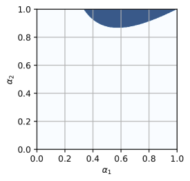
Figure 6. Feasible set for Example 4.11, projected onto $\alpha_{1}\mathchar 44\relax\nolinebreak[3]\alpha_{2}$ for $r=\frac{1}{4}$.

Interestingly, the exact asymptotic is $\Theta((2\sqrt{r(1-r)})^{n}\cdot n^{-3/2})$ (Appendix B), so the best possible geometric bound is $O((2\sqrt{r(1-r)})^{n})$ and our method can get arbitrarily close to it. We could find a bound on $\mathbb{E}[X_{2}]$ in the same way as in the previous example, but this would be very tedious to do manually. Our implementation (again using loop unrolling before applying the above reasoning) finds the bounds shown in Section 6.4 (for $r=\frac{1}{4}$).

4.5. Properties

4.5.1. Decidability

Note that for any ${\color[rgb]{0,.5,.5}\mathsf{EGD}}\mathopen{}\left(\mathbf{P}\mathchar 44\relax\nolinebreak[3]{\bm{\alpha}}\right)\mathclose{}$ occurring in the semantics, $\mathbf{P}$ is a rational function in entries of initial blocks and decay rates. In fact, it is linear in the entries of initial blocks. Hence the $\preceq$ constraints reduce to polynomial inequality constraints. Note that if we want to find an upper bound, these constraints will contain unknowns, which we have to solve for. Since the existential first-order theory of the reals is decidable, we can solve these constraints.

Theorem 4.12.

Given a program $P$ and a canonical ${\color[rgb]{0,.5,.5}\mathsf{EGD}}\mathopen{}\left(\mathbf{P}\mathchar 44\relax\nolinebreak[3]{\bm{\alpha}}\right)\mathclose{}$, it is decidable whether there is an EGD ${\color[rgb]{0,.5,.5}\mathsf{EGD}}\mathopen{}\left(\mathbf{Q}\mathchar 44\relax\nolinebreak[3]{\bm{\beta}}\right)\mathclose{}$ such that ${\color[rgb]{0,.5,.5}\mathsf{EGD}}\mathopen{}\left(\mathbf{P}\mathchar 44\relax\nolinebreak[3]{\bm{\alpha}}\right)\mathclose{}\mathrel{\llbracket P\rrbracket^{\mathsf{geo}}}{\color[rgb]{0,.5,.5}\mathsf{EGD}}\mathopen{}\left(\mathbf{Q}\mathchar 44\relax\nolinebreak[3]{\bm{\beta}}\right)\mathclose{}$.

This is yet another reason to prefer EGDs over more general classes of distributions: while it may be possible to check $\preceq$ for slightly more complicated classes of distributions with concrete values, solving such a system of $\preceq$-inequalities with unknown values will be much harder. Despite the decidability results, solving our constraints is still not easy because the existential theory of the reals is NP-hard and algorithms only work for small instances in practice.

One might hope that the constraints arising from the geometric bound semantics have nice properties. For example, one might expect the solution set $(\mathbf{Q}\mathchar 44\relax\nolinebreak[3]{\bm{\beta}})$ to be convex and ${\bm{\beta}}$ to be right-closed, i.e. that for any solution ${\color[rgb]{0,.5,.5}\mathsf{EGD}}\mathopen{}\left(\mathbf{Q}\mathchar 44\relax\nolinebreak[3]{\bm{\beta}}\right)\mathclose{}$ and any ${\bm{\gamma}}\geq{\bm{\beta}}$, there is a solution ${\color[rgb]{0,.5,.5}\mathsf{EGD}}\mathopen{}\left(\mathbf{Q}^{\prime}\mathchar 44\relax\nolinebreak[3]{\bm{\gamma}}\right)\mathclose{}$, because this weakens the bound. However, we found simple counterexamples to both properties (see Example B.2). We address the problem of practical constraint solving in Section 5.1.

4.5.2. Soundness

We prove that the geometric bound semantics is correct with respect to the standard semantics.

Theorem 4.13 (Soundness).

Let ${\color[rgb]{0,.5,.5}\mathsf{EGD}}\mathopen{}\left(\mathbf{P}\mathchar 44\relax\nolinebreak[3]{\bm{\alpha}}\right)\mathclose{}$ be canonical. The rules for the EGD event semantics (Fig. 4) agree with the standard event semantics: $\left.{\color[rgb]{0,.5,.5}\mathsf{EGD}}\mathopen{}\left(\mathbf{P}\mathchar 44\relax\nolinebreak[3]{\bm{\alpha}}\right)\mathclose{}\right|_{E}^{\mathsf{geo}}={\color[rgb]{0,.5,.5}\mathsf{EGD}}\mathopen{}\left(\mathbf{P}\mathchar 44\relax\nolinebreak[3]{\bm{\alpha}}\right)\mathclose{}|_{E}$. The rules for the EGD statement semantics $\mathrel{\llbracket-\rrbracket^{\mathsf{geo}}}$ (Fig. 5) are sound: if ${\color[rgb]{0,.5,.5}\mathsf{EGD}}\mathopen{}\left(\mathbf{P}\mathchar 44\relax\nolinebreak[3]{\bm{\alpha}}\right)\mathclose{}\mathrel{\llbracket P\rrbracket^{\mathsf{geo}}}{\color[rgb]{0,.5,.5}\mathsf{EGD}}\mathopen{}\left(\mathbf{Q}\mathchar 44\relax\nolinebreak[3]{\bm{\beta}}\right)\mathclose{}$ then $\llbracket P\rrbracket({\color[rgb]{0,.5,.5}\mathsf{EGD}}\mathopen{}\left(\mathbf{P}\mathchar 44\relax\nolinebreak[3]{\bm{\alpha}}\right)\mathclose{})\preceq{\color[rgb]{0,.5,.5}\mathsf{EGD}}\mathopen{}\left(\mathbf{Q}\mathchar 44\relax\nolinebreak[3]{\bm{\beta}}\right)\mathclose{}$ and ${\color[rgb]{0,.5,.5}\mathsf{EGD}}\mathopen{}\left(\mathbf{Q}\mathchar 44\relax\nolinebreak[3]{\bm{\beta}}\right)\mathclose{}$ is canonical. Furthermore, if $\mu={\color[rgb]{0,.5,.5}\mathsf{EGD}}\mathopen{}\left(\mathbf{P}\mathchar 44\relax\nolinebreak[3]{\bm{\alpha}}\right)\mathclose{}$ is a finite subprobability distribution (in particular, ${\bm{\alpha}}=\mathbf{0}_{n}$), then we can bound the normalized distribution:

$$\frac{\llbracket P\rrbracket_{\mathsf{lo}}(\mu)|_{\mathbb{N}^{n}}}{{\color[rgb]{0,.5,.5}\mathsf{EGD}}\mathopen{}\left(\mathbf{Q}\mathchar 44\relax\nolinebreak[3]{\bm{\beta}}\right)\mathclose{}(\mathbb{N}^{n})}\preceq\operatorname{normalize}(\llbracket P\rrbracket_{\lightning}(\mu))\preceq\frac{{\color[rgb]{0,.5,.5}\mathsf{EGD}}\mathopen{}\left(\mathbf{Q}\mathchar 44\relax\nolinebreak[3]{\bm{\beta}}\right)\mathclose{}}{1-\mu(\mathbb{N}^{n})+\llbracket P\rrbracket_{\mathsf{lo}}(\mu)(\mathbb{N}^{n})}$$

4.5.3. Loop-free fragment

It is instructive to look at when $\mathrel{\llbracket-\rrbracket^{\mathsf{geo}}}$ is precise, i.e. when the right-hand side of the relation is unique and equals the $\llbracket-\rrbracket$ semantics. It turns out that this is the case for programs without loops, which is easy to see from the soundness proof.

Theorem 4.14 (Precision for loop-free fragment).

Let $P$ be a loop-free program. Assume that the strict $\mathsf{Join}^{*}$ relation is used in the $\mathrel{\llbracket-\rrbracket^{\mathsf{geo}}}$ semantics of ${\color[rgb]{.5,0,.5}\mathsf{if}}\,{-}\,\allowbreak\{-\}\,\allowbreak{\color[rgb]{.5,0,.5}\mathsf{else}}\,\{-\}$. Then for all canonical ${\color[rgb]{0,.5,.5}\mathsf{EGD}}\mathopen{}\left(\mathbf{P}\mathchar 44\relax\nolinebreak[3]{\bm{\alpha}}\right)\mathclose{}$, there is a unique (also canonical) ${\color[rgb]{0,.5,.5}\mathsf{EGD}}\mathopen{}\left(\mathbf{Q}\mathchar 44\relax\nolinebreak[3]{\bm{\beta}}\right)\mathclose{}$ such that ${\color[rgb]{0,.5,.5}\mathsf{EGD}}\mathopen{}\left(\mathbf{P}\mathchar 44\relax\nolinebreak[3]{\bm{\alpha}}\right)\mathclose{}\mathrel{\llbracket P\rrbracket^{\mathsf{geo}}}{\color[rgb]{0,.5,.5}\mathsf{EGD}}\mathopen{}\left(\mathbf{Q}\mathchar 44\relax\nolinebreak[3]{\bm{\beta}}\right)\mathclose{}$ and $\llbracket P\rrbracket({\color[rgb]{0,.5,.5}\mathsf{EGD}}\mathopen{}\left(\mathbf{P}\mathchar 44\relax\nolinebreak[3]{\bm{\alpha}}\right)\mathclose{})={\color[rgb]{0,.5,.5}\mathsf{EGD}}\mathopen{}\left(\mathbf{Q}\mathchar 44\relax\nolinebreak[3]{\bm{\beta}}\right)\mathclose{}$. Furthermore, each $\beta_{i}\in\{0\mathchar 44\relax\nolinebreak[3]\alpha_{i}\}$.

4.5.4. Sufficient conditions for the existence of bounds

When does the constraint problem arising from our semantics actually have a solution? This is hard to characterize in general because the feasible region can be complex, as discussed above. Furthermore, a useful purely syntactic criterion is unlikely to exist because even for the simple asymmetric random walk ${\color[rgb]{.5,0,.5}\mathsf{while}}\,{X_{1}>0}\,\allowbreak\{{\color[rgb]{.5,0,.5}\mathsf{if}}\,{{\color[rgb]{.5,0,.5}\mathsf{flip}}(\rho)}\,\allowbreak\{X_{1}\mathbin{{+}{=}}1\}\,\allowbreak{\color[rgb]{.5,0,.5}\mathsf{else}}\,\{X_{1}\mathbin{{\dot{-}}{=}}1\}\}$, a bound can be found if and only if $\rho<\frac{1}{2}$.

Nevertheless, we have succeeded in identifying a sufficient criterion for the existence of an EGD loop bound: roughly speaking, if the difference between new and old values of the variables is the same in each loop iteration, and if there is a linear ranking supermartingale (Chatterjee et al., 2016), then an EGD bound exists. The precise conditions are stated in the following theorem.

Theorem 4.15.

Suppose $L={\color[rgb]{.5,0,.5}\mathsf{while}}\,{E}\,\allowbreak\{B\}$ satisfies the following properties:

1. $B$ only contains increment and decrement statements ($X_{k}\mathbin{{+}{=}}1$, $X_{k}\mathbin{{\dot{-}}{=}}1$), probabilistic branching (${\color[rgb]{.5,0,.5}\mathsf{if}}\,{{\color[rgb]{.5,0,.5}\mathsf{flip}}(\dots)}\,\allowbreak\{\dots\}\,\allowbreak{\color[rgb]{.5,0,.5}\mathsf{else}}\,\{\dots\}$), and ${\color[rgb]{.5,0,.5}\mathsf{fail}}$,

2. $E$ occurring guarantees that $X_{1}\geq a_{1}\land\dots\land X_{n}\geq a_{n}$ where $a_{i}\in\mathbb{N}$ is the maximum number of decrements of $X_{i}$ in any program path through $B$, and

3. there is a conical (linear with nonnegative coefficients) combination $\sum_{i=1}^{n}\lambda_{i}X_{i}$ whose expected value decreases after every loop iteration for any initial assignment ${\bm{x}}$ that can enter the loop: $\mathbb{E}_{{\bm{X}}\sim\llbracket B\rrbracket({\color[rgb]{0,.5,.5}\mathsf{Dirac}}({\bm{x}})|_{E})}\left[\sum_{i=1}^{n}\lambda_{i}X_{i}\right]<\sum_{i=1}^{n}\lambda_{i}x_{i}\quad\text{for all }{\bm{x}}\in\mathbb{N}^{n}\text{ with }x_{i}\geq a_{i}$

Then, for any initial canonical ${\color[rgb]{0,.5,.5}\mathsf{EGD}}\mathopen{}\left(\mathbf{P}\mathchar 44\relax\nolinebreak[3]{\bm{\alpha}}\right)\mathclose{}$, there is a solution $(\mathbf{Q}\mathchar 44\relax\nolinebreak[3]{\bm{\beta}})$ to ${\color[rgb]{0,.5,.5}\mathsf{EGD}}\mathopen{}\left(\mathbf{P}\mathchar 44\relax\nolinebreak[3]{\bm{\alpha}}\right)\mathclose{}\mathrel{\llbracket L\rrbracket^{\mathsf{geo}}}{\color[rgb]{0,.5,.5}\mathsf{EGD}}\mathopen{}\left(\mathbf{Q}\mathchar 44\relax\nolinebreak[3]{\bm{\beta}}\right)\mathclose{}$.

Although the assumptions of this theorem may seem restrictive, they are sufficient to prove the existence of bounds for the random walk (Example 4.11), which is nontrivial to analyze. In that case, $a_{1}=1\mathchar 44\relax\nolinebreak[3]a_{2}=0$ and the expected value of $X_{1}$ decreases by $1-2r>0$ in each loop iteration.

4.5.5. Necessary conditions for the existence of bounds

We already mentioned that the existence of bounds is not guaranteed in general. An obvious necessary condition is that the true program distribution actually has tails that decay exponentially fast, i.e. can be bounded by an EGD. It turns out that the same must hold for the running time of the program as well.

Theorem 4.16 (Necessary conditions on the running time).

If ${\color[rgb]{0,.5,.5}\mathsf{EGD}}\mathopen{}\left(\mathbf{P}\mathchar 44\relax\nolinebreak[3]{\bm{\alpha}}\right)\mathclose{}\mathrel{\llbracket P\rrbracket^{\mathsf{geo}}}{\color[rgb]{0,.5,.5}\mathsf{EGD}}\mathopen{}\left(\mathbf{Q}\mathchar 44\relax\nolinebreak[3]{\bm{\beta}}\right)\mathclose{}$ for a canonical ${\color[rgb]{0,.5,.5}\mathsf{EGD}}\mathopen{}\left(\mathbf{P}\mathchar 44\relax\nolinebreak[3]{\bm{\alpha}}\right)\mathclose{}$ then the running time $T$ of $P$ on ${\color[rgb]{0,.5,.5}\mathsf{EGD}}\mathopen{}\left(\mathbf{P}\mathchar 44\relax\nolinebreak[3]{\bm{\alpha}}\right)\mathclose{}$ can be bounded by an EGD as well. In particular, all its moments $\mathbb{E}[T^{k}]$ must be finite.

4.5.6. Loop unrolling and convergence

Just like for the residual mass semantics, we would expect the geometric bound semantics to yield tighter and tighter bounds as we unroll loops further and further. It turns out that for the $u$-fold unrolling $P^{(u)}$ of a program $P$, we can find upper bounds whose distance from the true distribution decreases exponentially in $u$.

Theorem 4.17 (Convergence).

Let $P$ be a program containing potentially nested loops and $P^{(u)}$ its $u$-fold unrolling. Suppose ${\color[rgb]{0,.5,.5}\mathsf{EGD}}\mathopen{}\left(\mathbf{P}\mathchar 44\relax\nolinebreak[3]{\bm{\alpha}}\right)\mathclose{}\mathrel{\llbracket P\rrbracket^{\mathsf{geo}}}{\color[rgb]{0,.5,.5}\mathsf{EGD}}\mathopen{}\left(\mathbf{Q}\mathchar 44\relax\nolinebreak[3]{\bm{\beta}}\right)\mathclose{}$ for a canonical ${\color[rgb]{0,.5,.5}\mathsf{EGD}}\mathopen{}\left(\mathbf{P}\mathchar 44\relax\nolinebreak[3]{\bm{\alpha}}\right)\mathclose{}$. Then there exist $A\in\mathbb{\mathbb{R}}_{\geq 0}\mathchar 44\relax\nolinebreak[3]C\in[0\mathchar 44\relax\nolinebreak[3]1)$ and $\mathbf{Q}^{(u)}$ such that ${\color[rgb]{0,.5,.5}\mathsf{EGD}}\mathopen{}\left(\mathbf{P}\mathchar 44\relax\nolinebreak[3]{\bm{\alpha}}\right)\mathclose{}\mathrel{\llbracket P^{(u)}\rrbracket^{\mathsf{geo}}}{\color[rgb]{0,.5,.5}\mathsf{EGD}}\mathopen{}\left(\mathbf{Q}^{(u)}\mathchar 44\relax\nolinebreak[3]{\bm{\beta}}\right)\mathclose{}\preceq{\color[rgb]{0,.5,.5}\mathsf{EGD}}\mathopen{}\left(\mathbf{Q}\mathchar 44\relax\nolinebreak[3]{\bm{\beta}}\right)\mathclose{}$ and

$${\color[rgb]{0,.5,.5}\mathsf{EGD}}\mathopen{}\left(\mathbf{Q}^{(u)}\mathchar 44\relax\nolinebreak[3]{\bm{\beta}}\right)\mathclose{}-\llbracket P\rrbracket({\color[rgb]{0,.5,.5}\mathsf{EGD}}\mathopen{}\left(\mathbf{P}\mathchar 44\relax\nolinebreak[3]{\bm{\alpha}}\right)\mathclose{})\preceq A\cdot C^{u}\cdot{\color[rgb]{0,.5,.5}\mathsf{EGD}}\mathopen{}\left(\mathbf{Q}\mathchar 44\relax\nolinebreak[3]{\bm{\beta}}\right)\mathclose{}$$

In particular, the distribution bound ${\color[rgb]{0,.5,.5}\mathsf{EGD}}\mathopen{}\left(\mathbf{Q}^{(u)}\mathchar 44\relax\nolinebreak[3]{\bm{\beta}}\right)\mathclose{}$ converges in total variation distance to the true distribution $\llbracket P\rrbracket({\color[rgb]{0,.5,.5}\mathsf{EGD}}\mathopen{}\left(\mathbf{P}\mathchar 44\relax\nolinebreak[3]{\bm{\alpha}}\right)\mathclose{})$, as $u\to\infty$. Similarly, for any $k$, the $k$-th moment bound $\mathbb{E}_{{\bm{X}}\sim{\color[rgb]{0,.5,.5}\mathsf{EGD}}\mathopen{}\left(\mathbf{Q}^{(u)}\mathchar 44\relax\nolinebreak[3]{\bm{\beta}}\right)\mathclose{}}[X_{i}^{k}]$ converges to the true moment $\mathbb{E}_{{\bm{X}}\sim\llbracket P\rrbracket({\color[rgb]{0,.5,.5}\mathsf{EGD}}\mathopen{}\left(\mathbf{P}\mathchar 44\relax\nolinebreak[3]{\bm{\alpha}}\right)\mathclose{})}[X_{i}^{k}]$.

Note that this theorem does not prove that the parameters ${\bm{\beta}}$ of the geometric tails converge to the best possible ones. In general, unrolling does not improve the decay rate at all, except for specific cases where the loop is finite and can be fully unrolled. In fact, the derived tail bounds may differ arbitrarily from the true tails, as shown in the next example.

Example 4.18 (Nonoptimal tail bounds).

As an example of nonoptimal tail bounds, consider the following program where $\rho\in(0\mathchar 44\relax\nolinebreak[3]1)$:

$$X_{1}:=0;X_{2}:=0;$$

$${\color[rgb]{.5,0,.5}\mathsf{while}}\,{{\color[rgb]{.5,0,.5}\mathsf{flip}}(\rho)}\,\allowbreak\{X_{1}\mathbin{{+}{=}}1;X_{2}\mathbin{{+}{=}}1\};$$

$${\color[rgb]{.5,0,.5}\mathsf{while}}\,{X_{1}>0\land X_{2}>0}\,\allowbreak\{X_{1}\mathbin{{\dot{-}}{=}}1;X_{2}\mathbin{{\dot{-}}{=}}1\}$$

It is clear that at the end of the program, $X_{1}=0$ and $X_{2}=0$ almost surely. Throughout the program, the same operations are applied to them. However, the geometric bound semantics cannot keep track of this correlation completely because the structure of EGDs can only express correlations in the finite initial block and not in the tails. Hence the best tail bounds we get for $X_{1}$ and $X_{2}$ are of the form $O((\rho+\delta)^{n})$ for any $\delta>0$, whereas the true tails are zero. So the tail bounds can be arbitrarily far from the true tails. Note, however, that the existence of geometric tails is already useful knowledge: it tells us that the distribution is not heavy-tailed and that all moments are finite.

5. Implementation

We implemented both the residual mass semantics and the geometric bound semantics in a tool called Diabolo (“Discrete Distribution Analysis via Bounds, supporting Loops and Observations”). The code is available at github.com/fzaiser/diabolo and on Zenodo (Zaiser, 2024a).

Diabolo takes a probabilistic program as input and outputs bounds on probability masses, moments, and tail asymptotics of the posterior distribution of a specified program variable. The output and computational effort can be controlled with various options. The most important one is the loop unrolling limit $u$, which is common to both semantics. The geometric bound semantics has additional options: the dimension $d$ of the contraction invariants to be synthesized, an optimization objective, as well as the solver and optimizer to be used for the polynomial constraints. The optimization objective is the quantity whose bound should be optimized: the probability mass, the expected value, or the asymptotic decay rates. Depending on which of these is chosen, the best EGD bound can vary significantly (see Section 4.4). Diabolo is implemented in Rust (Matsakis and Klock II, 2014) for performance and uses exact rational number computations instead of floating point to ensure the correctness of the results. We describe a few practical aspects of the implementation below, most of them pertaining to the geometric bound semantics.

Nondeterminism in the semantics

As pointed out in Section 4.3, there are two places in the geometric bound semantics where choices have to be made: branching and loops. To generate the polynomial constraints arising from ${\color[rgb]{.5,0,.5}\mathsf{while}}$ loops, we need to choose the size of the contraction invariants ${\color[rgb]{0,.5,.5}\mathsf{EGD}}\mathopen{}\left(\mathbf{R}\mathchar 44\relax\nolinebreak[3]{\bm{\gamma}}\right)\mathclose{}$. It is usually best to choose the dimensions of $\mathbf{R}$ to be as small as possible (often 1): this reduces both the number of constraints and constraint variables, which facilitates solving. Some programs only have larger contraction invariants, but the dimension rarely needs to be greater than 2. In terms of quality of the bounds, increasing the unrolling limit has a much greater effect (cf. Theorem 4.17). In the semantics of ${\color[rgb]{.5,0,.5}\mathsf{if}}$ statements, the choice is in the size of the expansion of the EGDs in the $\mathsf{Join}$ relation. In Diabolo, we choose the smallest expansion for speed and memory usage reasons. The size of the EGDs depends mostly on the size of the contraction invariant, so an increase there automatically reduces the imprecision in $\mathsf{Join}$.

Approximating the support

In the constraint problem arising from a $c$-contraction invariant ${\color[rgb]{0,.5,.5}\mathsf{EGD}}\mathopen{}\left(\mathbf{R}\mathchar 44\relax\nolinebreak[3]{\bm{\gamma}}\right)\mathclose{}$, the constraint variables corresponding to the entries of $\mathbf{R}$ are “easy” because they only occur linearly, whereas the constraints typically contain higher-degree polynomials in ${\bm{\gamma}}$. For this reason, it is desirable to determine the decay rates ${\bm{\gamma}}$ in advance, if possible. If the program variable $X_{i}$ has finite support $\{a_{i}\mathchar 44\relax\nolinebreak[3]a_{i}+1\mathchar 44\relax\nolinebreak[3]\dots\mathchar 44\relax\nolinebreak[3]b_{i}\}\subset\mathbb{N}$, we can set the decay rate $\gamma_{i}$ to zero (since the tails of $X_{i}$’s distribution are zero). But to be able to represent its distribution with $\gamma_{i}=0$, we have to choose at least $|\mathbf{R}|_{i}=b_{i}+1$. (In this case, the user-provided dimension $d$ for the contraction invariant is overridden.) Furthermore, we can infer from the support that $\mathbf{R}_{i:j}=\mathbf{0}$ for $j<a_{i}$. To reap these benefits, we need to analyze the support of the random variables occurring in the program. This is a standard application of abstract interpretation on the interval domain. Overapproximating the support also has the benefit that we automatically know that probabilities outside of it are zero, which can improve the results of both semantics (see Section C.1).

5.1. Constraint solving

How can we solve the polynomial constraints arising from the geometric bound semantics? As this is a decidable problem known as the existential theory of the reals, we first tried to use SMT solvers, such as Z3 (de Moura and Bjørner, 2008) and CVC5 (Barbosa et al., 2022), and the dedicated tool QEPCAD (Brown, 2003). Out of these, Z3 performed the best, but it was only able to solve the simplest problems and scaled badly.

Numerical solvers

Given that even simple programs lead to dozens and sometimes hundreds of constraints, we resorted to numerical solutions instead. The best solver for our purposes turned out to be IPOPT: a library for large-scale nonlinear optimization (Wächter and Biegler, 2006). One issue with IPOPT are rounding errors, so it sometimes returns solutions that are not exactly feasible. To address this, we tighten the constraints by a small margin before handing them over to IPOPT and check the feasibility of the returned solution with exact rational arithmetic. Another disadvantage of IPOPT is that it cannot prove infeasibility – only exact solvers like Z3 and QEPCAD can do so. However, its impressive scalability makes up for these shortcomings.

We also developed a custom solver that transforms the constraint problem into an unconstrained optimization problem (details in Section C.2) and applies the ADAM optimizer (Kingma and Ba, 2015), a popular gradient descent method. We also explored other off-the-shelf solvers for polynomial constraints: IBEX, a rigorous solver based on interval arithmetic, and constrained optimization methods in scipy, the Python scientific computing library; but neither of them performed well. Diabolo includes the solvers IPOPT (the default), our ADAM-based solver, and Z3.

Nested loops

Nested loops are an interesting special case for numerical solvers. They lead to cyclic $\leq$-constraints on the decay rates, e.g. $\alpha\leq\beta\land\beta\leq\alpha$. Numerical solvers struggle with such indirect equality constraints, so we added a preprocessing step to detect them and replace the equal variables with a single representative.

Reducing the cost of unrolling

Unrolling loops is essential to obtain close bounds on posterior masses and moments (it does not affect tail bounds). On the other hand, unrolling increases the complexity of the constraint problem considerably, both in terms of number of variables and constraints. A key observation from Theorem 4.17 can mitigate this problem: the variables that occur nonlinearly, i.e. decay rates and contraction factors, need not be changed as the unrolling count increases. As a consequence, we first solve the constraint problem without unrolling and need only solve a linear constraint problem for higher unrolling limits. Since linear programming solvers are much faster and more robust than nonlinear solvers, this approach significantly reduces numerical issues and computation time. In fact, without this technique, several benchmarks in Section 6.1 would not be solvable at all.

5.2. Optimization

Since the geometric bound semantics is nondeterministic, there are many EGD bounds for a given program. Which one is the best depends on what quantity we want to optimize. In Diabolo, the user can specify one of the following optimization objectives to minimize: the bound on the total probability mass, on the expected value, or on the tail asymptotics (i.e. decay rate).

IPOPT and the ADAM-based solver can also be used for optimization. Moreover, we apply the linear programming solver CBC by the COIN-OR project to optimize the linear variables (keeping the nonlinear ones fixed), which is very fast. By default, Diabolo runs IPOPT, the ADAM-based optimizer, and the linear solver in this order, each improving the solution of the previous one. The ADAM-based optimizer can be slow for larger programs, in which case the user may decide to skip it. However, it often finds better tail bounds than IPOPT, which is why it is included by default.

6. Empirical Evaluation

In this section, we evaluate our two methods in practice to answer the following four questions:

1. How often is the geometric bound semantics applicable in practice? (Section 6.1)

2. How tight are the bounds in practice? (Section 6.2)

3. How do our methods perform compared to previous work? (Section 6.3)

4. How do our two semantics perform compared to each other? (Section 6.4)

All benchmarks and code to reproduce the results are available (Zaiser, 2024a).

6.1. Applicability of the geometric bound semantics

In this section, we empirically investigate the existence of geometric bounds, i.e. how often the constraints arising from the geometric bound semantics can be solved. If some bound can be found at all, Theorem 4.17 ensures that it can be made arbitrarily tight by increasing the unrolling limit. (This aspect of the quality of bounds is studied in Sections 6.2 and 6.4.) While Theorem 4.15 provides sufficient conditions for existence, we want to test the applicability of the geometric bound semantics in practice in a systematic way.

Benchmark selection

For this purpose, we collected benchmarks from the Github repositories of several probabilistic programming languages: Polar (Moosbrugger et al., 2022), Prodigy (Klinkenberg et al., 2024), and PSI (Gehr et al., 2016). Note that a benchmark being available in a tool’s repository does not mean that the tool can solve it. We searched all benchmarks from these repositories for the keyword while, in order to find benchmarks with loops. We manually filtered out benchmarks whose loops are actually bounded or that make essential use of continuous distributions (15), negative integers (4), comparisons of two variables (7), or multiplication (1), because our language cannot express these. Some benchmarks using these features could still be translated in other ways to an equivalent program in our language.

We ended up with 43 benchmarks: 9 from Polar, 11 from Prodigy, 9 from PSI, and we added 14 of our own. They include standard probabilistic loop examples (in particular, all examples from this paper, and variations thereof), nested loops, and real-world algorithms, such as probabilistic self-stabilization protocols (Herman, 1990; Israeli and Jalfon, 1990; Beauquier et al., 1999).

Symbolic inputs

Polar and Prodigy can handle symbolic inputs and symbolic parameters to some extent, which our techniques cannot. One benchmark (polar/fair_biased_coin) used symbolic parameters, which we replaced with concrete values. Several benchmarks from Polar and Prodigy have symbolic inputs, i.e. they are parametric in the initial values in $\mathbb{N}$ of the variables. Since our method cannot reason parametrically about the input, we instead put a ${\color[rgb]{0,.5,.5}\mathsf{Geometric}}(1/2)$ distribution on such inputs, to cover all possible values. Of course, this yields less information than a method computing a symbolic result that is valid for all input values. But if an EGD bound can be found for this input distribution, then an EGD bound can be found for each possible input value because any Dirac distribution on the input can be bounded by a scaled version of the geometric distribution: ${\color[rgb]{0,.5,.5}\mathsf{Dirac}}(m)\preceq 2^{m}\cdot{\color[rgb]{0,.5,.5}\mathsf{Geometric}}(1/2)$. Thus, for the question of the existence of bounds, we consider this a valid approach. Note that reasoning about such a geometric distribution on the input is nontrivial (and much harder than reasoning about fixed input values). For instance, Polar cannot always handle it even for benchmarks where it supports the version with symbolic input values.

Methodology

We ran our tool Diabolo for the geometric bound semantics on all benchmarks with a timeout of 5 minutes. The configuration options were mostly left at the defaults for most benchmarks (invariant size: 1, solver: IPOPT). However, we disabled unrolling for all benchmarks since it only affects the quality of bounds, not their existence. For 4 benchmarks, the invariant size had to be increased to 2 or 3 to find bounds. For each benchmark, we recorded the time it took to compute the bounds, or any errors.

Results

Diabolo was able to solve 37 out of the 43 benchmarks (86%); 5 failed because no EGD bound exists (at least 3 of them have infinite expected running time); and 1 timed out due to the complexity of the constraint problem. Among the solved benchmarks, the solution time was at most 3 seconds and typically much less. This demonstrates that our geometric bound semantics is also of practical relevance, in addition to its nice theoretical properties. Detailed results are available in Table 6 (Appendix D), along with statistics about the input program and the constraint problem arising from the geometric bound semantics.

6.2. Quality of the geometric bounds

Table 2. Diabolo’s bounds on the expected value and the tail asymptotics for the benchmarks from Section 6.1 where bounds exist. Results are rounded to 4 significant digits. (#U: unrolling limit; EV: expected value; “?”: ground truth could not be determined; “†”: could not be solved by an automatic tool before, in the sense of bounding the distribution’s moments and tails without user intervention; timeout: 5 minutes exceeded.)

Benchmark	#U	True EV	EV bound	Time	True tail	Tail bound	Time
polar/c4B_t303 †	30	0.1787…	[0.1787, 0.1788]	0.24 s	?	$O(0.5001^{n})$	0.12 s
polar/coupon_collector2	30	2	[1.999, 2.001]	0.16 s	$\Theta(0.5^{n})$	$O(0.5071^{n})$	0.11 s
polar/fair_biased_coin	30	0.5	[0.4999, 0.5001]	0.03 s	$0$	$0$	0.02 s
polar/las_vegas_search	200	20	[19.98, 26.79]	2.29 s	$\Theta(0.9523...^{n})$	$O(0.9524^{n})$	0.72 s
polar/linear01 †	30	0.375	[0.3749, 0.3751]	0.03 s	$0$	$0$	0.03 s
polar/simple_loop	30	1.3	[1.299, 1.301]	0.02 s	$0$	$0$	0.02 s
prodigy/bit_flip_conditioning	30	1.254…	[1.254, 1.255]	0.28 s	?	$O(0.6254^{n})$	0.19 s
prodigy/brp_obs †	30	4.989…e-10	[4.989e-10, 1.489e-09]	0.61 s	$0$	$0$	3.83 s
prodigy/condand †	30	0.75	[0.7499, 0.7501]	0.15 s	?	$O(0.5001^{n})$	0.07 s
prodigy/dep_bern †	30	0.5	[0.4999, 0.5124]	1.00 s	$\Theta(0.3333...^{n})$	$O(0.34^{n})$	0.17 s
prodigy/endless_conditioning	30	undef	undef	0.15 s	$0$	$0$	0.13 s
prodigy/geometric	30	2	[1.999, 2.007]	1.09 s	$\Theta(0.5^{n})$	$O(0.5066^{n})$	0.60 s
prodigy/ky_die	30	3.5	[3.499, 3.501]	0.18 s	$0$	$0$	0.08 s
prodigy/n_geometric †	30	1	[0.998, 1.068]	0.08 s	$\Theta(0.6666...^{n})$	$O(0.673^{n})$	0.07 s
prodigy/trivial_iid †	30	3.5	[3.499, 3.503]	2.60 s	$\Theta(0.8318...^{n})$	$O(0.836^{n})$	0.16 s
psi/beauquier-etal3	30	?	✗ (timeout)	t/o	?	$O(0.7952^{n})$	17.64 s
psi/cav-example7	80	10.41…	[10.41, 10.51]	1.71 s	?	$O(0.8927^{n})$	0.12 s
psi/dieCond (Ex. 1.1) †	40	1.5	[1.499, 1.501]	0.15 s	$\Theta(0.3333...^{n})$	$O(0.3395^{n})$	0.13 s
psi/ex3	30	0.6666…	[0.6666, 0.6667]	0.04 s	$0$	$0$	0.06 s
psi/ex4	30	0.6666…	[0.6666, 0.6667]	0.23 s	$0$	$0$	0.27 s
psi/fourcards	30	0.2642…	[0.264, 0.2648]	0.46 s	$0$	$0$	0.34 s
psi/herman3	30	1.333…	[1.333, 1.334]	62.08 s	?	$O(0.5002^{n})$	0.48 s
psi/israeli-jalfon3	30	0.6666…	[0.6666, 0.6668]	1.71 s	?	$O(0.2501^{n})$	0.15 s
psi/israeli-jalfon5	30	?	✗ (timeout)	t/o	?	$O(0.6583^{n})$	7.13 s
ours/1d-asym-rw (Ex. 4.11) †	70	2	[1.999, 2.542]	1.47 s	$\Theta(\frac{0.8660...^{n}}{n^{1.5}})$	$O(0.8682^{n})$	0.12 s
ours/2d-asym-rw †	70	?	[7.394, 100.4]	79.60 s	?	$O(0.9385^{n})$	4.88 s
ours/3d-asym-rw †	30	?	[9.443, 6.85e+05]	289.94 s	?	$O(0.9812^{n})$	6.35 s
ours/asym-rw-conditioning †	70	2.444…	[2.316, 2.588]	4.85 s	$0$	$0$	0.05 s
ours/coupon-collector5	80	11.41…	[11.41, 11.56]	47.93 s	$\Theta(0.8^{n})$	$O(0.8002^{n})$	15.56 s
ours/double-geo (Ex. B.2) †	30	2	[1.999, 2.01]	0.32 s	$\Theta(0.7071...^{n})$	$O(0.711^{n})$	0.12 s
ours/geometric (Ex. 4.10) †	30	1	[0.9999, 1.006]	0.12 s	$\Theta(0.5^{n})$	$O(0.5037^{n})$	0.10 s
ours/grid †	30	2.75	[2.749, 2.766]	2.39 s	?	$O(0.5285^{n})$	0.30 s
ours/imprecise_tails (Ex. 4.18) †	30	0	[0, 0.007054]	2.36 s	$0$	$O(0.5001^{n})$	0.18 s
ours/israeli-jalfon4	30	?	[1.457, 1.458]	121.04 s	?	$O(0.5011^{n})$	0.44 s
ours/nested †	5	?	[0.9152, 10.57]	12.59 s	?	$O(0.4998^{n})$	0.40 s
ours/sub-geom †	30	0.6666…	[0.6666, 0.6667]	0.06 s	?	$O(0.5001^{n})$	0.10 s
ours/sum-geos	80	8	[7.998, 8.001]	2.91 s	$\Theta(0.875^{n})$	$O(0.8751^{n})$	0.30 s

Methodology

Beyond the mere existence, we are also interested in the quality of the bounds. To this end, we ran Diabolo again on each benchmark where a bound could be found, once optimizing the bound on the expected value, once optimizing the tail bound. The configuration options were left at the default settings for most benchmarks and with an unrolling limit of 30. For expectation bounds, we modified the settings for 23 benchmarks, to adjust the unrolling limit (reported in Table 2), invariant size to 2, 3, or 4 (if smaller values failed or yielded bad bounds), and to skip the ADAM-based optimizer (due to it being slow for some benchmarks). For tail bounds, we set the unrolling limit to 1 and modified the default settings for 15 benchmarks to adjust the invariant size to 2, 3, or 4 and to skip the ADAM-based optimizer (due to it being slow for some benchmarks).

Results

The results are shown in Table 2. We mark with “†” all examples that, to our knowledge, could not be solved automatically before, in the sense of bounding the distribution’s moments and tails without user intervention. Note that no other existing tool is able to obtain exponential tail bounds like ours on any benchmark (unless the tails are zero). One can see that all bounds are nontrivial and the upper and lower bounds on the expected value are usually close together. However, it seems to be harder to find good bounds for benchmarks where the tails of the distribution decay slowly, such as the asymmetric random walks (ours/*-asym-rw). Most of the tail bounds are also very close to the theoretical optimum where the exact tail bound could be manually determined. This demonstrates that our geometric bound semantics generally yields useful bounds.

6.3. Comparison with previous work

Comparison with GuBPI (Beutner et al., 2022)

Our residual mass semantics shares many characteristics with GuBPI (see Table 1). However, GuBPI is designed for a more general setting with continuous sampling and soft conditioning. As a consequence, when applied to discrete probabilistic programs with only hard conditioning, there is a lot of overhead. To demonstrate this, we ran both tools on Examples 4.10, 4.11 and 1.1, configured to produce the same bounds. The results (Table 3) show that Diabolo’s residual mass semantics is several orders of magnitude faster than GuBPI.

Wang et al. (2024) subsequently improved on GuBPI’s results, but we were unable to compare with their system because they use proprietary software. However, they report performance improvements of at most a factor of 15 over GuBPI, which is insufficient to bridge the factor of over 100 for Example 4.10 between GuBPI and our residual mass semantics, let alone the factor of over $10^{5}$ for Example 1.1. This demonstrates that the residual mass semantics is more effective than existing tools for discrete probabilistic programs.

Table 3. Comparison of the running time of GuBPI (Beutner et al., 2022) and our residual mass semantics (as implemented in Diabolo) to produce the same bounds.

Benchmark	GuBPI	Residual mass semantics	Speedup factor
Simple counter (Example 4.10)	0.7 s	0.006 s	$1.2\cdot 10^{2}$
Asymmetric random walk (Example 4.11)	90 s	0.002 s	$4.5\cdot 10^{4}$
Mossel’s die paradox (Example 1.1)	156 s	0.0008 s	$2\cdot 10^{5}$

Table 4. Comparison of Diabolo with Polar (Moosbrugger et al., 2022) on the benchmarks from Table 2 where Polar can compute the expected value (EV). Diabolo’s results are the same as in Table 2, but listed again for an easier comparison. (t/o: timeout of 5 minutes exceeded.)

Benchmark	Polar		Diabolo (ours)
	Exact EV	Time	EV bound	Time
polar/coupon_collector2	2	0.26 s	[1.999, 2.001]	0.16 s
polar/fair_biased_coin	1/2	0.41 s	[0.4999, 0.5001]	0.03 s
polar/las_vegas_search	✗	t/o	[19.98, 26.79]	2.29 s
polar/simple_loop	13/10	0.20 s	[1.299, 1.301]	0.02 s
prodigy/geometric	2	0.46 s	[1.999, 2.007]	1.09 s
prodigy/ky_die	✗	t/o	[3.499, 3.501]	0.18 s
psi/beauquier-etal3	✗	t/o	✗	t/o
psi/cav-example7	✗	t/o	[10.41, 10.51]	1.71 s
psi/ex3	2/3	0.58 s	[0.6666, 0.6667]	0.04 s
psi/ex4	2/3	0.21 s	[0.6666, 0.6667]	0.23 s
psi/fourcards	✗	t/o	[0.264, 0.2648]	0.46 s
psi/herman3	4/3	19.53 s	[1.333, 1.334]	62.08 s
psi/israeli-jalfon3	2/3	19.40 s	[0.6666, 0.6668]	1.71 s
psi/israeli-jalfon5	✗	t/o	✗	t/o
ours/coupon-collector5	137/12	74.86 s	[11.41, 11.56]	47.93 s
ours/geometric	1	0.59 s	[0.9999, 1.006]	0.12 s
ours/israeli-jalfon4	✗	t/o	[1.457, 1.458]	121.04 s
ours/sum-geos	8	0.19 s	[7.998, 8.001]	2.91 s

Comparison with Polar

We compare the geometric bound semantics (as implemented in Diabolo) with Polar (Moosbrugger et al., 2022), the only other tool that can be used to bound moments. In fact, Polar can compute moments exactly, but does not bound the tail asymptotics. We only included benchmarks from Table 2 where Polar can compute the expected value (EV), at least in theory. (We had to extend Polar slightly to support a geometric distribution as the initial distribution.) Polar was run with a timeout of 5 minutes, like Diabolo. The results (Table 4) demonstrate that Diabolo is often faster, and sometimes much faster, than Polar and applicable to more benchmarks.

Comparison of tail bounds

There are several existing program analyses that can bound the tail distribution of the running time of a probabilistic program (see Section 7), but only one (Chatterjee et al., 2016) achieves exponential bounds $O(c^{n})$ for $c<1$ like our bounds. This is particularly interesting as their assumptions (bounded differences and the existence of a linear ranking supermartingale) are remarkably similar to the conditions of our Theorem 4.15. Since the code for the experiments by Chatterjee et al. (2016) is not available, we do a manual comparison on Examples 4.10 and 4.11. Our geometric bound semantics yields the bounds $O((\frac{1}{2}+\varepsilon)^{n})$ and $O((2\sqrt{r(1-r)}+\varepsilon)^{n})$, respectively, whereas their method yields $O((\exp(-1/2))^{n})$ and $O((\sqrt{\exp(-(1-2r)^{2})})^{n})$, where $r$ is the bias of the random walk. It is not hard to see that our bounds are tighter (details in Appendix D).

6.4. Comparison between our two semantics

Table 5. Quality of various bounds in terms of moments and tail bounds for Examples 4.10 and 4.11 using the residual mass and geometric bound semantics.

Example	Method	Expected value	2nd moment	Tail	Time
Simple counter (Example 4.10)	exact	1	3	$\Theta(0.5^{n})$
	res. mass sem.	$\geq 1-5\cdot 10^{-14}$	$\geq 3-3\cdot 10^{-12}$	n/a	0.003 s
	geom. bound sem.	$\leq 1.000037$	$\leq 3.00017$	$O(0.5037^{n})$	0.092 s
Random walk (Example 4.11)	exact	2	10	$\Theta(n^{-3/2}0.8660...^{n})$
	res. mass sem.	$\geq 1.99997$	$\geq 9.998$	n/a	0.067 s
	geom. bound sem.	$\leq 2.55$	$\leq 21.8$	$O(0.8682^{n})$	1.47 s
Introductory “Die paradox” (Example 1.1)	exact	1.5	3	$\Theta(0.3333...^{n})$
	res. mass sem.	$\geq 1.5-2\cdot 10^{-16}$	$\geq 3-4\cdot 10^{-16}$	n/a	0.005 s
	geom. bound sem.	$\leq 1.5+8\cdot 10^{-7}$	$\leq 3+3\cdot 10^{-6}$	$O(0.3395^{n})$	0.097 s
Coupon collector (5 coupons)	exact	11.41666…	155.513888…	$\Theta(0.8^{n})$
	res. mass sem.	$\geq 11.41665$	$\geq 155.5131$	n/a	0.88 s
	geom. bound sem.	$\leq 11.56$	$\leq 158.5$	$O(0.8002^{n})$	22.6 s
Herman’s self-stabilization (3 processes)	exact	1.333…	4.222…	?
	res. mass sem.	$\geq 1.3333332$	$\geq 4.222220$	n/a	0.509 s
	geom. bound sem.	$\leq 1.3339$	$\leq 4.226$	$O(0.5002^{n})$	34.8 s

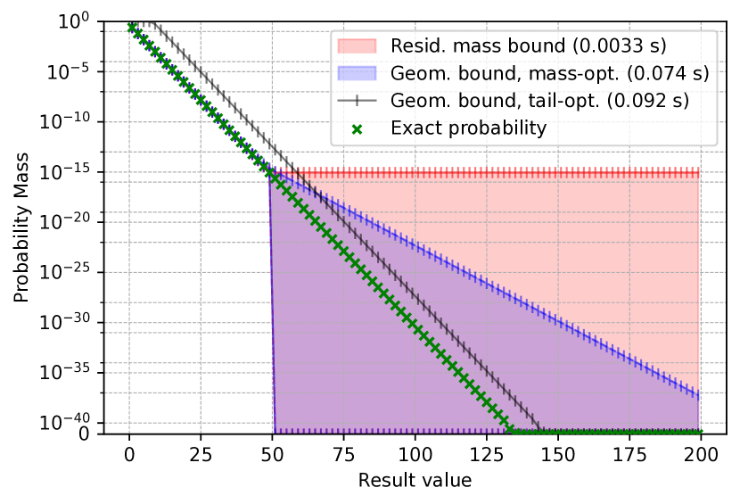
(a) Geom. counter (Example 4.10)

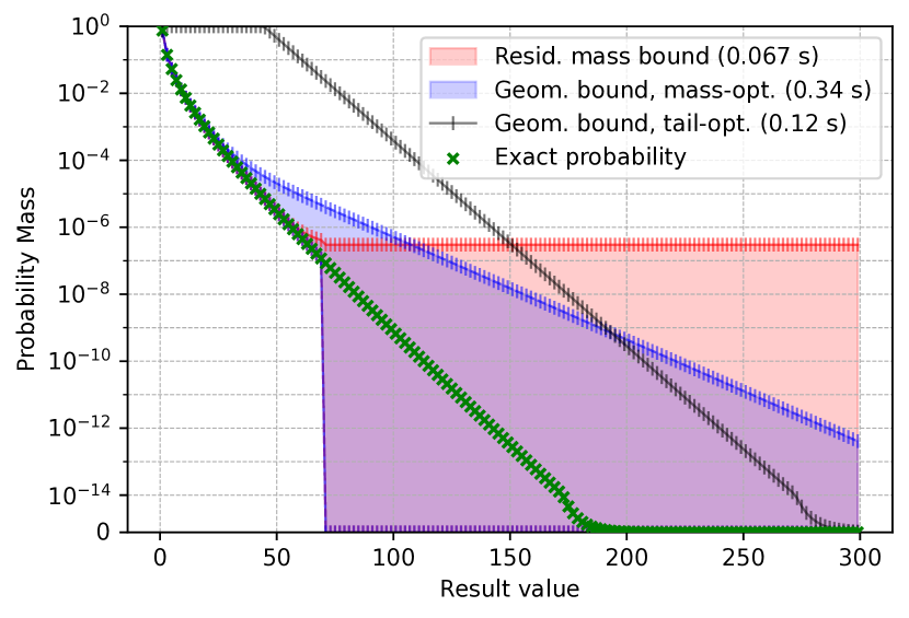
(b) Asym. rand. walk (Example 4.11)

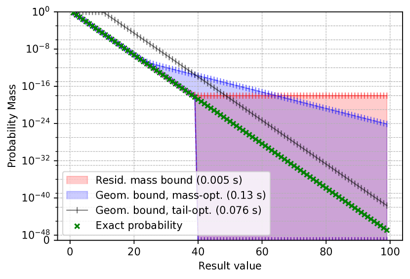
(c) Die paradox (Example 1.1)

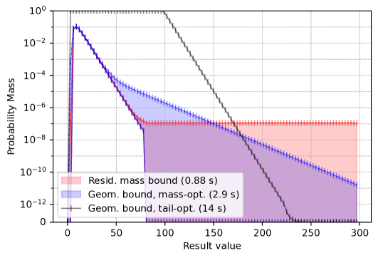
(d) Coupon collector problem with 5 coupons.

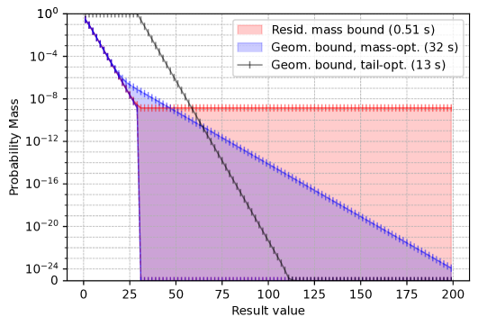
(e) Herman’s self-stabilization with 3 processes.

Figure 7. Comparison of the residual mass and geometric bound semantics. Note that the probability masses (y-axis) are on a logarithmic scale, except for the lowest part, which is linear so as to include 0.

We compare the quality of the bounds from the two semantics on 5 examples: the simple counter (Example 4.10), the asymmetric random walk (Example 4.11), the introductory example (Example 1.1), the coupon collector problem with 5 coupons (ours/coupon-collector5), and Herman’s self-stabilization protocol with 3 processes (adapted from psi/herman3). They were run with a loop unrolling limit of 50, 70, 40, 80, and 30 respectively, except for the geometric tail bounds where the limit was set to 1. We report bounds on the first two (raw) moments and the tails (Section 6.4). Note that the residual mass semantics (not just the lower bound semantics) is needed for lower bounds on moments because they require upper bounds on the normalizing constant. The optimization objective for the EGD bounds was the expected value for the moment bounds and the decay rate for the tail bound. The residual mass semantics is faster and finds good lower bounds on the moments, but cannot find upper bounds or tail bounds. The geometric bound semantics can find upper bounds on both, but takes much more time than the residual mass semantics.

The bounds on the probability masses can be found in Fig. 7. We report EGD bounds for two optimization objectives: the total probability mass (“mass-optimized”) and the decay rate (“tail-optimized”). The residual mass semantics is faster and yields tighter bounds for the probability masses on small values, but the bound is flat, i.e. the difference between upper and lower bounds on probability masses is constant. In contrast, the geometric bound semantics finds upper bounds that keep decreasing like a geometric distribution even for large numbers beyond the unrolling limit. On the other hand, its upper bound is somewhat worse for small values than the residual mass semantics. This is because the geometric bounds arise from the contraction invariant, which requires a uniform decrease of the distribution. So the geometric bounds need to lose precision either for large values (when minimizing the total mass bound), or small values (when minimizing the tail bounds). In fact, the tail-optimized bound is much worse for small values, but eventually becomes almost parallel to the exact solution, since their asymptotics are almost equal up to a constant factor.

7. Related work

A summary of the most relevant work is given in Table 1: guaranteed bounds (Beutner et al., 2022; Wang et al., 2024), exact Bayesian inference with loops (Klinkenberg et al., 2024), and exact loop analysis with moments (Moosbrugger et al., 2022). This section presents a more detailed account.

Guaranteed Bounds

The two most directly related pieces of work are Beutner et al. (2022) and Wang et al. (2024). Beutner et al. (2022) compute guaranteed bounds on posterior probabilities: they partition the trace space (the space of all sampled values during program execution) into boxes or, more generally, polytopes, in such a way that they can get upper and lower bounds on the likelihood in each partition. They also present an interval type system to overapproximate recursion. For discrete probabilistic programs, the effective bounds are comparable to our residual mass semantics (Section 6.3), but their computation is slower and they are not proven to converge.

Wang et al. (2024) introduce a new approach to bounding fixed points and can even find nontrivial bounds for “score-recursive” programs, i.e. programs with loops where the likelihood can increase in each iteration, and may be unbounded. Both methods focus on continuous distributions and obtain bounds on the posterior probability of the result $X$ of a program being in a certain interval, i.e. bounds of the form $\mathbb{P}[X\in[a\mathchar 44\relax\nolinebreak[3]b]]\in[p\mathchar 44\relax\nolinebreak[3]q]\subseteq[0\mathchar 44\relax\nolinebreak[3]1]$. If $X$ has infinite support, this is not enough to bound the moments or tail probability asymptotics. Our geometric bound semantics bounds the whole distribution and therefore does not suffer from these restrictions. On the other hand, our programming language is more restricted and we do not support continuous distributions.

Verified samplers

Another approach to ensuring correctness of approximate inference is to verify the sampler itself. The Zar system compiles discrete probabilistic programs with loops to provably correct samplers that can be used to form simple Monte Carlo estimates of conditional probability masses and moments and is fully verified in the Coq proof assistant (Bagnall et al., 2023).

Exact Bayesian inference

Exact inference is intractable in general because it requires analytical solutions to infinite sums or integrals (Gehr et al., 2016). Thus exact inference systems either have to restrict programs to a tractable subclass or may fail on some inputs. In the former category are Dice (Holtzen et al., 2020), which only supports finite discrete distributions, and SPPL (Saad et al., 2021), which supports continuous distributions, but imposes restrictions on their use, and Genfer (Zaiser et al., 2023), which allows some infinite-support distributions but restricts operations on variables. In the latter category are the systems PSI (Gehr et al., 2016) and Hakaru (Narayanan et al., 2016), which rely on computer algebra to find a closed-form solution for the posterior.

We are aware of only one piece of work that tackles exact inference for loops (Klinkenberg et al., 2024). They build on the idea to use generating functions as an exact representation of distributions with infinite support (Klinkenberg et al., 2020). Zaiser et al. (2023) combine this idea with automatic differentiation to perform Bayesian inference on loop-free probabilistic programs and can even support continuous sampling (but only discrete observations). Back in the fully discrete setting, Klinkenberg et al. (2024) can perform exact Bayesian inference on a single probabilistic loop without nesting, but only if a loop invariant template is provided, which specifies the shape of the loop invariant, but may contain holes that have to be filled with real numbers. They can synthesize these numbers and verify the resulting invariant, from which it is easy to obtain the exact posterior distribution, parameterized in the program inputs. However, the hard problem of finding the right shape of the loop invariant falls on the user. In fact, even if a loop invariant exists, it cannot always be specified in their language (Klinkenberg et al., 2024, Example 25). In contrast, our method is fully automatic, so it does not suffer from these issues. As a trade-off, our method is not exact and only works on fixed program inputs.

Exact Loop Analysis with Moments

There has been some work on studying probabilistic loop behavior by synthesizing invariants for the moments of the random variables. Bartocci et al. (2019) consider Prob-solvable loops, which do not have a stopping condition and whose body consists of polynomial assignments with random coefficients. They obtain invariants for the moments of the program variables by solving a system of recurrence equations arising from the fixed structure of the loop body. Amrollahi et al. (2022) extend this method to a larger class of loops, with fewer restrictions on variable dependencies. Moosbrugger et al. (2022) support (restricted) if-statements and state-dependent distribution parameters. They use the moments to bound tail probabilities and can reconstruct the probabilities masses of the distribution if it has finite support. Kofnov et al. (2024) allow Prob-solvable loops with exponential and trigonometric updates in the loop body, by leveraging the characteristic function.

Our approach differs from the above-mentioned pieces of work in several regards. On the one hand, these approaches yield exact moments and can handle continuous distributions and more primitive operations (e.g. multiplication). On the other hand, they do not support branching on variables with infinite support, nested loops, or conditioning. Our method can handle these constructs, and bounds the whole distribution, not just the moments. As a consequence, we get bounds on probability masses and exponential bounds on the tails, which are better than the polynomial bounds that can be derived from the moments in previous works.

Cost Analysis & Martingales

Martingales are a common technique for cost analysis of probabilistic programs, i.e. computing bounds on the total cost of a program. The cost can be running time, resource usage, or a utility/reward. A martingale is a sequence of random variables $X_{0}\mathchar 44\relax\nolinebreak[3]X_{1}\mathchar 44\relax\nolinebreak[3]\dots$ such that $\mathbb{E}[X_{i}]<\infty$ and $\mathbb{E}[X_{i+1}\mid X_{1}\mathchar 44\relax\nolinebreak[3]\dots\mathchar 44\relax\nolinebreak[3]X_{i}]=X_{i}$ for all $i\in\mathbb{N}$. A supermartingale only requires $\mathbb{E}[X_{i+1}\mid X_{1}\mathchar 44\relax\nolinebreak[3]\dots\mathchar 44\relax\nolinebreak[3]X_{i}]\leq X_{i}$. A ranking supermartingale (RSM) requires $\mathbb{E}[X_{i+1}\mid X_{1}\mathchar 44\relax\nolinebreak[3]\dots\mathchar 44\relax\nolinebreak[3]X_{i}]\leq X_{i}-\varepsilon\cdot[X_{n}>0]$ for some $\varepsilon>0$. (There are small variations in the definitions.)

Chakarov and Sankaranarayanan (2013) introduce the concept of a RSM to prove almost sure termination of probabilistic programs. Chatterjee et al. (2016) extend RSMs to probabilistic programs with non-determinism and use them to derive expectation and tail bounds on the running time $T$. Then the program’s expected termination time is $\mathbb{E}[T]\leq\frac{\mathbb{E}(X_{0})}{\varepsilon}$. Assuming the martingale is difference-bounded (i.e. $|X_{i+1}-X_{i}|<C$ for all $i$), they derive exponential tail bounds on the running time ($\mathbb{P}[T=n]=O(c^{n})$) from Azuma’s inequality for supermartingales.

Kura et al. (2019) also deal with termination probabilities, but extend the method to higher moments $\mathbb{E}[T^{k}]$ of the running time. Via Markov’s inequality, they obtain polynomial tail bounds on the termination time ($\mathbb{P}[T=n]=O(n^{-k}))$, which are asymptotically weaker than Chatterjee et al. (2016)’s exponential bounds, but more generally applicable (no need for bounded differences). Wang et al. (2021) improve on this by bounding central moments, from which they obtain better (but still polynomial) tail bounds than Kura et al. (2019). In subsequent work by Ngo et al. (2018), Wang et al. (2019), and Chatterjee et al. (2024), the focus shifts to more general costs than running time and relaxing requirements around bounded updates and nonnegativity of costs.

Martingale-based methods can handle continuous distributions and more primitive program operations (e.g. multiplication). Their bounds are also typically parameterized in the program inputs, whereas our bounds only apply to fixed inputs. Conversely, our method yields bounds not just on one program variable (e.g. the running time), but on the distribution of all variables; we support conditioning; and our bounds can be made arbitrarily tight (Theorems 3.5 and 4.17).

8. Conclusion

We advance the concept of guaranteed bounds for discrete probabilistic programs. Such bounds are both more automatable and generally applicable than exact methods, as well as providing more guarantees than sampling-based methods. Our residual mass semantics finds flat tail bounds, improving upon the state of the art in terms of simplicity, speed, and provable guarantees. Our geometric bound semantics adds two novel concepts (contraction invariants and EGDs) to the toolbox of automated probabilistic program analysis, which currently relies predominantly on martingales, moment analysis, and generating functions. Since this semantics overapproximates the whole distribution (as opposed to individual probabilities or moments), it can bound probability masses, moments, and tails at the same time. Both semantics have desirable theoretical properties, such as soundness and convergence, and our empirical studies demonstrate their applicability and effectiveness on a variety of benchmarks.

8.1. Future work

It should be possible to handle (demonic) nondeterminism, as this corresponds to finding a bound $\nu$ on the maximum of two EGD bounds $\mu_{1}\mathchar 44\relax\nolinebreak[3]\mu_{2}$, which can be specified using inequalities $\mu_{1}\preceq\nu$ and $\mu_{2}\preceq\nu$. One could also try to generalize the shape of upper bounds from EGDs to a more expressive subclass of discrete phase-type distributions. Furthermore, it would be interesting to illuminate the theoretical connections with martingale analysis and the quality of the derivable bounds, which was investigated empirically in Section 6.3.

Negative numbers

Our language is restricted to variables in $\mathbb{N}$. The residual mass semantics can easily be extended to $\mathbb{Z}$ since it only requires an exact semantics for the loop-free fragment, which is straightforward for distributions with finite support. We believe that the geometric bound semantics can also be extended to $\mathbb{Z}$, but this is more involved. Even for the simple case of a single variable, one EGD is not enough, but we need two: one for the negative part and one for the nonnegative part. In the case of $n$ variables, we need one ${\color[rgb]{0,.5,.5}\mathsf{EGD}}\mathopen{}\left(\mathbf{P}^{{\bm{o}}}\mathchar 44\relax\nolinebreak[3]{\bm{\alpha}}^{{\bm{o}}}\right)\mathclose{}$ for each orthant ${\bm{o}}\in\{+\mathchar 44\relax\nolinebreak[3]-\}^{n}$. We do not foresee any serious conceptual difficulties extending the geometric bound semantics to operate on such a family of orthant EGDs, but the notation and proofs become quite cumbersome because $\mathbf{P}$ takes two multi-indices, not just one. In the interest of clarity and conceptual simplicity, we decided not to pursue this idea further.

Continuous distributions

Variables with values in $\mathbb{R}$ that can be sampled from continuous distributions are much harder to support. The residual mass semantics could build on the exact semantics for the loop-free fragment by Zaiser et al. (2023), which leverages generating functions and has partial support for continuous distributions and variables in $\mathbb{\mathbb{R}}_{\geq 0}$. For the geometric bound semantics, it may be possible to support continuous distributions by extending the exponential distribution to “eventually exponential distributions” (analogously to EGDs extending geometric distributions) which would consist of an initial block using, e.g., a polynomial bound on the probability density function on a compact interval $[-a\mathchar 44\relax\nolinebreak[3]a]$ of $\mathbb{R}$, and exponential distributions on $(-\infty\mathchar 44\relax\nolinebreak[3]-a]$ and $[a\mathchar 44\relax\nolinebreak[3]\infty)$. Whether and how this could work in detail is unclear and requires further investigation.

Appendix A Supplementary material for Section 3

See 3.1

Proof.

The proof is a straightforward induction on the structure of the program $P$. The only nontrivial case is $P={\color[rgb]{.5,0,.5}\mathsf{while}}\,{E}\,\allowbreak\{P_{1}\}$, where we use the fact that the unrolling operator $\Phi_{E\mathchar 44\relax\nolinebreak[3]P_{1}}$ corresponds to unrolling the loop syntactically. More specifically, we claim that $\llbracket({\color[rgb]{.5,0,.5}\mathsf{while}}\,{E}\,\allowbreak\{P_{1}\})_{v}^{(u)}\rrbracket_{\lightning}=\llbracket{\color[rgb]{.5,0,.5}\mathsf{while}}\,{E}\,\allowbreak\{P_{1}\}\rrbracket_{\lightning}$ for all $v\leq u$. To see this, note that the unrolling operators agree: $\Phi_{E\mathchar 44\relax\nolinebreak[3]P_{1}^{(u)}}=\Phi_{E\mathchar 44\relax\nolinebreak[3]P_{1}}$ because by the induction hypothesis, we have

$$\Phi_{E\mathchar 44\relax\nolinebreak[3]P_{1}^{(u)}}(\psi)(\mu)=\mu_{\lightning}+\mu|_{\lnot E}+\psi(\llbracket P_{1}^{(u)}\rrbracket_{\lightning}(\mu|_{E}))=\mu_{\lightning}+\mu|_{\lnot E}+\psi(\llbracket P_{1}\rrbracket_{\lightning}(\mu|_{E}))=\Phi_{E\mathchar 44\relax\nolinebreak[3]P_{1}}(\psi)(\mu)$$

Thus the case $v=u$ follows from

$$\llbracket({\color[rgb]{.5,0,.5}\mathsf{while}}\,{E}\,\allowbreak\{P_{1}\})_{u}^{(u)}\rrbracket_{\lightning}=\llbracket{\color[rgb]{.5,0,.5}\mathsf{while}}\,{E}\,\allowbreak\{P_{1}^{(u)}\}\rrbracket_{\lightning}=\mathsf{lfp}(\Phi_{E\mathchar 44\relax\nolinebreak[3]P_{1}^{(u)}})=\mathsf{lfp}(\Phi_{E\mathchar 44\relax\nolinebreak[3]P_{1}})=\llbracket{\color[rgb]{.5,0,.5}\mathsf{while}}\,{E}\,\allowbreak\{P_{1}\}\rrbracket_{\lightning}$$

For $v<u$, we find by induction (decreasing $v$):

$$\llbracket({\color[rgb]{.5,0,.5}\mathsf{while}}\,{E}\,\allowbreak\{P_{1}\})_{v}^{(u)}\rrbracket_{\lightning}(\mu) =\llbracket{\color[rgb]{.5,0,.5}\mathsf{if}}\,{E}\,\allowbreak\{P_{1}^{(u)};({\color[rgb]{.5,0,.5}\mathsf{while}}\,{E}\,\allowbreak\{P_{1}\})_{v+1}^{(u)}\}\,\allowbreak{\color[rgb]{.5,0,.5}\mathsf{else}}\,\{{\color[rgb]{.5,0,.5}\mathsf{skip}}\}\rrbracket_{\lightning}(\mu)$$

$$=\mu_{\lightning}+\llbracket({\color[rgb]{.5,0,.5}\mathsf{while}}\,{E}\,\allowbreak\{P_{1}\})_{v+1}^{(u)}\rrbracket_{\lightning}(\llbracket P_{1}^{(u)}\rrbracket_{\lightning}(\mu|_{E}))+\mu|_{\lnot E}$$

$$=\Phi_{E\mathchar 44\relax\nolinebreak[3]P_{1}^{(u)}}(\llbracket({\color[rgb]{.5,0,.5}\mathsf{while}}\,{E}\,\allowbreak\{P_{1}\})_{v+1}^{(u)}\rrbracket_{\lightning})(\mu)$$

$$=\Phi_{E\mathchar 44\relax\nolinebreak[3]P_{1}^{(u)}}(\llbracket{\color[rgb]{.5,0,.5}\mathsf{while}}\,{E}\,\allowbreak\{P_{1}\}\rrbracket_{\lightning})(\mu)\qquad\text{by ind. hyp.}$$

$$=\Phi_{E\mathchar 44\relax\nolinebreak[3]P_{1}}(\llbracket{\color[rgb]{.5,0,.5}\mathsf{while}}\,{E}\,\allowbreak\{P_{1}\}\rrbracket_{\lightning})(\mu)$$

$$=\Phi_{E\mathchar 44\relax\nolinebreak[3]P_{1}}(\mathsf{lfp}(\Phi_{E\mathchar 44\relax\nolinebreak[3]P_{1}}))(\mu)$$

$$=\mathsf{lfp}(\Phi_{E\mathchar 44\relax\nolinebreak[3]P_{1}})(\mu)$$

$$=\llbracket{\color[rgb]{.5,0,.5}\mathsf{while}}\,{E}\,\allowbreak\{P_{1}\}\rrbracket_{\lightning}(\mu)\qed$$

See 3.2

Proof.

The proof is by induction on the structure of the program $P$. For $P=P_{1};P_{2}$, we have

$$\llbracket P\rrbracket_{\mathsf{lo}}(\mu)=\llbracket P_{2}\rrbracket_{\mathsf{lo}}(\llbracket P_{1}\rrbracket_{\mathsf{lo}}(\mu))\preceq\llbracket P_{2}\rrbracket_{\lightning}(\llbracket P_{1}\rrbracket_{\mathsf{lo}}(\mu))\preceq\llbracket P_{2}\rrbracket_{\lightning}(\llbracket P_{1}\rrbracket_{\lightning}(\mu))=\llbracket P\rrbracket_{\lightning}(\mu)$$

by the induction hypothesis and the monotonicity of the standard semantics. For conditionals $P={\color[rgb]{.5,0,.5}\mathsf{if}}\,{E}\,\allowbreak\{P_{1}\}\,\allowbreak{\color[rgb]{.5,0,.5}\mathsf{else}}\,\{P_{2}\}$, we find

$$\llbracket P\rrbracket_{\mathsf{lo}}(\mu)=\mu_{\lightning}+\llbracket P_{1}\rrbracket_{\mathsf{lo}}(\mu|_{E})+\llbracket P_{2}\rrbracket_{\mathsf{lo}}(\mu|_{\lnot E})\preceq\mu_{\lightning}+\llbracket P_{1}\rrbracket_{\lightning}(\mu|_{E})+\llbracket P_{2}\rrbracket_{\lightning}(\mu|_{\lnot E})=\llbracket P\rrbracket_{\lightning}(\mu)$$

by the induction hypothesis. For loops $P={\color[rgb]{.5,0,.5}\mathsf{while}}\,{E}\,\allowbreak\{P_{1}\}$, we have $\llbracket P\rrbracket_{\mathsf{lo}}(\mu)=\mathbf{0}\preceq\llbracket P\rrbracket_{\lightning}(\mu)$ by definition. In all other cases, $\llbracket P\rrbracket_{\mathsf{lo}}(\mu)$ and $\llbracket P\rrbracket_{\lightning}(\mu)$ are equal by definition. ∎

See 3.3

Proof.

The proof is by induction on the structure of the program $P$. Let $P^{(u)}_{*}$ denote the program $P^{(u)}$ with all loops replaced by ${\color[rgb]{.5,0,.5}\mathsf{diverge}}:={\color[rgb]{.5,0,.5}\mathsf{while}}\,{{\color[rgb]{.5,0,.5}\mathsf{flip}}(1)}\,\allowbreak\{{\color[rgb]{.5,0,.5}\mathsf{skip}}\}$. Note that $P^{(u)}_{*}$ can be defined inductively just like $P^{(u)}$. It is straightforward to show that $\llbracket P^{(u)}\rrbracket_{\mathsf{lo}}=\llbracket P_{*}^{(u)}\rrbracket_{\lightning}$ because $\llbracket{\color[rgb]{.5,0,.5}\mathsf{diverge}}\rrbracket_{\lightning}=\mathbf{0}$. We claim that $(\llbracket P^{(u)}_{*}\rrbracket_{\lightning}(\mu))_{u\in\mathbb{N}}$ is an $\omega$-chain (monotone sequence of measures) with supremum $\llbracket P\rrbracket_{\lightning}(\mu)$. This implies $\llbracket P^{(u)}\rrbracket_{\mathsf{lo}}(\mu)(\mathbb{N}^{n}_{\lightning})\to\llbracket P\rrbracket_{\lightning}(\mu)(\mathbb{N}^{n}_{\lightning})\leq\mu(\mathbb{N}^{n}_{\lightning})<\infty$ and the convergence is monotone. Therefore the total variation distance between the two measures converges to 0 as well.

For simple statements with $P=P_{*}^{(u)}$, the claim is clear. The remaining cases are the following.

Sequential composition ($P=P_{1};P_{2}$)

We have $\nu_{u}:=\llbracket P_{*}^{(u)}\rrbracket_{\lightning}(\mu)=\llbracket{P_{1}}_{*}^{(u)}\rrbracket_{\lightning}(\llbracket{P_{2}}_{*}^{(u)}\rrbracket_{\lightning}(\mu))$. This is clearly monotone in $u$ and $\llbracket P\rrbracket_{\lightning}(\mu)$ is an upper bound because

$$\nu_{u}:=\llbracket P_{*}^{(u)}\rrbracket_{\lightning}(\mu)=\llbracket{P_{1}}_{*}^{(u)}\rrbracket_{\lightning}(\llbracket{P_{2}}_{*}^{(u)}\rrbracket_{\lightning}(\mu))\preceq\llbracket{P_{1}}_{*}^{(u)}\rrbracket_{\lightning}(\llbracket P_{2}\rrbracket_{\lightning}(\mu))\preceq\llbracket P_{1}\rrbracket_{\lightning}(\llbracket P_{2}\rrbracket_{\lightning}(\mu))=\llbracket P\rrbracket_{\lightning}(\mu)$$

To show that $\llbracket P\rrbracket_{\lightning}(\mu)$ is the least upper bound, let $\nu^{\prime}_{u\mathchar 44\relax\nolinebreak[3]v}:=\llbracket{P_{1}}_{*}^{(u)}\rrbracket_{\lightning}(\llbracket{P_{2}}_{*}^{(v)}\rrbracket_{\lightning}(\mu))$. We claim that any $\nu$ is an upper bound on $\{\nu^{\prime}_{u\mathchar 44\relax\nolinebreak[3]v}\mid u\mathchar 44\relax\nolinebreak[3]v\in\mathbb{N}\}$ if and only if it is an upper bound on $\nu_{u}$. The forward direction is immediate. For the reverse direction, let $\nu$ be an upper bound on $\nu_{u}$ for all $u\in\mathbb{N}$. Then $\nu$ is an upper bound on $\nu^{\prime}_{u\mathchar 44\relax\nolinebreak[3]v}$ for all $u\mathchar 44\relax\nolinebreak[3]v\in\mathbb{N}$ because $\nu^{\prime}_{u\mathchar 44\relax\nolinebreak[3]v}\preceq\nu_{\max(u\mathchar 44\relax\nolinebreak[3]v)}\preceq\nu$. By monotonicity, we have

$$\sup_{u\in\mathbb{N}}\llbracket P_{*}^{(u)}\rrbracket_{\lightning}(\mu) =\sup_{u\in\mathbb{N}}\nu_{u}$$

$$=\sup_{u\in\mathbb{N}\mathchar 44\relax\nolinebreak[3]v\in\mathbb{N}}\nu^{\prime}_{u\mathchar 44\relax\nolinebreak[3]v}$$

$$=\sup_{u\in\mathbb{N}}\sup_{v\in\mathbb{N}}\llbracket{P_{1}}_{*}^{(u)}\rrbracket_{\lightning}(\llbracket{P_{2}}_{*}^{(v)}\rrbracket_{\lightning}(\mu))$$

$$=\sup_{u\in\mathbb{N}}\llbracket{P_{1}}_{*}^{(u)}\rrbracket_{\lightning}(\llbracket P_{2}\rrbracket_{\lightning}(\mu))$$

$$=\llbracket P_{1}\rrbracket_{\lightning}(\llbracket P_{2}\rrbracket_{\lightning}(\mu))$$

$$=\llbracket P\rrbracket_{\lightning}(\mu)$$

Branching ($P={\color[rgb]{.5,0,.5}\mathsf{if}}\,{E}\,\allowbreak\{P_{1}\}\,\allowbreak{\color[rgb]{.5,0,.5}\mathsf{else}}\,\{P_{2}\}$)

We have $\llbracket P_{*}^{(u)}\rrbracket_{\lightning}(\mu)=\mu_{\lightning}+\llbracket{P_{1}}_{*}^{(u)}\rrbracket_{\lightning}(\mu|_{E})+\llbracket{P_{2}}_{*}^{(u)}\rrbracket_{\lightning}(\mu|_{\lnot E})$. This is clearly monotone in $u$ by the induction hypothesis and by the linearity of suprema, we find that the supremum is in fact $\mu_{\lightning}+\llbracket P_{1}\rrbracket_{\lightning}(\mu|_{E})+\llbracket P_{2}\rrbracket_{\lightning}(\mu|_{\lnot E})=\llbracket P\rrbracket_{\lightning}(\mu)$.

Loops ($P={\color[rgb]{.5,0,.5}\mathsf{while}}\,{E}\,\allowbreak\{P_{1}\}$)

By induction hypothesis $\llbracket{P_{1}}_{*}^{(u)}\rrbracket_{\lightning}(\mu)$ is an $\omega$-chain with supremum $\llbracket P_{1}\rrbracket_{\lightning}(\mu)$. We use the standard result that the least fixpoint $\mathsf{lfp}(\Phi_{E\mathchar 44\relax\nolinebreak[3]P_{1}})$ is the supremum of the $\omega$-chain $\Phi_{E\mathchar 44\relax\nolinebreak[3]P_{1}}^{n}(\mathbf{0})$ in $n$. We first claim that $\Phi_{E\mathchar 44\relax\nolinebreak[3]{P_{1}}_{*}^{(u)}}(\psi)$ is an $\omega$-chain in $u$ for any $\omega$-continuous $\psi$, with supremum $\Phi_{E\mathchar 44\relax\nolinebreak[3]P_{1}}(\psi)$. This follows inductively from

$$\sup_{u\in\mathbb{N}}\Phi_{E\mathchar 44\relax\nolinebreak[3]{P_{1}}_{*}^{(u)}}(\psi)(\mu) =\mu_{\lightning}+\mu|_{\lnot E}+\sup_{u\in\mathbb{N}}\psi(\llbracket{P_{1}}_{*}^{(u)}\rrbracket_{\lightning}(\mu|_{E}))$$

$$\preceq\mu_{\lightning}+\mu|_{\lnot E}+\psi(\sup_{u\in\mathbb{N}}\llbracket{P_{1}}_{*}^{(u)}\rrbracket_{\lightning}(\mu|_{E})) \omega$$ by -continuity

$$\preceq\mu_{\lightning}+\mu|_{\lnot E}+\psi(\llbracket P_{1}\rrbracket_{\lightning}(\mu|_{E}))$$ by induction hypothesis

$$=\Phi_{E\mathchar 44\relax\nolinebreak[3]P_{1}}(\psi)(\mu)$$

We thus find:

$$\sup_{u\in\mathbb{N}}\llbracket{P}_{*}^{(u)}\rrbracket_{\lightning} =\sup_{u\in\mathbb{N}}\sup_{n\in\mathbb{N}}\Phi_{E\mathchar 44\relax\nolinebreak[3]{P_{1}}_{*}^{(u)}}^{n}(\mathbf{0})$$ characterization of least fixpoint

$$=\sup_{n\in\mathbb{N}}\sup_{u\in\mathbb{N}}\Phi_{E\mathchar 44\relax\nolinebreak[3]{P_{1}}_{*}^{(u)}}^{n}(\mathbf{0})$$ swap suprema

$$=\sup_{n\in\mathbb{N}}\Phi_{E\mathchar 44\relax\nolinebreak[3]P_{1}}^{n}(\mathbf{0})$$ above claim

$$=\mathsf{lfp}(\Phi_{E\mathchar 44\relax\nolinebreak[3]P_{1}})(\mathbf{0})$$ characterization of least fixpoint

$$=\llbracket P\rrbracket_{\lightning}(\mu)\qed$$

See 3.4

Proof.

For the first part, we note that

$$\llbracket P\rrbracket_{\lightning}(\mu)(S) =\llbracket P\rrbracket_{\mathsf{lo}}(\mu)(S)+(\llbracket P\rrbracket_{\lightning}(\mu)-\llbracket P\rrbracket_{\mathsf{lo}}(\mu))(S)$$

$$\leq\llbracket P\rrbracket_{\mathsf{lo}}(\mu)(S)+(\llbracket P\rrbracket_{\lightning}(\mu)-\llbracket P\rrbracket_{\mathsf{lo}}(\mu))(\mathbb{N}^{n}_{\lightning})$$

$$\leq\llbracket P\rrbracket_{\mathsf{lo}}(\mu)(S)+(\mu(\mathbb{N}^{n}_{\lightning})-\llbracket P\rrbracket_{\mathsf{lo}}(\mu)(\mathbb{N}^{n}_{\lightning}))$$

$$=\llbracket P\rrbracket_{\mathsf{lo}}(\mu)(S)+\llbracket P\rrbracket_{\mathsf{res}}(\mu)$$

by monotonicity of measures and Lemma 2.2. For the second part we use soundness of lower bounds and the residual mass bound and the inequality $\llbracket P\rrbracket_{\mathsf{lo}}(\mu)(\lightning)\leq\llbracket P\rrbracket_{\lightning}(\mu)(\lightning)\leq\llbracket P\rrbracket_{\mathsf{lo}}(\mu)(\lightning)+\llbracket P\rrbracket_{\mathsf{res}}(\mu)$:

$$\frac{\llbracket P\rrbracket_{\mathsf{lo}}(\mu)(S)}{1-\llbracket P\rrbracket_{\mathsf{lo}}(\mu)(\lightning)}\leq\frac{\llbracket P\rrbracket_{\lightning}(\mu)(S)}{1-\llbracket P\rrbracket_{\lightning}(\lightning)}=\operatorname{normalize}(\llbracket P\rrbracket_{\lightning}(\mu))(S)\leq\frac{\llbracket P\rrbracket_{\mathsf{lo}}(\mu)(S)+\llbracket P\rrbracket_{\mathsf{res}}(\mu)}{1-\llbracket P\rrbracket_{\mathsf{lo}}(\mu)(\lightning)-\llbracket P\rrbracket_{\mathsf{res}}(\mu)}\qed$$

See 3.5

Proof.

The first part follows from:

$$\llbracket P^{(u)}\rrbracket_{\mathsf{res}}(\mu) =\mu(\mathbb{N}^{n}_{\lightning})-\llbracket P^{(u)}\rrbracket_{\mathsf{lo}}(\mu)(\mathbb{N}^{n}_{\lightning})$$

$$=\llbracket P\rrbracket_{\lightning}(\mu)(\mathbb{N}^{n}_{\lightning})-\llbracket P^{(u)}\rrbracket_{\mathsf{lo}}(\mu)(\mathbb{N}^{n}_{\lightning})$$ by almost sure termination

$$\to 0$$ by Theorem 3.3

Together with $\llbracket P^{(u)}\rrbracket_{\mathsf{lo}}(\mu)\to\llbracket P\rrbracket_{\lightning}(\mu)$ (by Theorem 3.3), this immediately implies the second part:

$$\frac{\llbracket P^{(u)}\rrbracket_{\mathsf{lo}}(\mu)(S)}{1-\llbracket P^{(u)}\rrbracket_{\mathsf{lo}}(\mu)(\lightning)} \to\frac{\llbracket P\rrbracket_{\lightning}(\mu)(S)}{1-\llbracket P\rrbracket_{\lightning}(\mu)(\lightning)}=\operatorname{normalize}(\llbracket P\rrbracket_{\lightning}(\mu))(S)$$

$$\frac{\llbracket P^{(u)}\rrbracket_{\mathsf{lo}}(\mu)(S)+\llbracket P^{(u)}\rrbracket_{\mathsf{res}}(\mu)}{1-\llbracket P^{(u)}\rrbracket_{\mathsf{lo}}(\mu)(\lightning)-\llbracket P^{(u)}\rrbracket_{\mathsf{res}}(\mu)} \to\frac{\llbracket P\rrbracket_{\lightning}(\mu)(S)}{1-\llbracket P\rrbracket_{\lightning}(\mu)(\lightning)}=\operatorname{normalize}(\llbracket P\rrbracket_{\lightning}(\mu))(S)\qed$$

Appendix B Supplementary material for Section 4

B.1. Detailed example derivations

Simple geometric counter (Example 4.10)

We provide more details on the optimization step. If we want to optimize the asymptotics of the tail probabilities $\mathbb{P}[X_{1}=n]$ as $n\to\infty$, we want to choose $\alpha$ as small as possible, i.e. very close to $\frac{1}{2}$, accepting that this will make $\frac{1}{1-c}\geq\frac{2\alpha}{2\alpha-1}$ very large. Setting $\alpha=\frac{1}{2}+\varepsilon$ yields $\frac{1}{2(1-c)}\geq\frac{\alpha}{2\alpha-1}=\frac{1}{4\varepsilon}+\frac{1}{2}$ and thus the bound

$$\llbracket P\rrbracket({\color[rgb]{0,.5,.5}\mathsf{EGD}}\mathopen{}\left(1\mathchar 44\relax\nolinebreak[3]0\right)\mathclose{})\preceq{\color[rgb]{0,.5,.5}\mathsf{EGD}}\mathopen{}\left(\frac{1}{4\varepsilon}+\frac{1}{2}\mathchar 44\relax\nolinebreak[3]\frac{1}{2}+\varepsilon\right)\mathclose{}$$

which implies $\mathbb{P}[X_{1}=n]\leq\left(\frac{1}{4\varepsilon}+\frac{1}{2}\right)\left(\frac{1}{2}+\varepsilon\right)^{n}$.

On the other hand, if we want to optimize the bound on the expected value of $X_{1}$, we want to minimize (by Theorem 4.5)

$$\mathbb{E}_{{\bm{X}}\sim\llbracket P\rrbracket({\color[rgb]{0,.5,.5}\mathsf{EGD}}\mathopen{}\left(1\mathchar 44\relax\nolinebreak[3]0\right)\mathclose{})}[X_{1}]\leq\mathbb{E}_{{\bm{X}}\sim{\color[rgb]{0,.5,.5}\mathsf{EGD}}\mathopen{}\left(\frac{1}{2(1-c)}\mathchar 44\relax\nolinebreak[3]\alpha\right)\mathclose{}}[X_{1}]=\frac{\alpha}{2(1-c)(1-\alpha)^{2}}$$

This is minimized under the constraints $0\leq\alpha\mathchar 44\relax\nolinebreak[3]c<1$ and $\frac{1}{2}\leq\alpha c$ for $\alpha=\frac{\sqrt{5}-1}{2}\approx 0.618$ and $c=\frac{\sqrt{5}+1}{4}\approx 0.809$. At this point, the bound on the expected value is

$$\mathbb{E}[X_{1}]\leq\frac{11+5\sqrt{5}}{2}\approx 11.09$$

Asymmetric random walk example (Example 4.11)

Consider the program

$$X_{1}:=1;X_{2}:=0;{\color[rgb]{.5,0,.5}\mathsf{while}}\,{X_{1}>0}\,\allowbreak\{X_{2}\mathbin{{+}{=}}1;{\color[rgb]{.5,0,.5}\mathsf{if}}\,{{\color[rgb]{.5,0,.5}\mathsf{flip}}(r)}\,\allowbreak\{X_{1}\mathbin{{+}{=}}1\}\,\allowbreak{\color[rgb]{.5,0,.5}\mathsf{else}}\,\{\}\}{X_{1}\mathbin{{\dot{-}}{=}}1}$$

where the probability $r$ of going right is less than $\frac{1}{2}$. We find

$$\mathrel{\llbracket X_{1}:=1;X_{2}:=0\rrbracket^{\mathsf{geo}}}({\color[rgb]{0,.5,.5}\mathsf{EGD}}\mathopen{}\left(1\mathchar 44\relax\nolinebreak[3](0\mathchar 44\relax\nolinebreak[3]0)\right)\mathclose{}) ={\color[rgb]{0,.5,.5}\mathsf{EGD}}\mathopen{}\left(\begin{pmatrix}0\\ 1\end{pmatrix}\mathchar 44\relax\nolinebreak[3](0\mathchar 44\relax\nolinebreak[3]0)\right)\mathclose{}$$

as the distribution at the start of the loop. Assume a $c$-contraction invariant ${\color[rgb]{0,.5,.5}\mathsf{EGD}}\mathopen{}\left(\mathbf{P}\mathchar 44\relax\nolinebreak[3]{\bm{\alpha}}\right)\mathclose{}$ with $\mathbf{P}\in\mathbb{\mathbb{R}}_{\geq 0}^{[2]\times[1]}$ exists. Then the bound on the distribution of the program is

$$\llbracket P\rrbracket({\color[rgb]{0,.5,.5}\mathsf{EGD}}\mathopen{}\left(1\mathchar 44\relax\nolinebreak[3](0\mathchar 44\relax\nolinebreak[3]0)\right)\mathclose{}) \preceq\left.{\color[rgb]{0,.5,.5}\mathsf{EGD}}\mathopen{}\left(\frac{\mathbf{P}}{1-c}\mathchar 44\relax\nolinebreak[3]{\bm{\alpha}}\right)\mathclose{}\right|_{\lnot(X_{1}>0)}^{\mathsf{geo}}={\color[rgb]{0,.5,.5}\mathsf{EGD}}\mathopen{}\left(\begin{pmatrix}\tfrac{\mathbf{P}_{0\mathchar 44\relax\nolinebreak[3]0}}{1-c}\\ 0\end{pmatrix}\mathchar 44\relax\nolinebreak[3](0\mathchar 44\relax\nolinebreak[3]\alpha_{2})\right)\mathclose{}$$

One loop iteration transforms the contraction invariant as follows (using the strict join relation for the probabilistic branching):

$${\mathrel{\llbracket X_{2}\mathbin{{+}{=}}1;\{X_{1}\mathbin{{+}{=}}1\}\mathrel{[r]}\{X_{1}\mathbin{{\dot{-}}{=}}1\}\rrbracket^{\mathsf{geo}}}}\left(\left.{\color[rgb]{0,.5,.5}\mathsf{EGD}}\mathopen{}\left(\begin{pmatrix}\mathbf{P}_{0\mathchar 44\relax\nolinebreak[3]0}\\ \mathbf{P}_{1\mathchar 44\relax\nolinebreak[3]0}\end{pmatrix}\mathchar 44\relax\nolinebreak[3]{\bm{\alpha}}\right)\mathclose{}\right|_{X_{1}>0}^{\mathsf{geo}}\right)$$

$$={\mathrel{\llbracket X_{2}\mathbin{{+}{=}}1;\{X_{1}\mathbin{{+}{=}}1\}\mathrel{[r]}\{X_{1}\mathbin{{\dot{-}}{=}}1\}\rrbracket^{\mathsf{geo}}}}\left({\color[rgb]{0,.5,.5}\mathsf{EGD}}\mathopen{}\left(\begin{pmatrix}0\\ \mathbf{P}_{1\mathchar 44\relax\nolinebreak[3]0}\end{pmatrix}\mathchar 44\relax\nolinebreak[3]{\bm{\alpha}}\right)\mathclose{}\right)$$

$$={\mathrel{\llbracket\{X_{1}\mathbin{{+}{=}}1\}\mathrel{[r]}\{X_{1}\mathbin{{\dot{-}}{=}}1\}\rrbracket^{\mathsf{geo}}}}\left(\mathrel{\llbracket X_{2}\mathbin{{+}{=}}1\rrbracket^{\mathsf{geo}}}({\color[rgb]{0,.5,.5}\mathsf{EGD}}\mathopen{}\left(\begin{pmatrix}0\\ \mathbf{P}_{1\mathchar 44\relax\nolinebreak[3]0}\end{pmatrix}\mathchar 44\relax\nolinebreak[3]{\bm{\alpha}}\right)\mathclose{})\right)$$

$$={\mathrel{\llbracket{\color[rgb]{.5,0,.5}\mathsf{if}}\,{{\color[rgb]{.5,0,.5}\mathsf{flip}}(r)}\,\allowbreak\{X_{1}\mathbin{{+}{=}}1\}\,\allowbreak{\color[rgb]{.5,0,.5}\mathsf{else}}\,\{X_{1}\mathbin{{\dot{-}}{=}}1\}\rrbracket^{\mathsf{geo}}}}\left({\color[rgb]{0,.5,.5}\mathsf{EGD}}\mathopen{}\left(\begin{pmatrix}0&0\\ 0&\mathbf{P}_{1\mathchar 44\relax\nolinebreak[3]0}\end{pmatrix}\mathchar 44\relax\nolinebreak[3]{\bm{\alpha}}\right)\mathclose{}\right)$$

$$={\color[rgb]{0,.5,.5}\mathsf{EGD}}\mathopen{}\left(\begin{pmatrix}0&(1-r)\mathbf{P}_{1\mathchar 44\relax\nolinebreak[3]0}\\ 0&(1-r)\alpha_{1}\mathbf{P}_{1\mathchar 44\relax\nolinebreak[3]0}\\ 0&(1-r)\alpha_{1}^{2}\mathbf{P}_{1\mathchar 44\relax\nolinebreak[3]0}+r\mathbf{P}_{1\mathchar 44\relax\nolinebreak[3]0}\end{pmatrix}\mathchar 44\relax\nolinebreak[3]{\bm{\alpha}}\right)\mathclose{}$$

because

$${\mathrel{\llbracket X_{1}\mathbin{{+}{=}}1\rrbracket^{\mathsf{geo}}}}\left(\left.{\color[rgb]{0,.5,.5}\mathsf{EGD}}\mathopen{}\left(\begin{pmatrix}0&0\\ 0&\mathbf{P}_{1\mathchar 44\relax\nolinebreak[3]0}\end{pmatrix}\mathchar 44\relax\nolinebreak[3]{\bm{\alpha}}\right)\mathclose{}\right|_{{\color[rgb]{.5,0,.5}\mathsf{flip}}(r)}^{\mathsf{geo}}\right) ={\mathrel{\llbracket X_{1}\mathbin{{+}{=}}1\rrbracket^{\mathsf{geo}}}}\left({\color[rgb]{0,.5,.5}\mathsf{EGD}}\mathopen{}\left(\begin{pmatrix}0&0\\ 0&r\mathbf{P}_{1\mathchar 44\relax\nolinebreak[3]0}\end{pmatrix}\mathchar 44\relax\nolinebreak[3]{\bm{\alpha}}\right)\mathclose{}\right)$$

$$={\color[rgb]{0,.5,.5}\mathsf{EGD}}\mathopen{}\left(\begin{pmatrix}0&0\\ 0&0\\ 0&r\mathbf{P}_{1\mathchar 44\relax\nolinebreak[3]0}\end{pmatrix}\mathchar 44\relax\nolinebreak[3]{\bm{\alpha}}\right)\mathclose{}$$

$${\mathrel{\llbracket X_{1}\mathbin{{\dot{-}}{=}}1\rrbracket^{\mathsf{geo}}}}\left(\left.{\color[rgb]{0,.5,.5}\mathsf{EGD}}\mathopen{}\left(\begin{pmatrix}0&0\\ 0&\mathbf{P}_{1\mathchar 44\relax\nolinebreak[3]0}\end{pmatrix}\mathchar 44\relax\nolinebreak[3]{\bm{\alpha}}\right)\mathclose{}\right|_{\lnot{\color[rgb]{.5,0,.5}\mathsf{flip}}(r)}^{\mathsf{geo}}\right) ={\mathrel{\llbracket X_{1}\mathbin{{\dot{-}}{=}}1\rrbracket^{\mathsf{geo}}}}\left({\color[rgb]{0,.5,.5}\mathsf{EGD}}\mathopen{}\left(\begin{pmatrix}0&0\\ 0&(1-r)\mathbf{P}_{1\mathchar 44\relax\nolinebreak[3]0}\end{pmatrix}\mathchar 44\relax\nolinebreak[3]{\bm{\alpha}}\right)\mathclose{}\right)$$

$$={\color[rgb]{0,.5,.5}\mathsf{EGD}}\mathopen{}\left(\begin{pmatrix}0&(1-r)\mathbf{P}_{1\mathchar 44\relax\nolinebreak[3]0}\\ 0&(1-r)\alpha_{1}\mathbf{P}_{1\mathchar 44\relax\nolinebreak[3]0}\end{pmatrix}\mathchar 44\relax\nolinebreak[3]{\bm{\alpha}}\right)\mathclose{}$$

$$={\color[rgb]{0,.5,.5}\mathsf{EGD}}\mathopen{}\left(\begin{pmatrix}0&(1-r)\mathbf{P}_{1\mathchar 44\relax\nolinebreak[3]0}\\ 0&(1-r)\alpha_{1}\mathbf{P}_{1\mathchar 44\relax\nolinebreak[3]0}\\ 0&(1-r)\alpha_{1}^{2}\mathbf{P}_{1\mathchar 44\relax\nolinebreak[3]0}\end{pmatrix}\mathchar 44\relax\nolinebreak[3]{\bm{\alpha}}\right)\mathclose{}$$

so their strict join is

$${\color[rgb]{0,.5,.5}\mathsf{EGD}}\mathopen{}\left(\begin{pmatrix}0&0\\ 0&0\\ 0&r\mathbf{P}_{1\mathchar 44\relax\nolinebreak[3]0}\end{pmatrix}\mathchar 44\relax\nolinebreak[3]{\bm{\alpha}}\right)\mathclose{}+{\color[rgb]{0,.5,.5}\mathsf{EGD}}\mathopen{}\left(\begin{pmatrix}0&(1-r)\mathbf{P}_{1\mathchar 44\relax\nolinebreak[3]0}\\ 0&(1-r)\alpha_{1}\mathbf{P}_{1\mathchar 44\relax\nolinebreak[3]0}\\ 0&(1-r)\alpha_{1}^{2}\mathbf{P}_{1\mathchar 44\relax\nolinebreak[3]0}\end{pmatrix}\mathchar 44\relax\nolinebreak[3]{\bm{\alpha}}\right)\mathclose{}={\color[rgb]{0,.5,.5}\mathsf{EGD}}\mathopen{}\left(\begin{pmatrix}0&(1-r)\mathbf{P}_{1\mathchar 44\relax\nolinebreak[3]0}\\ 0&(1-r)\alpha_{1}\mathbf{P}_{1\mathchar 44\relax\nolinebreak[3]0}\\ 0&(1-r)\alpha_{1}^{2}\mathbf{P}_{1\mathchar 44\relax\nolinebreak[3]0}+r\mathbf{P}_{1\mathchar 44\relax\nolinebreak[3]0}\end{pmatrix}\mathchar 44\relax\nolinebreak[3]{\bm{\alpha}}\right)\mathclose{}$$

Hence the contraction invariant has to satisfy the following requirements:

$${\color[rgb]{0,.5,.5}\mathsf{EGD}}\mathopen{}\left(\begin{pmatrix}0\\ 1\end{pmatrix}\mathchar 44\relax\nolinebreak[3](0\mathchar 44\relax\nolinebreak[3]0)\right)\mathclose{} \preceq{\color[rgb]{0,.5,.5}\mathsf{EGD}}\mathopen{}\left(\begin{pmatrix}\mathbf{P}_{0\mathchar 44\relax\nolinebreak[3]0}\\ \mathbf{P}_{1\mathchar 44\relax\nolinebreak[3]0}\end{pmatrix}\mathchar 44\relax\nolinebreak[3]{\bm{\alpha}}\right)\mathclose{}$$

$${\color[rgb]{0,.5,.5}\mathsf{EGD}}\mathopen{}\left(\begin{pmatrix}0&(1-r)\mathbf{P}_{1\mathchar 44\relax\nolinebreak[3]0}\\ 0&(1-r)\alpha_{1}\mathbf{P}_{1\mathchar 44\relax\nolinebreak[3]0}\\ 0&(1-r)\alpha_{1}^{2}\mathbf{P}_{1\mathchar 44\relax\nolinebreak[3]0}+r\mathbf{P}_{1\mathchar 44\relax\nolinebreak[3]0}\end{pmatrix}\mathchar 44\relax\nolinebreak[3]{\bm{\alpha}}\right)\mathclose{} \preceq{\color[rgb]{0,.5,.5}\mathsf{EGD}}\mathopen{}\left(\begin{pmatrix}c\mathbf{P}_{0\mathchar 44\relax\nolinebreak[3]0}\\ c\mathbf{P}_{1\mathchar 44\relax\nolinebreak[3]0}\end{pmatrix}\mathchar 44\relax\nolinebreak[3]{\bm{\alpha}}\right)\mathclose{}$$

$$={\color[rgb]{0,.5,.5}\mathsf{EGD}}\mathopen{}\left(\begin{pmatrix}c\mathbf{P}_{0\mathchar 44\relax\nolinebreak[3]0}&c\alpha_{2}\mathbf{P}_{0\mathchar 44\relax\nolinebreak[3]0}\\ c\mathbf{P}_{1\mathchar 44\relax\nolinebreak[3]0}&c\alpha_{2}\mathbf{P}_{1\mathchar 44\relax\nolinebreak[3]0}\\ c\alpha_{1}\mathbf{P}_{1\mathchar 44\relax\nolinebreak[3]0}&c\alpha_{1}\alpha_{2}\mathbf{P}_{1\mathchar 44\relax\nolinebreak[3]0}\end{pmatrix}\mathchar 44\relax\nolinebreak[3]{\bm{\alpha}}\right)\mathclose{}$$

which reduce to the following polynomial constraints:

$$0\leq\mathbf{P}_{0\mathchar 44\relax\nolinebreak[3]0}\quad 1\leq\mathbf{P}_{1\mathchar 44\relax\nolinebreak[3]0}\quad(1-r)\mathbf{P}_{1\mathchar 44\relax\nolinebreak[3]0}\leq c\alpha_{2}\mathbf{P}_{0\mathchar 44\relax\nolinebreak[3]0}\quad(1-r)\alpha_{1}\mathbf{P}_{1\mathchar 44\relax\nolinebreak[3]0}\leq c\alpha_{2}\mathbf{P}_{1\mathchar 44\relax\nolinebreak[3]0}\quad(1-r)\alpha_{1}^{2}\mathbf{P}_{1\mathchar 44\relax\nolinebreak[3]0}+r\mathbf{P}_{1\mathchar 44\relax\nolinebreak[3]0}\leq c\alpha_{1}\alpha_{2}\mathbf{P}_{1\mathchar 44\relax\nolinebreak[3]0}$$

besides the obvious ones (every variable is nonnegative and $\alpha_{1}\mathchar 44\relax\nolinebreak[3]\alpha_{2}\mathchar 44\relax\nolinebreak[3]c\in[0\mathchar 44\relax\nolinebreak[3]1)$). The most interesting constraint is the last one, which is equivalent to

$$(1-r)\cdot\alpha_{1}^{2}-c\alpha_{2}\cdot\alpha_{1}+r\leq 0$$

Solving this for $\alpha_{1}$ yields:

$$\alpha_{1}\in\left[\frac{c\alpha_{2}-\sqrt{c^{2}\alpha_{2}^{2}-4r(1-r)}}{2(1-r)}\mathchar 44\relax\nolinebreak[3]\frac{c\alpha_{2}+\sqrt{c^{2}\alpha_{2}^{2}-4r(1-r)}}{2(1-r)}\right]$$

For $\alpha_{1}$ to exist, we need to have $1>c\alpha_{2}\geq\sqrt{4r(1-r)}$. For $\alpha_{1}$ to be satisfiable is equivalent to the lower bound of the interval being less than 1, i.e. $c\alpha_{2}-2(1-r)<\sqrt{c^{2}\alpha_{2}^{2}-4r(1-r)}$. This can only hold if $c\alpha_{2}-2(1-r)\leq 0$ or

$$(c\alpha_{2}-2(1-r))^{2} <c^{2}\alpha_{2}^{2}-4r(1-r)$$

$$\iff -2c\alpha_{2}+4(1-r) <-4r$$

$$\iff c\alpha_{2} >2$$

a contradiction. Hence $c\alpha_{2}\leq 2(1-r)$ must hold, and together with $c\alpha_{2}\geq\sqrt{4r(1-r)}$ we obtain:

$$\sqrt{4r(1-r)}\leq 2(1-r)\iff 4r\leq 4(1-r)\iff r\leq\frac{1}{2}$$

For $r=\frac{1}{2}$, the constraint $\sqrt{4r(1-r)}\leq c\alpha_{2}<1$ is violated. So $r<\frac{1}{2}$ is a necessary condition for the existence of a solution. It turns out that this is sufficient: we can pick $c\mathchar 44\relax\nolinebreak[3]\alpha_{2}\in[0\mathchar 44\relax\nolinebreak[3]1)$ with $c\alpha_{2}=\sqrt{4r(1-r)}$. Then $\alpha_{1}=\frac{c\alpha_{2}}{2(1-r)}<1$ is a valid solution.

In the satisfiable case $r<\frac{1}{2}$, we get the following bound on the distribution of the program:

$${\color[rgb]{0,.5,.5}\mathsf{EGD}}\mathopen{}\left(1\mathchar 44\relax\nolinebreak[3](0\mathchar 44\relax\nolinebreak[3]0)\right)\mathclose{} \mathrel{\llbracket P\rrbracket^{\mathsf{geo}}}\left.{\color[rgb]{0,.5,.5}\mathsf{EGD}}\mathopen{}\left(\begin{pmatrix}\frac{\mathbf{P}_{0\mathchar 44\relax\nolinebreak[3]0}}{1-c}\\ \frac{\mathbf{P}_{1\mathchar 44\relax\nolinebreak[3]0}}{1-c}\end{pmatrix}\mathchar 44\relax\nolinebreak[3]{\bm{\alpha}}\right)\mathclose{}\right|_{\lnot(X_{1}>0)}^{\mathsf{geo}}={\color[rgb]{0,.5,.5}\mathsf{EGD}}\mathopen{}\left(\begin{pmatrix}\frac{\mathbf{P}_{0\mathchar 44\relax\nolinebreak[3]0}}{1-c}\\ 0\end{pmatrix}\mathchar 44\relax\nolinebreak[3](0\mathchar 44\relax\nolinebreak[3]\alpha_{2})\right)\mathclose{}$$

The asymptotic bound is $\mathbb{P}[X_{2}=n]=\frac{\mathbf{P}_{0\mathchar 44\relax\nolinebreak[3]0}}{1-c}\alpha_{2}^{n}$, so it is best for $\alpha_{2}$ as small as possible. Since $\alpha_{2}\geq\frac{\sqrt{4r(1-r)}}{c}>2\sqrt{r(1-r)}$, the best possible geometric bound for $\Pr[X_{2}=n]$ is $O((2\sqrt{r(1-r)}+\varepsilon)^{n})$. We could find a bound on $\mathbb{E}[X_{2}]$ in the same way as in the previous example, but this would be very tedious to do manually. Instead we will automate the semantics in Section 5.

Interestingly, our method’s tail bound can get arbitrarily close (asymptotically) to the best possible geometric bound. It is a known fact about random walks and hitting times that

$$\mathbb{P}[X_{2}=n]=\frac{1}{n}\binom{n}{(n-1)/2}\cdot r^{(n-1)/2}(1-r)^{(n+1)/2}$$

Using well-known approximations for Catalan numbers $\frac{1}{2n+1}\binom{2n+1}{n}\sim\frac{4^{n}}{n^{3/2}\sqrt{\pi}}$, we can compute their asymptotics for the exact probabilities (see Example 4.11) as follows:

$$\mathbb{P}[X_{2}=n] =\frac{1}{n}\binom{n}{(n-1)/2}\cdot r^{(n-1)/2}(1-r)^{(n+1)/2}$$

$$\sim\frac{4^{(n-1)/2}}{((n-1)/2)^{3/2}\sqrt{\pi}}\cdot\frac{\sqrt{1-r}}{\sqrt{r}}\cdot(\sqrt{r(1-r)})^{n}$$

$$=(2\sqrt{r(1-r)})^{n}\cdot\frac{\sqrt{1-r}}{2\sqrt{\pi r}((n-1)/2)^{3/2}}$$

$$=\Theta((2\sqrt{r(1-r)})^{n}\cdot n^{-3/2})$$

Thus the best possible geometric bound is $O((2\sqrt{r(1-r)})^{n})$, and our method’s bound can get arbitrarily close.

B.2. Full proofs

B.2.1. Properties of EGDs

We make explicit some properties of EGDs that were mentioned in the main text.

Lemma B.1 (Expansion preserves the measure).

The expansion ${\color[rgb]{0,.5,.5}\mathsf{EGD}}\mathopen{}\left(\mathbf{Q}\mathchar 44\relax\nolinebreak[3]{\bm{\alpha}}\right)\mathclose{}$ of ${\color[rgb]{0,.5,.5}\mathsf{EGD}}\mathopen{}\left(\mathbf{P}\mathchar 44\relax\nolinebreak[3]{\bm{\alpha}}\right)\mathclose{}$ with $|\mathbf{P}|\leq|\mathbf{Q}|$ describes the same measure as ${\color[rgb]{0,.5,.5}\mathsf{EGD}}\mathopen{}\left(\mathbf{P}\mathchar 44\relax\nolinebreak[3]{\bm{\alpha}}\right)\mathclose{}$.

Proof.

We expand the definitions:

$${\color[rgb]{0,.5,.5}\mathsf{EGD}}\mathopen{}\left(\mathbf{Q}\mathchar 44\relax\nolinebreak[3]{\bm{\alpha}}\right)\mathclose{}({\bm{x}}) =\mathbf{Q}_{\min({\bm{x}}\mathchar 44\relax\nolinebreak[3]|\mathbf{Q}|-\mathbf{1}_{n})}{\bm{\alpha}}^{\max(\mathbf{0}_{n}\mathchar 44\relax\nolinebreak[3]{\bm{x}}-|\mathbf{Q}|+\mathbf{1}_{n})}$$

$$=\mathbf{P}_{\min({\bm{x}}\mathchar 44\relax\nolinebreak[3]|\mathbf{P}|-\mathbf{1}_{n})}{\bm{\alpha}}^{\max(\mathbf{0}_{n}\mathchar 44\relax\nolinebreak[3]\min({\bm{x}}\mathchar 44\relax\nolinebreak[3]|\mathbf{Q}|-\mathbf{1}_{n})-|\mathbf{P}|+\mathbf{1}_{n})}{\bm{\alpha}}^{\max(\mathbf{0}_{n}\mathchar 44\relax\nolinebreak[3]{\bm{x}}-|\mathbf{Q}|+\mathbf{1}_{n})}$$

$$=\mathbf{P}_{\min({\bm{x}}\mathchar 44\relax\nolinebreak[3]|\mathbf{P}|-\mathbf{1}_{n})}\cdot{\bm{\alpha}}^{\max(\mathbf{0}_{n}\mathchar 44\relax\nolinebreak[3]{\bm{x}}-|\mathbf{P}|+\mathbf{1}_{n})}$$

because

$$\max(\mathbf{0}_{n}\mathchar 44\relax\nolinebreak[3]\min({\bm{x}}\mathchar 44\relax\nolinebreak[3]|\mathbf{Q}|-\mathbf{1}_{n})-|\mathbf{P}|+\mathbf{1}_{n})+\max(\mathbf{0}_{n}\mathchar 44\relax\nolinebreak[3]{\bm{x}}-|\mathbf{Q}|+\mathbf{1}_{n})$$

$$=\max(\mathbf{0}_{n}\mathchar 44\relax\nolinebreak[3]\min({\bm{x}}-|\mathbf{Q}|+\mathbf{1}_{n}\mathchar 44\relax\nolinebreak[3]\mathbf{0}_{n})+|\mathbf{Q}|-|\mathbf{P}|)+\max(\mathbf{0}_{n}\mathchar 44\relax\nolinebreak[3]{\bm{x}}-|\mathbf{Q}|+\mathbf{1}_{n})$$

$$=\max(\max(\mathbf{0}_{n}\mathchar 44\relax\nolinebreak[3]{\bm{x}}-|\mathbf{Q}|+\mathbf{1}_{n})\mathchar 44\relax\nolinebreak[3]\max(\mathbf{0}_{n}\mathchar 44\relax\nolinebreak[3]{\bm{x}}-|\mathbf{Q}|+\mathbf{1}_{n})+\min({\bm{x}}-|\mathbf{Q}|+\mathbf{1}_{n}\mathchar 44\relax\nolinebreak[3]\mathbf{0}_{n})+|\mathbf{Q}|-|\mathbf{P}|)$$

$$=\max(\max(\mathbf{0}_{n}\mathchar 44\relax\nolinebreak[3]{\bm{x}}-|\mathbf{Q}|+\mathbf{1}_{n})\mathchar 44\relax\nolinebreak[3]{\bm{x}}-|\mathbf{P}|+\mathbf{1}_{n})$$

$$=\max(0\mathchar 44\relax\nolinebreak[3]{\bm{x}}-|\mathbf{P}|+\mathbf{1}_{n})$$

since $|\mathbf{P}|\leq|\mathbf{Q}|$ implies ${\bm{x}}-|\mathbf{Q}|+\mathbf{1}_{n}\leq{\bm{x}}-|\mathbf{P}|+\mathbf{1}_{n}$. ∎

See 4.7

Proof.

Let ${\color[rgb]{0,.5,.5}\mathsf{EGD}}\mathopen{}\left(\mathbf{P}^{\prime}\mathchar 44\relax\nolinebreak[3]{\bm{\alpha}}\right)\mathclose{}$ and ${\color[rgb]{0,.5,.5}\mathsf{EGD}}\mathopen{}\left(\mathbf{Q}^{\prime}\mathchar 44\relax\nolinebreak[3]{\bm{\beta}}\right)\mathclose{}$ expansions of sizes $|\mathbf{P}^{\prime}|=|\mathbf{Q}^{\prime}|=\max(|\mathbf{P}|\mathchar 44\relax\nolinebreak[3]|\mathbf{Q}|)$. Note that expansions preserve canonicity. By Lemma B.1, we have ${\color[rgb]{0,.5,.5}\mathsf{EGD}}\mathopen{}\left(\mathbf{P}\mathchar 44\relax\nolinebreak[3]{\bm{\alpha}}\right)\mathclose{}\preceq{\color[rgb]{0,.5,.5}\mathsf{EGD}}\mathopen{}\left(\mathbf{Q}\mathchar 44\relax\nolinebreak[3]{\bm{\beta}}\right)\mathclose{}$ if and only if ${\color[rgb]{0,.5,.5}\mathsf{EGD}}\mathopen{}\left(\mathbf{P}^{\prime}\mathchar 44\relax\nolinebreak[3]{\bm{\alpha}}\right)\mathclose{}\preceq{\color[rgb]{0,.5,.5}\mathsf{EGD}}\mathopen{}\left(\mathbf{Q}^{\prime}\mathchar 44\relax\nolinebreak[3]{\bm{\beta}}\right)\mathclose{}$.

A necessary condition for this is ${\color[rgb]{0,.5,.5}\mathsf{EGD}}\mathopen{}\left(\mathbf{P}^{\prime}\mathchar 44\relax\nolinebreak[3]{\bm{\alpha}}\right)\mathclose{}({\bm{i}})\leq{\color[rgb]{0,.5,.5}\mathsf{EGD}}\mathopen{}\left(\mathbf{Q}^{\prime}\mathchar 44\relax\nolinebreak[3]{\bm{\beta}}\right)\mathclose{}({\bm{i}})$ for all ${\bm{i}}\in\mathbb{N}^{n}$ with ${\bm{i}}\leq|\mathbf{P}^{\prime}|-1=|\mathbf{Q}^{\prime}|-1$. This means that $\mathbf{P}^{\prime}_{\bm{i}}\leq\mathbf{Q}^{\prime}_{\bm{i}}$, i.e. $\mathbf{P}_{\min({\bm{i}}\mathchar 44\relax\nolinebreak[3]|\mathbf{P}|-\mathbf{1}_{n})}{\bm{\alpha}}^{\max({\bm{i}}-|\mathbf{P}|+\mathbf{1}_{n})}\leq\mathbf{Q}_{\min({\bm{i}}\mathchar 44\relax\nolinebreak[3]|\mathbf{Q}|-\mathbf{1}_{n})}{\bm{\beta}}^{\max({\bm{i}}-|\mathbf{Q}|+\mathbf{1}_{n})}$. We prove by contradiction that ${\bm{\alpha}}\leq{\bm{\beta}}$ is also necessary.

Suppose there is a $j\in\{1\mathchar 44\relax\nolinebreak[3]\dots\mathchar 44\relax\nolinebreak[3]n\}$ with $\alpha_{j}>\beta_{j}\geq 0$. By canonicity, $\mathbf{P}^{\prime}_{j:|\mathbf{P}^{\prime}|_{j}-1}\neq\mathbf{0}$. Let ${\bm{i}}$ be such an index with $i_{j}=|\mathbf{P}^{\prime}|_{j}-1$ and $\mathbf{P}^{\prime}_{\bm{i}}>0$. Let ${\bm{i}}^{\prime}:={\bm{i}}[j\mapsto{\bm{i}}_{j}+k]$ where $k$ will be determined later. Then ${\color[rgb]{0,.5,.5}\mathsf{EGD}}\mathopen{}\left(\mathbf{P}^{\prime}\mathchar 44\relax\nolinebreak[3]{\bm{\alpha}}\right)\mathclose{}({\bm{i}}^{\prime})\leq{\color[rgb]{0,.5,.5}\mathsf{EGD}}\mathopen{}\left(\mathbf{Q}^{\prime}\mathchar 44\relax\nolinebreak[3]{\bm{\beta}}\right)\mathclose{}({\bm{i}}^{\prime})$ is equivalent to

$$\mathbf{P}^{\prime}_{{\bm{i}}}\alpha_{j}^{k}\leq\mathbf{Q}^{\prime}_{{\bm{i}}}\beta_{j}^{k}\iff\left(\frac{\alpha_{j}}{\beta_{j}}\right)^{k}\leq\frac{\mathbf{Q}^{\prime}_{{\bm{i}}}}{\mathbf{P}^{\prime}_{{\bm{i}}}}$$

But since $\alpha_{j}>\beta_{j}$, the left-hand side grows without bound for $k\to\infty$, while the right-hand side is a finite number since $\mathbf{P}^{\prime}_{{\bm{i}}}>0$. Contradiction! Thus $\alpha_{j}\leq\beta_{j}$ is necessary.

For sufficiency, note that the conditions $\mathbf{P}^{\prime}_{\bm{i}}\leq\mathbf{Q}^{\prime}_{\bm{i}}$ for ${\bm{i}}\leq|\mathbf{P}^{\prime}|-1=|\mathbf{Q}^{\prime}|-1$ and ${\bm{\alpha}}\leq{\bm{\beta}}$ imply

$${\color[rgb]{0,.5,.5}\mathsf{EGD}}\mathopen{}\left(\mathbf{P}^{\prime}\mathchar 44\relax\nolinebreak[3]{\bm{\alpha}}\right)\mathclose{}({\bm{i}})=\mathbf{P}^{\prime}_{\min({\bm{i}}\mathchar 44\relax\nolinebreak[3]|\mathbf{P}^{\prime}|-1)}{\bm{\alpha}}^{\max({\bm{i}}-|\mathbf{P}^{\prime}|+\mathbf{1}_{n})}\leq\mathbf{Q}^{\prime}_{\min({\bm{i}}\mathchar 44\relax\nolinebreak[3]|\mathbf{Q}^{\prime}|-1)}{\bm{\beta}}^{\max({\bm{i}}-|\mathbf{Q}^{\prime}|+\mathbf{1}_{n})}={\color[rgb]{0,.5,.5}\mathsf{EGD}}\mathopen{}\left(\mathbf{Q}^{\prime}\mathchar 44\relax\nolinebreak[3]{\bm{\beta}}\right)\mathclose{}({\bm{i}})$$

for all ${\bm{i}}\in\mathbb{N}^{n}$, as desired. ∎

See 4.4

Proof.

For a measure $\mu$ on $\mathbb{N}^{n}$, marginalizing out the $k$-th dimension yields the measure $\mu^{\prime}$ with

$$\mu^{\prime}({\bm{x}}[\hat{k}]):=\sum_{x_{k}\in\mathbb{N}}\mu(x_{1}\mathchar 44\relax\nolinebreak[3]\dots\mathchar 44\relax\nolinebreak[3]x_{n})$$

where ${\bm{x}}[\hat{k}]$ denotes the omission of $x_{k}$ in ${\bm{x}}$. For EGDs, we find, as desired (using $|\mathbf{Q}|=|\mathbf{P}|[\hat{k}]$):

$$\sum_{j\in\mathbb{N}}{\color[rgb]{0,.5,.5}\mathsf{EGD}}\mathopen{}\left(\mathbf{P}\mathchar 44\relax\nolinebreak[3]{\bm{\alpha}}\right)\mathclose{}({\bm{x}}[k\mapsto j])$$

$$=\sum_{j\in\mathbb{N}}\mathbf{P}_{\min({\bm{x}}[k\mapsto j]\mathchar 44\relax\nolinebreak[3]|\mathbf{P}|-\mathbf{1}_{n})}{\bm{\alpha}}^{\max(\mathbf{0}_{n}\mathchar 44\relax\nolinebreak[3]{\bm{x}}[k\mapsto j]-|\mathbf{P}|+\mathbf{1}_{n})}$$

$$=\sum_{j=0}^{\infty}\mathbf{P}_{\min({\bm{x}}[k\mapsto j]\mathchar 44\relax\nolinebreak[3]|\mathbf{P}|-\mathbf{1}_{n})}\alpha_{k}^{\max(0\mathchar 44\relax\nolinebreak[3]j-|\mathbf{P}|_{k}+1)}{\bm{\alpha}}[\hat{k}]^{\max(\mathbf{0}_{n-1}\mathchar 44\relax\nolinebreak[3]{\bm{x}}[\hat{k}]-|\mathbf{Q}|+\mathbf{1}_{n-1})}$$

$$=\left(\sum_{j=0}^{|\mathbf{P}|_{k}-2}\mathbf{P}_{\min({\bm{x}}[k\mapsto j]\mathchar 44\relax\nolinebreak[3]|\mathbf{P}|-\mathbf{1}_{n})}+\sum_{j^{\prime}=0}^{\infty}\mathbf{P}_{\min({\bm{x}}[k\mapsto|\mathbf{P}|_{k}-1]\mathchar 44\relax\nolinebreak[3]|\mathbf{P}|-\mathbf{1}_{n})}\alpha_{k}^{j^{\prime}}\right){\bm{\alpha}}[\hat{k}]^{\max(\mathbf{0}_{n-1}\mathchar 44\relax\nolinebreak[3]{\bm{x}}[\hat{k}]-|\mathbf{Q}|+\mathbf{1}_{n-1})}$$

$$=\left(\sum_{j=0}^{|\mathbf{P}|_{k}-2}\mathbf{P}_{\min({\bm{x}}[k\mapsto j]\mathchar 44\relax\nolinebreak[3]|\mathbf{P}|-\mathbf{1}_{n})}+\frac{\mathbf{P}_{\min({\bm{x}}[k\mapsto|\mathbf{P}|_{k}-1]\mathchar 44\relax\nolinebreak[3]|\mathbf{P}|-\mathbf{1}_{n})}}{1-\alpha_{k}}\right){\bm{\alpha}}[\hat{k}]^{\max(\mathbf{0}_{n-1}\mathchar 44\relax\nolinebreak[3]{\bm{x}}[\hat{k}]-|\mathbf{Q}|+\mathbf{1}_{n-1})}$$

$$=\left(\sum_{j=0}^{|\mathbf{P}|_{k}-2}(\mathbf{P}_{k:j})_{\min({\bm{x}}[\hat{k}]\mathchar 44\relax\nolinebreak[3]|\mathbf{Q}|-\mathbf{1}_{n})}+\frac{(\mathbf{P}_{k:|\mathbf{P}|_{k}-1})_{\min({\bm{x}}[\hat{k}]\mathchar 44\relax\nolinebreak[3]|\mathbf{Q}|-\mathbf{1}_{n-1})}}{1-\alpha_{k}}\right){\bm{\alpha}}[\hat{k}]^{\max(\mathbf{0}_{n-1}\mathchar 44\relax\nolinebreak[3]{\bm{x}}[\hat{k}]-|\mathbf{Q}|+\mathbf{1}_{n-1})}$$

$$=\mathbf{Q}_{\min({\bm{x}}[\hat{k}]\mathchar 44\relax\nolinebreak[3]|\mathbf{Q}|-\mathbf{1}_{n})}{\bm{\alpha}}[\hat{k}]^{\max(\mathbf{0}_{n-1}\mathchar 44\relax\nolinebreak[3]{\bm{x}}[\hat{k}]-|\mathbf{Q}|+\mathbf{1}_{n-1})}$$

$$={\color[rgb]{0,.5,.5}\mathsf{EGD}}\mathopen{}\left(\mathbf{Q}\mathchar 44\relax\nolinebreak[3]{\bm{\beta}}\right)\mathclose{}({\bm{x}}[\hat{k}])\qed$$

See 4.5

Proof.

The tail asymptotics are immediate from the definition of EGDs. For the $k$-th moment, we find:

$$\mathbb{E}_{X\sim{\color[rgb]{0,.5,.5}\mathsf{EGD}}\mathopen{}\left(\mathbf{P}\mathchar 44\relax\nolinebreak[3]\alpha\right)\mathclose{}}[X^{k}] =\sum_{j=0}^{\infty}{\color[rgb]{0,.5,.5}\mathsf{EGD}}\mathopen{}\left(\mathbf{P}\mathchar 44\relax\nolinebreak[3]\alpha\right)\mathclose{}(j)\cdot j^{k}$$

$$=\sum_{j=0}^{d-1}\mathbf{P}_{j}\cdot j^{k}+\sum_{j=d}^{\infty}\mathbf{P}_{d}\cdot\alpha^{j-d}\cdot j^{k}$$

$$=\sum_{j=0}^{d-1}\mathbf{P}_{j}\cdot j^{k}+\frac{\mathbf{P}_{d}}{1-\alpha}\sum_{j=0}^{\infty}(1-\alpha)\alpha^{j}\cdot(j+d)^{k}$$

$$=\sum_{j=0}^{d-1}\mathbf{P}_{j}\cdot j^{k}+\frac{\mathbf{P}_{d}}{1-\alpha}\mathbb{E}_{Y\sim{\color[rgb]{0,.5,.5}\mathsf{Geometric}}(1-\alpha)}[(Y+d)^{k}]$$

$$=\sum_{j=0}^{d-1}\mathbf{P}_{j}\cdot j^{k}+\frac{\mathbf{P}_{d}}{1-\alpha}\mathbb{E}_{Y\sim{\color[rgb]{0,.5,.5}\mathsf{Geometric}}(1-\alpha)}\left[\sum_{i=0}^{k}\binom{k}{i}d^{k-i}Y^{i}\right]$$

$$=\sum_{j=0}^{d-1}\mathbf{P}_{j}\cdot j^{k}+\frac{\mathbf{P}_{d}}{1-\alpha}\sum_{i=0}^{k}\binom{k}{i}d^{k-i}\mathbb{E}_{Y\sim{\color[rgb]{0,.5,.5}\mathsf{Geometric}}(1-\alpha)}[Y^{i}]\qed$$

B.2.2. Complexity of the solution set

Figure 8. Feasible set for Example B.2, projected onto $\beta_{1}\mathchar 44\relax\nolinebreak[3]\beta_{2}$.

One might expect that the solution set of ${\bm{\beta}}$ is right-closed, i.e. that for any solution ${\color[rgb]{0,.5,.5}\mathsf{EGD}}\mathopen{}\left(\mathbf{Q}\mathchar 44\relax\nolinebreak[3]{\bm{\beta}}\right)\mathclose{}$ and any ${\bm{\gamma}}\geq{\bm{\beta}}$, there is a solution ${\color[rgb]{0,.5,.5}\mathsf{EGD}}\mathopen{}\left(\mathbf{Q}^{\prime}\mathchar 44\relax\nolinebreak[3]{\bm{\gamma}}\right)\mathclose{}$, because this loosens the bound by increasing the decay rates. Similarly, one might expect that the solution set is convex. Both properties would be desirable because they would make the constraint solving and optimization easier. However, the next example show that these properties do not always hold.

Example B.2 (Doubling a geometric variable).

Consider the doubling of a geometric variable with initial distribution $X_{1}\sim{\color[rgb]{0,.5,.5}\mathsf{Geometric}}(\tfrac{3}{4})$ and $X_{2}=0$, in other words ${\bm{X}}\sim{\color[rgb]{0,.5,.5}\mathsf{EGD}}\mathopen{}\left(1\mathchar 44\relax\nolinebreak[3](\tfrac{1}{4}\mathchar 44\relax\nolinebreak[3]0)\right)\mathclose{}$:

$$X_{2}:=0;{\color[rgb]{.5,0,.5}\mathsf{while}}\,{X_{1}>0}\,\allowbreak\{X_{2}\mathbin{{+}{=}}2;X_{1}\mathbin{{\dot{-}}{=}}1\}$$

The constraints on ${\bm{\beta}}$, after eliminating all other unknowns are equivalent to:

$$\beta_{1}\geq\tfrac{1}{4}\land\beta_{1}<1\land\beta_{2}>0\land\beta_{2}<1\land\beta_{1}<\beta_{2}^{2}$$

The feasible values of $\beta$ are plotted in Fig. 8. Clearly the set is neither convex nor right-closed.

B.2.3. Properties of the geometric bound semantics

The join relations $\mathsf{Join}$ and $\mathsf{Join}^{*}$ and the geometric bound semantics enjoy nice properties. In particular they are monotone and multiplicative, as the following lemmas show. As a consequence, we also show that the semantics is sound.

Lemma B.3 (Well-behavedness of the join relation).

Suppose $\left({\color[rgb]{0,.5,.5}\mathsf{EGD}}\mathopen{}\left(\mathbf{R}\mathchar 44\relax\nolinebreak[3]{\bm{\gamma}}\right)\mathclose{}\mathchar 44\relax\nolinebreak[3]{\color[rgb]{0,.5,.5}\mathsf{EGD}}\mathopen{}\left(\mathbf{S}\mathchar 44\relax\nolinebreak[3]{\bm{\delta}}\right)\mathclose{}\mathchar 44\relax\nolinebreak[3]{\color[rgb]{0,.5,.5}\mathsf{EGD}}\mathopen{}\left(\mathbf{Q}\mathchar 44\relax\nolinebreak[3]{\bm{\beta}}\right)\mathclose{}\right)\in\mathsf{Join}$. Then

1. if ${\color[rgb]{0,.5,.5}\mathsf{EGD}}\mathopen{}\left(\tilde{\mathbf{R}}\mathchar 44\relax\nolinebreak[3]\tilde{\bm{\gamma}}\right)\mathclose{}\preceq{\color[rgb]{0,.5,.5}\mathsf{EGD}}\mathopen{}\left(\mathbf{R}\mathchar 44\relax\nolinebreak[3]{\bm{\gamma}}\right)\mathclose{}$ and ${\color[rgb]{0,.5,.5}\mathsf{EGD}}\mathopen{}\left(\tilde{\mathbf{S}}\mathchar 44\relax\nolinebreak[3]\tilde{\bm{\delta}}\right)\mathclose{}\preceq{\color[rgb]{0,.5,.5}\mathsf{EGD}}\mathopen{}\left(\mathbf{S}\mathchar 44\relax\nolinebreak[3]{\bm{\delta}}\right)\mathclose{}$ then there is a ${\color[rgb]{0,.5,.5}\mathsf{EGD}}\mathopen{}\left(\tilde{\mathbf{Q}}\mathchar 44\relax\nolinebreak[3]\tilde{\bm{\beta}}\right)\mathclose{}$ such that $\left({\color[rgb]{0,.5,.5}\mathsf{EGD}}\mathopen{}\left(\tilde{\mathbf{R}}\mathchar 44\relax\nolinebreak[3]\tilde{\bm{\gamma}}\right)\mathclose{}\mathchar 44\relax\nolinebreak[3]{\color[rgb]{0,.5,.5}\mathsf{EGD}}\mathopen{}\left(\tilde{\mathbf{S}}\mathchar 44\relax\nolinebreak[3]\tilde{\bm{\delta}}\right)\mathclose{}\mathchar 44\relax\nolinebreak[3]{\color[rgb]{0,.5,.5}\mathsf{EGD}}\mathopen{}\left(\tilde{\mathbf{Q}}\mathchar 44\relax\nolinebreak[3]\tilde{\bm{\beta}}\right)\mathclose{}\right)\in\mathsf{Join}$ and ${\color[rgb]{0,.5,.5}\mathsf{EGD}}\mathopen{}\left(\tilde{\mathbf{Q}}\mathchar 44\relax\nolinebreak[3]\tilde{\bm{\beta}}\right)\mathclose{}\preceq{\color[rgb]{0,.5,.5}\mathsf{EGD}}\mathopen{}\left(\mathbf{Q}\mathchar 44\relax\nolinebreak[3]{\bm{\beta}}\right)\mathclose{}$.

2. for any $c>0$, we have $\left({\color[rgb]{0,.5,.5}\mathsf{EGD}}\mathopen{}\left(c\cdot\mathbf{R}\mathchar 44\relax\nolinebreak[3]{\bm{\gamma}}\right)\mathclose{}\mathchar 44\relax\nolinebreak[3]{\color[rgb]{0,.5,.5}\mathsf{EGD}}\mathopen{}\left(c\cdot\mathbf{S}\mathchar 44\relax\nolinebreak[3]{\bm{\delta}}\right)\mathclose{}\mathchar 44\relax\nolinebreak[3]{\color[rgb]{0,.5,.5}\mathsf{EGD}}\mathopen{}\left(c\cdot\mathbf{Q}\mathchar 44\relax\nolinebreak[3]{\bm{\beta}}\right)\mathclose{}\right)\in\mathsf{Join}$.

Analogous properties hold for the strict join relation $\mathsf{Join}^{*}$.

Proof.

The proof is immediate from the definition of the join relations. ∎

Lemma B.4 (Well-behavedness of the geometric bound semantics).

Suppose ${\color[rgb]{0,.5,.5}\mathsf{EGD}}\mathopen{}\left(\mathbf{P}\mathchar 44\relax\nolinebreak[3]{\bm{\alpha}}\right)\mathclose{}\mathrel{\llbracket P\rrbracket^{\mathsf{geo}}}{\color[rgb]{0,.5,.5}\mathsf{EGD}}\mathopen{}\left(\mathbf{Q}\mathchar 44\relax\nolinebreak[3]{\bm{\beta}}\right)\mathclose{}$. Then

1. if ${\color[rgb]{0,.5,.5}\mathsf{EGD}}\mathopen{}\left(\tilde{\mathbf{P}}\mathchar 44\relax\nolinebreak[3]\tilde{\bm{\alpha}}\right)\mathclose{}\preceq{\color[rgb]{0,.5,.5}\mathsf{EGD}}\mathopen{}\left(\mathbf{P}\mathchar 44\relax\nolinebreak[3]{\bm{\alpha}}\right)\mathclose{}$ then there is a ${\color[rgb]{0,.5,.5}\mathsf{EGD}}\mathopen{}\left(\tilde{\mathbf{Q}}\mathchar 44\relax\nolinebreak[3]\tilde{\bm{\beta}}\right)\mathclose{}$ such that ${\color[rgb]{0,.5,.5}\mathsf{EGD}}\mathopen{}\left(\tilde{\mathbf{P}}\mathchar 44\relax\nolinebreak[3]\tilde{\bm{\alpha}}\right)\mathclose{}\mathrel{\llbracket P\rrbracket^{\mathsf{geo}}}{\color[rgb]{0,.5,.5}\mathsf{EGD}}\mathopen{}\left(\tilde{\mathbf{Q}}\mathchar 44\relax\nolinebreak[3]\tilde{\bm{\beta}}\right)\mathclose{}$ and ${\color[rgb]{0,.5,.5}\mathsf{EGD}}\mathopen{}\left(\tilde{\mathbf{Q}}\mathchar 44\relax\nolinebreak[3]\tilde{\bm{\beta}}\right)\mathclose{}\preceq{\color[rgb]{0,.5,.5}\mathsf{EGD}}\mathopen{}\left(\mathbf{Q}\mathchar 44\relax\nolinebreak[3]{\bm{\beta}}\right)\mathclose{}$.

2. for any $c>0$, we have ${\color[rgb]{0,.5,.5}\mathsf{EGD}}\mathopen{}\left(c\cdot\mathbf{P}\mathchar 44\relax\nolinebreak[3]{\bm{\alpha}}\right)\mathclose{}\mathrel{\llbracket P\rrbracket^{\mathsf{geo}}}{\color[rgb]{0,.5,.5}\mathsf{EGD}}\mathopen{}\left(c\cdot\mathbf{Q}\mathchar 44\relax\nolinebreak[3]{\bm{\beta}}\right)\mathclose{}$.

Proof.

The proof is a straightforward induction on the structure of $P$. ∎

See 4.13

Proof.

We first prove soundness of the event semantics, that is ${\color[rgb]{0,.5,.5}\mathsf{EGD}}\mathopen{}\left(\mathbf{Q}\mathchar 44\relax\nolinebreak[3]{\bm{\beta}}\right)\mathclose{}:=\left.{\color[rgb]{0,.5,.5}\mathsf{EGD}}\mathopen{}\left(\mathbf{P}\mathchar 44\relax\nolinebreak[3]{\bm{\alpha}}\right)\mathclose{}\right|_{E}^{\mathsf{geo}}={\color[rgb]{0,.5,.5}\mathsf{EGD}}\mathopen{}\left(\mathbf{P}\mathchar 44\relax\nolinebreak[3]\alpha\right)\mathclose{}|_{E}$. First, we note that $|\mathbf{Q}|\geq|\mathbf{P}|$ because no rule reduces the size of the initial block and $\beta_{i}\in\{0\mathchar 44\relax\nolinebreak[3]\alpha_{i}\}$ because rules can only change the decay rates by setting them to 0.

For $E=(X_{k}=a)$, we note that $\mu|_{E}({\bm{x}})=\mu({\bm{x}})\cdot[x_{k}=a]$. Let $\mathbf{P}^{\prime}$ be the expansion of $\mathbf{P}$ to size $\max(|\mathbf{P}|_{k}\mathchar 44\relax\nolinebreak[3]a+2)$ in dimension $k$. In particular, $|\mathbf{P}^{\prime}|=|\mathbf{Q}|$. Then we find:

$${\color[rgb]{0,.5,.5}\mathsf{EGD}}\mathopen{}\left(\mathbf{P}\mathchar 44\relax\nolinebreak[3]{\bm{\alpha}}\right)\mathclose{}|_{E}({\bm{x}}) ={\color[rgb]{0,.5,.5}\mathsf{EGD}}\mathopen{}\left(\mathbf{P}^{\prime}\mathchar 44\relax\nolinebreak[3]{\bm{\alpha}}\right)\mathclose{}|_{E}({\bm{x}})$$

$$=\mathbf{P}^{\prime}_{\min({\bm{x}}\mathchar 44\relax\nolinebreak[3]|\mathbf{P}^{\prime}|-\mathbf{1}_{n})}\cdot{\bm{\alpha}}^{\max(\mathbf{0}_{n}\mathchar 44\relax\nolinebreak[3]{\bm{x}}-|\mathbf{P}^{\prime}|+\mathbf{1}_{n})}[x_{k}=a]$$

$$=\left([x_{k}=a]\mathbf{P}^{\prime}_{{\bm{x}}[k\mapsto\min(x_{k}\mathchar 44\relax\nolinebreak[3]|\mathbf{P}^{\prime}|_{k}-1)]}\right)\cdot{\bm{\alpha}}[k\mapsto 0]^{\max(\mathbf{0}_{n}\mathchar 44\relax\nolinebreak[3]{\bm{x}}-|\mathbf{P}^{\prime}|+\mathbf{1}_{n})}$$

$$=\mathbf{Q}_{\min({\bm{x}}\mathchar 44\relax\nolinebreak[3]|\mathbf{Q}|-\mathbf{1}_{n})}{\bm{\alpha}}^{\max(\mathbf{0}_{n}\mathchar 44\relax\nolinebreak[3]{\bm{x}}-|\mathbf{Q}|+\mathbf{1}_{n})}$$

$$={\color[rgb]{0,.5,.5}\mathsf{EGD}}\mathopen{}\left(\mathbf{Q}\mathchar 44\relax\nolinebreak[3]{\bm{\beta}}\right)\mathclose{}({\bm{x}})$$

because $x_{k}=a$ implies $x_{k}<|\mathbf{P}^{\prime}|$ and $\mathbf{Q}_{\bm{i}}$ equals $[i_{k}=a]\mathbf{P}^{\prime}_{\bm{i}}=[i_{k}=a]\mathbf{P}_{\min({\bm{i}}\mathchar 44\relax\nolinebreak[3]|\mathbf{P}|-\mathbf{1}_{n})}\cdot\alpha_{k}^{\max(0\mathchar 44\relax\nolinebreak[3]i_{k}-|\mathbf{P}|_{k}+1)}$ by definition. Note that canonicity holds because $|\mathbf{Q}|_{k}-1$ is at least $a+1$, so $\mathbf{Q}_{k:|\mathbf{Q}|_{k}-1}=\mathbf{0}$.

For $E=\lnot E_{1}$, let $\mu={\color[rgb]{0,.5,.5}\mathsf{EGD}}\mathopen{}\left(\mathbf{P}\mathchar 44\relax\nolinebreak[3]{\bm{\alpha}}\right)\mathclose{}$ and ${\color[rgb]{0,.5,.5}\mathsf{EGD}}\mathopen{}\left(\mathbf{R}\mathchar 44\relax\nolinebreak[3]{\bm{\gamma}}\right)\mathclose{}:=\left.{\color[rgb]{0,.5,.5}\mathsf{EGD}}\mathopen{}\left(\mathbf{P}\mathchar 44\relax\nolinebreak[3]{\bm{\alpha}}\right)\mathclose{}\right|_{E_{1}}^{\mathsf{geo}}=\mu|_{E_{1}}$ by induction hypothesis. By canonicity and the invariant that each $\gamma_{i}\in\{0\mathchar 44\relax\nolinebreak[3]\alpha_{i}\}$, we know that ${\color[rgb]{0,.5,.5}\mathsf{EGD}}\mathopen{}\left(\mathbf{R}\mathchar 44\relax\nolinebreak[3]{\bm{\gamma}}\right)\mathclose{}={\color[rgb]{0,.5,.5}\mathsf{EGD}}\mathopen{}\left(\mathbf{R}\mathchar 44\relax\nolinebreak[3]{\bm{\alpha}}\right)\mathclose{}$. Let $\mathbf{P}^{\prime}$ be the expansion of $\mathbf{P}$ to size $|\mathbf{Q}|=|\mathbf{R}|$. We find:

$$\mu|_{\lnot E_{1}}({\bm{x}}) =\mu-\mu|_{E_{1}}({\bm{x}})$$

$$={\color[rgb]{0,.5,.5}\mathsf{EGD}}\mathopen{}\left(\mathbf{P}^{\prime}\mathchar 44\relax\nolinebreak[3]{\bm{\alpha}}\right)\mathclose{}({\bm{x}})-{\color[rgb]{0,.5,.5}\mathsf{EGD}}\mathopen{}\left(\mathbf{R}\mathchar 44\relax\nolinebreak[3]{\bm{\alpha}}\right)\mathclose{}({\bm{x}})$$

$$=\mathbf{P}^{\prime}_{\min({\bm{x}}\mathchar 44\relax\nolinebreak[3]|\mathbf{P}^{\prime}|-\mathbf{1}_{n})}{\bm{\alpha}}^{\max(\mathbf{0}_{n}\mathchar 44\relax\nolinebreak[3]{\bm{x}}-|\mathbf{P}^{\prime}|+\mathbf{1}_{n})}-\mathbf{R}_{\min({\bm{x}}\mathchar 44\relax\nolinebreak[3]|\mathbf{R}|-1)}\cdot{\bm{\alpha}}^{\max(\mathbf{0}_{n}\mathchar 44\relax\nolinebreak[3]{\bm{x}}-|\mathbf{R}|+\mathbf{1}_{n})}$$

$$=\left(\mathbf{P}^{\prime}_{\min({\bm{x}}\mathchar 44\relax\nolinebreak[3]|\mathbf{Q}|-\mathbf{1}_{n})}-\mathbf{R}_{\min({\bm{x}}\mathchar 44\relax\nolinebreak[3]|\mathbf{Q}|-\mathbf{1}_{n})}\right)\cdot{\bm{\alpha}}^{\max(\mathbf{0}_{n}\mathchar 44\relax\nolinebreak[3]{\bm{x}}-|\mathbf{Q}|+\mathbf{1}_{n})}$$

$$=\mathbf{Q}_{\min({\bm{x}}\mathchar 44\relax\nolinebreak[3]|\mathbf{Q}|-\mathbf{1}_{n})}{\bm{\alpha}}^{\max(\mathbf{0}_{n}\mathchar 44\relax\nolinebreak[3]{\bm{x}}-|\mathbf{Q}|+\mathbf{1}_{n})}$$

$$=\mathbf{Q}_{\min({\bm{x}}\mathchar 44\relax\nolinebreak[3]|\mathbf{Q}|-\mathbf{1}_{n})}{\bm{\beta}}^{\max(\mathbf{0}_{n}\mathchar 44\relax\nolinebreak[3]{\bm{x}}-|\mathbf{Q}|+\mathbf{1}_{n})}$$

$$={\color[rgb]{0,.5,.5}\mathsf{EGD}}\mathopen{}\left(\mathbf{Q}\mathchar 44\relax\nolinebreak[3]{\bm{\beta}}\right)\mathclose{}({\bm{x}})$$

since $\mathbf{Q}_{\bm{i}}:=\mathbf{P}^{\prime}_{\bm{i}}-\mathbf{R}_{\bm{i}}=\mathbf{P}_{\min({\bm{i}}\mathchar 44\relax\nolinebreak[3]|\mathbf{P}|-\mathbf{1}_{n})}\cdot{\bm{\alpha}}^{\max(\mathbf{0}_{n}\mathchar 44\relax\nolinebreak[3]{\bm{i}}-|\mathbf{P}|+\mathbf{1}_{n})}-\mathbf{R}_{\bm{i}}$ by the definition of the expansion. By the definition of ${\bm{\beta}}$, we have ${\color[rgb]{0,.5,.5}\mathsf{EGD}}\mathopen{}\left(\mathbf{Q}\mathchar 44\relax\nolinebreak[3]{\bm{\beta}}\right)\mathclose{}={\color[rgb]{0,.5,.5}\mathsf{EGD}}\mathopen{}\left(\mathbf{Q}\mathchar 44\relax\nolinebreak[3]{\bm{\alpha}}\right)\mathclose{}$, but ${\bm{\beta}}$ ensures canonicity.

For $E={\color[rgb]{.5,0,.5}\mathsf{flip}}(\rho)$, the claim is clear by linearity. For $E=E_{1}\land E_{2}$, the correctness follows immediately from $\mu|_{E_{1}\land E_{2}}=\mu|_{E_{1}}|_{E_{2}}$.

As for the statement semantics, we prove ${\color[rgb]{0,.5,.5}\mathsf{EGD}}\mathopen{}\left(\mathbf{P}\mathchar 44\relax\nolinebreak[3]{\bm{\alpha}}\right)\mathclose{}\mathrel{\llbracket P\rrbracket^{\mathsf{geo}}}{\color[rgb]{0,.5,.5}\mathsf{EGD}}\mathopen{}\left(\mathbf{Q}\mathchar 44\relax\nolinebreak[3]{\bm{\beta}}\right)\mathclose{}$ implies $\llbracket P\rrbracket({\color[rgb]{0,.5,.5}\mathsf{EGD}}\mathopen{}\left(\mathbf{P}\mathchar 44\relax\nolinebreak[3]{\bm{\beta}}\right)\mathclose{})\preceq{\color[rgb]{0,.5,.5}\mathsf{EGD}}\mathopen{}\left(\mathbf{Q}\mathchar 44\relax\nolinebreak[3]{\bm{\beta}}\right)\mathclose{}$. The cases ${\color[rgb]{.5,0,.5}\mathsf{skip}}$, $P_{1};P_{2}$, and ${\color[rgb]{.5,0,.5}\mathsf{fail}}$ are obvious. For ${\color[rgb]{.5,0,.5}\mathsf{skip}}$ and ${\color[rgb]{.5,0,.5}\mathsf{fail}}$, even equality holds.

The case $X_{k}:=0$ follows from Lemma 4.4, except that the variable $X_{k}$ is not removed, but set to 0. We have $\llbracket P\rrbracket(\mu)({\bm{x}})=\sum_{n\in\mathbb{N}}\mu({\bm{x}}[k\mapsto n])\cdot[x_{k}=0]$. Hence we find

$$\llbracket X_{k}:=0\rrbracket(\mu)({\bm{x}})$$

$$=\sum_{n\in\mathbb{N}}\mu({\bm{x}}[k\mapsto n])\cdot[x_{k}=0]$$

$$=\left(\frac{\mathbf{P}_{\min({\bm{x}}[k\mapsto|\mathbf{P}|_{k}-1]\mathchar 44\relax\nolinebreak[3]|\mathbf{P}|-\mathbf{1}_{n})}}{1-\alpha_{k}}+\sum_{j=0}^{|\mathbf{P}|_{k}-2}\mathbf{P}_{\min({\bm{x}}[k\mapsto j]\mathchar 44\relax\nolinebreak[3]|\mathbf{P}|-\mathbf{1}_{n})}\right)\cdot[x_{k}=0]\cdot{\bm{\alpha}}^{\max(\mathbf{0}_{n}\mathchar 44\relax\nolinebreak[3]{\bm{x}}-|\mathbf{P}|+\mathbf{1}_{n})}$$

$$=[x_{k}=0]\left(\frac{\mathbf{P}_{\min({\bm{x}}[k\mapsto|\mathbf{P}|_{k}-1]\mathchar 44\relax\nolinebreak[3]|\mathbf{P}|-\mathbf{1}_{n})}}{1-\alpha_{k}}+\sum_{j=0}^{|\mathbf{P}|_{k}-2}\mathbf{P}_{\min({\bm{x}}[k\mapsto j]\mathchar 44\relax\nolinebreak[3]|\mathbf{P}|-\mathbf{1}_{n})}\right)\cdot{\bm{\alpha}}[k\mapsto 0]^{\max(\mathbf{0}_{n}\mathchar 44\relax\nolinebreak[3]{\bm{x}}-|\mathbf{P}|[k\mapsto 2]+\mathbf{1}_{n})}$$

$$=\mathbf{Q}_{\min({\bm{x}}\mathchar 44\relax\nolinebreak[3]|\mathbf{Q}|-\mathbf{1}_{n})}\cdot{\bm{\beta}}^{\max(\mathbf{0}_{n}\mathchar 44\relax\nolinebreak[3]{\bm{x}}-|\mathbf{Q}|+\mathbf{1}_{n})}$$

by the definition of $\mathbf{Q}$ and because To ensure canonicity, we choose $|\mathbf{Q}|_{k}=2$ (instead of 1) and set $\mathbf{Q}_{k:1}=\mathbf{0}$ and $\beta_{k}=0$.

The case $X_{k}\mathbin{{+}{=}}a$ is easier because $\llbracket P\rrbracket(\mu)({\bm{x}})=[x_{k}\geq a]\mu({\bm{x}}[k\mapsto x_{k}-a])$. We find:

$$\llbracket X_{k}\mathbin{{+}{=}}a\rrbracket({\color[rgb]{0,.5,.5}\mathsf{EGD}}\mathopen{}\left(\mathbf{P}\mathchar 44\relax\nolinebreak[3]{\bm{\alpha}}\right)\mathclose{})({\bm{x}}) =[x_{k}\geq a]{\color[rgb]{0,.5,.5}\mathsf{EGD}}\mathopen{}\left(\mathbf{P}\mathchar 44\relax\nolinebreak[3]{\bm{\alpha}}\right)\mathclose{}({\bm{x}}[k\mapsto x_{k}-a])$$

$$=[x_{k}\geq a]\mathbf{P}_{\min({\bm{x}}[k\mapsto x_{k}-a]\mathchar 44\relax\nolinebreak[3]|\mathbf{P}|-\mathbf{1}_{n})}{\bm{\alpha}}^{\max(\mathbf{0}_{n}\mathchar 44\relax\nolinebreak[3]{\bm{x}}[k\mapsto x_{k}-a]-|\mathbf{P}|+\mathbf{1}_{n})}$$

$$=[x_{k}\geq a]\mathbf{P}_{\min({\bm{x}}[k\mapsto x_{k}-a]\mathchar 44\relax\nolinebreak[3]|\mathbf{P}|-\mathbf{1}_{n})}{\bm{\alpha}}^{\max(\mathbf{0}_{n}\mathchar 44\relax\nolinebreak[3]{\bm{x}}-|\mathbf{P}|[k\mapsto\mathbf{P}_{k}+a]+\mathbf{1}_{n})}$$

$$=\mathbf{Q}_{\min({\bm{x}}\mathchar 44\relax\nolinebreak[3]|\mathbf{Q}|-\mathbf{1}_{n})}{\bm{\alpha}}^{\max(\mathbf{0}_{n}\mathchar 44\relax\nolinebreak[3]{\bm{x}}-|\mathbf{Q}|+\mathbf{1}_{n})}$$

$$={\color[rgb]{0,.5,.5}\mathsf{EGD}}\mathopen{}\left(\mathbf{Q}\mathchar 44\relax\nolinebreak[3]{\bm{\beta}}\right)\mathclose{}({\bm{x}})$$

The case $X_{k}\mathbin{{\dot{-}}{=}}1$ is similar: $\llbracket P\rrbracket(\mu)({\bm{x}})=\mu({\bm{x}}[k\mapsto x_{k}+1])+[x_{k}=0]\mu({\bm{x}})$. First we consider the case $|\mathbf{P}|_{k}\geq 3$. Then $|\mathbf{Q}|_{k}=\max(|\mathbf{P}|_{k}-1\mathchar 44\relax\nolinebreak[3]2)=|\mathbf{P}|_{k}-1$ and we find:

$$\llbracket X_{k}\mathbin{{\dot{-}}{=}}1\rrbracket({\color[rgb]{0,.5,.5}\mathsf{EGD}}\mathopen{}\left(\mathbf{P}\mathchar 44\relax\nolinebreak[3]{\bm{\alpha}}\right)\mathclose{})({\bm{x}})$$

$$=[x_{k}=0]{\color[rgb]{0,.5,.5}\mathsf{EGD}}\mathopen{}\left(\mathbf{P}\mathchar 44\relax\nolinebreak[3]{\bm{\alpha}}\right)\mathclose{}({\bm{x}})+{\color[rgb]{0,.5,.5}\mathsf{EGD}}\mathopen{}\left(\mathbf{P}\mathchar 44\relax\nolinebreak[3]{\bm{\alpha}}\right)\mathclose{}({\bm{x}}[k\mapsto x_{k}+1])$$

$$=[x_{k}=0]\mathbf{P}_{\min({\bm{x}}\mathchar 44\relax\nolinebreak[3]|\mathbf{P}|-\mathbf{1}_{n})}{\bm{\alpha}}^{\max(\mathbf{0}_{n}\mathchar 44\relax\nolinebreak[3]{\bm{x}}-|\mathbf{P}|+\mathbf{1}_{n})}+\mathbf{P}_{\min({\bm{x}}[k\mapsto x_{k}+1]\mathchar 44\relax\nolinebreak[3]|\mathbf{P}|-\mathbf{1}_{n})}{\bm{\alpha}}^{\max(\mathbf{0}_{n}\mathchar 44\relax\nolinebreak[3]{\bm{x}}[k\mapsto x_{k}+1]-|\mathbf{P}|+\mathbf{1}_{n})}$$

$$=\left([x_{k}=0]\mathbf{P}_{\min({\bm{x}}[k\mapsto 0]\mathchar 44\relax\nolinebreak[3]|\mathbf{P}|-\mathbf{1}_{n})}+\mathbf{P}_{\min({\bm{x}}[k\mapsto x_{k}+1]\mathchar 44\relax\nolinebreak[3]|\mathbf{P}|-\mathbf{1}_{n})}\right){\bm{\alpha}}^{\max(\mathbf{0}_{n}\mathchar 44\relax\nolinebreak[3]{\bm{x}}-|\mathbf{Q}|+\mathbf{1}_{n})}$$

$$=\mathbf{Q}_{\min({\bm{x}}\mathchar 44\relax\nolinebreak[3]|\mathbf{Q}|-\mathbf{1}_{n})}{\bm{\alpha}}^{\max(\mathbf{0}_{n}\mathchar 44\relax\nolinebreak[3]{\bm{x}}-|\mathbf{Q}|+\mathbf{1}_{n})}$$

$$={\color[rgb]{0,.5,.5}\mathsf{EGD}}\mathopen{}\left(\mathbf{Q}\mathchar 44\relax\nolinebreak[3]{\bm{\beta}}\right)\mathclose{}({\bm{x}})$$

For $|\mathbf{P}|_{k}\leq 2$, we first extend ${\color[rgb]{0,.5,.5}\mathsf{EGD}}\mathopen{}\left(\mathbf{P}\mathchar 44\relax\nolinebreak[3]{\bm{\alpha}}\right)\mathclose{}$ to ${\color[rgb]{0,.5,.5}\mathsf{EGD}}\mathopen{}\left(\mathbf{P}^{\prime}\mathchar 44\relax\nolinebreak[3]{\bm{\alpha}}\right)\mathclose{}$ with $|\mathbf{P}^{\prime}|_{k}=3$. By the above argument, we find $\llbracket X_{k}\mathbin{{\dot{-}}{=}}1\rrbracket({\color[rgb]{0,.5,.5}\mathsf{EGD}}\mathopen{}\left(\mathbf{P}^{\prime}\mathchar 44\relax\nolinebreak[3]{\bm{\alpha}}\right)\mathclose{})={\color[rgb]{0,.5,.5}\mathsf{EGD}}\mathopen{}\left(\mathbf{Q}\mathchar 44\relax\nolinebreak[3]{\bm{\beta}}\right)\mathclose{}$ with

$$\mathbf{Q}_{{\bm{i}}} =[i_{k}=0]\mathbf{P}^{\prime}_{{\bm{i}}[k\mapsto 0]}+\mathbf{P}^{\prime}_{{\bm{i}}[k\mapsto x_{k}+1]}$$

$$=[i_{k}=0]\mathbf{P}_{{\bm{i}}[k\mapsto 0]}+\mathbf{P}_{{\bm{i}}[k\mapsto i_{k}+1]}\alpha_{k}^{\max(0\mathchar 44\relax\nolinebreak[3]i_{k}+1-|\mathbf{P}|_{k}+1)}$$

$$=[i_{k}=0]\mathbf{P}_{{\bm{i}}[k\mapsto 0]}+\mathbf{P}_{{\bm{i}}[k\mapsto i_{k}+1]}\alpha_{k}^{\max(0\mathchar 44\relax\nolinebreak[3]2+i_{k}-|\mathbf{P}|_{k})}$$

for all ${\bm{i}}\leq|\mathbf{Q}|-\mathbf{1}_{n}$. It turns out that for $|\mathbf{P}|_{k}\geq 3$, we have $i_{k}\leq|\mathbf{Q}|_{k}-1\leq|\mathbf{P}|_{k}-2$ and thus $\max(0\mathchar 44\relax\nolinebreak[3]2+i_{k}-|\mathbf{P}|_{k})=0$. Hence the above equation for $\mathbf{Q}_{{\bm{i}}}$ holds generally, as desired. Note that we have to ensure $|\mathbf{Q}|_{k}\geq 2$ due to the special case for $i_{k}=0$, which necessitates the case split on $|\mathbf{P}|_{k}\geq 3$.

For the case ${\color[rgb]{.5,0,.5}\mathsf{if}}\,{E}\,\allowbreak\{P_{1}\}\,\allowbreak{\color[rgb]{.5,0,.5}\mathsf{else}}\,\{P_{2}\}$, we have $\llbracket P\rrbracket(\mu)({\bm{x}})=\llbracket P_{1}\rrbracket(\mu|_{E})({\bm{x}})+\llbracket P_{2}\rrbracket(\mu|_{\lnot E})({\bm{x}})$. Suppose $\left.{\color[rgb]{0,.5,.5}\mathsf{EGD}}\mathopen{}\left(\mathbf{P}\mathchar 44\relax\nolinebreak[3]{\bm{\alpha}}\right)\mathclose{}\right|_{E}^{\mathsf{geo}}\mathrel{\llbracket P_{1}\rrbracket^{\mathsf{geo}}}{\color[rgb]{0,.5,.5}\mathsf{EGD}}\mathopen{}\left(\mathbf{R}\mathchar 44\relax\nolinebreak[3]{\bm{\gamma}}\right)\mathclose{}$ and $\left.{\color[rgb]{0,.5,.5}\mathsf{EGD}}\mathopen{}\left(\mathbf{P}\mathchar 44\relax\nolinebreak[3]{\bm{\alpha}}\right)\mathclose{}\right|_{\lnot E}^{\mathsf{geo}}\mathrel{\llbracket P_{2}\rrbracket^{\mathsf{geo}}}{\color[rgb]{0,.5,.5}\mathsf{EGD}}\mathopen{}\left(\mathbf{S}\mathchar 44\relax\nolinebreak[3]{\bm{\delta}}\right)\mathclose{}$ and ${\color[rgb]{0,.5,.5}\mathsf{EGD}}\mathopen{}\left(\mathbf{Q}\mathchar 44\relax\nolinebreak[3]{\bm{\beta}}\right)\mathclose{}$ is a join of ${\color[rgb]{0,.5,.5}\mathsf{EGD}}\mathopen{}\left(\mathbf{R}\mathchar 44\relax\nolinebreak[3]{\bm{\gamma}}\right)\mathclose{}$ and ${\color[rgb]{0,.5,.5}\mathsf{EGD}}\mathopen{}\left(\mathbf{S}\mathchar 44\relax\nolinebreak[3]{\bm{\delta}}\right)\mathclose{}$. By the definition of the join relation, we have ${\color[rgb]{0,.5,.5}\mathsf{EGD}}\mathopen{}\left(\mathbf{R}\mathchar 44\relax\nolinebreak[3]{\bm{\gamma}}\right)\mathclose{}+{\color[rgb]{0,.5,.5}\mathsf{EGD}}\mathopen{}\left(\mathbf{S}\mathchar 44\relax\nolinebreak[3]{\bm{\delta}}\right)\mathclose{}\preceq{\color[rgb]{0,.5,.5}\mathsf{EGD}}\mathopen{}\left(\mathbf{Q}\mathchar 44\relax\nolinebreak[3]{\bm{\beta}}\right)\mathclose{}$. Then we find with the inductive hypothesis:

$$\llbracket{\color[rgb]{.5,0,.5}\mathsf{if}}\,{E}\,\allowbreak\{P_{1}\}\,\allowbreak{\color[rgb]{.5,0,.5}\mathsf{else}}\,\{P_{2}\}\rrbracket({\color[rgb]{0,.5,.5}\mathsf{EGD}}\mathopen{}\left(\mathbf{P}\mathchar 44\relax\nolinebreak[3]{\bm{\alpha}}\right)\mathclose{})$$

$$=\llbracket P_{1}\rrbracket\left(\left.{\color[rgb]{0,.5,.5}\mathsf{EGD}}\mathopen{}\left(\mathbf{P}\mathchar 44\relax\nolinebreak[3]{\bm{\alpha}}\right)\mathclose{}\right|_{E}^{\mathsf{geo}}\right)+\llbracket P_{2}\rrbracket\left(\left.{\color[rgb]{0,.5,.5}\mathsf{EGD}}\mathopen{}\left(\mathbf{P}\mathchar 44\relax\nolinebreak[3]{\bm{\alpha}}\right)\mathclose{}\right|_{\lnot E}^{\mathsf{geo}}\right)$$

$$\leq{\color[rgb]{0,.5,.5}\mathsf{EGD}}\mathopen{}\left(\mathbf{R}\mathchar 44\relax\nolinebreak[3]{\bm{\gamma}}\right)\mathclose{}+{\color[rgb]{0,.5,.5}\mathsf{EGD}}\mathopen{}\left(\mathbf{S}\mathchar 44\relax\nolinebreak[3]{\bm{\delta}}\right)\mathclose{}$$

$$\leq{\color[rgb]{0,.5,.5}\mathsf{EGD}}\mathopen{}\left(\mathbf{Q}\mathchar 44\relax\nolinebreak[3]{\bm{\beta}}\right)\mathclose{}$$

Canonicity of ${\color[rgb]{0,.5,.5}\mathsf{EGD}}\mathopen{}\left(\mathbf{R}\mathchar 44\relax\nolinebreak[3]{\bm{\gamma}}\right)\mathclose{}$ and ${\color[rgb]{0,.5,.5}\mathsf{EGD}}\mathopen{}\left(\mathbf{S}\mathchar 44\relax\nolinebreak[3]{\bm{\delta}}\right)\mathclose{}$ holds because $\beta_{j}=0\iff\gamma_{j}=\delta_{j}=0$ and $\mathbf{Q}_{{\bm{i}}}=0\iff\mathbf{R}^{\prime}_{{\bm{i}}}=\mathbf{S}^{\prime}_{{\bm{i}}}=0$ for suitable extensions of $\mathbf{R}$ and $\mathbf{S}$ and for all ${\bm{i}}$.

Finally, for loops ${\color[rgb]{.5,0,.5}\mathsf{while}}\,{E}\,\allowbreak\{B\}$, suppose that there is a $c$-contraction invariant ${\color[rgb]{0,.5,.5}\mathsf{EGD}}\mathopen{}\left(\mathbf{R}\mathchar 44\relax\nolinebreak[3]{\bm{\gamma}}\right)\mathclose{}$ such that ${\color[rgb]{0,.5,.5}\mathsf{EGD}}\mathopen{}\left(\mathbf{P}\mathchar 44\relax\nolinebreak[3]{\bm{\alpha}}\right)\mathclose{}\preceq{\color[rgb]{0,.5,.5}\mathsf{EGD}}\mathopen{}\left(\mathbf{R}\mathchar 44\relax\nolinebreak[3]{\bm{\gamma}}\right)\mathclose{}$ and $\left.{\color[rgb]{0,.5,.5}\mathsf{EGD}}\mathopen{}\left(\mathbf{R}\mathchar 44\relax\nolinebreak[3]{\bm{\gamma}}\right)\mathclose{}\right|_{E}^{\mathsf{geo}}\mathrel{\llbracket B\rrbracket^{\mathsf{geo}}}{\color[rgb]{0,.5,.5}\mathsf{EGD}}\mathopen{}\left(\mathbf{S}\mathchar 44\relax\nolinebreak[3]{\bm{\gamma}}\right)\mathclose{}$ with ${\color[rgb]{0,.5,.5}\mathsf{EGD}}\mathopen{}\left(\mathbf{S}\mathchar 44\relax\nolinebreak[3]{\bm{\gamma}}\right)\mathclose{}\preceq{\color[rgb]{0,.5,.5}\mathsf{EGD}}\mathopen{}\left(c\cdot\mathbf{R}\mathchar 44\relax\nolinebreak[3]{\bm{\gamma}}\right)\mathclose{}$. By the induction hypothesis, we know $\llbracket B\rrbracket({\color[rgb]{0,.5,.5}\mathsf{EGD}}\mathopen{}\left(\mathbf{R}\mathchar 44\relax\nolinebreak[3]{\bm{\gamma}}\right)\mathclose{}|_{E})\preceq{\color[rgb]{0,.5,.5}\mathsf{EGD}}\mathopen{}\left(\mathbf{S}\mathchar 44\relax\nolinebreak[3]{\bm{\gamma}}\right)\mathclose{}$. The fixed point equation of ${\color[rgb]{.5,0,.5}\mathsf{while}}\,{E}\,\allowbreak\{B\}$ is

$$\llbracket{\color[rgb]{.5,0,.5}\mathsf{while}}\,{E}\,\allowbreak\{B\}\rrbracket\left({\color[rgb]{0,.5,.5}\mathsf{EGD}}\mathopen{}\left(\mathbf{R}\mathchar 44\relax\nolinebreak[3]{\bm{\gamma}}\right)\mathclose{}\right) ={\color[rgb]{0,.5,.5}\mathsf{EGD}}\mathopen{}\left(\mathbf{R}\mathchar 44\relax\nolinebreak[3]{\bm{\gamma}}\right)\mathclose{}|_{E}+\llbracket{\color[rgb]{.5,0,.5}\mathsf{while}}\,{E}\,\allowbreak\{B\}\rrbracket\left(\llbracket B\rrbracket\left({\color[rgb]{0,.5,.5}\mathsf{EGD}}\mathopen{}\left(\mathbf{R}\mathchar 44\relax\nolinebreak[3]{\bm{\gamma}}\right)\mathclose{}|_{E}\right)\right)$$

$$=\left.{\color[rgb]{0,.5,.5}\mathsf{EGD}}\mathopen{}\left(\mathbf{R}\mathchar 44\relax\nolinebreak[3]{\bm{\gamma}}\right)\mathclose{}\right|_{\lnot E}^{\mathsf{geo}}+\llbracket{\color[rgb]{.5,0,.5}\mathsf{while}}\,{E}\,\allowbreak\{B\}\rrbracket\left({\color[rgb]{0,.5,.5}\mathsf{EGD}}\mathopen{}\left(\mathbf{S}\mathchar 44\relax\nolinebreak[3]{\bm{\gamma}}\right)\mathclose{}\right)$$

$$\preceq\left.{\color[rgb]{0,.5,.5}\mathsf{EGD}}\mathopen{}\left(\mathbf{R}\mathchar 44\relax\nolinebreak[3]{\bm{\gamma}}\right)\mathclose{}\right|_{\lnot E}^{\mathsf{geo}}+\llbracket{\color[rgb]{.5,0,.5}\mathsf{while}}\,{E}\,\allowbreak\{B\}\rrbracket\left(c\cdot{\color[rgb]{0,.5,.5}\mathsf{EGD}}\mathopen{}\left(\mathbf{R}\mathchar 44\relax\nolinebreak[3]{\bm{\gamma}}\right)\mathclose{}\right)$$

$$=\left.{\color[rgb]{0,.5,.5}\mathsf{EGD}}\mathopen{}\left(\mathbf{R}\mathchar 44\relax\nolinebreak[3]{\bm{\gamma}}\right)\mathclose{}\right|_{\lnot E}^{\mathsf{geo}}+c\cdot\llbracket{\color[rgb]{.5,0,.5}\mathsf{while}}\,{E}\,\allowbreak\{B\}\rrbracket\left({\color[rgb]{0,.5,.5}\mathsf{EGD}}\mathopen{}\left(\mathbf{R}\mathchar 44\relax\nolinebreak[3]{\bm{\gamma}}\right)\mathclose{}\right)$$

which implies that $\llbracket{\color[rgb]{.5,0,.5}\mathsf{while}}\,{E}\,\allowbreak\{B\}\rrbracket\left({\color[rgb]{0,.5,.5}\mathsf{EGD}}\mathopen{}\left(\mathbf{R}\mathchar 44\relax\nolinebreak[3]{\bm{\gamma}}\right)\mathclose{}\right)\preceq\frac{1}{1-c}\left.{\color[rgb]{0,.5,.5}\mathsf{EGD}}\mathopen{}\left(\mathbf{R}\mathchar 44\relax\nolinebreak[3]{\bm{\gamma}}\right)\mathclose{}\right|_{\lnot E}^{\mathsf{geo}}$. By monotonicity, we also get $\llbracket{\color[rgb]{.5,0,.5}\mathsf{while}}\,{E}\,\allowbreak\{B\}\rrbracket\left({\color[rgb]{0,.5,.5}\mathsf{EGD}}\mathopen{}\left(\mathbf{P}\mathchar 44\relax\nolinebreak[3]{\bm{\alpha}}\right)\mathclose{}\right)\preceq\llbracket{\color[rgb]{.5,0,.5}\mathsf{while}}\,{E}\,\allowbreak\{B\}\rrbracket\left({\color[rgb]{0,.5,.5}\mathsf{EGD}}\mathopen{}\left(\mathbf{R}\mathchar 44\relax\nolinebreak[3]{\bm{\gamma}}\right)\mathclose{}\right)\preceq\frac{1}{1-c}\left.{\color[rgb]{0,.5,.5}\mathsf{EGD}}\mathopen{}\left(\mathbf{R}\mathchar 44\relax\nolinebreak[3]{\bm{\gamma}}\right)\mathclose{}\right|_{\lnot E}^{\mathsf{geo}}={\color[rgb]{0,.5,.5}\mathsf{EGD}}\mathopen{}\left(\mathbf{Q}\mathchar 44\relax\nolinebreak[3]{\bm{\beta}}\right)\mathclose{}$. Canonicity of ${\color[rgb]{0,.5,.5}\mathsf{EGD}}\mathopen{}\left(\mathbf{R}\mathchar 44\relax\nolinebreak[3]{\bm{\gamma}}\right)\mathclose{}$ implies canonicity of ${\color[rgb]{0,.5,.5}\mathsf{EGD}}\mathopen{}\left(\mathbf{S}\mathchar 44\relax\nolinebreak[3]{\bm{\gamma}}\right)\mathclose{}$ and ${\color[rgb]{0,.5,.5}\mathsf{EGD}}\mathopen{}\left(\mathbf{Q}\mathchar 44\relax\nolinebreak[3]{\bm{\beta}}\right)\mathclose{}$ by induction hypothesis. ∎

See 4.14

Proof.

The proof is by induction on the structure of $P$. In the soundness proof, it was shown that the restriction $\left.{\color[rgb]{0,.5,.5}\mathsf{EGD}}\mathopen{}\left(\mathbf{P}\mathchar 44\relax\nolinebreak[3]{\bm{\alpha}}\right)\mathclose{}\right|_{E}^{\mathsf{geo}}$ is correct and that the semantics of $X_{k}\mathbin{{+}{=}}c$, $X_{k}\mathbin{{\dot{-}}{=}}1$, probabilistic branching ${\color[rgb]{.5,0,.5}\mathsf{if}}\,{{\color[rgb]{.5,0,.5}\mathsf{flip}}(-)}\,\allowbreak\{-\}\,\allowbreak{\color[rgb]{.5,0,.5}\mathsf{else}}\,\{-\}$, and ${\color[rgb]{.5,0,.5}\mathsf{fail}}$ are exact. The stronger claim $\beta_{i}\in\{0\mathchar 44\relax\nolinebreak[3]\alpha_{i}\}$ also clearly holds for them because they can only ever set a component of ${\bm{\alpha}}$ to zero.

The only construct that is generally not precise is the conditional ${\color[rgb]{.5,0,.5}\mathsf{if}}\,{E}\,\allowbreak\{P_{1}\}\,\allowbreak{\color[rgb]{.5,0,.5}\mathsf{else}}\,\{P_{2}\}$. Suppose that $\left.{\color[rgb]{0,.5,.5}\mathsf{EGD}}\mathopen{}\left(\mathbf{P}\mathchar 44\relax\nolinebreak[3]{\bm{\alpha}}\right)\mathclose{}\right|_{E}^{\mathsf{geo}}\mathrel{\llbracket P_{1}\rrbracket^{\mathsf{geo}}}{\color[rgb]{0,.5,.5}\mathsf{EGD}}\mathopen{}\left(\mathbf{R}\mathchar 44\relax\nolinebreak[3]{\bm{\gamma}}\right)\mathclose{}$ and $\left.{\color[rgb]{0,.5,.5}\mathsf{EGD}}\mathopen{}\left(\mathbf{P}\mathchar 44\relax\nolinebreak[3]{\bm{\alpha}}\right)\mathclose{}\right|_{\lnot E}^{\mathsf{geo}}\mathrel{\llbracket P_{2}\rrbracket^{\mathsf{geo}}}{\color[rgb]{0,.5,.5}\mathsf{EGD}}\mathopen{}\left(\mathbf{S}\mathchar 44\relax\nolinebreak[3]{\bm{\delta}}\right)\mathclose{}$, which are precise and canonical by inductive hypothesis and $\gamma_{i}\mathchar 44\relax\nolinebreak[3]\delta_{i}\in\{0\mathchar 44\relax\nolinebreak[3]\alpha_{i}\}$ for all $i$. By the definition of $\mathsf{Join}$, we have that $\beta_{i}\in\{0\mathchar 44\relax\nolinebreak[3]\alpha_{i}\}$.

We claim that $\left({\color[rgb]{0,.5,.5}\mathsf{EGD}}\mathopen{}\left(\mathbf{R}\mathchar 44\relax\nolinebreak[3]{\bm{\gamma}}\right)\mathclose{}\mathchar 44\relax\nolinebreak[3]{\color[rgb]{0,.5,.5}\mathsf{EGD}}\mathopen{}\left(\mathbf{S}\mathchar 44\relax\nolinebreak[3]{\bm{\delta}}\right)\mathclose{}\mathchar 44\relax\nolinebreak[3]{\color[rgb]{0,.5,.5}\mathsf{EGD}}\mathopen{}\left(\mathbf{Q}\mathchar 44\relax\nolinebreak[3]{\bm{\beta}}\right)\mathclose{}\right)\in\mathsf{Join}^{*}$ implies ${\color[rgb]{0,.5,.5}\mathsf{EGD}}\mathopen{}\left(\mathbf{R}\mathchar 44\relax\nolinebreak[3]{\bm{\gamma}}\right)\mathclose{}+{\color[rgb]{0,.5,.5}\mathsf{EGD}}\mathopen{}\left(\mathbf{S}\mathchar 44\relax\nolinebreak[3]{\bm{\delta}}\right)\mathclose{}={\color[rgb]{0,.5,.5}\mathsf{EGD}}\mathopen{}\left(\mathbf{Q}\mathchar 44\relax\nolinebreak[3]{\bm{\beta}}\right)\mathclose{}$. By the definition of the strict join relation, ${\bm{\beta}}=\max({\bm{\gamma}}\mathchar 44\relax\nolinebreak[3]{\bm{\delta}})\leq{\bm{\alpha}}$. Thus each $\gamma_{i}\mathchar 44\relax\nolinebreak[3]\delta_{i}\in\{0\mathchar 44\relax\nolinebreak[3]\beta_{i}\}\subseteq\{0\mathchar 44\relax\nolinebreak[3]\alpha_{i}\}$. If either of them is zero, then the canonical property ensures that ${\color[rgb]{0,.5,.5}\mathsf{EGD}}\mathopen{}\left(\mathbf{R}\mathchar 44\relax\nolinebreak[3]{\bm{\gamma}}\right)\mathclose{}={\color[rgb]{0,.5,.5}\mathsf{EGD}}\mathopen{}\left(\mathbf{R}\mathchar 44\relax\nolinebreak[3]{\bm{\beta}}\right)\mathclose{}$ and ${\color[rgb]{0,.5,.5}\mathsf{EGD}}\mathopen{}\left(\mathbf{S}\mathchar 44\relax\nolinebreak[3]{\bm{\delta}}\right)\mathclose{}={\color[rgb]{0,.5,.5}\mathsf{EGD}}\mathopen{}\left(\mathbf{S}\mathchar 44\relax\nolinebreak[3]{\bm{\beta}}\right)\mathclose{}$ and similarly for any expansions $\mathbf{R}^{\prime}\mathchar 44\relax\nolinebreak[3]\mathbf{S}^{\prime}$ of them. Then by the definition of the strict join relation, $\mathbf{Q}=\mathbf{R}^{\prime}+\mathbf{S}^{\prime}$ for some expansions $\mathbf{R}^{\prime}\mathchar 44\relax\nolinebreak[3]\mathbf{S}^{\prime}$. As a consequence:

$${\color[rgb]{0,.5,.5}\mathsf{EGD}}\mathopen{}\left(\mathbf{Q}\mathchar 44\relax\nolinebreak[3]{\bm{\beta}}\right)\mathclose{} ={\color[rgb]{0,.5,.5}\mathsf{EGD}}\mathopen{}\left(\mathbf{R}^{\prime}\mathchar 44\relax\nolinebreak[3]{\bm{\beta}}\right)\mathclose{}+{\color[rgb]{0,.5,.5}\mathsf{EGD}}\mathopen{}\left(\mathbf{S}^{\prime}\mathchar 44\relax\nolinebreak[3]{\bm{\beta}}\right)\mathclose{}$$

$$={\color[rgb]{0,.5,.5}\mathsf{EGD}}\mathopen{}\left(\mathbf{R}^{\prime}\mathchar 44\relax\nolinebreak[3]{\bm{\gamma}}\right)\mathclose{}+{\color[rgb]{0,.5,.5}\mathsf{EGD}}\mathopen{}\left(\mathbf{S}^{\prime}\mathchar 44\relax\nolinebreak[3]{\bm{\delta}}\right)\mathclose{}$$

$$={\color[rgb]{0,.5,.5}\mathsf{EGD}}\mathopen{}\left(\mathbf{R}\mathchar 44\relax\nolinebreak[3]{\bm{\gamma}}\right)\mathclose{}+{\color[rgb]{0,.5,.5}\mathsf{EGD}}\mathopen{}\left(\mathbf{S}\mathchar 44\relax\nolinebreak[3]{\bm{\delta}}\right)\mathclose{}$$

$$=\llbracket P_{1}\rrbracket\left(\left.{\color[rgb]{0,.5,.5}\mathsf{EGD}}\mathopen{}\left(\mathbf{P}\mathchar 44\relax\nolinebreak[3]{\bm{\alpha}}\right)\mathclose{}\right|_{E}^{\mathsf{geo}}\right)+\llbracket P_{2}\rrbracket\left(\left.{\color[rgb]{0,.5,.5}\mathsf{EGD}}\mathopen{}\left(\mathbf{P}\mathchar 44\relax\nolinebreak[3]{\bm{\alpha}}\right)\mathclose{}\right|_{\lnot E}^{\mathsf{geo}}\right)$$

$$=\llbracket{\color[rgb]{.5,0,.5}\mathsf{if}}\,{E}\,\allowbreak\{P_{1}\}\,\allowbreak{\color[rgb]{.5,0,.5}\mathsf{else}}\,\{P_{2}\}\rrbracket({\color[rgb]{0,.5,.5}\mathsf{EGD}}\mathopen{}\left(\mathbf{P}\mathchar 44\relax\nolinebreak[3]{\bm{\alpha}}\right)\mathclose{})\qed$$

See 4.15

Proof.

Since the loop body is loop-free, we have ${\mathrel{\llbracket B\rrbracket^{\mathsf{geo}}}}=\llbracket B\rrbracket$ Theorem 4.14 (if the strict join relation is used in the semantics of ${\color[rgb]{.5,0,.5}\mathsf{if}}\,{-}\,\allowbreak\{-\}\,\allowbreak{\color[rgb]{.5,0,.5}\mathsf{else}}\,\{-\}$). Conditions (1) and (2) ensure that the distribution of the change is the same in every loop iteration. (The technical condition (2) is needed to deal with the fact that decrements are clamped at zero.) We will show that a contraction invariant of the form ${\color[rgb]{0,.5,.5}\mathsf{EGD}}\mathopen{}\left(\mathbf{R}\mathchar 44\relax\nolinebreak[3]{\bm{\gamma}}\right)\mathclose{}$ exists, with $\mathbf{R}\in\mathbb{R}$ viewed as a $(1\mathchar 44\relax\nolinebreak[3]\dots\mathchar 44\relax\nolinebreak[3]1)$-tensor.

We will see that ${\color[rgb]{0,.5,.5}\mathsf{EGD}}\mathopen{}\left(\mathbf{R}\mathchar 44\relax\nolinebreak[3]{\bm{\gamma}}\right)\mathclose{}$ with ${\bm{\gamma}}=\mathbf{1}_{n}$ is “almost” a solution to the constraints of a $c$-contraction invariant. “Almost” in the sense that we relax some $<$-constraints to $\leq$-constraints, for example $\gamma_{i}<1$ and $c<1$. Via a gradient argument, we can show that taking an $\varepsilon$-small step from ${\bm{\gamma}}=\mathbf{1}_{n}$ in the direction of $-{\bm{\lambda}}=(-\lambda_{1}\mathchar 44\relax\nolinebreak[3]\dots\mathchar 44\relax\nolinebreak[3]-\lambda_{n})$, i.e. the negated coefficients from the linear combination, improves all of the $\leq$-constraints. The full proof works as follows.

Let $b_{i}$ be the maximum number of increments of $X_{i}$ in any program path through $B$. We claim that there is a finite subprobability distribution $D$ on $\Delta:=\bigtimes_{i=1}^{n}\{-a_{i}\mathchar 44\relax\nolinebreak[3]\dots\mathchar 44\relax\nolinebreak[3]b_{i}\}$ such that $\llbracket B\rrbracket({\color[rgb]{0,.5,.5}\mathsf{Dirac}}({\bm{x}}))=\sum_{{\bm{\delta}}\in\Delta}D({\bm{\delta}})\cdot{\color[rgb]{0,.5,.5}\mathsf{Dirac}}({\bm{x}}+{\bm{\delta}})$ for all ${\bm{x}}$ with $x_{i}\geq a_{i}$. The latter restriction is necessary because for $X_{i}=0$, the decrement $X_{i}\mathbin{{\dot{-}}{=}}1$ has no effect. Since we assume that $E$ guarantees that $X_{i}\geq a_{i}$, we find $\llbracket B\rrbracket({\color[rgb]{0,.5,.5}\mathsf{Dirac}}({\bm{x}})|_{E})({\bm{w}})\leq[{\bm{w}}-{\bm{x}}\in\Delta]\cdot D({\bm{w}}-{\bm{x}})$ for all ${\bm{w}}\in\mathbb{N}^{n}$. By a weighted sum of all ${\bm{x}}$, we can construct any measure $\mu$ on $\mathbb{N}^{n}$ and obtain

$$\llbracket B\rrbracket(\mu|_{E})({\bm{w}}) \leq\sum_{{\bm{x}}\in\mathbb{N}^{n}}\mu|_{E}({\bm{x}})\cdot[{\bm{w}}-{\bm{x}}\in\Delta]\cdot D({\bm{w}}-{\bm{x}})$$

$$=\sum_{{\bm{\delta}}\in\mathbb{N}^{n}}\mu|_{E}({\bm{w}}-{\bm{\delta}})\cdot[{\bm{\delta}}\in\Delta]\cdot D({\bm{\delta}})$$

$$=\sum_{{\bm{\delta}}\in\Delta}D({\bm{\delta}})\cdot\mu|_{E}({\bm{w}}-{\bm{\delta}})$$

Let’s see what one loop iteration on $\mu={\color[rgb]{0,.5,.5}\mathsf{EGD}}\mathopen{}\left(\mathbf{R}\mathchar 44\relax\nolinebreak[3]{\bm{\gamma}}\right)\mathclose{}$ does. The restriction $\mu|_{E}$ is represented by ${\color[rgb]{0,.5,.5}\mathsf{EGD}}\mathopen{}\left(\mathbf{R}^{\prime}\mathchar 44\relax\nolinebreak[3]{\bm{\gamma}}\right)\mathclose{}$ with $\mathbf{R}^{\prime}\in\mathbb{\mathbb{R}}_{\geq 0}^{[a_{1}+1]\times\cdots\times[a_{n}+1]}$ and $\mathbf{R}^{\prime}_{{\bm{x}}}:=[x_{1}\geq a_{1}]\cdots[x_{n}\geq a_{n}]\cdot\mathbf{R}{\bm{\gamma}}^{{\bm{x}}}$. The semantics of $B$ on $\mu|_{E}$ is then ${\color[rgb]{0,.5,.5}\mathsf{EGD}}\mathopen{}\left(\mathbf{S}\mathchar 44\relax\nolinebreak[3]{\bm{\gamma}}\right)\mathclose{}:={\mathrel{\llbracket B\rrbracket^{\mathsf{geo}}}}\left(\left.{\color[rgb]{0,.5,.5}\mathsf{EGD}}\mathopen{}\left(\mathbf{R}\mathchar 44\relax\nolinebreak[3]{\bm{\gamma}}\right)\mathclose{}\right|_{E}^{\mathsf{geo}}\right)$ with $\mathbf{S}\in\mathbb{\mathbb{R}}_{\geq 0}^{[a_{1}+b_{1}+1]\times\cdots\times[a_{n}+b_{n}+1]}$. By Theorem 4.14, ${\color[rgb]{0,.5,.5}\mathsf{EGD}}\mathopen{}\left(\mathbf{S}\mathchar 44\relax\nolinebreak[3]{\bm{\delta}}\right)\mathclose{}$ is precise and we find:

$$\mathbf{S}_{{\bm{x}}} :=\sum_{{\bm{\delta}}\in\Delta}D({\bm{\delta}})\cdot{\color[rgb]{0,.5,.5}\mathsf{EGD}}\mathopen{}\left(\mathbf{R}^{\prime}\mathchar 44\relax\nolinebreak[3]{\bm{\gamma}}\right)\mathclose{}({\bm{x}}-{\bm{\delta}})$$

$$=\sum_{{\bm{\delta}}\in\Delta}D({\bm{\delta}})\cdot\mathbf{R}^{\prime}_{\min({\bm{x}}-{\bm{\delta}}\mathchar 44\relax\nolinebreak[3]{\bm{a}}+\mathbf{1}_{n})}\cdot{\bm{\gamma}}^{\max({\bm{x}}-{\bm{\delta}}-{\bm{a}}-\mathbf{1}_{n}\mathchar 44\relax\nolinebreak[3]\mathbf{0}_{n})}$$

$$=\sum_{{\bm{\delta}}\in\Delta}D({\bm{\delta}})\cdot[{\bm{x}}-{\bm{\delta}}\geq{\bm{a}}]\cdot\mathbf{R}\cdot{\bm{\gamma}}^{{\bm{x}}-{\bm{\delta}}}$$

$$\leq\mathbf{R}\sum_{{\bm{\delta}}\in\Delta}D({\bm{\delta}})\cdot{\bm{\gamma}}^{{\bm{x}}-{\bm{\delta}}}$$

The constraint ${\color[rgb]{0,.5,.5}\mathsf{EGD}}\mathopen{}\left(\mathbf{S}\mathchar 44\relax\nolinebreak[3]{\bm{\gamma}}\right)\mathclose{}\preceq c\cdot{\color[rgb]{0,.5,.5}\mathsf{EGD}}\mathopen{}\left(\mathbf{R}\mathchar 44\relax\nolinebreak[3]{\bm{\gamma}}\right)\mathclose{}$ is thus implied by the following inequality:

$$\mathbf{R}\sum_{{\bm{\delta}}\in\Delta}D({\bm{\delta}})\cdot{\bm{\gamma}}^{{\bm{x}}-{\bm{\delta}}} \leq c\cdot\mathbf{R}\cdot{\bm{\gamma}}^{{\bm{x}}}$$

$$\iff L({\bm{\gamma}}):=\sum_{{\bm{\delta}}\in\Delta}D({\bm{\delta}})\cdot{\bm{\gamma}}^{-{\bm{\delta}}} \leq c<1$$

The left-hand side is $\leq 1$ at the point ${\bm{\gamma}}=\mathbf{1}_{n}$ because $D$ is a subprobability distribution. We will show that in any neighborhood of $\mathbf{1}_{n}$, there is a ${\bm{\gamma}}<\mathbf{1}_{n}$ such that the LHS is $L({\bm{\gamma}})<1$. Then choosing $c:=L({\bm{\gamma}})$ ensures ${\color[rgb]{0,.5,.5}\mathsf{EGD}}\mathopen{}\left(\mathbf{S}\mathchar 44\relax\nolinebreak[3]{\bm{\gamma}}\right)\mathclose{}\preceq c\cdot{\color[rgb]{0,.5,.5}\mathsf{EGD}}\mathopen{}\left(\mathbf{R}\mathchar 44\relax\nolinebreak[3]{\bm{\gamma}}\right)\mathclose{}$.

To show that such a point ${\bm{\gamma}}<\mathbf{1}_{n}$ exists, we exhibit a direction in which $L({\bm{\gamma}})$ decreases, starting at ${\bm{\gamma}}=\mathbf{1}_{n}$. For this it is enough to find ${\bm{\lambda}}\in\mathbb{R}_{\geq 0}^{n}$ such that ${\bm{\lambda}}^{\top}\nabla L(\mathbf{1}_{n})>0$. We compute the derivatives:

$$\frac{\partial}{\partial\gamma_{k}}L({\bm{\gamma}})\big{|}_{{\bm{\gamma}}=\mathbf{1}_{n}} =-\sum_{{\bm{\delta}}\in\Delta}D({\bm{\delta}})\cdot\delta_{k}\cdot\gamma_{1}^{-\delta_{1}}\cdots\gamma_{k}^{-\delta_{k}-1}\cdots\gamma_{n}^{-\delta_{n}}\bigg{|}_{{\bm{\gamma}}=\mathbf{1}_{n}}$$

$$=-\sum_{{\bm{\delta}}\in\Delta}D({\bm{\delta}})\cdot\delta_{k}$$

$$=-\sum_{{\bm{X}}\in\mathbb{N}^{n}}[{\bm{X}}-{\bm{x}}\in\Delta]\cdot D({\bm{X}}-{\bm{x}})\cdot(X_{k}-x_{k})$$

$$=-\sum_{{\bm{X}}\in\mathbb{N}^{n}}\llbracket B\rrbracket({\color[rgb]{0,.5,.5}\mathsf{Dirac}}({\bm{x}})|_{E})({\bm{X}})\cdot(X_{k}-x_{k})$$

$$=-\mathbb{E}_{{\bm{X}}\sim\llbracket B\rrbracket({\color[rgb]{0,.5,.5}\mathsf{Dirac}}({\bm{x}})|_{E})}[X_{k}-x_{k}]$$

where we picked ${\bm{x}}\geq{\bm{a}}$. In other words, this is the negative expected change of $X_{k}$ after running one loop iteration on ${\bm{x}}\geq{\bm{a}}$. Therefore, we have

$${\bm{\lambda}}^{\top}\nabla L(\mathbf{1}_{n}) \geq-\sum_{k=1}^{n}\lambda_{k}\mathbb{E}_{{\bm{X}}\sim\llbracket B\rrbracket({\color[rgb]{0,.5,.5}\mathsf{Dirac}}({\bm{x}})|_{E})}[X_{k}-x_{k}]$$

$$=-\mathbb{E}_{{\bm{X}}\sim\llbracket B\rrbracket({\color[rgb]{0,.5,.5}\mathsf{Dirac}}({\bm{x}})|_{E})}\left[\sum_{k=1}^{n}\lambda_{k}(X_{k}-x_{k})\right]$$

$$>0$$

This means that there is an $\varepsilon>0$ such that for all $t\in(0\mathchar 44\relax\nolinebreak[3]\varepsilon)$, we have $L(\mathbf{1}_{n}-t{\bm{\lambda}})<1$. Then all the constraints $L({\bm{\gamma}})<1$ are satisfied at ${\bm{\gamma}}=1-t{\bm{\lambda}}$ for all $t\in(0\mathchar 44\relax\nolinebreak[3]\varepsilon)$. Having found ${\bm{\gamma}}$, we can choose $c:=L({\bm{\gamma}})$ and all the constraints arising from ${\color[rgb]{0,.5,.5}\mathsf{EGD}}\mathopen{}\left(\mathbf{S}\mathchar 44\relax\nolinebreak[3]{\bm{\gamma}}\right)\mathclose{}\preceq{\color[rgb]{0,.5,.5}\mathsf{EGD}}\mathopen{}\left(c\cdot\mathbf{R}\mathchar 44\relax\nolinebreak[3]{\bm{\gamma}}\right)\mathclose{}$ are satisfied.

The only remaining constraint is ${\color[rgb]{0,.5,.5}\mathsf{EGD}}\mathopen{}\left(\mathbf{P}\mathchar 44\relax\nolinebreak[3]{\bm{\alpha}}\right)\mathclose{}\preceq{\color[rgb]{0,.5,.5}\mathsf{EGD}}\mathopen{}\left(\mathbf{R}\mathchar 44\relax\nolinebreak[3]{\bm{\gamma}}\right)\mathclose{}$. Concretely, this gives rise to the constraints ${\bm{\alpha}}\leq{\bm{\gamma}}$ and to the constraints of the form (for all ${\bm{x}}\leq|\mathbf{P}|$):

$$\mathbf{P}_{{\bm{x}}}\leq\mathbf{R}\cdot\gamma_{1}^{x_{1}}\cdots\gamma_{n}^{x_{n}}$$

Since ${\bm{\gamma}}$ can be chosen to be strictly positive, this can be satisfied by choosing $\mathbf{R}\geq\max_{{\bm{x}}\leq|\mathbf{P}|}\frac{\mathbf{P}_{{\bm{x}}}}{\gamma_{1}^{x_{1}}\cdots\gamma_{n}^{x_{n}}}$. The constraints ${\bm{\alpha}}\leq{\bm{\gamma}}$ can clearly be satisfied by choosing ${\bm{\gamma}}$ close enough to $\mathbf{1}_{n}$.

From the existence of a $c$-contraction invariant ${\color[rgb]{0,.5,.5}\mathsf{EGD}}\mathopen{}\left(\mathbf{R}\mathchar 44\relax\nolinebreak[3]{\bm{\gamma}}\right)\mathclose{}$, it directly follows that ${\color[rgb]{0,.5,.5}\mathsf{EGD}}\mathopen{}\left(\mathbf{P}\mathchar 44\relax\nolinebreak[3]{\bm{\alpha}}\right)\mathclose{}\mathrel{\llbracket L\rrbracket^{\mathsf{geo}}}{\color[rgb]{0,.5,.5}\mathsf{EGD}}\mathopen{}\left(\mathbf{Q}\mathchar 44\relax\nolinebreak[3]{\bm{\beta}}\right)\mathclose{}:=\left.{\color[rgb]{0,.5,.5}\mathsf{EGD}}\mathopen{}\left(\frac{\mathbf{R}}{1-c}\mathchar 44\relax\nolinebreak[3]{\bm{\gamma}}\right)\mathclose{}\right|_{\lnot E}^{\mathsf{geo}}$. ∎

See 4.16

Proof.

We introduce an extra program variable $T:=X_{n+1}$ to keep track of the running time. We transform the original program $P$ to a program $P^{T}$ which adds the statement $T\mathbin{{+}{=}}1$ after each statement. We claim that whenever ${\color[rgb]{0,.5,.5}\mathsf{EGD}}\mathopen{}\left(\mathbf{P}\mathchar 44\relax\nolinebreak[3]{\bm{\alpha}}\right)\mathclose{}\mathrel{\llbracket P\rrbracket^{\mathsf{geo}}}{\color[rgb]{0,.5,.5}\mathsf{EGD}}\mathopen{}\left(\mathbf{Q}\mathchar 44\relax\nolinebreak[3]{\bm{\beta}}\right)\mathclose{}$, then for any $\alpha^{\prime}\in(0\mathchar 44\relax\nolinebreak[3]1)$ there is a $\beta^{*}\in[\alpha^{\prime}\mathchar 44\relax\nolinebreak[3]1)$ such that for all $\beta^{\prime}\in[\beta^{*}\mathchar 44\relax\nolinebreak[3]1)$, there is a $C(\beta^{\prime})\in\mathbb{\mathbb{R}}_{\geq 0}$ with ${\color[rgb]{0,.5,.5}\mathsf{EGD}}\mathopen{}\left([\mathbf{P}]\mathchar 44\relax\nolinebreak[3]({\bm{\alpha}}\mathchar 44\relax\nolinebreak[3]\alpha^{\prime})\right)\mathclose{}\mathrel{\llbracket P^{T}\rrbracket^{\mathsf{geo}}}{\color[rgb]{0,.5,.5}\mathsf{EGD}}\mathopen{}\left(C(\beta^{\prime})\cdot[\mathbf{Q}]\mathchar 44\relax\nolinebreak[3]({\bm{\beta}}\mathchar 44\relax\nolinebreak[3]\beta^{\prime})\right)\mathclose{}$ where the notation $[\mathbf{P}]$ denotes the $(|\mathbf{P}|\mathchar 44\relax\nolinebreak[3]1)$-tensor with entry $\mathbf{P}_{n+1:0}=\mathbf{P}$. Furthermore, $C(\beta^{\prime})$ tends to 1 as $\beta^{\prime}$ tends to 1.

Increasing $T=X_{n+1}$ transforms ${\color[rgb]{0,.5,.5}\mathsf{EGD}}\mathopen{}\left([\mathbf{P}]\mathchar 44\relax\nolinebreak[3]({\bm{\alpha}}\mathchar 44\relax\nolinebreak[3]\alpha^{\prime})\right)\mathclose{}$ to ${\color[rgb]{0,.5,.5}\mathsf{EGD}}\mathopen{}\left([\mathbf{0}\mathchar 44\relax\nolinebreak[3]\mathbf{P}]\mathchar 44\relax\nolinebreak[3]({\bm{\alpha}}\mathchar 44\relax\nolinebreak[3]\alpha^{\prime})\right)\mathclose{}$, which can be bounded by ${\color[rgb]{0,.5,.5}\mathsf{EGD}}\mathopen{}\left(\frac{1}{\alpha^{\prime}}[\mathbf{P}]\mathchar 44\relax\nolinebreak[3]({\bm{\alpha}}\mathchar 44\relax\nolinebreak[3]\alpha^{\prime})\right)\mathclose{}$. This observation takes care of all program constructs except for the loop construct.

For loops $P={\color[rgb]{.5,0,.5}\mathsf{while}}\,{E}\,\allowbreak\{B\}$, we know that there is a $c$-contraction invariant ${\color[rgb]{0,.5,.5}\mathsf{EGD}}\mathopen{}\left(\mathbf{R}\mathchar 44\relax\nolinebreak[3]{\bm{\gamma}}\right)\mathclose{}\succeq{\color[rgb]{0,.5,.5}\mathsf{EGD}}\mathopen{}\left(\mathbf{P}\mathchar 44\relax\nolinebreak[3]{\bm{\alpha}}\right)\mathclose{}$ with ${\color[rgb]{0,.5,.5}\mathsf{EGD}}\mathopen{}\left(\mathbf{Q}\mathchar 44\relax\nolinebreak[3]{\bm{\beta}}\right)\mathclose{}=\left.{\color[rgb]{0,.5,.5}\mathsf{EGD}}\mathopen{}\left(\frac{\mathbf{R}}{1-c}\mathchar 44\relax\nolinebreak[3]{\bm{\gamma}}\right)\mathclose{}\right|_{\lnot E}^{\mathsf{geo}}$. We claim that there is a contraction invariant ${\color[rgb]{0,.5,.5}\mathsf{EGD}}\mathopen{}\left(C\cdot[\mathbf{R}]\mathchar 44\relax\nolinebreak[3]({\bm{\gamma}}\mathchar 44\relax\nolinebreak[3]\gamma^{\prime})\right)\mathclose{}$. By the inductive hypothesis, we have

$$\left.{\color[rgb]{0,.5,.5}\mathsf{EGD}}\mathopen{}\left([\mathbf{R}]\mathchar 44\relax\nolinebreak[3]({\bm{\gamma}}\mathchar 44\relax\nolinebreak[3]\gamma^{\prime})\right)\mathclose{}\right|_{E}^{\mathsf{geo}}\mathrel{\llbracket B\rrbracket^{\mathsf{geo}}}{\color[rgb]{0,.5,.5}\mathsf{EGD}}\mathopen{}\left([\mathbf{S}^{\prime}]\mathchar 44\relax\nolinebreak[3]({\bm{\gamma}}\mathchar 44\relax\nolinebreak[3]\gamma^{\prime})\right)\mathclose{}$$

with $\mathbf{S}^{\prime}\leq c\cdot C(\gamma^{\prime})\cdot\mathbf{R}$. Since $\lim_{\gamma^{\prime}\to 1}C(\gamma^{\prime})=1$, we can choose $\gamma^{*}$ large enough such that $C(\gamma^{\prime})<\frac{1}{c}$ for all $\gamma^{\prime}\in[\gamma^{*}\mathchar 44\relax\nolinebreak[3]1)$ and thus $c^{\prime}(\gamma^{\prime}):=c\cdot C(\gamma^{\prime})<1$ for $\gamma^{\prime}$. Furthermore, we have $c^{\prime}(\gamma^{\prime})\to c$ as $\gamma^{\prime}\to 1$. Then choosing $\gamma^{*}\geq\alpha^{\prime}$ ensures ${\color[rgb]{0,.5,.5}\mathsf{EGD}}\mathopen{}\left([\mathbf{P}]\mathchar 44\relax\nolinebreak[3]({\bm{\alpha}}\mathchar 44\relax\nolinebreak[3]\alpha^{\prime})\right)\mathclose{}\preceq{\color[rgb]{0,.5,.5}\mathsf{EGD}}\mathopen{}\left([\mathbf{R}]\mathchar 44\relax\nolinebreak[3]({\bm{\gamma}}\mathchar 44\relax\nolinebreak[3]\gamma^{\prime})\right)\mathclose{}$. Thus ${\color[rgb]{0,.5,.5}\mathsf{EGD}}\mathopen{}\left([\mathbf{R}]\mathchar 44\relax\nolinebreak[3]({\bm{\gamma}}\mathchar 44\relax\nolinebreak[3]\gamma^{\prime})\right)\mathclose{}$ is a $c^{\prime}(\gamma^{\prime})$-contraction invariant for all $\gamma^{\prime}\in[\gamma^{*}\mathchar 44\relax\nolinebreak[3]1)$. So we obtain the bound:

$${\color[rgb]{0,.5,.5}\mathsf{EGD}}\mathopen{}\left([\mathbf{P}]\mathchar 44\relax\nolinebreak[3]({\bm{\alpha}}\mathchar 44\relax\nolinebreak[3]\alpha^{\prime})\right)\mathclose{}\mathrel{\llbracket P\rrbracket^{\mathsf{geo}}}\left.{\color[rgb]{0,.5,.5}\mathsf{EGD}}\mathopen{}\left(\left[\frac{\mathbf{R}}{1-c^{\prime}(\gamma^{\prime})}\right]\mathchar 44\relax\nolinebreak[3]({\bm{\gamma}}\mathchar 44\relax\nolinebreak[3]\gamma^{\prime})\right)\mathclose{}\right|_{\lnot E}^{\mathsf{geo}}$$

The ratio between $\frac{1}{1-c^{\prime}(\gamma^{\prime})}$ and $\frac{1}{1-c}$ tends to 1 as $\gamma^{\prime}\to 1$ (which is implied by $\alpha^{\prime}\to 1$), as well. This finishes the proof. ∎

See 4.17

Proof.

Recall that there are two sources of imprecision in the geometric bound semantics: overapproximating loops and joining branches of conditionals. The imprecision of loop approximations decreases exponentially in $u$ because by the definition of a contraction invariant, the bound on the probability distribution entering the loop decreases by the contraction factor $c<1$ in each iteration. So after $u$ unrollings, the imprecision is reduced by a factor of $c^{u}$. The imprecision of joins can also be reduced by picking larger and larger expansions of the EGDs involved. The complete proof that follows is technical, because we have to ensure that all these approximations compose in the right way, but these two ideas are the key ingredients.

First, note that $\llbracket P^{(u)}\rrbracket=\llbracket P\rrbracket$ since unrolling does not affect the semantics of a program. The proof works by induction on the structure of $P$. We strengthen the inductive hypothesis by asserting that $A$ and $C$ are monotonic functions of ${\color[rgb]{0,.5,.5}\mathsf{EGD}}\mathopen{}\left(\mathbf{P}\mathchar 44\relax\nolinebreak[3]{\bm{\alpha}}\right)\mathclose{}$.

Exactly representable statements

The statements $P$ where ${\color[rgb]{0,.5,.5}\mathsf{EGD}}\mathopen{}\left(\mathbf{P}\mathchar 44\relax\nolinebreak[3]{\bm{\alpha}}\right)\mathclose{}\mathrel{\llbracket P\rrbracket^{\mathsf{geo}}}\llbracket P\rrbracket({\color[rgb]{0,.5,.5}\mathsf{EGD}}\mathopen{}\left(\mathbf{P}\mathchar 44\relax\nolinebreak[3]{\bm{\alpha}}\right)\mathclose{})$ are ${\color[rgb]{.5,0,.5}\mathsf{skip}}$, $X_{k}\mathbin{{+}{=}}c$, $X_{k}\mathbin{{\dot{-}}{=}}1\mathchar 44\relax\nolinebreak[3]X_{k}:=0$. Since $\mathrel{\llbracket P\rrbracket^{\mathsf{geo}}}$ is exact here, the claim holds trivially by setting $A=0$ and $C=0$.

Sequential composition

If $P=P_{1};P_{2}$, we argue as follows: Since ${\color[rgb]{0,.5,.5}\mathsf{EGD}}\mathopen{}\left(\mathbf{P}\mathchar 44\relax\nolinebreak[3]{\bm{\alpha}}\right)\mathclose{}\mathrel{\llbracket P\rrbracket^{\mathsf{geo}}}{\color[rgb]{0,.5,.5}\mathsf{EGD}}\mathopen{}\left(\mathbf{Q}\mathchar 44\relax\nolinebreak[3]{\bm{\beta}}\right)\mathclose{}$, there exist $\mathbf{R}\mathchar 44\relax\nolinebreak[3]{\bm{\gamma}}$ such that ${\color[rgb]{0,.5,.5}\mathsf{EGD}}\mathopen{}\left(\mathbf{P}\mathchar 44\relax\nolinebreak[3]{\bm{\alpha}}\right)\mathclose{}\mathrel{\llbracket P_{1}\rrbracket^{\mathsf{geo}}}{\color[rgb]{0,.5,.5}\mathsf{EGD}}\mathopen{}\left(\mathbf{R}\mathchar 44\relax\nolinebreak[3]{\bm{\gamma}}\right)\mathclose{}$ and ${\color[rgb]{0,.5,.5}\mathsf{EGD}}\mathopen{}\left(\mathbf{R}\mathchar 44\relax\nolinebreak[3]{\bm{\gamma}}\right)\mathclose{}\mathrel{\llbracket P_{2}\rrbracket^{\mathsf{geo}}}{\color[rgb]{0,.5,.5}\mathsf{EGD}}\mathopen{}\left(\mathbf{Q}\mathchar 44\relax\nolinebreak[3]{\bm{\beta}}\right)\mathclose{}$. By the induction hypothesis, there exist $A_{1}\mathchar 44\relax\nolinebreak[3]C_{1}\mathchar 44\relax\nolinebreak[3]\mathbf{R}^{(u)}$ such that ${\color[rgb]{0,.5,.5}\mathsf{EGD}}\mathopen{}\left(\mathbf{P}\mathchar 44\relax\nolinebreak[3]{\bm{\alpha}}\right)\mathclose{}\mathrel{\llbracket P_{1}^{(u)}\rrbracket^{\mathsf{geo}}}{\color[rgb]{0,.5,.5}\mathsf{EGD}}\mathopen{}\left(\mathbf{R}^{(u)}\mathchar 44\relax\nolinebreak[3]{\bm{\gamma}}\right)\mathclose{}$ and ${\color[rgb]{0,.5,.5}\mathsf{EGD}}\mathopen{}\left(\mathbf{R}^{(u)}\mathchar 44\relax\nolinebreak[3]{\bm{\gamma}}\right)\mathclose{}-\llbracket P_{1}\rrbracket({\color[rgb]{0,.5,.5}\mathsf{EGD}}\mathopen{}\left(\mathbf{P}\mathchar 44\relax\nolinebreak[3]{\bm{\alpha}}\right)\mathclose{})\preceq A_{1}\cdot C_{1}^{u}\cdot{\color[rgb]{0,.5,.5}\mathsf{EGD}}\mathopen{}\left(\mathbf{R}\mathchar 44\relax\nolinebreak[3]{\bm{\gamma}}\right)\mathclose{}$. Also by the induction hypothesis, there exist $A_{2}\mathchar 44\relax\nolinebreak[3]C_{2}\mathchar 44\relax\nolinebreak[3]\mathbf{Q}^{(u)}\mathchar 44\relax\nolinebreak[3]\mathbf{Q}^{\prime}$ such that ${\color[rgb]{0,.5,.5}\mathsf{EGD}}\mathopen{}\left(\mathbf{R}^{(u)}\mathchar 44\relax\nolinebreak[3]{\bm{\gamma}}\right)\mathclose{}\mathrel{\llbracket P_{2}\rrbracket^{\mathsf{geo}}}{\color[rgb]{0,.5,.5}\mathsf{EGD}}\mathopen{}\left(\mathbf{Q}^{\prime}\mathchar 44\relax\nolinebreak[3]{\bm{\beta}}\right)\mathclose{}\preceq{\color[rgb]{0,.5,.5}\mathsf{EGD}}\mathopen{}\left(\mathbf{Q}\mathchar 44\relax\nolinebreak[3]{\bm{\beta}}\right)\mathclose{}$ (by Lemma B.4 since $\mathbf{R}^{(u)}\preceq\mathbf{R}$) and ${\color[rgb]{0,.5,.5}\mathsf{EGD}}\mathopen{}\left(\mathbf{R}^{(u)}\mathchar 44\relax\nolinebreak[3]{\bm{\gamma}}\right)\mathclose{}\mathrel{\llbracket P_{2}^{(u)}\rrbracket^{\mathsf{geo}}}{\color[rgb]{0,.5,.5}\mathsf{EGD}}\mathopen{}\left(\mathbf{Q}^{(u)}\mathchar 44\relax\nolinebreak[3]{\bm{\beta}}\right)\mathclose{}$ and ${\color[rgb]{0,.5,.5}\mathsf{EGD}}\mathopen{}\left(\mathbf{Q}^{(u)}\mathchar 44\relax\nolinebreak[3]{\bm{\beta}}\right)\mathclose{}-\llbracket P_{2}\rrbracket\left({\color[rgb]{0,.5,.5}\mathsf{EGD}}\mathopen{}\left(\mathbf{R}^{(u)}\mathchar 44\relax\nolinebreak[3]{\bm{\gamma}}\right)\mathclose{}\right)\preceq A_{2}\cdot C_{2}^{u}\cdot{\color[rgb]{0,.5,.5}\mathsf{EGD}}\mathopen{}\left(\mathbf{Q}^{\prime}\mathchar 44\relax\nolinebreak[3]{\bm{\beta}}\right)\mathclose{}$. Together, we find:

$${\color[rgb]{0,.5,.5}\mathsf{EGD}}\mathopen{}\left(\mathbf{Q}^{(u)}\mathchar 44\relax\nolinebreak[3]{\bm{\beta}}\right)\mathclose{}-\llbracket P\rrbracket({\color[rgb]{0,.5,.5}\mathsf{EGD}}\mathopen{}\left(\mathbf{P}\mathchar 44\relax\nolinebreak[3]{\bm{\alpha}}\right)\mathclose{})$$

$$=\left({\color[rgb]{0,.5,.5}\mathsf{EGD}}\mathopen{}\left(\mathbf{Q}^{(u)}\mathchar 44\relax\nolinebreak[3]{\bm{\beta}}\right)\mathclose{}-\llbracket P_{2}\rrbracket\left({\color[rgb]{0,.5,.5}\mathsf{EGD}}\mathopen{}\left(\mathbf{R}^{(u)}\mathchar 44\relax\nolinebreak[3]{\bm{\gamma}}\right)\mathclose{}\right)\right)+\left(\llbracket P_{2}\rrbracket\left({\color[rgb]{0,.5,.5}\mathsf{EGD}}\mathopen{}\left(\mathbf{R}^{(u)}\mathchar 44\relax\nolinebreak[3]{\bm{\gamma}}\right)\mathclose{}\right)-\llbracket P\rrbracket\left({\color[rgb]{0,.5,.5}\mathsf{EGD}}\mathopen{}\left(\mathbf{P}\mathchar 44\relax\nolinebreak[3]{\bm{\alpha}}\right)\mathclose{}\right)\right)$$

$$=\left({\color[rgb]{0,.5,.5}\mathsf{EGD}}\mathopen{}\left(\mathbf{Q}^{(u)}\mathchar 44\relax\nolinebreak[3]{\bm{\beta}}\right)\mathclose{}-\llbracket P_{2}\rrbracket\left({\color[rgb]{0,.5,.5}\mathsf{EGD}}\mathopen{}\left(\mathbf{R}^{(u)}\mathchar 44\relax\nolinebreak[3]{\bm{\gamma}}\right)\mathclose{}\right)\right)+\llbracket P_{2}\rrbracket\left({\color[rgb]{0,.5,.5}\mathsf{EGD}}\mathopen{}\left(\mathbf{R}^{(u)}\mathchar 44\relax\nolinebreak[3]{\bm{\gamma}}\right)\mathclose{}-\llbracket P_{1}\rrbracket\left({\color[rgb]{0,.5,.5}\mathsf{EGD}}\mathopen{}\left(\mathbf{P}\mathchar 44\relax\nolinebreak[3]{\bm{\alpha}}\right)\mathclose{}\right)\right)$$

$$\preceq A_{2}\cdot C_{2}^{u}\cdot{\color[rgb]{0,.5,.5}\mathsf{EGD}}\mathopen{}\left(\mathbf{Q}^{\prime}\mathchar 44\relax\nolinebreak[3]{\bm{\beta}}\right)\mathclose{}+\llbracket P_{2}\rrbracket\left(A_{1}\cdot C_{1}^{u}\cdot{\color[rgb]{0,.5,.5}\mathsf{EGD}}\mathopen{}\left(\mathbf{R}\mathchar 44\relax\nolinebreak[3]{\bm{\gamma}}\right)\mathclose{}\right)$$

$$\preceq A_{2}\cdot C_{2}^{u}\cdot{\color[rgb]{0,.5,.5}\mathsf{EGD}}\mathopen{}\left(\mathbf{Q}\mathchar 44\relax\nolinebreak[3]{\bm{\beta}}\right)\mathclose{}+A_{1}\cdot C_{1}^{u}\cdot{\color[rgb]{0,.5,.5}\mathsf{EGD}}\mathopen{}\left(\mathbf{Q}\mathchar 44\relax\nolinebreak[3]{\bm{\beta}}\right)\mathclose{}$$

$$\preceq(A_{1}+A_{2})\cdot\max(C_{1}\mathchar 44\relax\nolinebreak[3]C_{2})^{u}\cdot{\color[rgb]{0,.5,.5}\mathsf{EGD}}\mathopen{}\left(\mathbf{Q}\mathchar 44\relax\nolinebreak[3]{\bm{\beta}}\right)\mathclose{}$$

Furthermore, monotonicity of $A:=A_{1}+A_{2}$ and $C:=\max(C_{1}\mathchar 44\relax\nolinebreak[3]C_{2})$ in ${\color[rgb]{0,.5,.5}\mathsf{EGD}}\mathopen{}\left(\mathbf{P}\mathchar 44\relax\nolinebreak[3]{\bm{\alpha}}\right)\mathclose{}$ is preserved.

Conditionals

The case ${\color[rgb]{.5,0,.5}\mathsf{if}}\,{E}\,\allowbreak\{P_{1}\}\,\allowbreak{\color[rgb]{.5,0,.5}\mathsf{else}}\,\{P_{2}\}$ is proven similarly. Let $\left.{\color[rgb]{0,.5,.5}\mathsf{EGD}}\mathopen{}\left(\mathbf{P}\mathchar 44\relax\nolinebreak[3]{\bm{\alpha}}\right)\mathclose{}\right|_{E}^{\mathsf{geo}}\mathrel{\llbracket P_{1}\rrbracket^{\mathsf{geo}}}{\color[rgb]{0,.5,.5}\mathsf{EGD}}\mathopen{}\left(\mathbf{R}\mathchar 44\relax\nolinebreak[3]{\bm{\gamma}}\right)\mathclose{}$ and $\left.{\color[rgb]{0,.5,.5}\mathsf{EGD}}\mathopen{}\left(\mathbf{P}\mathchar 44\relax\nolinebreak[3]{\bm{\alpha}}\right)\mathclose{}\right|_{\lnot E}^{\mathsf{geo}}\mathrel{\llbracket P_{2}\rrbracket^{\mathsf{geo}}}{\color[rgb]{0,.5,.5}\mathsf{EGD}}\mathopen{}\left(\mathbf{S}\mathchar 44\relax\nolinebreak[3]{\bm{\delta}}\right)\mathclose{}$. Similarly, let $\left.{\color[rgb]{0,.5,.5}\mathsf{EGD}}\mathopen{}\left(\mathbf{P}\mathchar 44\relax\nolinebreak[3]{\bm{\alpha}}\right)\mathclose{}\right|_{E}^{\mathsf{geo}}\mathrel{\llbracket P_{1}^{(u)}\rrbracket^{\mathsf{geo}}}{\color[rgb]{0,.5,.5}\mathsf{EGD}}\mathopen{}\left(\mathbf{R}^{(u)}\mathchar 44\relax\nolinebreak[3]{\bm{\gamma}}\right)\mathclose{}$ and $\left.{\color[rgb]{0,.5,.5}\mathsf{EGD}}\mathopen{}\left(\mathbf{P}\mathchar 44\relax\nolinebreak[3]{\bm{\alpha}}\right)\mathclose{}\right|_{\lnot E}^{\mathsf{geo}}\mathrel{\llbracket P_{2}^{(u)}\rrbracket^{\mathsf{geo}}}{\color[rgb]{0,.5,.5}\mathsf{EGD}}\mathopen{}\left(\mathbf{S}^{(u)}\mathchar 44\relax\nolinebreak[3]{\bm{\delta}}\right)\mathclose{}$ with

$${\color[rgb]{0,.5,.5}\mathsf{EGD}}\mathopen{}\left(\mathbf{R}^{(u)}\mathchar 44\relax\nolinebreak[3]{\bm{\gamma}}\right)\mathclose{}-\llbracket P_{1}\rrbracket\left(\left.{\color[rgb]{0,.5,.5}\mathsf{EGD}}\mathopen{}\left(\mathbf{P}\mathchar 44\relax\nolinebreak[3]{\bm{\alpha}}\right)\mathclose{}\right|_{E}^{\mathsf{geo}}\right) \preceq A_{1}\cdot C_{1}^{u}\cdot{\color[rgb]{0,.5,.5}\mathsf{EGD}}\mathopen{}\left(\mathbf{R}\mathchar 44\relax\nolinebreak[3]{\bm{\gamma}}\right)\mathclose{}$$

$${\color[rgb]{0,.5,.5}\mathsf{EGD}}\mathopen{}\left(\mathbf{S}^{(u)}\mathchar 44\relax\nolinebreak[3]{\bm{\delta}}\right)\mathclose{}-\llbracket P_{2}\rrbracket\left(\left.{\color[rgb]{0,.5,.5}\mathsf{EGD}}\mathopen{}\left(\mathbf{P}\mathchar 44\relax\nolinebreak[3]{\bm{\alpha}}\right)\mathclose{}\right|_{\lnot E}^{\mathsf{geo}}\right) \preceq A_{2}\cdot C_{2}^{u}\cdot{\color[rgb]{0,.5,.5}\mathsf{EGD}}\mathopen{}\left(\mathbf{S}\mathchar 44\relax\nolinebreak[3]{\bm{\delta}}\right)\mathclose{}$$

We have that ${\color[rgb]{0,.5,.5}\mathsf{EGD}}\mathopen{}\left(\mathbf{Q}\mathchar 44\relax\nolinebreak[3]{\bm{\beta}}\right)\mathclose{}$ is a join of ${\color[rgb]{0,.5,.5}\mathsf{EGD}}\mathopen{}\left(\mathbf{R}\mathchar 44\relax\nolinebreak[3]{\bm{\gamma}}\right)\mathclose{}$ and ${\color[rgb]{0,.5,.5}\mathsf{EGD}}\mathopen{}\left(\mathbf{S}\mathchar 44\relax\nolinebreak[3]{\bm{\delta}}\right)\mathclose{}$ via expansions $\mathbf{R}_{*}\mathchar 44\relax\nolinebreak[3]\mathbf{S}_{*}$ and ${\color[rgb]{0,.5,.5}\mathsf{EGD}}\mathopen{}\left(\mathbf{Q}^{(u)}\mathchar 44\relax\nolinebreak[3]{\bm{\beta}}\right)\mathclose{}$ is a join of ${\color[rgb]{0,.5,.5}\mathsf{EGD}}\mathopen{}\left(\mathbf{R}^{(u)}\mathchar 44\relax\nolinebreak[3]{\bm{\gamma}}\right)\mathclose{}$ and ${\color[rgb]{0,.5,.5}\mathsf{EGD}}\mathopen{}\left(\mathbf{S}^{(u)}\mathchar 44\relax\nolinebreak[3]{\bm{\delta}}\right)\mathclose{}$ via expansions $\mathbf{R}_{*}^{(u)}$ and $\mathbf{S}_{*}^{(u)}$. We know that ${\color[rgb]{0,.5,.5}\mathsf{EGD}}\mathopen{}\left(\mathbf{Q}\mathchar 44\relax\nolinebreak[3]{\bm{\beta}}\right)\mathclose{}$ is a join of ${\color[rgb]{0,.5,.5}\mathsf{EGD}}\mathopen{}\left(\mathbf{R}\mathchar 44\relax\nolinebreak[3]{\bm{\gamma}}\right)\mathclose{}$ and ${\color[rgb]{0,.5,.5}\mathsf{EGD}}\mathopen{}\left(\mathbf{S}\mathchar 44\relax\nolinebreak[3]{\bm{\delta}}\right)\mathclose{}$. By monotonicity, there is a join ${\color[rgb]{0,.5,.5}\mathsf{EGD}}\mathopen{}\left(\mathbf{Q}^{\prime}\mathchar 44\relax\nolinebreak[3]{\bm{\beta}}\right)\mathclose{}$ of ${\color[rgb]{0,.5,.5}\mathsf{EGD}}\mathopen{}\left(\mathbf{R}^{(u)}\mathchar 44\relax\nolinebreak[3]{\bm{\gamma}}\right)\mathclose{}$ and ${\color[rgb]{0,.5,.5}\mathsf{EGD}}\mathopen{}\left(\mathbf{S}^{(u)}\mathchar 44\relax\nolinebreak[3]{\bm{\delta}}\right)\mathclose{}$ with ${\color[rgb]{0,.5,.5}\mathsf{EGD}}\mathopen{}\left(\mathbf{Q}^{\prime}\mathchar 44\relax\nolinebreak[3]{\bm{\beta}}\right)\mathclose{}\preceq{\color[rgb]{0,.5,.5}\mathsf{EGD}}\mathopen{}\left(\mathbf{Q}\mathchar 44\relax\nolinebreak[3]{\bm{\beta}}\right)\mathclose{}$. By Lemma B.5, we can find such a $\mathbf{Q}^{(u)}$ with

$${\color[rgb]{0,.5,.5}\mathsf{EGD}}\mathopen{}\left(\mathbf{Q}^{(u)}\mathchar 44\relax\nolinebreak[3]{\bm{\beta}}\right)\mathclose{}-{\color[rgb]{0,.5,.5}\mathsf{EGD}}\mathopen{}\left(\mathbf{R}^{(u)}\mathchar 44\relax\nolinebreak[3]{\bm{\gamma}}\right)\mathclose{}-{\color[rgb]{0,.5,.5}\mathsf{EGD}}\mathopen{}\left(\mathbf{S}^{(u)}\mathchar 44\relax\nolinebreak[3]{\bm{\delta}}\right)\mathclose{}\preceq A_{0}\cdot C_{0}^{u}\cdot{\color[rgb]{0,.5,.5}\mathsf{EGD}}\mathopen{}\left(\mathbf{Q}^{\prime}\mathchar 44\relax\nolinebreak[3]{\bm{\beta}}\right)\mathclose{}\preceq A_{0}\cdot C_{0}^{u}\cdot{\color[rgb]{0,.5,.5}\mathsf{EGD}}\mathopen{}\left(\mathbf{Q}\mathchar 44\relax\nolinebreak[3]{\bm{\beta}}\right)\mathclose{}$$

where $A_{0}$ and $C_{0}$ will be chosen very shortly. Overall, we find

$${\color[rgb]{0,.5,.5}\mathsf{EGD}}\mathopen{}\left(\mathbf{Q}^{(u)}\mathchar 44\relax\nolinebreak[3]{\bm{\beta}}\right)\mathclose{}-\llbracket P\rrbracket({\color[rgb]{0,.5,.5}\mathsf{EGD}}\mathopen{}\left(\mathbf{P}\mathchar 44\relax\nolinebreak[3]{\bm{\alpha}}\right)\mathclose{})$$

$$=\left({\color[rgb]{0,.5,.5}\mathsf{EGD}}\mathopen{}\left(\mathbf{Q}^{(u)}\mathchar 44\relax\nolinebreak[3]{\bm{\beta}}\right)\mathclose{}-{\color[rgb]{0,.5,.5}\mathsf{EGD}}\mathopen{}\left(\mathbf{R}^{(u)}\mathchar 44\relax\nolinebreak[3]{\bm{\gamma}}\right)\mathclose{}-{\color[rgb]{0,.5,.5}\mathsf{EGD}}\mathopen{}\left(\mathbf{S}^{(u)}\mathchar 44\relax\nolinebreak[3]{\bm{\delta}}\right)\mathclose{}\right)$$

$$\qquad+\left({\color[rgb]{0,.5,.5}\mathsf{EGD}}\mathopen{}\left(\mathbf{R}^{(u)}\mathchar 44\relax\nolinebreak[3]{\bm{\gamma}}\right)\mathclose{}-\llbracket P_{1}\rrbracket\left(\left.{\color[rgb]{0,.5,.5}\mathsf{EGD}}\mathopen{}\left(\mathbf{P}\mathchar 44\relax\nolinebreak[3]{\bm{\alpha}}\right)\mathclose{}\right|_{E}^{\mathsf{geo}}\right)\right)+\left({\color[rgb]{0,.5,.5}\mathsf{EGD}}\mathopen{}\left(\mathbf{S}^{(u)}\mathchar 44\relax\nolinebreak[3]{\bm{\delta}}\right)\mathclose{}-\llbracket P_{2}\rrbracket\left(\left.{\color[rgb]{0,.5,.5}\mathsf{EGD}}\mathopen{}\left(\mathbf{P}\mathchar 44\relax\nolinebreak[3]{\bm{\alpha}}\right)\mathclose{}\right|_{\lnot E}^{\mathsf{geo}}\right)\right)$$

$$\preceq A_{0}\cdot C_{0}^{u}\cdot{\color[rgb]{0,.5,.5}\mathsf{EGD}}\mathopen{}\left(\mathbf{Q}\mathchar 44\relax\nolinebreak[3]{\bm{\beta}}\right)\mathclose{}+A_{1}\cdot C_{1}^{u}\cdot{\color[rgb]{0,.5,.5}\mathsf{EGD}}\mathopen{}\left(\mathbf{R}\mathchar 44\relax\nolinebreak[3]{\bm{\gamma}}\right)\mathclose{}+A_{2}\cdot C_{2}^{u}\cdot{\color[rgb]{0,.5,.5}\mathsf{EGD}}\mathopen{}\left(\mathbf{S}\mathchar 44\relax\nolinebreak[3]{\bm{\delta}}\right)\mathclose{}$$

$$\preceq A_{0}\cdot C_{0}^{u}\cdot{\color[rgb]{0,.5,.5}\mathsf{EGD}}\mathopen{}\left(\mathbf{Q}\mathchar 44\relax\nolinebreak[3]{\bm{\beta}}\right)\mathclose{}+\max(A_{1}\mathchar 44\relax\nolinebreak[3]A_{2})\cdot\max(C_{1}\mathchar 44\relax\nolinebreak[3]C_{2})^{u}\cdot{\color[rgb]{0,.5,.5}\mathsf{EGD}}\mathopen{}\left(\mathbf{Q}\mathchar 44\relax\nolinebreak[3]{\bm{\beta}}\right)\mathclose{}$$

$$\preceq 2(A_{1}+A_{2})\cdot\max(C_{1}\mathchar 44\relax\nolinebreak[3]C_{2})^{u}\cdot{\color[rgb]{0,.5,.5}\mathsf{EGD}}\mathopen{}\left(\mathbf{Q}\mathchar 44\relax\nolinebreak[3]{\bm{\beta}}\right)\mathclose{}$$

by choosing $A_{0}:=\max(A_{1}\mathchar 44\relax\nolinebreak[3]A_{2})$ and $C_{0}:=\max(C_{1}\mathchar 44\relax\nolinebreak[3]C_{2})$. Monotonicity of $A:=2(A_{1}+A_{2})$ and $C:=\max(C_{1}\mathchar 44\relax\nolinebreak[3]C_{2})$ in ${\color[rgb]{0,.5,.5}\mathsf{EGD}}\mathopen{}\left(\mathbf{P}\mathchar 44\relax\nolinebreak[3]{\bm{\alpha}}\right)\mathclose{}$ is also preserved by induction hypothesis.

Loops

The most interesting case is $P={\color[rgb]{.5,0,.5}\mathsf{while}}\,{E}\,\allowbreak\{B\}$. Since ${\color[rgb]{0,.5,.5}\mathsf{EGD}}\mathopen{}\left(\mathbf{P}\mathchar 44\relax\nolinebreak[3]{\bm{\alpha}}\right)\mathclose{}\mathrel{\llbracket P\rrbracket^{\mathsf{geo}}}{\color[rgb]{0,.5,.5}\mathsf{EGD}}\mathopen{}\left(\mathbf{Q}\mathchar 44\relax\nolinebreak[3]{\bm{\beta}}\right)\mathclose{}$, there exist $c\mathchar 44\relax\nolinebreak[3]\mathbf{R}\mathchar 44\relax\nolinebreak[3]\mathbf{S}\mathchar 44\relax\nolinebreak[3]\gamma$ such that ${\color[rgb]{0,.5,.5}\mathsf{EGD}}\mathopen{}\left(\mathbf{P}\mathchar 44\relax\nolinebreak[3]{\bm{\alpha}}\right)\mathclose{}\preceq{\color[rgb]{0,.5,.5}\mathsf{EGD}}\mathopen{}\left(\mathbf{R}\mathchar 44\relax\nolinebreak[3]{\bm{\gamma}}\right)\mathclose{}$, and $\left.{\color[rgb]{0,.5,.5}\mathsf{EGD}}\mathopen{}\left(\mathbf{R}\mathchar 44\relax\nolinebreak[3]{\bm{\gamma}}\right)\mathclose{}\right|_{E}^{\mathsf{geo}}\mathrel{\llbracket B\rrbracket^{\mathsf{geo}}}{\color[rgb]{0,.5,.5}\mathsf{EGD}}\mathopen{}\left(\mathbf{S}\mathchar 44\relax\nolinebreak[3]{\bm{\gamma}}\right)\mathclose{}$ and ${\color[rgb]{0,.5,.5}\mathsf{EGD}}\mathopen{}\left(\mathbf{S}\mathchar 44\relax\nolinebreak[3]{\bm{\gamma}}\right)\mathclose{}\preceq{\color[rgb]{0,.5,.5}\mathsf{EGD}}\mathopen{}\left(c\cdot\mathbf{R}\mathchar 44\relax\nolinebreak[3]{\bm{\gamma}}\right)\mathclose{}$ and $\left.{\color[rgb]{0,.5,.5}\mathsf{EGD}}\mathopen{}\left(\mathbf{R}\mathchar 44\relax\nolinebreak[3]{\bm{\gamma}}\right)\mathclose{}\right|_{\lnot E}^{\mathsf{geo}}={\color[rgb]{0,.5,.5}\mathsf{EGD}}\mathopen{}\left(\mathbf{Q}\mathchar 44\relax\nolinebreak[3]{\bm{\beta}}\right)\mathclose{}$. By the induction hypothesis, $\left.{\color[rgb]{0,.5,.5}\mathsf{EGD}}\mathopen{}\left(\mathbf{R}\mathchar 44\relax\nolinebreak[3]{\bm{\gamma}}\right)\mathclose{}\right|_{E}^{\mathsf{geo}}\mathrel{\llbracket B^{(u)}\rrbracket^{\mathsf{geo}}}{\color[rgb]{0,.5,.5}\mathsf{EGD}}\mathopen{}\left(\mathbf{S}^{(u)}\mathchar 44\relax\nolinebreak[3]{\bm{\gamma}}\right)\mathclose{}$ with ${\color[rgb]{0,.5,.5}\mathsf{EGD}}\mathopen{}\left(\mathbf{S}^{(u)}\mathchar 44\relax\nolinebreak[3]{\bm{\gamma}}\right)\mathclose{}\preceq{\color[rgb]{0,.5,.5}\mathsf{EGD}}\mathopen{}\left(\mathbf{S}\mathchar 44\relax\nolinebreak[3]{\bm{\gamma}}\right)\mathclose{}\preceq c\cdot{\color[rgb]{0,.5,.5}\mathsf{EGD}}\mathopen{}\left(\mathbf{R}\mathchar 44\relax\nolinebreak[3]{\bm{\gamma}}\right)\mathclose{}$, so ${\color[rgb]{0,.5,.5}\mathsf{EGD}}\mathopen{}\left(\mathbf{R}\mathchar 44\relax\nolinebreak[3]{\bm{\gamma}}\right)\mathclose{}$ is a $c$-contraction invariant for ${\color[rgb]{.5,0,.5}\mathsf{while}}\,{E}\,\allowbreak\{B^{(u)}\}$ too. Furthermore, the inductive hypothesis yields

$${\color[rgb]{0,.5,.5}\mathsf{EGD}}\mathopen{}\left(\mathbf{S}^{(u)}\mathchar 44\relax\nolinebreak[3]{\bm{\gamma}}\right)\mathclose{}-\llbracket B\rrbracket\left(\left.{\color[rgb]{0,.5,.5}\mathsf{EGD}}\mathopen{}\left(\mathbf{R}\mathchar 44\relax\nolinebreak[3]{\bm{\gamma}}\right)\mathclose{}\right|_{E}^{\mathsf{geo}}\right)\preceq A_{r}\cdot C_{r}^{u}\cdot{\color[rgb]{0,.5,.5}\mathsf{EGD}}\mathopen{}\left(\mathbf{S}\mathchar 44\relax\nolinebreak[3]{\bm{\gamma}}\right)\mathclose{}\preceq A_{r}\cdot C_{r}^{u}\cdot c\cdot{\color[rgb]{0,.5,.5}\mathsf{EGD}}\mathopen{}\left(\mathbf{R}\mathchar 44\relax\nolinebreak[3]{\bm{\gamma}}\right)\mathclose{}$$

$${\color[rgb]{.5,.5,.5}//\;{\color[rgb]{0,.5,.5}\mathsf{EGD}}\mathopen{}\left(\mathbf{P}_{0}\mathchar 44\relax\nolinebreak[3]{\bm{\alpha}}_{0}\right)\mathclose{}={\color[rgb]{0,.5,.5}\mathsf{EGD}}\mathopen{}\left(\mathbf{P}\mathchar 44\relax\nolinebreak[3]{\bm{\alpha}}\right)\mathclose{}}$$

$${\color[rgb]{.5,0,.5}\mathsf{if}}\,{E}\,\allowbreak\{$$

$$\quad B$$

$$\quad{\color[rgb]{.5,.5,.5}//\;{\color[rgb]{0,.5,.5}\mathsf{EGD}}\mathopen{}\left(\mathbf{P}_{1}\mathchar 44\relax\nolinebreak[3]{\bm{\alpha}}_{1}\right)\mathclose{}}$$

$$\quad{\color[rgb]{.5,0,.5}\mathsf{if}}\,{E}\,\allowbreak\{$$

$$\qquad B$$

$$\qquad{\color[rgb]{.5,.5,.5}//\;{\color[rgb]{0,.5,.5}\mathsf{EGD}}\mathopen{}\left(\mathbf{P}_{2}\mathchar 44\relax\nolinebreak[3]{\bm{\alpha}}_{2}\right)\mathclose{}}$$

$$\qquad\dots$$

$$\qquad{\color[rgb]{.5,.5,.5}//\;{\color[rgb]{0,.5,.5}\mathsf{EGD}}\mathopen{}\left(\mathbf{P}_{u}\mathchar 44\relax\nolinebreak[3]{\bm{\alpha}}_{u}\right)\mathclose{}}$$

$$\qquad{\color[rgb]{.5,0,.5}\mathsf{while}}\,{E}\,\allowbreak\{B\}$$

$$\qquad{\color[rgb]{.5,.5,.5}//\;{\color[rgb]{0,.5,.5}\mathsf{EGD}}\mathopen{}\left(\mathbf{Q}_{u}\mathchar 44\relax\nolinebreak[3]{\bm{\beta}}_{u}\right)\mathclose{}}$$

$$\qquad\dots$$

$$\qquad{\color[rgb]{.5,.5,.5}//\;{\color[rgb]{0,.5,.5}\mathsf{EGD}}\mathopen{}\left(\mathbf{Q}_{2}\mathchar 44\relax\nolinebreak[3]{\bm{\beta}}_{2}\right)\mathclose{}}$$

$$\quad\}\,\allowbreak{\color[rgb]{.5,0,.5}\mathsf{else}}\,\{{\color[rgb]{.5,0,.5}\mathsf{skip}}\}$$

$$\quad{\color[rgb]{.5,.5,.5}//\;{\color[rgb]{0,.5,.5}\mathsf{EGD}}\mathopen{}\left(\mathbf{Q}_{1}\mathchar 44\relax\nolinebreak[3]{\bm{\beta}}_{1}\right)\mathclose{}}$$

$$\}\,\allowbreak{\color[rgb]{.5,0,.5}\mathsf{else}}\,\{{\color[rgb]{.5,0,.5}\mathsf{skip}}\}$$

$${\color[rgb]{.5,.5,.5}//\;{\color[rgb]{0,.5,.5}\mathsf{EGD}}\mathopen{}\left(\mathbf{Q}_{0}\mathchar 44\relax\nolinebreak[3]{\bm{\beta}}_{0}\right)\mathclose{}={\color[rgb]{0,.5,.5}\mathsf{EGD}}\mathopen{}\left(\mathbf{Q}\mathchar 44\relax\nolinebreak[3]{\bm{\beta}}\right)\mathclose{}}$$

$${\color[rgb]{.5,.5,.5}//\;{\color[rgb]{0,.5,.5}\mathsf{EGD}}\mathopen{}\left(\mathbf{P}_{0}^{(u)}\mathchar 44\relax\nolinebreak[3]{\bm{\alpha}}_{0}\right)\mathclose{}={\color[rgb]{0,.5,.5}\mathsf{EGD}}\mathopen{}\left(\mathbf{P}\mathchar 44\relax\nolinebreak[3]{\bm{\alpha}}\right)\mathclose{}}$$

$${\color[rgb]{.5,0,.5}\mathsf{if}}\,{E}\,\allowbreak\{$$

$$\quad B^{(u)}$$

$$\quad{\color[rgb]{.5,.5,.5}//\;{\color[rgb]{0,.5,.5}\mathsf{EGD}}\mathopen{}\left(\mathbf{P}^{(u)}_{1}\mathchar 44\relax\nolinebreak[3]{\bm{\alpha}}_{1}\right)\mathclose{}}$$

$$\quad{\color[rgb]{.5,0,.5}\mathsf{if}}\,{E}\,\allowbreak\{$$

$$\qquad B^{(u)}$$

$$\qquad{\color[rgb]{.5,.5,.5}//\;{\color[rgb]{0,.5,.5}\mathsf{EGD}}\mathopen{}\left(\mathbf{P}^{(u)}_{2}\mathchar 44\relax\nolinebreak[3]{\bm{\alpha}}_{2}\right)\mathclose{}}$$

$$\qquad\dots$$

$$\qquad{\color[rgb]{.5,.5,.5}//\;{\color[rgb]{0,.5,.5}\mathsf{EGD}}\mathopen{}\left(\mathbf{P}^{(u)}_{u}\mathchar 44\relax\nolinebreak[3]{\bm{\alpha}}_{u}\right)\mathclose{}}$$

$$\qquad{\color[rgb]{.5,0,.5}\mathsf{while}}\,{E}\,\allowbreak\{B^{(u)}\}$$

$$\qquad{\color[rgb]{.5,.5,.5}//\;{\color[rgb]{0,.5,.5}\mathsf{EGD}}\mathopen{}\left(\mathbf{Q}^{(u)}_{u}\mathchar 44\relax\nolinebreak[3]{\bm{\beta}}_{u}\right)\mathclose{}}$$

$$\qquad\dots$$

$$\qquad{\color[rgb]{.5,.5,.5}//\;{\color[rgb]{0,.5,.5}\mathsf{EGD}}\mathopen{}\left(\mathbf{Q}^{(u)}_{2}\mathchar 44\relax\nolinebreak[3]{\bm{\beta}}_{2}\right)\mathclose{}}$$

$$\quad\}\,\allowbreak{\color[rgb]{.5,0,.5}\mathsf{else}}\,\{{\color[rgb]{.5,0,.5}\mathsf{skip}}\}$$

$$\quad{\color[rgb]{.5,.5,.5}//\;{\color[rgb]{0,.5,.5}\mathsf{EGD}}\mathopen{}\left(\mathbf{Q}^{(u)}_{1}\mathchar 44\relax\nolinebreak[3]{\bm{\beta}}_{1}\right)\mathclose{}}$$

$$\}\,\allowbreak{\color[rgb]{.5,0,.5}\mathsf{else}}\,\{{\color[rgb]{.5,0,.5}\mathsf{skip}}\}$$

$${\color[rgb]{.5,.5,.5}//\;{\color[rgb]{0,.5,.5}\mathsf{EGD}}\mathopen{}\left(\mathbf{Q}^{(u)}_{0}\mathchar 44\relax\nolinebreak[3]{\bm{\beta}}_{0}\right)\mathclose{}={\color[rgb]{0,.5,.5}\mathsf{EGD}}\mathopen{}\left(\mathbf{Q}^{(u)}\mathchar 44\relax\nolinebreak[3]{\bm{\beta}}\right)\mathclose{}}$$

Figure 9. Notation for the loop case in the proof of Theorem 4.17

Definition of $\mathbf{P}_{v}$ and $\mathbf{P}_{v}^{(u)}$

Next, we will define intermediate distributions within the unrolling, illustrated in Fig. 9. Define ${\color[rgb]{0,.5,.5}\mathsf{EGD}}\mathopen{}\left(\mathbf{P}_{0}\mathchar 44\relax\nolinebreak[3]{\bm{\alpha}}_{0}\right)\mathclose{}={\color[rgb]{0,.5,.5}\mathsf{EGD}}\mathopen{}\left(\mathbf{P}\mathchar 44\relax\nolinebreak[3]{\bm{\alpha}}\right)\mathclose{}$ and $\left.{\color[rgb]{0,.5,.5}\mathsf{EGD}}\mathopen{}\left(\mathbf{P}_{v-1}\mathchar 44\relax\nolinebreak[3]{\bm{\alpha}}_{v-1}\right)\mathclose{}\right|_{E}^{\mathsf{geo}}\mathrel{\llbracket B\rrbracket^{\mathsf{geo}}}{\color[rgb]{0,.5,.5}\mathsf{EGD}}\mathopen{}\left(\mathbf{P}_{v}\mathchar 44\relax\nolinebreak[3]{\bm{\alpha}}_{v}\right)\mathclose{}$. This satisfies the inequality ${\color[rgb]{0,.5,.5}\mathsf{EGD}}\mathopen{}\left(\mathbf{P}_{v}\mathchar 44\relax\nolinebreak[3]{\bm{\alpha}}_{v}\right)\mathclose{}\preceq c^{v}{\color[rgb]{0,.5,.5}\mathsf{EGD}}\mathopen{}\left(\mathbf{R}\mathchar 44\relax\nolinebreak[3]{\bm{\gamma}}\right)\mathclose{}$ by a simple inductive argument using the definition of a $c$-contraction invariant. Define ${\color[rgb]{0,.5,.5}\mathsf{EGD}}\mathopen{}\left(\mathbf{P}_{0}^{(u)}\mathchar 44\relax\nolinebreak[3]{\bm{\alpha}}_{0}\right)\mathclose{}={\color[rgb]{0,.5,.5}\mathsf{EGD}}\mathopen{}\left(\mathbf{P}\mathchar 44\relax\nolinebreak[3]{\bm{\alpha}}\right)\mathclose{}$ and choose ${\color[rgb]{0,.5,.5}\mathsf{EGD}}\mathopen{}\left(\mathbf{P}_{v}^{(u)}\mathchar 44\relax\nolinebreak[3]{\bm{\alpha}}_{v}\right)\mathclose{}$ to satisfy the following conditions:

1. $\left.{\color[rgb]{0,.5,.5}\mathsf{EGD}}\mathopen{}\left(\mathbf{P}_{v-1}^{(u)}\mathchar 44\relax\nolinebreak[3]{\bm{\alpha}}_{v-1}\right)\mathclose{}\right|_{E}^{\mathsf{geo}}\mathrel{\llbracket B^{(u)}\rrbracket^{\mathsf{geo}}}{\color[rgb]{0,.5,.5}\mathsf{EGD}}\mathopen{}\left(\mathbf{P}_{v}^{(u)}\mathchar 44\relax\nolinebreak[3]{\bm{\alpha}}_{v}\right)\mathclose{}$

2. ${\color[rgb]{0,.5,.5}\mathsf{EGD}}\mathopen{}\left(\mathbf{P}_{v}^{(u)}\mathchar 44\relax\nolinebreak[3]{\bm{\alpha}}_{v}\right)\mathclose{}\preceq{\color[rgb]{0,.5,.5}\mathsf{EGD}}\mathopen{}\left(\mathbf{P}_{v}\mathchar 44\relax\nolinebreak[3]{\bm{\alpha}}_{v}\right)\mathclose{}$, which is satisfiable by a simple inductive argument using monotonicity of the semantics.

3. $\left.{\color[rgb]{0,.5,.5}\mathsf{EGD}}\mathopen{}\left(\mathbf{P}_{v-1}^{(u)}\mathchar 44\relax\nolinebreak[3]{\bm{\alpha}}_{v-1}\right)\mathclose{}\right|_{E}^{\mathsf{geo}}\mathrel{\llbracket B\rrbracket^{\mathsf{geo}}}G_{v}^{(u)}$ with $G_{v}^{(u)}\preceq{\color[rgb]{0,.5,.5}\mathsf{EGD}}\mathopen{}\left(\mathbf{P}_{v}\mathchar 44\relax\nolinebreak[3]{\bm{\alpha}}_{v}\right)\mathclose{}$, which is possible because $\left.{\color[rgb]{0,.5,.5}\mathsf{EGD}}\mathopen{}\left(\mathbf{P}_{v-1}^{(u)}\mathchar 44\relax\nolinebreak[3]{\bm{\alpha}}_{v-1}\right)\mathclose{}\right|_{E}^{\mathsf{geo}}\preceq\left.{\color[rgb]{0,.5,.5}\mathsf{EGD}}\mathopen{}\left(\mathbf{P}_{v-1}\mathchar 44\relax\nolinebreak[3]{\bm{\alpha}}_{v-1}\right)\mathclose{}\right|_{E}^{\mathsf{geo}}$ and $\left.{\color[rgb]{0,.5,.5}\mathsf{EGD}}\mathopen{}\left(\mathbf{P}_{v-1}\mathchar 44\relax\nolinebreak[3]{\bm{\alpha}}_{v-1}\right)\mathclose{}\right|_{E}^{\mathsf{geo}}\mathrel{\llbracket B\rrbracket^{\mathsf{geo}}}{\color[rgb]{0,.5,.5}\mathsf{EGD}}\mathopen{}\left(\mathbf{P}_{v}\mathchar 44\relax\nolinebreak[3]{\bm{\alpha}}_{v}\right)\mathclose{}$.

As a consequence of these conditions and the induction hypothesis, we find that

$${\color[rgb]{0,.5,.5}\mathsf{EGD}}\mathopen{}\left(\mathbf{P}_{v}^{(u)}\mathchar 44\relax\nolinebreak[3]{\bm{\alpha}}_{v}\right)\mathclose{}-\llbracket B\rrbracket\left(\left.{\color[rgb]{0,.5,.5}\mathsf{EGD}}\mathopen{}\left(\mathbf{P}_{v-1}^{(u)}\mathchar 44\relax\nolinebreak[3]{\bm{\alpha}}_{v-1}\right)\mathclose{}\right|_{E}^{\mathsf{geo}}\right) \preceq A_{v}\cdot C_{v}^{u}\cdot G_{v}^{(u)}$$

$$\preceq A_{v}\cdot C_{v}^{u}\cdot{\color[rgb]{0,.5,.5}\mathsf{EGD}}\mathopen{}\left(\mathbf{P}_{v}\mathchar 44\relax\nolinebreak[3]{\bm{\alpha}}_{v}\right)\mathclose{}$$

$$\preceq A_{v}\cdot C_{v}^{u}\cdot c^{v}\cdot{\color[rgb]{0,.5,.5}\mathsf{EGD}}\mathopen{}\left(\mathbf{R}\mathchar 44\relax\nolinebreak[3]\gamma\right)\mathclose{}$$

$$\preceq A_{r}\cdot C_{r}^{u}\cdot c^{v}\cdot{\color[rgb]{0,.5,.5}\mathsf{EGD}}\mathopen{}\left(\mathbf{R}\mathchar 44\relax\nolinebreak[3]\gamma\right)\mathclose{}$$

where the last steps follows from monotonicity of $A$ and $C$.

Definition of $\mathbf{Q}_{v}^{(u)}$

Similarly, we want to define ${\color[rgb]{0,.5,.5}\mathsf{EGD}}\mathopen{}\left(\mathbf{Q}_{v}^{(u)}\mathchar 44\relax\nolinebreak[3]{\bm{\beta}}\right)\mathclose{}$ such that

$${\color[rgb]{0,.5,.5}\mathsf{EGD}}\mathopen{}\left(\mathbf{P}_{u}^{(u)}\mathchar 44\relax\nolinebreak[3]{\bm{\alpha}}_{u}\right)\mathclose{}\mathrel{\llbracket({\color[rgb]{.5,0,.5}\mathsf{while}}\,{E}\,\allowbreak\{B\})_{v}^{(u)}\rrbracket^{\mathsf{geo}}}{\color[rgb]{0,.5,.5}\mathsf{EGD}}\mathopen{}\left(\mathbf{Q}_{v}^{(u)}\mathchar 44\relax\nolinebreak[3]{\bm{\beta}}\right)\mathclose{}\quad\text{and}\quad{\color[rgb]{0,.5,.5}\mathsf{EGD}}\mathopen{}\left(\mathbf{Q}_{v}^{(u)}\mathchar 44\relax\nolinebreak[3]{\bm{\beta}}\right)\mathclose{}\preceq\frac{c^{u}}{1-c}{\color[rgb]{0,.5,.5}\mathsf{EGD}}\mathopen{}\left(\mathbf{Q}\mathchar 44\relax\nolinebreak[3]{\bm{\beta}}\right)\mathclose{}$$

We achieve this by the following inductive definition: For $v=u$, choose it so that

$${\color[rgb]{0,.5,.5}\mathsf{EGD}}\mathopen{}\left(\mathbf{P}_{u}^{(u)}\mathchar 44\relax\nolinebreak[3]{\bm{\alpha}}_{u}\right)\mathclose{}\mathrel{\llbracket{\color[rgb]{.5,0,.5}\mathsf{while}}\,{E}\,\allowbreak\{B^{(u)}\}\rrbracket^{\mathsf{geo}}}{\color[rgb]{0,.5,.5}\mathsf{EGD}}\mathopen{}\left(\mathbf{Q}_{u}^{(u)}\mathchar 44\relax\nolinebreak[3]{\bm{\beta}}\right)\mathclose{}$$

Since ${\color[rgb]{0,.5,.5}\mathsf{EGD}}\mathopen{}\left(\mathbf{P}_{u}^{(u)}\mathchar 44\relax\nolinebreak[3]{\bm{\alpha}}_{u}\right)\mathclose{}\preceq{\color[rgb]{0,.5,.5}\mathsf{EGD}}\mathopen{}\left(\mathbf{P}_{u}\mathchar 44\relax\nolinebreak[3]{\bm{\alpha}}_{u}\right)\mathclose{}\preceq c^{u}\cdot{\color[rgb]{0,.5,.5}\mathsf{EGD}}\mathopen{}\left(\mathbf{R}\mathchar 44\relax\nolinebreak[3]{\bm{\gamma}}\right)\mathclose{}$, we can choose $\mathbf{Q}_{u}^{(u)}$ such that

$${\color[rgb]{0,.5,.5}\mathsf{EGD}}\mathopen{}\left(\mathbf{P}_{u}^{(u)}\mathchar 44\relax\nolinebreak[3]{\bm{\alpha}}_{u}\right)\mathclose{}\mathrel{\llbracket{\color[rgb]{.5,0,.5}\mathsf{while}}\,{E}\,\allowbreak\{B^{(u)}\}\rrbracket^{\mathsf{geo}}}c^{u}\cdot\left.{\color[rgb]{0,.5,.5}\mathsf{EGD}}\mathopen{}\left(\frac{\mathbf{R}}{1-c}\mathchar 44\relax\nolinebreak[3]{\bm{\gamma}}\right)\mathclose{}\right|_{\lnot E}^{\mathsf{geo}}\preceq\frac{c^{u}}{1-c}\cdot{\color[rgb]{0,.5,.5}\mathsf{EGD}}\mathopen{}\left(\mathbf{Q}\mathchar 44\relax\nolinebreak[3]{\bm{\beta}}\right)\mathclose{}$$

For $v<u$, use Lemma B.5 to choose $\mathbf{Q}_{v}^{(u)}$ such that ${\color[rgb]{0,.5,.5}\mathsf{EGD}}\mathopen{}\left(\mathbf{Q}_{v}^{(u)}\mathchar 44\relax\nolinebreak[3]{\bm{\beta}}\right)\mathclose{}$ is a join of ${\color[rgb]{0,.5,.5}\mathsf{EGD}}\mathopen{}\left(\mathbf{Q}_{v+1}^{(u)}\mathchar 44\relax\nolinebreak[3]{\bm{\beta}}\right)\mathclose{}$ and $\left.{\color[rgb]{0,.5,.5}\mathsf{EGD}}\mathopen{}\left(\mathbf{P}_{v}^{(u)}\mathchar 44\relax\nolinebreak[3]{\bm{\alpha}}\right)\mathclose{}\right|_{\lnot E}^{\mathsf{geo}}$ and

$${\color[rgb]{0,.5,.5}\mathsf{EGD}}\mathopen{}\left(\mathbf{Q}_{v}^{(u)}\mathchar 44\relax\nolinebreak[3]{\bm{\beta}}\right)\mathclose{}-\left.{\color[rgb]{0,.5,.5}\mathsf{EGD}}\mathopen{}\left(\mathbf{P}_{v}^{(u)}\mathchar 44\relax\nolinebreak[3]{\bm{\alpha}}_{v}\right)\mathclose{}\right|_{\lnot E}^{\mathsf{geo}}-{\color[rgb]{0,.5,.5}\mathsf{EGD}}\mathopen{}\left(\mathbf{Q}_{v+1}^{(u)}\mathchar 44\relax\nolinebreak[3]{\bm{\beta}}\right)\mathclose{}\preceq\frac{B_{v}}{1-c}\cdot c^{v}\cdot{\color[rgb]{0,.5,.5}\mathsf{EGD}}\mathopen{}\left(\mathbf{Q}\mathchar 44\relax\nolinebreak[3]{\bm{\beta}}\right)\mathclose{}$$

where $B_{v}=A_{r}\cdot C_{r}^{u}\cdot c(1-c)$. The lemma can be applied because $\frac{c^{v}}{1-c}\cdot{\color[rgb]{0,.5,.5}\mathsf{EGD}}\mathopen{}\left(\mathbf{Q}\mathchar 44\relax\nolinebreak[3]{\bm{\beta}}\right)\mathclose{}$ is a bound on the join of $\left.{\color[rgb]{0,.5,.5}\mathsf{EGD}}\mathopen{}\left(\mathbf{P}_{v}^{(u)}\mathchar 44\relax\nolinebreak[3]{\bm{\alpha}}_{v}\right)\mathclose{}\right|_{\lnot E}^{\mathsf{geo}}$ and ${\color[rgb]{0,.5,.5}\mathsf{EGD}}\mathopen{}\left(\mathbf{Q}_{v+1}^{(u)}\mathchar 44\relax\nolinebreak[3]{\bm{\beta}}\right)\mathclose{}$. This is because

$$\left.{\color[rgb]{0,.5,.5}\mathsf{EGD}}\mathopen{}\left(\mathbf{P}_{v}^{(u)}\mathchar 44\relax\nolinebreak[3]{\bm{\alpha}}_{v}\right)\mathclose{}\right|_{\lnot E}^{\mathsf{geo}}\preceq\left.{\color[rgb]{0,.5,.5}\mathsf{EGD}}\mathopen{}\left(\mathbf{P}_{v}\mathchar 44\relax\nolinebreak[3]{\bm{\alpha}}_{v}\right)\mathclose{}\right|_{\lnot E}^{\mathsf{geo}}\preceq c^{v}\cdot\left.{\color[rgb]{0,.5,.5}\mathsf{EGD}}\mathopen{}\left(\mathbf{R}\mathchar 44\relax\nolinebreak[3]{\bm{\gamma}}\right)\mathclose{}\right|_{\lnot E}^{\mathsf{geo}}=c^{v}\cdot{\color[rgb]{0,.5,.5}\mathsf{EGD}}\mathopen{}\left(\mathbf{Q}\mathchar 44\relax\nolinebreak[3]{\bm{\beta}}\right)\mathclose{}$$

and ${\color[rgb]{0,.5,.5}\mathsf{EGD}}\mathopen{}\left(\mathbf{Q}_{v+1}^{(u)}\mathchar 44\relax\nolinebreak[3]{\bm{\beta}}\right)\mathclose{}\preceq\frac{c^{v+1}}{1-c}{\color[rgb]{0,.5,.5}\mathsf{EGD}}\mathopen{}\left(\mathbf{Q}\mathchar 44\relax\nolinebreak[3]{\bm{\beta}}\right)\mathclose{}$ by inductive hypothesis, which implies that the sum $\left(c^{v}+\frac{c^{v+1}}{1-c}\right)\cdot{\color[rgb]{0,.5,.5}\mathsf{EGD}}\mathopen{}\left(\mathbf{Q}\mathchar 44\relax\nolinebreak[3]{\bm{\beta}}\right)\mathclose{}$ is a valid join and equals $\frac{c^{v}}{1-c}\cdot{\color[rgb]{0,.5,.5}\mathsf{EGD}}\mathopen{}\left(\mathbf{Q}\mathchar 44\relax\nolinebreak[3]{\bm{\beta}}\right)\mathclose{}$. Hence a ${\color[rgb]{0,.5,.5}\mathsf{EGD}}\mathopen{}\left(\mathbf{Q}_{v}^{(u)}\mathchar 44\relax\nolinebreak[3]{\bm{\beta}}\right)\mathclose{}\preceq\frac{c^{v}}{1-c}{\color[rgb]{0,.5,.5}\mathsf{EGD}}\mathopen{}\left(\mathbf{Q}\mathchar 44\relax\nolinebreak[3]{\bm{\beta}}\right)\mathclose{}$ with the desired properties exists. Finally, define $\mathbf{Q}^{(u)}:=\mathbf{Q}_{0}^{(u)}$.

Inductively, it is easy to see that

$${\color[rgb]{0,.5,.5}\mathsf{EGD}}\mathopen{}\left(\mathbf{P}_{v}^{(u)}\mathchar 44\relax\nolinebreak[3]{\bm{\alpha}}_{u}\right)\mathclose{}\mathrel{\llbracket({\color[rgb]{.5,0,.5}\mathsf{while}}\,{E}\,\allowbreak\{B\})_{v}^{(u)}\rrbracket^{\mathsf{geo}}}{\color[rgb]{0,.5,.5}\mathsf{EGD}}\mathopen{}\left(\mathbf{Q}_{v}^{(u)}\mathchar 44\relax\nolinebreak[3]{\bm{\beta}}\right)\mathclose{}$$

In the base case $v=u$, this is clear from the definition. For the inductive step, we can assume ${\color[rgb]{0,.5,.5}\mathsf{EGD}}\mathopen{}\left(\mathbf{P}_{v+1}^{(u)}\mathchar 44\relax\nolinebreak[3]{\bm{\alpha}}_{v+1}\right)\mathclose{}\mathrel{\llbracket({\color[rgb]{.5,0,.5}\mathsf{while}}\,{E}\,\allowbreak\{B\})_{v+1}^{(u)}\rrbracket^{\mathsf{geo}}}{\color[rgb]{0,.5,.5}\mathsf{EGD}}\mathopen{}\left(\mathbf{Q}_{v+1}^{(u)}\mathchar 44\relax\nolinebreak[3]{\bm{\beta}}\right)\mathclose{}$. We have $\left.{\color[rgb]{0,.5,.5}\mathsf{EGD}}\mathopen{}\left(\mathbf{P}_{v}^{(u)}\mathchar 44\relax\nolinebreak[3]{\bm{\alpha}}_{v}\right)\mathclose{}\right|_{E}^{\mathsf{geo}}\mathrel{\llbracket B^{(u)}\rrbracket^{\mathsf{geo}}}{\color[rgb]{0,.5,.5}\mathsf{EGD}}\mathopen{}\left(\mathbf{P}_{v+1}^{(u)}\mathchar 44\relax\nolinebreak[3]{\bm{\alpha}}_{v+1}\right)\mathclose{}$ by definition, so

$$\left.{\color[rgb]{0,.5,.5}\mathsf{EGD}}\mathopen{}\left(\mathbf{P}_{v}^{(u)}\mathchar 44\relax\nolinebreak[3]{\bm{\alpha}}_{v}\right)\mathclose{}\right|_{E}^{\mathsf{geo}}\mathrel{\llbracket B^{(u)};({\color[rgb]{.5,0,.5}\mathsf{while}}\,{E}\,\allowbreak\{B\})_{v+1}^{(u)}\rrbracket^{\mathsf{geo}}}{\color[rgb]{0,.5,.5}\mathsf{EGD}}\mathopen{}\left(\mathbf{Q}_{v+1}^{(u)}\mathchar 44\relax\nolinebreak[3]{\bm{\beta}}\right)\mathclose{}$$

Since ${\color[rgb]{0,.5,.5}\mathsf{EGD}}\mathopen{}\left(\mathbf{Q}_{v}^{(u)}\mathchar 44\relax\nolinebreak[3]{\bm{\beta}}\right)\mathclose{}$ is a join of ${\color[rgb]{0,.5,.5}\mathsf{EGD}}\mathopen{}\left(\mathbf{Q}_{v+1}^{(u)}\mathchar 44\relax\nolinebreak[3]{\bm{\beta}}\right)\mathclose{}$ and $\left.{\color[rgb]{0,.5,.5}\mathsf{EGD}}\mathopen{}\left(\mathbf{P}_{v}^{u}\mathchar 44\relax\nolinebreak[3]{\bm{\alpha}}\right)\mathclose{}\right|_{\lnot E}^{\mathsf{geo}}$, the semantics of ${\color[rgb]{.5,0,.5}\mathsf{if}}\,{-}\,\allowbreak\{-\}\,\allowbreak{\color[rgb]{.5,0,.5}\mathsf{else}}\,\{-\}$ implies

$${\color[rgb]{0,.5,.5}\mathsf{EGD}}\mathopen{}\left(\mathbf{P}_{v}^{(u)}\mathchar 44\relax\nolinebreak[3]{\bm{\alpha}}_{v}\right)\mathclose{}\mathrel{\llbracket({\color[rgb]{.5,0,.5}\mathsf{while}}\,{E}\,\allowbreak\{B\})_{v}^{(u)}\rrbracket^{\mathsf{geo}}}{\color[rgb]{0,.5,.5}\mathsf{EGD}}\mathopen{}\left(\mathbf{Q}_{v}^{(u)}\mathchar 44\relax\nolinebreak[3]{\bm{\beta}}\right)\mathclose{}$$

because $({\color[rgb]{.5,0,.5}\mathsf{while}}\,{E}\,\allowbreak\{B\})_{v}^{(u)}={\color[rgb]{.5,0,.5}\mathsf{if}}\,{E}\,\allowbreak\{B^{(u)};({\color[rgb]{.5,0,.5}\mathsf{while}}\,{E}\,\allowbreak\{B\})_{v+1}^{(u)}\}\,\allowbreak{\color[rgb]{.5,0,.5}\mathsf{else}}\,\{{\color[rgb]{.5,0,.5}\mathsf{skip}}\}$.

Actual proof for the loop case

Consider $P^{(u)}=({\color[rgb]{.5,0,.5}\mathsf{while}}\,{E}\,\allowbreak\{B\})_{0}^{(u)}$. The proof for the while case is by induction on $v$ in $({\color[rgb]{.5,0,.5}\mathsf{while}}\,{E}\,\allowbreak\{B\})_{v}^{(u)}$. We need to strengthen our induction hypothesis to the following:

(2) $${\color[rgb]{0,.5,.5}\mathsf{EGD}}\mathopen{}\left(\mathbf{Q}_{v}^{(u)}\mathchar 44\relax\nolinebreak[3]{\bm{\beta}}\right)\mathclose{}-\llbracket P\rrbracket\left({\color[rgb]{0,.5,.5}\mathsf{EGD}}\mathopen{}\left(\mathbf{P}_{v}^{(u)}\mathchar 44\relax\nolinebreak[3]{\bm{\alpha}}_{v}\right)\mathclose{}\right)\preceq\left(c^{u}+2A_{r}C_{r}^{u}\cdot\frac{c^{v+1}}{1-c}\right)\cdot{\color[rgb]{0,.5,.5}\mathsf{EGD}}\mathopen{}\left(\mathbf{Q}\mathchar 44\relax\nolinebreak[3]{\bm{\beta}}\right)\mathclose{}$$

We first consider the base case $v=u$: We have $({\color[rgb]{.5,0,.5}\mathsf{while}}\,{E}\,\allowbreak\{B\})_{u}^{(u)}={\color[rgb]{.5,0,.5}\mathsf{while}}\,{E}\,\allowbreak\{B^{(u)}\}$. We remarked above that ${\color[rgb]{0,.5,.5}\mathsf{EGD}}\mathopen{}\left(\mathbf{R}\mathchar 44\relax\nolinebreak[3]{\bm{\gamma}}\right)\mathclose{}$ is a $c$-contraction invariant for ${\color[rgb]{.5,0,.5}\mathsf{while}}\,{E}\,\allowbreak\{B^{(u)}\}$. Furthermore we have ${\color[rgb]{0,.5,.5}\mathsf{EGD}}\mathopen{}\left(\mathbf{P}_{u}^{(u)}\mathchar 44\relax\nolinebreak[3]{\bm{\alpha}}_{u}\right)\mathclose{}\preceq{\color[rgb]{0,.5,.5}\mathsf{EGD}}\mathopen{}\left(\mathbf{P}_{u}\mathchar 44\relax\nolinebreak[3]{\bm{\alpha}}_{u}\right)\mathclose{}\preceq c^{u}\cdot{\color[rgb]{0,.5,.5}\mathsf{EGD}}\mathopen{}\left(\mathbf{R}\mathchar 44\relax\nolinebreak[3]{\bm{\gamma}}\right)\mathclose{}$ and thus:

$${\color[rgb]{0,.5,.5}\mathsf{EGD}}\mathopen{}\left(\mathbf{P}_{u}^{(u)}\mathchar 44\relax\nolinebreak[3]{\bm{\alpha}}_{u}\right)\mathclose{}\mathrel{\llbracket({\color[rgb]{.5,0,.5}\mathsf{while}}\,{E}\,\allowbreak\{B\})_{u}^{(u)}\rrbracket^{\mathsf{geo}}}c^{u}\cdot\left.{\color[rgb]{0,.5,.5}\mathsf{EGD}}\mathopen{}\left(\frac{\mathbf{R}}{1-c}\mathchar 44\relax\nolinebreak[3]{\bm{\gamma}}\right)\mathclose{}\right|_{\lnot E}^{\mathsf{geo}} =c^{u}\cdot{\color[rgb]{0,.5,.5}\mathsf{EGD}}\mathopen{}\left(\mathbf{Q}\mathchar 44\relax\nolinebreak[3]{\bm{\beta}}\right)\mathclose{}$$

$$\preceq\left(c^{u}+2A_{r}C_{r}^{u}\frac{c^{u+1}}{1-c}\right){\color[rgb]{0,.5,.5}\mathsf{EGD}}\mathopen{}\left(\mathbf{Q}\mathchar 44\relax\nolinebreak[3]{\bm{\beta}}\right)\mathclose{}$$

Now for the inductive step $v<u$: By the loop unrolling property, we have:

$$\llbracket{\color[rgb]{.5,0,.5}\mathsf{while}}\,{E}\,\allowbreak\{B\}\rrbracket\left({\color[rgb]{0,.5,.5}\mathsf{EGD}}\mathopen{}\left(\mathbf{P}_{v}^{(u)}\mathchar 44\relax\nolinebreak[3]{\bm{\alpha}}_{v}\right)\mathclose{}\right)=\llbracket{\color[rgb]{.5,0,.5}\mathsf{while}}\,{E}\,\allowbreak\{B\}\rrbracket\left(\llbracket B\rrbracket\left(\left.{\color[rgb]{0,.5,.5}\mathsf{EGD}}\mathopen{}\left(\mathbf{P}_{v}^{(u)}\mathchar 44\relax\nolinebreak[3]{\bm{\alpha}}_{v}\right)\mathclose{}\right|_{E}^{\mathsf{geo}}\right)\right)+\left.{\color[rgb]{0,.5,.5}\mathsf{EGD}}\mathopen{}\left(\mathbf{P}_{v}^{(u)}\mathchar 44\relax\nolinebreak[3]{\bm{\alpha}}_{v}\right)\mathclose{}\right|_{\lnot E}^{\mathsf{geo}}$$

Furthermore, since ${\color[rgb]{.5,0,.5}\mathsf{while}}\,{E}\,\allowbreak\{B\}_{v}^{(u)}$ has the same semantics as ${\color[rgb]{.5,0,.5}\mathsf{while}}\,{E}\,\allowbreak\{B\}$, we find:

$${\color[rgb]{0,.5,.5}\mathsf{EGD}}\mathopen{}\left(\mathbf{Q}_{v}^{(u)}\mathchar 44\relax\nolinebreak[3]{\bm{\beta}}\right)\mathclose{}-\llbracket{\color[rgb]{.5,0,.5}\mathsf{while}}\,{E}\,\allowbreak\{B\}\rrbracket\left({\color[rgb]{0,.5,.5}\mathsf{EGD}}\mathopen{}\left(\mathbf{P}_{v}^{(u)}\mathchar 44\relax\nolinebreak[3]{\bm{\alpha}}_{v}\right)\mathclose{}\right)$$

$$={\color[rgb]{0,.5,.5}\mathsf{EGD}}\mathopen{}\left(\mathbf{Q}_{v}^{(u)}\mathchar 44\relax\nolinebreak[3]{\bm{\beta}}\right)\mathclose{}-\left(\llbracket{\color[rgb]{.5,0,.5}\mathsf{while}}\,{E}\,\allowbreak\{B\}\rrbracket\left(\llbracket B\rrbracket\left(\left.{\color[rgb]{0,.5,.5}\mathsf{EGD}}\mathopen{}\left(\mathbf{P}_{v}^{(u)}\mathchar 44\relax\nolinebreak[3]{\bm{\alpha}}_{v}\right)\mathclose{}\right|_{E}^{\mathsf{geo}}\right)\right)+\left.{\color[rgb]{0,.5,.5}\mathsf{EGD}}\mathopen{}\left(\mathbf{P}_{v}^{(u)}\mathchar 44\relax\nolinebreak[3]{\bm{\alpha}}_{v}\right)\mathclose{}\right|_{\lnot E}^{\mathsf{geo}}\right)$$

$$={\color[rgb]{0,.5,.5}\mathsf{EGD}}\mathopen{}\left(\mathbf{Q}_{v}^{(u)}\mathchar 44\relax\nolinebreak[3]{\bm{\beta}}\right)\mathclose{}-\left.{\color[rgb]{0,.5,.5}\mathsf{EGD}}\mathopen{}\left(\mathbf{P}_{v}^{(u)}\mathchar 44\relax\nolinebreak[3]{\bm{\alpha}}_{v}\right)\mathclose{}\right|_{\lnot E}^{\mathsf{geo}}-{\color[rgb]{0,.5,.5}\mathsf{EGD}}\mathopen{}\left(\mathbf{Q}_{v+1}^{(u)}\mathchar 44\relax\nolinebreak[3]{\bm{\beta}}\right)\mathclose{}$$

$$\quad+{\color[rgb]{0,.5,.5}\mathsf{EGD}}\mathopen{}\left(\mathbf{Q}_{v+1}^{(u)}\mathchar 44\relax\nolinebreak[3]{\bm{\beta}}\right)\mathclose{}-\llbracket{\color[rgb]{.5,0,.5}\mathsf{while}}\,{E}\,\allowbreak\{B\}\rrbracket\left(\llbracket B\rrbracket\left(\left.{\color[rgb]{0,.5,.5}\mathsf{EGD}}\mathopen{}\left(\mathbf{P}_{v}^{(u)}\mathchar 44\relax\nolinebreak[3]{\bm{\alpha}}_{v}\right)\mathclose{}\right|_{E}^{\mathsf{geo}}\right)\right)$$

$$={\color[rgb]{0,.5,.5}\mathsf{EGD}}\mathopen{}\left(\mathbf{Q}_{v}^{(u)}\mathchar 44\relax\nolinebreak[3]{\bm{\beta}}\right)\mathclose{}-\left.{\color[rgb]{0,.5,.5}\mathsf{EGD}}\mathopen{}\left(\mathbf{P}_{v}^{(u)}\mathchar 44\relax\nolinebreak[3]{\bm{\alpha}}_{v}\right)\mathclose{}\right|_{\lnot E}^{\mathsf{geo}}-{\color[rgb]{0,.5,.5}\mathsf{EGD}}\mathopen{}\left(\mathbf{Q}_{v+1}^{(u)}\mathchar 44\relax\nolinebreak[3]{\bm{\beta}}\right)\mathclose{}$$

$$\quad+{\color[rgb]{0,.5,.5}\mathsf{EGD}}\mathopen{}\left(\mathbf{Q}_{v+1}^{(u)}\mathchar 44\relax\nolinebreak[3]{\bm{\beta}}\right)\mathclose{}-\llbracket{\color[rgb]{.5,0,.5}\mathsf{while}}\,{E}\,\allowbreak\{B\}\rrbracket\left({\color[rgb]{0,.5,.5}\mathsf{EGD}}\mathopen{}\left(\mathbf{P}_{v+1}^{(u)}\mathchar 44\relax\nolinebreak[3]{\bm{\alpha}}_{v+1}\right)\mathclose{}\right)$$

$$\quad+\llbracket{\color[rgb]{.5,0,.5}\mathsf{while}}\,{E}\,\allowbreak\{B\}\rrbracket\left({\color[rgb]{0,.5,.5}\mathsf{EGD}}\mathopen{}\left(\mathbf{P}_{v+1}^{(u)}\mathchar 44\relax\nolinebreak[3]{\bm{\alpha}}_{v+1}\right)\mathclose{}-\llbracket B\rrbracket\left(\left.{\color[rgb]{0,.5,.5}\mathsf{EGD}}\mathopen{}\left(\mathbf{P}_{v}^{(u)}\mathchar 44\relax\nolinebreak[3]{\bm{\alpha}}_{v}\right)\mathclose{}\right|_{E}^{\mathsf{geo}}\right)\right)$$

$$\preceq\frac{B_{v}}{1-c}\cdot c^{v}\cdot{\color[rgb]{0,.5,.5}\mathsf{EGD}}\mathopen{}\left(\mathbf{Q}\mathchar 44\relax\nolinebreak[3]{\bm{\beta}}\right)\mathclose{}$$

$$\quad+\left(c^{u}+2A_{r}C_{r}^{u}\cdot\frac{c^{v+2}}{1-c}\right)\cdot{\color[rgb]{0,.5,.5}\mathsf{EGD}}\mathopen{}\left(\mathbf{Q}\mathchar 44\relax\nolinebreak[3]{\bm{\beta}}\right)\mathclose{}$$

$$\quad+\llbracket{\color[rgb]{.5,0,.5}\mathsf{while}}\,{E}\,\allowbreak\{B\}\rrbracket\left(A_{r}\cdot C_{r}^{u}\cdot c^{v+1}\cdot{\color[rgb]{0,.5,.5}\mathsf{EGD}}\mathopen{}\left(\mathbf{R}\mathchar 44\relax\nolinebreak[3]{\bm{\gamma}}\right)\mathclose{}\right)$$

$$\preceq A_{r}\cdot C_{r}^{u}\cdot c^{v+1}\cdot{\color[rgb]{0,.5,.5}\mathsf{EGD}}\mathopen{}\left(\mathbf{Q}\mathchar 44\relax\nolinebreak[3]\beta\right)\mathclose{}$$

$$\quad+\left(c^{u}+2A_{r}C_{r}^{u}\cdot\frac{c^{v+2}}{1-c}\right)\cdot{\color[rgb]{0,.5,.5}\mathsf{EGD}}\mathopen{}\left(\mathbf{Q}\mathchar 44\relax\nolinebreak[3]{\bm{\beta}}\right)\mathclose{}$$

$$\quad+A_{r}\cdot C_{r}^{u}\cdot c^{v+1}\cdot\left.{\color[rgb]{0,.5,.5}\mathsf{EGD}}\mathopen{}\left(\mathbf{R}\mathchar 44\relax\nolinebreak[3]{\bm{\gamma}}\right)\mathclose{}\right|_{\lnot E}^{\mathsf{geo}}$$

$$\preceq\left(c^{u}+2A_{r}C_{r}^{u}\cdot\frac{c^{v+2}}{1-c}\right)\cdot{\color[rgb]{0,.5,.5}\mathsf{EGD}}\mathopen{}\left(\mathbf{Q}\mathchar 44\relax\nolinebreak[3]{\bm{\beta}}\right)\mathclose{}+2\cdot A_{r}\cdot C_{r}^{u}\cdot c^{v+1}\cdot{\color[rgb]{0,.5,.5}\mathsf{EGD}}\mathopen{}\left(\mathbf{Q}\mathchar 44\relax\nolinebreak[3]{\bm{\beta}}\right)\mathclose{}$$

$$\preceq\left(c^{u}+2A_{r}C_{r}^{u}\cdot\frac{c^{v+1}}{1-c}\right)\cdot{\color[rgb]{0,.5,.5}\mathsf{EGD}}\mathopen{}\left(\mathbf{Q}\mathchar 44\relax\nolinebreak[3]{\bm{\beta}}\right)\mathclose{}$$

This proves Eq. 2. As a consequence, we have (since $\mathbf{P}=\mathbf{P}_{0}^{(u)}$ and ${\bm{\alpha}}={\bm{\alpha}}_{0}$):

$${\color[rgb]{0,.5,.5}\mathsf{EGD}}\mathopen{}\left(\mathbf{Q}^{(u)}\mathchar 44\relax\nolinebreak[3]{\bm{\beta}}\right)\mathclose{}-\llbracket P\rrbracket({\color[rgb]{0,.5,.5}\mathsf{EGD}}\mathopen{}\left(\mathbf{P}\mathchar 44\relax\nolinebreak[3]{\bm{\alpha}}\right)\mathclose{})\preceq\left(c^{u}+2A_{r}C_{r}^{u}\cdot\frac{c}{1-c}\right)\cdot{\color[rgb]{0,.5,.5}\mathsf{EGD}}\mathopen{}\left(\mathbf{Q}\mathchar 44\relax\nolinebreak[3]{\bm{\beta}}\right)\mathclose{}\preceq A\cdot C^{u}\cdot{\color[rgb]{0,.5,.5}\mathsf{EGD}}\mathopen{}\left(\mathbf{Q}\mathchar 44\relax\nolinebreak[3]{\bm{\beta}}\right)\mathclose{}$$

with $A:=1+\frac{2A_{r}c}{1-c}$ and $C:=\max(c\mathchar 44\relax\nolinebreak[3]C_{r})$. Furthermore, $A\mathchar 44\relax\nolinebreak[3]C$ can be chosen to be monotonic functions of ${\color[rgb]{0,.5,.5}\mathsf{EGD}}\mathopen{}\left(\mathbf{P}\mathchar 44\relax\nolinebreak[3]{\bm{\alpha}}\right)\mathclose{}$, by choosing ${\color[rgb]{0,.5,.5}\mathsf{EGD}}\mathopen{}\left(\mathbf{R}\mathchar 44\relax\nolinebreak[3]{\bm{\gamma}}\right)\mathclose{}$ as a monotonic function of ${\color[rgb]{0,.5,.5}\mathsf{EGD}}\mathopen{}\left(\mathbf{P}\mathchar 44\relax\nolinebreak[3]{\bm{\alpha}}\right)\mathclose{}$. This finishes the induction and the proof. ∎

The following lemma was needed in the proof.

Lemma B.5.

Let $A>0$. Suppose $\left({\color[rgb]{0,.5,.5}\mathsf{EGD}}\mathopen{}\left(\mathbf{R}\mathchar 44\relax\nolinebreak[3]{\bm{\gamma}}\right)\mathclose{}\mathchar 44\relax\nolinebreak[3]{\color[rgb]{0,.5,.5}\mathsf{EGD}}\mathopen{}\left(\mathbf{S}\mathchar 44\relax\nolinebreak[3]{\bm{\delta}}\right)\mathclose{}\mathchar 44\relax\nolinebreak[3]{\color[rgb]{0,.5,.5}\mathsf{EGD}}\mathopen{}\left(\mathbf{Q}\mathchar 44\relax\nolinebreak[3]{\bm{\beta}}\right)\mathclose{}\right)\in\mathsf{Join}$. Then there are $\mathbf{P}\mathchar 44\relax\nolinebreak[3]{\bm{\alpha}}$ such that ${\color[rgb]{0,.5,.5}\mathsf{EGD}}\mathopen{}\left(\mathbf{P}\mathchar 44\relax\nolinebreak[3]{\bm{\alpha}}\right)\mathclose{}\preceq{\color[rgb]{0,.5,.5}\mathsf{EGD}}\mathopen{}\left(\mathbf{Q}\mathchar 44\relax\nolinebreak[3]{\bm{\beta}}\right)\mathclose{}$ and $\left({\color[rgb]{0,.5,.5}\mathsf{EGD}}\mathopen{}\left(\mathbf{R}\mathchar 44\relax\nolinebreak[3]{\bm{\gamma}}\right)\mathclose{}\mathchar 44\relax\nolinebreak[3]{\color[rgb]{0,.5,.5}\mathsf{EGD}}\mathopen{}\left(\mathbf{S}\mathchar 44\relax\nolinebreak[3]{\bm{\delta}}\right)\mathclose{}\mathchar 44\relax\nolinebreak[3]{\color[rgb]{0,.5,.5}\mathsf{EGD}}\mathopen{}\left(\mathbf{P}\mathchar 44\relax\nolinebreak[3]{\bm{\alpha}}\right)\mathclose{}\right)\in\mathsf{Join}$ and ${\color[rgb]{0,.5,.5}\mathsf{EGD}}\mathopen{}\left(\mathbf{P}\mathchar 44\relax\nolinebreak[3]{\bm{\alpha}}\right)\mathclose{}-{\color[rgb]{0,.5,.5}\mathsf{EGD}}\mathopen{}\left(\mathbf{R}\mathchar 44\relax\nolinebreak[3]{\bm{\gamma}}\right)\mathclose{}-{\color[rgb]{0,.5,.5}\mathsf{EGD}}\mathopen{}\left(\mathbf{S}\mathchar 44\relax\nolinebreak[3]{\bm{\delta}}\right)\mathclose{}\preceq A\cdot{\color[rgb]{0,.5,.5}\mathsf{EGD}}\mathopen{}\left(\mathbf{Q}\mathchar 44\relax\nolinebreak[3]{\bm{\beta}}\right)\mathclose{}$.

Proof.

Let ${\color[rgb]{0,.5,.5}\mathsf{EGD}}\mathopen{}\left(\mathbf{R}^{*}\mathchar 44\relax\nolinebreak[3]{\bm{\gamma}}\right)\mathclose{}\mathchar 44\relax\nolinebreak[3]{\color[rgb]{0,.5,.5}\mathsf{EGD}}\mathopen{}\left(\mathbf{S}^{*}\mathchar 44\relax\nolinebreak[3]{\bm{\delta}}\right)\mathclose{}$ be the expansions of ${\color[rgb]{0,.5,.5}\mathsf{EGD}}\mathopen{}\left(\mathbf{R}\mathchar 44\relax\nolinebreak[3]{\bm{\gamma}}\right)\mathclose{}$ and ${\color[rgb]{0,.5,.5}\mathsf{EGD}}\mathopen{}\left(\mathbf{S}\mathchar 44\relax\nolinebreak[3]{\bm{\delta}}\right)\mathclose{}$ such that $\mathbf{R}^{*}+\mathbf{S}^{*}=\mathbf{Q}$. We set ${\bm{\alpha}}=\max({\bm{\gamma}}\mathchar 44\relax\nolinebreak[3]{\bm{\delta}})$. Clearly, ${\bm{\alpha}}\leq{\bm{\beta}}$ and thus ${\color[rgb]{0,.5,.5}\mathsf{EGD}}\mathopen{}\left(\mathbf{Q}\mathchar 44\relax\nolinebreak[3]{\bm{\alpha}}\right)\mathclose{}\preceq{\color[rgb]{0,.5,.5}\mathsf{EGD}}\mathopen{}\left(\mathbf{Q}\mathchar 44\relax\nolinebreak[3]{\bm{\beta}}\right)\mathclose{}$.

The proof is by induction on $n=|{\bm{\alpha}}|$. If $n=0$ then ${\color[rgb]{0,.5,.5}\mathsf{EGD}}\mathopen{}\left(\mathbf{P}\mathchar 44\relax\nolinebreak[3]{\bm{\alpha}}\right)\mathclose{}=\mathbf{P}=\mathbf{R}+\mathbf{S}\in\mathbb{R}$ and ${\color[rgb]{0,.5,.5}\mathsf{EGD}}\mathopen{}\left(\mathbf{P}\mathchar 44\relax\nolinebreak[3]{\bm{\alpha}}\right)\mathclose{}-{\color[rgb]{0,.5,.5}\mathsf{EGD}}\mathopen{}\left(\mathbf{R}\mathchar 44\relax\nolinebreak[3]{\bm{\gamma}}\right)\mathclose{}-{\color[rgb]{0,.5,.5}\mathsf{EGD}}\mathopen{}\left(\mathbf{S}\mathchar 44\relax\nolinebreak[3]{\bm{\delta}}\right)\mathclose{}=\mathbf{P}-\mathbf{R}-\mathbf{S}=0$.

If $n>0$, we assume without loss of generality that $\gamma_{n}\leq\delta_{n}$ and thus $\alpha_{n}=\delta_{n}$. Let ${\bm{\alpha}}^{\prime}:=(\alpha_{1}\mathchar 44\relax\nolinebreak[3]\dots\mathchar 44\relax\nolinebreak[3]\alpha_{n-1})$, ${\bm{\beta}}^{\prime}:=(\beta_{1}\mathchar 44\relax\nolinebreak[3]\dots\mathchar 44\relax\nolinebreak[3]\beta_{n-1})$, ${\bm{\gamma}}^{\prime}:=(\gamma_{1}\mathchar 44\relax\nolinebreak[3]\dots\mathchar 44\relax\nolinebreak[3]\gamma_{n-1})$, and ${\bm{\delta}}^{\prime}:=(\delta_{1}\mathchar 44\relax\nolinebreak[3]\dots\mathchar 44\relax\nolinebreak[3]\delta_{n-1})$. In this proof we will write $\mathbf{T}_{j}$ for $\mathbf{T}_{n:j}$, i.e. the $j$-the component in the $n$-th dimension of a tensor $t$.

Let $m>|\mathbf{Q}|_{n}$ to be chosen later and let ${\color[rgb]{0,.5,.5}\mathsf{EGD}}\mathopen{}\left(\mathbf{R}^{(m)}\mathchar 44\relax\nolinebreak[3]{\bm{\gamma}}\right)\mathclose{}$, ${\color[rgb]{0,.5,.5}\mathsf{EGD}}\mathopen{}\left(\mathbf{S}^{(m)}\mathchar 44\relax\nolinebreak[3]{\bm{\delta}}\right)\mathclose{}$, ${\color[rgb]{0,.5,.5}\mathsf{EGD}}\mathopen{}\left(\mathbf{Q}^{(m)}\mathchar 44\relax\nolinebreak[3]{\bm{\beta}}\right)\mathclose{}$ be the expansions of ${\color[rgb]{0,.5,.5}\mathsf{EGD}}\mathopen{}\left(\mathbf{R}^{*}\mathchar 44\relax\nolinebreak[3]{\bm{\gamma}}\right)\mathclose{}$, ${\color[rgb]{0,.5,.5}\mathsf{EGD}}\mathopen{}\left(\mathbf{S}^{*}\mathchar 44\relax\nolinebreak[3]{\bm{\delta}}\right)\mathclose{}$, and ${\color[rgb]{0,.5,.5}\mathsf{EGD}}\mathopen{}\left(\mathbf{Q}\mathchar 44\relax\nolinebreak[3]{\bm{\beta}}\right)\mathclose{}$ to size $m$ in dimension $n$. Then for $j<m$, we can find by the inductive hypothesis $\mathbf{P}_{j}$ with $\left({\color[rgb]{0,.5,.5}\mathsf{EGD}}\mathopen{}\left(\mathbf{R}_{j}^{(m)}\mathchar 44\relax\nolinebreak[3]{\bm{\gamma}}^{\prime}\right)\mathclose{}\mathchar 44\relax\nolinebreak[3]{\color[rgb]{0,.5,.5}\mathsf{EGD}}\mathopen{}\left(\mathbf{S}_{j}^{(m)}\mathchar 44\relax\nolinebreak[3]{\bm{\delta}}^{\prime}\right)\mathclose{}\mathchar 44\relax\nolinebreak[3]{\color[rgb]{0,.5,.5}\mathsf{EGD}}\mathopen{}\left(\mathbf{P}_{j}\mathchar 44\relax\nolinebreak[3]{\bm{\alpha}}^{\prime}\right)\mathclose{}\right)\in\mathsf{Join}$ and

$${\color[rgb]{0,.5,.5}\mathsf{EGD}}\mathopen{}\left(\mathbf{P}_{j}^{(m)}\mathchar 44\relax\nolinebreak[3]{\bm{\alpha}}^{\prime}\right)\mathclose{}-{\color[rgb]{0,.5,.5}\mathsf{EGD}}\mathopen{}\left(\mathbf{R}_{j}^{(m)}\mathchar 44\relax\nolinebreak[3]{\bm{\gamma}}^{\prime}\right)\mathclose{}-{\color[rgb]{0,.5,.5}\mathsf{EGD}}\mathopen{}\left(\mathbf{S}_{j}^{(m)}\mathchar 44\relax\nolinebreak[3]{\bm{\delta}}^{\prime}\right)\mathclose{}\preceq A/2\cdot{\color[rgb]{0,.5,.5}\mathsf{EGD}}\mathopen{}\left(\mathbf{Q}^{(m)}_{j}\mathchar 44\relax\nolinebreak[3]{\bm{\beta}}^{\prime}\right)\mathclose{}$$

Let $[m_{1}]\times\cdots\times[m_{n-1}]$ be the maximum dimensions of $\mathbf{P}_{j}$. Without loss of generality, we can assume that all $\mathbf{R}^{(m)}_{j}\mathchar 44\relax\nolinebreak[3]\mathbf{S}^{(m)}_{j}\mathchar 44\relax\nolinebreak[3]\mathbf{P}_{j}$ are expanded to these maximum dimensions. Collecting the $\mathbf{P}_{j}$’s into a big vector yields $\mathbf{P}=(\mathbf{P}_{0}\mathchar 44\relax\nolinebreak[3]\dots\mathchar 44\relax\nolinebreak[3]\mathbf{P}_{|\mathbf{Q}|_{n}})$. We claim ${\color[rgb]{0,.5,.5}\mathsf{EGD}}\mathopen{}\left(\mathbf{P}\mathchar 44\relax\nolinebreak[3]{\bm{\alpha}}\right)\mathclose{}-{\color[rgb]{0,.5,.5}\mathsf{EGD}}\mathopen{}\left(\mathbf{R}\mathchar 44\relax\nolinebreak[3]{\bm{\gamma}}\right)\mathclose{}-{\color[rgb]{0,.5,.5}\mathsf{EGD}}\mathopen{}\left(\mathbf{S}\mathchar 44\relax\nolinebreak[3]{\bm{\delta}}\right)\mathclose{}\preceq A\cdot{\color[rgb]{0,.5,.5}\mathsf{EGD}}\mathopen{}\left(\mathbf{Q}\mathchar 44\relax\nolinebreak[3]{\bm{\beta}}\right)\mathclose{}$. We show this by looking at the $j$-th component, i.e. $\mu_{j}({\bm{x}}^{\prime}):=\mu({\bm{x}}^{\prime}\mathchar 44\relax\nolinebreak[3]j)$ for ${\bm{x}}^{\prime}\in\mathbb{N}^{n-1}$. For $j<m$, this follows from the definition. For $j\geq m$, we analyze two cases.

If $\gamma_{n}=\delta_{n}$, then $\alpha_{n}=\gamma_{n}=\delta_{n}$ by definition. We choose $m=|\mathbf{Q}|_{n}$ and find for $j\geq m=|\mathbf{Q}|_{n}$:

$${\color[rgb]{0,.5,.5}\mathsf{EGD}}\mathopen{}\left(\mathbf{P}_{m-1}\cdot\alpha_{n}^{j-m+1}\mathchar 44\relax\nolinebreak[3]{\bm{\alpha}}^{\prime}\right)\mathclose{}-{\color[rgb]{0,.5,.5}\mathsf{EGD}}\mathopen{}\left(\mathbf{R}_{m-1}^{(m)}\cdot\gamma_{n}^{j-m+1}\mathchar 44\relax\nolinebreak[3]{\bm{\gamma}}^{\prime}\right)\mathclose{}-{\color[rgb]{0,.5,.5}\mathsf{EGD}}\mathopen{}\left(\mathbf{S}_{m-1}^{(m)}\cdot\delta_{n}^{j-m+1}\mathchar 44\relax\nolinebreak[3]{\bm{\delta}}^{\prime}\right)\mathclose{}$$

$$=\left({\color[rgb]{0,.5,.5}\mathsf{EGD}}\mathopen{}\left(\mathbf{P}_{m-1}\mathchar 44\relax\nolinebreak[3]{\bm{\alpha}}^{\prime}\right)\mathclose{}-{\color[rgb]{0,.5,.5}\mathsf{EGD}}\mathopen{}\left(\mathbf{R}_{m-1}^{(m)}\mathchar 44\relax\nolinebreak[3]{\bm{\gamma}}^{\prime}\right)\mathclose{}-{\color[rgb]{0,.5,.5}\mathsf{EGD}}\mathopen{}\left(\mathbf{S}_{m-1}^{(m)}\mathchar 44\relax\nolinebreak[3]{\bm{\delta}}^{\prime}\right)\mathclose{}\right)\cdot\alpha_{n}^{j-m+1}$$

$$\preceq A\cdot{\color[rgb]{0,.5,.5}\mathsf{EGD}}\mathopen{}\left(\mathbf{Q}_{m-1}\mathchar 44\relax\nolinebreak[3]{\bm{\beta}}^{\prime}\right)\mathclose{}\cdot\beta_{n}^{j-m+1}$$

If $\gamma_{n}<\delta_{n}=\alpha_{n}$, we find for $j\geq m$:

$${\color[rgb]{0,.5,.5}\mathsf{EGD}}\mathopen{}\left(\mathbf{P}_{m-1}\mathchar 44\relax\nolinebreak[3]{\bm{\alpha}}^{\prime}\right)\mathclose{}\cdot\alpha_{n}^{j-m+1}-{\color[rgb]{0,.5,.5}\mathsf{EGD}}\mathopen{}\left(\mathbf{R}^{(m)}_{m-1}\mathchar 44\relax\nolinebreak[3]{\bm{\gamma}}^{\prime}\right)\mathclose{}\cdot\gamma_{n}^{j-m+1}-{\color[rgb]{0,.5,.5}\mathsf{EGD}}\mathopen{}\left(\mathbf{S}^{(m)}_{m-1}\mathchar 44\relax\nolinebreak[3]{\bm{\delta}}^{\prime}\right)\mathclose{}\cdot\delta_{n}^{j-m+1}$$

$$=\left({\color[rgb]{0,.5,.5}\mathsf{EGD}}\mathopen{}\left(\mathbf{P}_{m-1}\mathchar 44\relax\nolinebreak[3]{\bm{\alpha}}^{\prime}\right)\mathclose{}-{\color[rgb]{0,.5,.5}\mathsf{EGD}}\mathopen{}\left(\mathbf{R}^{(m)}_{m-1}\mathchar 44\relax\nolinebreak[3]{\bm{\gamma}}^{\prime}\right)\mathclose{}-{\color[rgb]{0,.5,.5}\mathsf{EGD}}\mathopen{}\left(\mathbf{S}^{(m)}_{m-1}\mathchar 44\relax\nolinebreak[3]{\bm{\delta}}^{\prime}\right)\mathclose{}\right)\cdot\alpha_{n}^{j-m+1}$$

$$\quad+{\color[rgb]{0,.5,.5}\mathsf{EGD}}\mathopen{}\left(\mathbf{R}^{(m)}_{m-1}\mathchar 44\relax\nolinebreak[3]{\bm{\alpha}}^{\prime}\right)\mathclose{}\cdot\alpha_{n}^{j-m+1}-{\color[rgb]{0,.5,.5}\mathsf{EGD}}\mathopen{}\left(\mathbf{R}^{(m)}_{m-1}\mathchar 44\relax\nolinebreak[3]{\bm{\gamma}}^{\prime}\right)\mathclose{}\cdot\gamma_{n}^{j-m+1}$$

$$\preceq A/2\cdot{\color[rgb]{0,.5,.5}\mathsf{EGD}}\mathopen{}\left(\mathbf{Q}_{m-1}\mathchar 44\relax\nolinebreak[3]{\bm{\beta}}^{\prime}\right)\mathclose{}\cdot\beta_{n}^{j-m+1}+{\color[rgb]{0,.5,.5}\mathsf{EGD}}\mathopen{}\left(\mathbf{R}^{(m)}_{m-1}\mathchar 44\relax\nolinebreak[3]{\bm{\alpha}}^{\prime}\right)\mathclose{}\cdot\alpha_{n}^{j-m+1}$$

$$=A/2\cdot{\color[rgb]{0,.5,.5}\mathsf{EGD}}\mathopen{}\left(\mathbf{Q}_{|\mathbf{Q}|_{n}-1}\cdot\beta_{n}^{m-|\mathbf{Q}|_{n}}\mathchar 44\relax\nolinebreak[3]{\bm{\beta}}^{\prime}\right)\mathclose{}\cdot\beta_{n}^{j-m+1}+{\color[rgb]{0,.5,.5}\mathsf{EGD}}\mathopen{}\left(\mathbf{R}^{*}_{|\mathbf{Q}|_{n}-1}\cdot\gamma_{n}^{m-|\mathbf{Q}|_{n}}\mathchar 44\relax\nolinebreak[3]{\bm{\alpha}}^{\prime}\right)\mathclose{}\cdot\alpha_{n}^{j-m+1}$$

$$=A/2\cdot{\color[rgb]{0,.5,.5}\mathsf{EGD}}\mathopen{}\left(\mathbf{Q}_{|\mathbf{Q}|_{n}-1}\mathchar 44\relax\nolinebreak[3]{\bm{\beta}}^{\prime}\right)\mathclose{}\cdot\beta_{n}^{j-|\mathbf{Q}|_{n}+1}+{\color[rgb]{0,.5,.5}\mathsf{EGD}}\mathopen{}\left(\mathbf{R}^{*}_{|\mathbf{Q}|_{n}-1}\mathchar 44\relax\nolinebreak[3]{\bm{\beta}}^{\prime}\right)\mathclose{}\cdot\alpha_{n}^{j-|\mathbf{Q}|_{n}+1}\cdot\left(\frac{\gamma_{n}}{\alpha_{n}}\right)^{m-|\mathbf{Q}|_{n}}$$

$$\preceq\left(A/2+\left(\frac{\gamma_{n}}{\alpha_{n}}\right)^{m-|\mathbf{Q}|_{n}}\right)\cdot{\color[rgb]{0,.5,.5}\mathsf{EGD}}\mathopen{}\left(\mathbf{Q}_{|\mathbf{Q}|_{n}-1}\mathchar 44\relax\nolinebreak[3]{\bm{\beta}}^{\prime}\right)\mathclose{}\cdot\beta_{n}^{j-|\mathbf{Q}|_{n}+1}$$

$$\preceq A\cdot{\color[rgb]{0,.5,.5}\mathsf{EGD}}\mathopen{}\left(\mathbf{Q}_{|\mathbf{Q}|_{n}-1}\mathchar 44\relax\nolinebreak[3]{\bm{\beta}}^{\prime}\right)\mathclose{}\cdot\beta_{n}^{j-|\mathbf{Q}|_{n}+1}$$

where the last step follows from $\left(\frac{\gamma_{n}}{\alpha_{n}}\right)^{m-|\mathbf{Q}|_{n}}\to 0$ as $m\to\infty$, so we can choose $m$ large enough such that the bound holds for all $j\geq m$.

So the bound holds for $j<m$ and $j\geq m$, and thus we find, as desired:

$${\color[rgb]{0,.5,.5}\mathsf{EGD}}\mathopen{}\left(\mathbf{P}\mathchar 44\relax\nolinebreak[3]{\bm{\alpha}}\right)\mathclose{}-{\color[rgb]{0,.5,.5}\mathsf{EGD}}\mathopen{}\left(\mathbf{R}\mathchar 44\relax\nolinebreak[3]{\bm{\gamma}}\right)\mathclose{}-{\color[rgb]{0,.5,.5}\mathsf{EGD}}\mathopen{}\left(\mathbf{S}\mathchar 44\relax\nolinebreak[3]{\bm{\delta}}\right)\mathclose{}\preceq A\cdot{\color[rgb]{0,.5,.5}\mathsf{EGD}}\mathopen{}\left(\mathbf{Q}\mathchar 44\relax\nolinebreak[3]{\bm{\alpha}}\right)\mathclose{}\qed$$

Example B.6 (Failure of geometric bound semantics).

Example 4.18 can be easily extended to an example where the geometric bound semantics fails even though an EGD bound for the whole program exists. Recall that at the end of the program, the true distribution is ${\color[rgb]{0,.5,.5}\mathsf{Dirac}}{(0\mathchar 44\relax\nolinebreak[3]0)}$, but the geometric bound semantics finds a bound with nonzero tails. If we append ${\color[rgb]{.5,0,.5}\mathsf{if}}\,{X_{1}=0}\,\allowbreak\{{\color[rgb]{.5,0,.5}\mathsf{skip}}\}\,\allowbreak{\color[rgb]{.5,0,.5}\mathsf{else}}\,\{{\color[rgb]{.5,0,.5}\mathsf{diverge}}\}$ to the program, this does not affect the true distribution (because $X_{1}=0$ almost surely), but the geometric bound semantics will now fail because ${\color[rgb]{.5,0,.5}\mathsf{diverge}}:={\color[rgb]{.5,0,.5}\mathsf{while}}\,{{\color[rgb]{.5,0,.5}\mathsf{true}}}\,\allowbreak\{{\color[rgb]{.5,0,.5}\mathsf{skip}}\}$ does not admit a geometric bound since it has infinite expected running time.

Appendix C Supplementary material for Section 5

C.1. Overapproximating the measure support

The residual mass bound is a bound on the total mass of the distribution $\nu:=\llbracket P\rrbracket(\mu)-\llbracket P\rrbracket_{\mathsf{lo}}(\mu)$. In practice, $\nu$ often has bounded support. This is useful for our bounds because we know that for measurable sets $S\subseteq\mathbb{N}^{n}_{\lightning}$ outside the support of $\nu$, the lower bound is tight: $\llbracket P\rrbracket_{\mathsf{lo}}(\mu)(S)=\llbracket P\rrbracket_{\lightning}(\mu)(S)$. Suppose the support of $\nu$ is contained in a Cartesian product of intervals $J:=J_{1}\times\dots\times J_{n}$. Then we know that for discrete variables $X_{k}$, the lower bound on the probability mass $\mathbb{P}[X_{k}=i]$ is exact for $i\notin J_{k}$. Even more, if $J_{k}$ is bounded, then we can even compute upper bounds on moments:

$$\mathbb{E}_{{\bm{X}}\sim\llbracket P\rrbracket(\mu)}[X_{k}]-\mathbb{E}_{{\bm{X}}\sim\llbracket P\rrbracket_{\mathsf{lo}}(\mu)}[X_{k}]=\mathbb{E}_{{\bm{X}}\sim\nu}[X_{k}]\leq\nu(\mathbb{N}^{n}_{\lightning})\cdot\max J_{k}\leq\llbracket P\rrbracket_{\mathsf{res}}(\mu)\cdot\max J_{k}$$

To compute such an overapproximation $J:=J_{1}\times\dots\times J_{n}$ of the support of $\nu$, we use the standard technique of abstract interpretation with interval arithmetic. Since the lower bound ignores loops, computing $J$ amounts to bounding the range of values of variables after loops. Such a program analysis is standard, so we describe it only briefly.

As the abstract domain, we use products of intervals $I_{1}\times\dots\times I_{n}$ where each $I_{j}$ is an interval $[a_{j}\mathchar 44\relax\nolinebreak[3]b_{j}]$ with $a_{j}\in\mathbb{N}$ and $b_{j}\in\mathbb{N}\cup\{\infty\}$. This domain is extended with a special element $\bot=\emptyset\times\dots\times\emptyset$ representing an empty support, i.e. the zero measure. The join operation is defined as the pointwise join of the intervals. The abstract versions of addition and subtraction are standard. As the widening operator $\mathop{\nabla}$ on intervals, we use $[a\mathchar 44\relax\nolinebreak[3]b]\mathop{\nabla}[c\mathchar 44\relax\nolinebreak[3]d]=[e\mathchar 44\relax\nolinebreak[3]f]$ with $e=a$ if $a\leq c$ else $e=0$, and $f=b$ if $b\geq d$ else $f=\infty$. This is extended pointwise to products of intervals.

Example C.1.

For the asymmetric random walk example (Example 4.11), the interval analysis finds that the support of $\nu:=\llbracket P^{(u)}\rrbracket({\color[rgb]{0,.5,.5}\mathsf{Dirac}}(0\mathchar 44\relax\nolinebreak[3]0))-\llbracket P^{(u)}\rrbracket_{\mathsf{lo}}({\color[rgb]{0,.5,.5}\mathsf{Dirac}}(0\mathchar 44\relax\nolinebreak[3]0))$ is contained in $[0\mathchar 44\relax\nolinebreak[3]0]\times[u\mathchar 44\relax\nolinebreak[3]\infty]$. This tells us that the lower bounds on the probability masses $\mathbb{P}[X_{2}=i]$ are exact for $i<u$.

C.2. Details on the ADAM-based solver and optimizer

The success of the (gradient-based) ADAM optimizer in high-dimensional problems in machine learning inspired us to apply it to optimizing our bounds as well. Since ADAM works on unconstrained optimization problems, we first need to reduce the constrained optimization problem to an unconstrained one. Our idea is to add penalty terms to the objective function for constraints that are violated or almost violated, to steer the solver towards feasible points. Specifically, for each constraint $f({\bm{x}})\leq 0$, we add a penalty term to the objective function: $\exp(\lambda\mathsf{dist}_{f}({\bm{x}}))$, where $\mathsf{dist}_{f}({\bm{x}})=\frac{f({\bm{x}})}{\|\nabla f({\bm{x}})\|}$ is an approximation of the (signed) distance to the constraint boundary. This term is near zero if the constraint is comfortably satisfied, but large if the constraint is violated. In that sense it is similar to penalty function methods used in constrained optimization, except penalty functions are exactly zero when the constraint is satisfied. The parameter $\lambda$ is increased during the optimization: we take it to be the current iteration number. A higher $\lambda$ leads to a “sharper” transition from near zero to a very high penalty at the constraint boundary.

How do we find an initial point for the optimization? In many cases (see proof of Theorem 4.15), there is a point with ${\bm{\beta}}=\mathbf{1}_{n}$ that is close to a feasible point. Thus we simply initialize ${\bm{\beta}}$ at the point $0.999\cdot\mathbf{1}_{n}$ (i.e. very close to one) in our implementation. This initialization is typically good enough for our optimizer to quickly find a feasible point. However, as mentioned in the main text, IPOPT is better at finding feasible points than our ADAM-based approach. The primary strength of the ADAM-based optimizer is to improve the geometric bounds, particularly the tail bounds.

Appendix D Supplementary material for Section 6

Details on benchmarks selection

The Polar benchmarks are all unnested loops without conditioning. Most of their benchmarks just care about loop invariants and operate on loops of the form ${\color[rgb]{.5,0,.5}\mathsf{while}}\,{{\color[rgb]{.5,0,.5}\mathsf{true}}}\,\allowbreak\{\dots\}$, which we had to exclude. Since PSI cannot handle unbounded loops, the loops in its repository were all either artificially bounded or PSI could not solve them. We remove the artificial bounds for the purposes of our benchmarks. This explains why PSI cannot solve any of “its own” benchmarks.

Table 6. Existence of geometric bounds: for each benchmark, we present some statistics about the program, the constraint problem arising from the geometric bound semantics, and the solving time, if successful. (*: cannot be solved by the respective tool; #Var: number of program variables; #Stmt: number of statements; O?: presence of observations; #Constr: number of constraints; #ConstrVar: number of constraint variables; Time: time to compute bounds (or error); timeout: 5 minutes exceeded; infeasible: no solution to the constraints exists; $\mathbb{E}[\text{runtime}]=\infty$: expected runtime is infinite, implies infeasible.)

Benchmark	#Var	#Stmt	Obs?	#Constr	#ConstrVar	Time
polar/c4B_t303*	3	21	✗	6	13	0.02 s
polar/coupon_collector2	5	12	✗	2	10	0.02 s
polar/fair_biased_coin	2	5	✗	2	5	0.01 s
polar/geometric (Example 4.1)	4	13	✗	21	18	✗ ($\mathbb{E}[\text{runtime}]=\infty$)
polar/las_vegas_search	3	7	✗	20	23	0.02 s
polar/linear01*	1	5	✗	2	3	0.02 s
polar/rabin*	4	19	✗	45	34	✗ (infeasible)
polar/random_walk_2d	3	11	✗	11	7	✗ ($\mathbb{E}[\text{runtime}]=\infty$)
polar/simple_loop	2	8	✗	1	3	0.01 s
prodigy/bit_flip_conditioning	5	13	✓	3	18	0.02 s
prodigy/brp_obs	2	9	✓	93	8	2.79 s
prodigy/condand*	2	6	✗	4	6	0.02 s
prodigy/dep_bern	3	8	✗	4	5	0.05 s
prodigy/endless_conditioning	1	7	✓	1	2	0.09 s
prodigy/geometric	2	6	✗	3	4	0.11 s
prodigy/ky_die	2	37	✗	42	43	0.03 s
prodigy/n_geometric	2	6	✗	3	4	0.01 s
prodigy/nested_while	3	11	✗	12	10	✗ (infeasible)
prodigy/random_walk	2	7	✗	2	4	✗ ($\mathbb{E}[\text{runtime}]=\infty$)
prodigy/trivial_iid	2	5	✗	12	4	0.03 s
psi/beauquier-etal3*	14	39	✗	64	8194	2.43 s
psi/cav-example7*	2	16	✗	4	6	0.15 s
psi/dieCond*	2	7	✓	2	8	0.02 s
psi/ex3*	1	5	✗	2	3	0.02 s
psi/ex4*	2	5	✗	1	2	0.06 s
psi/fourcards*	7	21	✗	112	257	0.09 s
psi/herman3*	8	33	✗	16	258	0.04 s
psi/israeli-jalfon3*	8	30	✗	4	130	0.03 s
psi/israeli-jalfon5*	12	48	✗	116	4098	2.99 s
ours/1d-asym-rw (Example 4.11)	2	7	✗	2	4	0.14 s
ours/2d-asym-rw	3	12	✗	4	5	0.03 s
ours/3d-asym-rw	4	17	✗	126	59	0.18 s
ours/asym-rw-conditioning	3	10	✓	6	6	0.02 s
ours/coupon-collector5	7	18	✗	75	162	0.04 s
ours/double-geo (Example B.2)	2	5	✗	2	4	0.01 s
ours/geometric (Example 4.10)	1	3	✗	1	3	0.02 s
ours/grid	2	6	✗	11	12	0.22 s
ours/herman5	12	38	✗	214	6146	✗ (timeout)
ours/imprecise_tails (Example 4.18)	2	8	✗	14	13	0.10 s
ours/israeli-jalfon4	10	39	✗	25	770	0.09 s
ours/nested	2	7	✗	12	10	0.02 s
ours/sub-geom	1	3	✗	3	4	0.01 s
ours/sum-geos	2	5	✗	3	5	0.03 s

Detailed applicability results for Section 6.1

The results of the geometric bound semantics, as implemented in Diabolo, on all benchmarks are shown in Table 6, along with statistics about the input program and the constraint problem arising from the geometric bound semantics. For 5 benchmarks, Z3 could prove that no EGD bound exists (for invariant sizes $d=1\mathchar 44\relax\nolinebreak[3]2\mathchar 44\relax\nolinebreak[3]3\mathchar 44\relax\nolinebreak[3]4$), these are marked as “infeasible”. For 3 of them, we manually determined that the expected runtime is infinite, which implies no EGD bound of any size exists (Theorem 4.16). We suspect that no EGD bound (for any invariant size) exists for the other 2 benchmarks either.

Detailed comparison with martingale-based methods.

For the example of the asymmetric random walk (Example 4.11), we take $X_{2}$ as the ranking supermartingale $M$ and find that $M_{i+1}=M_{i}+r\cdot 1+(1-r)\cdot(-1)=M_{i}-(1-2r)$. Using the notation from (Chatterjee et al., 2016), we have $\varepsilon=1-2r$ and $b-a=2$. Thus we get $\mathbb{E}[T]\leq\frac{M_{0}}{1-2r}=\frac{1}{1-2r}$ and

$$\mathbb{P}[T>n] \leq\exp(-\frac{2(\varepsilon((n-1)-M_{1}))^{2}}{2(n-1)(b-a)^{2}})=O(\exp(-\frac{((1-2r)(n-1))^{2}}{2(n-1)}))$$

$$=O(\exp(-\frac{(1-2r)^{2}(n-1)}{2}))=O((\sqrt{\exp(-(1-2r)^{2})})^{n})$$

Note that $\exp(-(1-2r)^{2})=\exp(-1+4r-4r^{2})>4r(1-r)$ for $r\neq 0$ by the inequality $\exp(x)>1+x$ for $x\neq 0$. By contrast, our method yields $\mathbb{P}[T>n]\leq c^{n-1}(1-c)=O(c^{n})=O((2\sqrt{r(1-r)}+\delta)^{n})$ for any $\delta>0$. Hence our method yields better asymptotic tail bounds than the martingale-based method. For the expected value, the martingale method is optimal because $M_{i}$ is actually a martingale, so together with the optional stopping theorem, it yields an exact value for $\mathbb{E}[T]$. In contrast, our method can only yield arbitrarily close bounds (Theorem 4.17).

Similarly, for the geometric example (Example 4.10), our method yields the tail bound $O((\frac{1}{2}+\delta)^{n})$. The martingale is given by the variable $Y:={\color[rgb]{.5,0,.5}\mathsf{flip}}(\frac{1}{2})$ implicit in the loop condition. It satisfies

$$\mathbb{E}[Y_{i+1}\mid Y_{i}]=\begin{cases}\frac{1}{2}&\text{if }Y_{i}=1\\ 0&\text{if }Y_{i}=0\end{cases}\leq Y_{i}-\varepsilon\cdot[Y_{i}>0]$$

for $\varepsilon=\frac{1}{2}$. Since the martingale is bounded between 0 and 1, we have $b-a=1$ and find:

$$\mathbb{P}[T>n]\leq\exp\left(-\frac{2(\varepsilon((n-1)-Y_{1}))^{2}}{(n-1)(b-a)^{2}}\right)=O\left(\exp\left(-\frac{2(\frac{1}{2}(n-1))^{2}}{(n-1)}\right)\right)=O((\exp(-1/2))^{n})$$