When alpha-complexes collapse onto codimension-1 submanifolds

Abstract

Given a finite set of points $P$ sampling an unknown smooth surface $\mathcal{M}\subseteq\mathbb{R}^{3}$, our goal is to triangulate $\mathcal{M}$ based solely on $P$. Assuming $\mathcal{M}$ is a smooth orientable submanifold of codimension $1$ in $\mathbb{R}^{d}$, we introduce a simple algorithm, Naive Squash, which simplifies the $\alpha$-complex of $P$ by repeatedly applying a new type of collapse called vertical relative to $\mathcal{M}$. Naive Squash also has a practical version that does not require knowledge of $\mathcal{M}$. We establish conditions under which both the naive and practical Squash algorithms output a triangulation of $\mathcal{M}$. We provide a bound on the angle formed by triangles in the $\alpha$-complex with $\mathcal{M}$, yielding sampling conditions on $P$ that are competitive with existing literature for smooth surfaces embedded in $\mathbb{R}^{3}$, while offering a more compartmentalized proof. As a by-product, we obtain that the restricted Delaunay complex of $P$ triangulates $\mathcal{M}$ when $\mathcal{M}$ is a smooth surface in $\mathbb{R}^{3}$ under weaker conditions than existing ones.

.tocmtchapter

1 Introduction

Given a finite set of points $P$ that sample an unknown smooth surface $\mathcal{M}\subseteq\mathbb{R}^{3}$ (example in Figure 1(a)), we aim to approximate $\mathcal{M}$ based solely on $P$. This problem, known as surface reconstruction, has been widely studied [40, 14, 2, 18, 41, 39]. Several algorithms based on computational geometry have been developed, such as Crust [3], PowerCrust [5], Cocone [4], Wrap [29] and variants based on flow complexes [37, 38, 26, 13]. These algorithms rely on the Delaunay complex of $P$ and offer theoretical guarantees, summarized in [24].

The most desirable guarantee is that the reconstruction outputs a triangulation of $\mathcal{M}$, that is, a simplicial complex whose support is homeomorphic to $\mathcal{M}$, in which case we call the algorithm topologically correct. That has been established for many of the aforementioned algorithms, assuming that $P$ is noiseless ($P\subseteq\mathcal{M}$) and sufficiently dense. Specifically, let $\mathcal{R}>0$ be a lower bound on the reach of $\mathcal{M}$, and $\varepsilon\geq 0$ an upper bound on the distance between any point of $\mathcal{M}$ and its nearest point in $P$. Both Crust and Cocone are topologically correct under the condition $\frac{\varepsilon}{\mathcal{R}}\leq 0.06$ [25], which, to our knowledge, is the weakest such constraint guaranteeing topological correctness for surface reconstruction algorithms in $\mathbb{R}^{3}$.

Surface reconstruction generalizes to approximating an unknown smooth submanifold $\mathcal{M}\subseteq\mathbb{R}^{d}$ from a finite sample $P$. One approach in that case, similar to the Wrap algorithm in $\mathbb{R}^{3}$, involves collapses, which are typically applied to complexes like the $\alpha$-complex [12]. The $\alpha$-complex of $P$ [33, 30, 31] includes simplices whose circumspheres have radius $\leq\alpha$ and enclose no other points of $P$ [32]. For well-chosen $\alpha$, the $\alpha$-complex has the same homotopy type as $\mathcal{M}$ [44, 19, 20, 7], provided that $P$ is sufficiently dense and has low noise relative to the reach of $\mathcal{M}$. However, it may still fail to capture the topology of $\mathcal{M}$, as illustrated in Figure 1(b): for $\mathcal{M}\subseteq\mathbb{R}^{3}$, the $\alpha$-complex of $P$ includes slivers, tetrahedra that have one dimension more than $\mathcal{M}$, preventing the existence of a homeomorphism. Slivers complicate reconstructing $k$-dimensional submanifolds in $\mathbb{R}^{d}$ for $k\geq 2$ for all Delaunay-based reconstruction attempts.

Contributions.

We introduce a simple algorithm, NaiveVerticalSimplification, which takes as input a simplicial complex $K$ and simplifies it by applying collapses guided by the knowledge of $\mathcal{M}$. We call it naive because this knowledge is non-realistic in practice. We find conditions under which the algorithm is topologically correct for smooth orientable submanifolds $\mathcal{M}$ of $\mathbb{R}^{d}$ with codimension one. Its variant, PracticalVerticalSimplification, does not rely on $\mathcal{M}$ and remains topologically correct, though it requires stricter conditions. When applying both algorithms to the $\alpha$-complex of $P$ and returning the result, we obtain two reconstruction algorithms which we refer to as $\operatorname{\tt NaiveSquash}$ and $\operatorname{\tt PracticalSquash}$, respectively. We determine conditions on the inputs $P$ and $\alpha$ that guarantee the topological correctness of these squash algorithms. Moreover, for $d=3$, we show that $\operatorname{\tt PracticalSquash}$ is correct under the sampling condition $\frac{\varepsilon}{\mathcal{R}}\leq 0.178$ (see Figure 1(c) for an example output), while $\operatorname{\tt NaiveSquash}$ is correct for $\frac{\varepsilon}{\mathcal{R}}\leq 0.225$, assuming suitable choice of $\alpha$. We also show that the restricted Delaunay complex [16] is generically homeomorphic to $\mathcal{M}$ when $\frac{\varepsilon}{\mathcal{R}}\leq 0.225$.

In addition, while proving these results, we derive an upper bound for when triangles with vertices on a smooth submanifold $\mathcal{M}\subseteq\mathbb{R}^{d}$ form a small angle with $\mathcal{M}$: for a triangle $abc$ with $a,b,c\in\mathcal{M}$, longest edge $bc$, and circumradius $\rho$, we show that the angle between the affine space spanned by $abc$ and the tangent space to $\mathcal{M}$ at $a$ satisfies:

$$\sin\angle\operatorname{Aff}(abc),\mathbf{T}_{a}\mathcal{M}\, \leq\,\frac{\sqrt{3}\,\rho}{\mathcal{R}}.$$ (1)

(a)

(b)

(c)

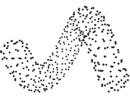
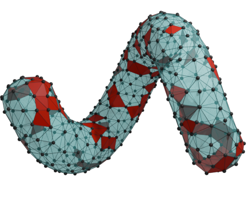
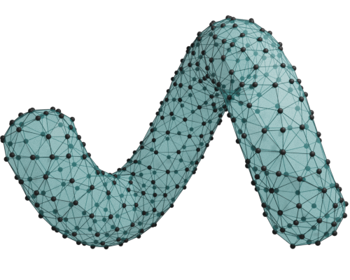
Figure 1: Points sampling a surface in $\mathbb{R}^{3}$ (a) with the corresponding $\alpha$-complex, where tetrahedra are highlighted (b). Applying Practical Squash with parameter $\alpha$ outputs (c).

   

Techniques.

Our proof of correctness for the squash algorithms is more compartmentalized than the ones present in the literature: we first consider a smooth orientable submanifold $\mathcal{M}\subseteq\mathbb{R}^{d}$ with codimension one and a general simplicial complex $K$ embedded in $\mathbb{R}^{d}$ and contained within a small tubular neighborhood of $\mathcal{M}$. We introduce vertical collapses (relative to $\mathcal{M}$) in $K$ which remove $d$-simplices of $K$ that either have no $d$-simplices of $K$ above them in directions normal to $\mathcal{M}$ or no $d$-simplices of $K$ below them in directions normal to $\mathcal{M}$. NaiveVerticalSimplification iteratively applies vertical collapses relative to $\mathcal{M}$. PracticalVerticalSimplification does not depend on knowledge of $\mathcal{M}$ and applies vertical collapses relative to a hyperplane, constructed dynamically based on the simplex currently considered for collapse.

We examine conditions for the correctness of these algorithms. Apart from the requirement that $K$ has no vertical $i$-simplices relative to $\mathcal{M}$ for $0<i<d$ and that its support projects onto $\mathcal{M}$ and fully covers it, we require the vertical convexity of $K$ relative to $\mathcal{M}$. This means that each normal line to $\mathcal{M}$ at a point $m$ (restricted to a small ball around $m$) intersects the support of $K$ in a convex set. For PracticalVerticalSimplification, an additional requirement is that the $(d-1)$-simplices of $K$ must form an angle of at most $\frac{\pi}{4}$ with $\mathcal{M}$.

Afterwards, we present $\operatorname{\tt PracticalSquash}$ and $\operatorname{\tt NaiveSquash}$, which initialize the previous algorithms with $K$ as the $\alpha$-complex of a point set $P\subseteq\mathbb{R}^{d}$ that samples $\mathcal{M}$. We show that correctness is guaranteed when the $i$-simplices in the $\alpha$-complex form small angles with $\mathcal{M}$ for $0<i<d$. We provide explicit upper bounds for these angles, expressed in terms of $\varepsilon$, $\delta$, and $\alpha$, where $\varepsilon$ and $\delta$ control the sample density and noise in $P$.

We analyze the case $d=3$ and provide numerical bounds on the ratios $\frac{\varepsilon}{\mathcal{R}}$ and $\frac{\alpha}{\mathcal{R}}$ that ensure the correctness of both squash algorithms. Instrumental to this step, we derive (1) which enables us to upper bound the angles of triangles in the $\alpha$-complex relative to the manifold and is of independent interest.

Related work.

The Squash algorithms (both practical and naive) are similar to Wrap [33, 12] in that they compute a subcomplex $K$ of the Delaunay complex of $P$ and then perform a sequence of collapses. However, the selection of $K$ and the nature of the collapses differ between the two methods: in the naive squash, definitions are relative to $\mathcal{M}$, unlike Wrap, which uses flow lines derived from $P$ to guide the collapsing sequence. This distinction allows us to address the general case first and then focus on the specific case of the $\alpha$-complex. Moreover, while we guarantee correctness for a larger interval of the ratio $\frac{\varepsilon}{\mathcal{R}}$ compared to previous literature, most existing work addresses non-uniform sampling cases, whereas our work focuses on uniform sampling.

The vertical convexity assumption, crucial for the correctness of our algorithms, has been employed in various forms to establish collapsibility of certain classes of simplicial complexes [1, 21, 11]. Similarly, bounding the angle between the manifold and the simplices used for reconstruction has been essential in prior work [24, 23, 22, 6, 10]. Our bound (1) remains true when replacing $\mathcal{R}$ with the local feature size of $a$, as explained in Appendix A. The thus modified bound improves upon the known bound [24, Lemma 3.5].

At last, for $d=3$, we show in Appendix G that the restricted Delaunay complex is generically homeomorphic to $\mathcal{M}$ for $\frac{\varepsilon}{\mathcal{R}}\leq 0.225$. In contrast, it is proven to be homeomorphic to $\mathcal{M}$ only if $\frac{\varepsilon}{\mathcal{R}}\leq 0.09$ [23, Theorem 13.16], a result based on the Topological Ball Theorem [23, Theorem 13.1]. Our proof bypasses this requirement, relying instead on $\operatorname{\tt NaiveSquash}$.

Outline.

After the preliminaries in Section 2, Section 3 defines vertically convex simplicial complexes. We introduce the concepts of upper and lower skins for these complexes and prove that both are homeomorphic to their orthogonal projection onto $\mathcal{M}$. Section 4 presents general conditions under which a simplicial complex $K$ can be transformed into a triangulation of $\mathcal{M}$ through either Naive or Practical vertical simplification. Section 5 provides conditions ensuring the topological correctness of both the naive and practical Squash algorithms and the restricted Delaunay complex. Detailed technical proofs are included in the appendices.

2 Preliminaries

Subsets and submanifold.

Given a subset $X\subseteq\mathbb{R}^{d}$, we define several important geometric concepts. The convex hull of $X$ is denoted as $\operatorname{conv}(X)$ and the affine space spanned by $X$ as $\operatorname{Aff}(X)$. The interior of $X$ is denoted as $X^{\circ}$. The relative interior of $X$, denoted as $\operatorname{relint}(X)$, represents the interior of $X$ within $\operatorname{Aff}(X)$. For any point $x$ and radius $r$, we denote the closed ball with center $x$ and radius $r$ as $B(x,r)$. The $r$-offset of $X$, denoted as $X^{\oplus r}$, is the union of closed balls centered at each point in $X$ with radius $r$: $X^{\oplus r}=\bigcup_{x\in X}B(x,r)$. The medial axis of $X$, denoted as $\operatorname{axis}(X)$, is the set of points in $\mathbb{R}^{d}$ that have at least two nearest points in $X$. The reach of $X$, denoted as $\operatorname{Reach}(X)$, is the infimum of distances between $X$ and $\operatorname{axis}(X)$. Furthermore, we define the projection map $\pi_{X}:\mathbb{R}^{d}\setminus\operatorname{axis}(X)\to X$, which associates each point $x$ with its unique closest point in $X$. This projection map is well-defined on every subset of $\mathbb{R}^{d}$ that does not intersect $\operatorname{axis}(X)$, particularly on every $r$-offset of $X$ with $r<\operatorname{Reach}(X)$.

Given $m\in\mathcal{M}$, we denote the affine tangent space to $\mathcal{M}$ at $m$ as $\mathbf{T}_{m}\mathcal{M}$ and the affine normal space as $\mathbf{N}_{m}\mathcal{M}$. As $\mathcal{M}$ has codimension one, $\mathbf{T}_{m}\mathcal{M}$ is a hyperplane and $\mathbf{N}_{m}\mathcal{M}$ is a line. Additionally, since $\mathcal{M}$ is $C^{2}$, it has a positive reach [46]. For all real numbers $r$ such that $0<r<\operatorname{Reach}(\mathcal{M})$, the $r$-offset of $\mathcal{M}$ can be partitioned into the set of normal segments $\{\mathbf{N}_{m}\mathcal{M}\cap B(m,r)\}_{m\in\mathcal{M}}$ [27], that is,

$$\mathcal{M}^{\oplus r}=\dot{\bigcup}_{m\in\mathcal{M}}\mathbf{N}_{m}\mathcal{M}\cap B(m,r).$$

Abstract simplicial complexes and collapses.

We recall some classical definitions of algebraic topology [43, 31]. An abstract simplicial complex is a collection $K$ of finite non-empty sets with the property that if $\sigma$ belongs to $K$, so does every non-empty subset of $\sigma$. Each element $\sigma$ of $K$ is called an abstract simplex and its dimension is one less than its cardinality: $\dim\sigma=\operatorname{card}\sigma-1$. A simplex of dimension $i$ is called an $i$-simplex and the set of $i$-simplices of $K$ is denoted as $K^{[i]}$. If $\tau$ and $\sigma$ are two simplices such that $\tau\subseteq\sigma$, then $\tau$ is called a face of $\sigma$, and $\sigma$ is called a coface of $\tau$. The $(d-1)$-dimensional faces of $\sigma$ are the facets of $\sigma$. The vertex set of $K$ is $\operatorname{Vert}{K}=\bigcup_{\sigma\in K}\sigma$. A subcomplex $L$ of $K$ is a simplicial complex whose elements belong to $K$. The link of $\sigma$ in $K$, denoted $\operatorname{Lk}(\sigma,K)$, is the set of simplices $\tau$ in $K$ such that $\tau\cup\sigma\in K$ and $\tau\cap\sigma=\emptyset$. It is a subcomplex of $K$. The star of $\sigma$ in $K$, denoted as $\operatorname{St}(\sigma,K)$, is the set of cofaces of $\sigma$. The simplicial complex formed by all the faces of $\sigma$ is the closure of $\sigma$, $\operatorname{Cl}\sigma$.

Consider next an abstract simplex $\sigma\subseteq\mathbb{R}^{d}$. One can associate it to the geometric simplex $\operatorname{conv}(\sigma)\subseteq\mathbb{R}^{d}$, called the support of $\sigma$. In general, $\dim(\operatorname{Aff}(\sigma))\leq\dim(\sigma)$ and we say that $\sigma$ is non-degenerate whenever $\dim(\operatorname{Aff}(\sigma))=\dim\sigma$. Given a simplicial complex $K$ with vertices in $\mathbb{R}^{d}$, we say that $K$ is canonically embedded if the following two conditions are satisfied:

1. $\dim\sigma=\dim(\operatorname{Aff}(\sigma))$ for all $\sigma\in K$;

2. $\operatorname{conv}(\alpha\cap\beta)=\operatorname{conv}(\alpha)\cap\operatorname{conv}(\beta)$ for all $\alpha,\beta\in K$.

Given such a simplicial complex, its underlying space (or support) is the point set $\boldsymbol{\lvert}K\boldsymbol{\rvert}=\bigcup_{\sigma\in K}\operatorname{conv}(\sigma)$. If $\boldsymbol{\lvert}K\boldsymbol{\rvert}$ is homeomorphic to $\mathcal{M}$, then $K$ is called a triangulation of $\mathcal{M}$ or is said to triangulate $\mathcal{M}$. Since $K$ is canonically embedded, the link of every $i$-simplex of $K$ falls into one of the following two categories: (1) it is a triangulation of the sphere of dimension $d-i-1$ or (2) it is a proper subcomplex of such a triangulation. The boundary complex of a simplicial complex $K$ is the subset of simplices in the second category, denoted $\partial K$, and it holds that $\boldsymbol{\lvert}\partial K\boldsymbol{\rvert}=\partial\boldsymbol{\lvert}K\boldsymbol{\rvert}$. Simplices in $\partial K$ are referred to as boundary simplices of $K$. Given a set of abstract simplices $\Sigma$, if $\sigma\in\Sigma$ has no coface in $\Sigma$ besides itself, then $\sigma$ is said to be inclusion-maximal in $\Sigma$.

Suppose that $\tau\in K$ is a simplex whose star in $K$ has a unique inclusion-maximal element $\sigma\neq\tau$. Then $\tau$ is said to be free in $K$. Equivalently, $\tau$ is free in $K$ if and only if the link of $\tau$ in $K$ is the closure of a simplex. Consequently, free simplices of $K$ are always boundary simplices of $K$. However, not all boundary simplices of $K$ are necessary free. There are instances where none of them are free, such as the famous example when $K$ triangulates the 2-dimensional subspace of $\mathbb{R}^{3}$, known as the “house with two rooms”. A collapse in $K$ is the operation that removes from $K$ a free simplex $\tau$ along with all its cofaces. This operation is known to preserve the homotopy-type of $\boldsymbol{\lvert}K\boldsymbol{\rvert}$.

Delaunay complexes, $\alpha$-complexes, and $\alpha$-shapes.

Consider a finite collection of points $P\subseteq\mathbb{R}^{d}$. The Voronoi region of $q\in P$ is the collection of points $x\in\mathbb{R}^{d}$ that are closer to $q$ than to any other points of $P$:

$$V(q,P)=\{x\in\mathbb{R}^{d}\mid\|x-q\|\leq\|x-p\|,\text{ for all $p\in P$}\}.$$

Given a subset $\sigma\subseteq P$, let $V(\sigma,P)=\bigcap_{q\in\sigma}V(q,P)$. The Delaunay complex is defined as

$$\operatorname{Del}(P)=\{\sigma\subseteq P\mid\sigma\neq\emptyset\text{ and }V(\sigma,P)\neq\emptyset\}.$$

A simplex $\sigma\in\operatorname{Del}(P)$ is called a Delaunay simplex of $P$ and it is dual to its corresponding Voronoi cell $V(\sigma,P)$. Henceforth, we assume that the set of points $P$ is in general position. This means that no $d+2$ points of $P$ lie on the same $d$-dimensional sphere and no $k+2$ points of $P$ lie on the same $k$-dimensional flat for $k<d$. In that case, $\operatorname{Del}(P)$ is canonically embedded [36]. For $\alpha\geq 0$, the $\alpha$-complex of $P$ is the subcomplex of $\operatorname{Del}(P)$ defined by:

$$\operatorname{Del}(P,\alpha)=\{\sigma\subseteq P\mid\sigma\neq\emptyset\text{ and }V(\sigma,P)\cap P^{\oplus\alpha}\neq\emptyset\}.$$

Its underlying space $\boldsymbol{\lvert}\operatorname{Del}(P,\alpha)\boldsymbol{\rvert}=\bigcup_{\sigma\in\operatorname{Del}(P,\alpha)}\operatorname{conv}(\sigma)$ is called the $\alpha$-shape of $P$. It has the properties: (i) $\boldsymbol{\lvert}\operatorname{Del}(P,\alpha)\boldsymbol{\rvert}\subseteq P^{\oplus\alpha}$ and (ii) $\boldsymbol{\lvert}\operatorname{Del}(P,\alpha)\boldsymbol{\rvert}$ is homotopy equivalent to $P^{\oplus\alpha}$; see [30] for more details.

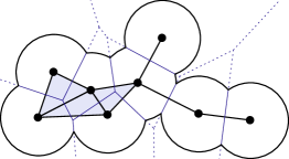
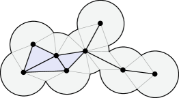
Figure 2: Left: $P$ is such that neither $P^{\oplus\alpha}$ nor $\operatorname{Del}(P,\alpha)$ are vertically convex relative to a horizontal line. Right: Decomposition of $P^{\oplus\alpha}\setminus\boldsymbol{\lvert}\operatorname{Del}(P,\alpha)\boldsymbol{\rvert}^{\circ}$ in joins as described in [30].

3 Vertically convex simplicial complexes

In this section, we define the concept of vertical convexity relative to $\mathcal{M}$ for both a set and a simplicial complex. We then study the boundary of a vertically convex simplicial complex $K$. Specifically, we divide the boundary of its underlying space into an upper and a lower skins, enabling us to identify two boundary subcomplexes: an upper and a lower ones. Furthermore, we show that each of these subcomplexes triangulates the orthogonal projection of $\boldsymbol{\lvert}K\boldsymbol{\rvert}$ onto $\mathcal{M}$ (Lemma 3.7). We also extend the definitions for a single $d$-simplex.

Definition 3.1 (Vertical convexity).

A set $X\subseteq\mathbb{R}^{d}$ is vertically convex relative to $\mathcal{M}$ if $\exists\,r\in[0,\operatorname{Reach}(\mathcal{M}))$ such that

1. $X\subseteq\mathcal{M}^{\oplus r}$ and

2. $\forall\,m\in\mathcal{M}$, $\mathbf{N}_{m}\mathcal{M}\cap B(m,r)\cap X$ is convex.

In other words, for any $m\in\mathcal{M}$, the set $\mathbf{N}_{m}\mathcal{M}\cap B(m,r)\cap X$ is either empty or a line segment (possibly of zero-length). A simplicial complex $K$ is vertically convex relative to $\mathcal{M}$ if its underlying space $\boldsymbol{\lvert}K\boldsymbol{\rvert}$ is.

Figure 3: A simplicial complex $K$ vertically convex relative to the curve $\mathcal{M}$. Each segment $\mathbf{N}_{m}\mathcal{M}\cap B(m,r)$ (in dashed orange) intersects $\boldsymbol{\lvert}K\boldsymbol{\rvert}$ in a line segment, as highlighted (blue) for the point $m$ (represented by a black square). Lemma 3.5 shows that each of the two skins of $\boldsymbol{\lvert}K\boldsymbol{\rvert}$, depicted in green and pink according to the labeling arrows, is homeomorphic to $\mathcal{M}$.

Remark 3.2.

The assumption that there exists $r<\operatorname{Reach}(\mathcal{M})$ such that $X\subseteq\mathcal{M}^{\oplus r}$ can be satisfied in practice by choosing $X$ as the $\alpha$-shape of a point set $P$ that is contained in a $\delta$-offset of $\mathcal{M}$ with $\delta+\alpha<\operatorname{Reach}(\mathcal{M})$. Indeed, setting $r=\delta+\alpha$, we have that $\boldsymbol{\lvert}\operatorname{Del}(P,\alpha)\boldsymbol{\rvert}\subseteq P^{\oplus\alpha}\subseteq\mathcal{M}^{\oplus r}$ with $r<\operatorname{Reach}(\mathcal{M})$.

Examples of a non-vertically convex and a vertically convex simplicial complexes are provided in Figures 2 and 3, respectively.

3.1 Upper and lower skins

Assume that $X\subseteq\mathbb{R}^{d}$ is vertically convex relative to $\mathcal{M}$ and let $m\in\pi_{\mathcal{M}}(X)$. The endpoints (possibly equal) of the segment $\mathbf{N}_{m}\mathcal{M}\cap B(m,r)\cap X$ are denoted by $\operatorname{low}_{X}(m)$ and $\operatorname{up}_{X}(m)$, with $\operatorname{up}_{X}(m)$ being above $\operatorname{low}_{X}(m)$ along the direction of the unit normal vector $\mathbf{n}({m})$. With this notation, $X$ can be expressed as a union of disjoint normal segments:

$$X=\dot{\bigcup}_{m\in\pi_{\mathcal{M}}(X)}[\operatorname{low}_{X}(m),\operatorname{up}_{X}(m)].$$

The upper skin and lower skin of $X$ are, respectively:

$$\operatorname{UpperSkin}_{\mathcal{M}}(X) =\{\operatorname{up}_{X}(m)\mid m\in\pi_{\mathcal{M}}(X)\},$$

$$\operatorname{LowerSkin}_{\mathcal{M}}(X) =\{\operatorname{low}_{X}(m)\mid m\in\pi_{\mathcal{M}}(X)\}.$$

Figure 3 displays an example. Our goal is to study the skins of $\boldsymbol{\lvert}K\boldsymbol{\rvert}$, for which we need two extra definitions.

Definition 3.3 (Vertical simplex).

A simplex $\sigma\subseteq\mathbb{R}^{d}$ such that $\operatorname{conv}(\sigma)\subseteq\mathbb{R}^{d}\setminus\operatorname{axis}(\mathcal{M})$ is vertical relative to $\mathcal{M}$ if there exists a pair of distinct points in $\operatorname{conv}(\sigma)$ sharing the same projection onto $\mathcal{M}$.

Definition 3.4 (Non-vertical skeleton).

Assume that $\boldsymbol{\lvert}K\boldsymbol{\rvert}\subseteq\mathbb{R}^{d}\setminus\operatorname{axis}(\mathcal{M})$. We say that $K$ has a non-vertical skeleton relative to $\mathcal{M}$ if $K$ contains no vertical $i$-simplices relative to $\mathcal{M}$ for all integers $0<i<d$.

The next lemma is a key property of vertically convex simplicial complexes:

Lemma 3.5

Suppose that $K$ is vertically convex and has a non-vertical skeleton relative to $\mathcal{M}$. Then, the upper and lower skins of $\boldsymbol{\lvert}K\boldsymbol{\rvert}$ are closed sets, each homeomorphic to $\pi_{\mathcal{M}}(\boldsymbol{\lvert}K\boldsymbol{\rvert})$. The homeomorphism is realized in both cases by $\pi_{\mathcal{M}}$. In addition,

$$\partial\boldsymbol{\lvert}K\boldsymbol{\rvert}=\operatorname{UpperSkin}_{\mathcal{M}}(\boldsymbol{\lvert}K\boldsymbol{\rvert})\cup\operatorname{LowerSkin}_{\mathcal{M}}(\boldsymbol{\lvert}K\boldsymbol{\rvert}).$$ (2)

A simple consequence follows:

Lemma 3.6.

Let $K$ be vertically convex and with non-vertical skeleton relative to $\mathcal{M}$. If $\operatorname{UpperSkin}_{\mathcal{M}}(\boldsymbol{\lvert}K\boldsymbol{\rvert})=\operatorname{LowerSkin}_{\mathcal{M}}(\boldsymbol{\lvert}K\boldsymbol{\rvert})$, then $K=\partial K$.

Aiming for a simplicial version of Equation (2), we define the upper complex of $K$ and the lower complex of $K$ relative to $\mathcal{M}$ as follows:

$$\operatorname{UpperComplex}_{\mathcal{M}}(K) =\{\nu\subseteq\partial K\mid\operatorname{conv}(\nu)\subseteq\operatorname{UpperSkin}_{\mathcal{M}}(\boldsymbol{\lvert}K\boldsymbol{\rvert})\},$$

$$\operatorname{LowerComplex}_{\mathcal{M}}(K) =\{\nu\subseteq\partial K\mid\operatorname{conv}(\nu)\subseteq\operatorname{LowerSkin}_{\mathcal{M}}(\boldsymbol{\lvert}K\boldsymbol{\rvert})\}.$$

By construction, both are subcomplexes of $\partial K$. A combinatorial equivalent of Lemma 3.5 is:

Lemma 3.7

Let $K$ be vertically convex with non-vertical skeleton relative to $\mathcal{M}$. Then,

$$\boldsymbol{\lvert}\operatorname{UpperComplex}_{\mathcal{M}}(K)\boldsymbol{\rvert}=\operatorname{UpperSkin}_{\mathcal{M}}(\boldsymbol{\lvert}K\boldsymbol{\rvert}),$$

$$\boldsymbol{\lvert}\operatorname{LowerComplex}_{\mathcal{M}}(K)\boldsymbol{\rvert}=\operatorname{LowerSkin}_{\mathcal{M}}(\boldsymbol{\lvert}K\boldsymbol{\rvert})\,\,\,\text{ and }$$

$$\partial K=\operatorname{UpperComplex}_{\mathcal{M}}(K)\,\cup\,\operatorname{LowerComplex}_{\mathcal{M}}(K).$$

Moreover, if $\pi_{\mathcal{M}}(\boldsymbol{\lvert}K\boldsymbol{\rvert})=\mathcal{M}$, both $\operatorname{UpperComplex}_{\mathcal{M}}(K)$ and $\operatorname{LowerComplex}_{\mathcal{M}}(K)$ are triangulations of $\mathcal{M}$.

3.2 Upper and lower facets of a $d$-simplex

Let $\sigma$ be a non-degenerate $d$-simplex of $\mathbb{R}^{d}$ such that $\operatorname{conv}(\sigma)\subseteq\mathcal{M}^{\oplus r}$ for some $r<\operatorname{Reach}(\mathcal{M})$. In that case, $\operatorname{Cl}\sigma$ is embedded and vertically convex relative to $\mathcal{M}$. The facets of $\sigma$ can be partitioned into upper facets and lower facets of $\sigma$ relative to $\mathcal{M}$ as follows:

$$\operatorname{UpperFacets}_{\mathcal{M}}(\sigma) =\{\nu\text{ facet of }\sigma\mid\nu\in\operatorname{UpperComplex}_{\mathcal{M}}(\operatorname{Cl}\sigma)\}$$

$$\operatorname{LowerFacets}_{\mathcal{M}}(\sigma) =\{\nu\text{ facet of }\sigma\mid\nu\in\operatorname{LowerComplex}_{\mathcal{M}}(\operatorname{Cl}\sigma)\}.$$

An example can be seen in Figure 4, where one can also observe the following property:

Figure 4: Upper (smooth green edges) and lower (dotted pink edge) facets of a $2$-simplex $\sigma\subseteq\mathbb{R}^{2}$.

Lemma 3.8

Consider a non-degenerate $d$-simplex $\sigma\subseteq\mathbb{R}^{d}$ such that $\operatorname{conv}(\sigma)\subseteq\mathcal{M}^{\oplus r}$ for some $r<\operatorname{Reach}(\mathcal{M})$. If $\sigma$ has no vertical facets relative to $\mathcal{M}$, then $\operatorname{UpperFacets}_{\mathcal{M}}(\sigma)$ and $\operatorname{LowerFacets}_{\mathcal{M}}(\sigma)$ are non-empty sets that partition the facets of $\sigma$.

4 Vertically collapsing simplicial complexes

In this section, assuming that $\boldsymbol{\lvert}K\boldsymbol{\rvert}\subseteq\mathcal{M}^{\oplus r}$ for some $r<\operatorname{Reach}(\mathcal{M})$, we introduce an algorithm for simplifying $K$ using vertical collapses relative to $\mathcal{M}$ (Section 4.1) and establish conditions for when it outputs a triangulation of $\mathcal{M}$ (Section 4.2). We first present a naive version that requires the knowledge of $\mathcal{M}$ and then present a practical version (Section 4.3).

4.1 Naive algorithm

Definition 4.1 (Vertically free simplices).

A simplex $\tau$ is said to be free from above (resp., free from below) in $K$ relative to $\mathcal{M}$ if

• $\tau$ is a free simplex of $K$;

• the unique inclusion-maximal simplex $\sigma$ in $\operatorname{St}(\tau,K)$ has dimension $d$;

• the set of $(d-1)$-simplices in $\operatorname{St}(\tau,K)$ is exactly the set of upper (resp., lower) facets of $\sigma$ relative to $\mathcal{M}$.

We say that $\tau$ is vertically free in $K$ relative to $\mathcal{M}$ if $\tau$ is either free from above or from below in $K$ relative to $\mathcal{M}$.

See Figures 5 and 7 for a depiction. Note that the definition can be naturally extended to non-compact $\mathcal{M}$. In particular, it holds for hyperplanes, a fact that we use in Algorithm 2.

Definition 4.2 (Vertical collapse).

A vertical collapse of $K$ relative to $\mathcal{M}$ is the operation of removing the star of a simplex $\tau\in K$ that is vertically free relative to $\mathcal{M}$.

Figure 5: Schematic drawings of $K$ in blue (smooth filled areas). Top row: the edge $\tau$ is free but not vertically free relative to $\mathcal{M}$ and collapsing $\tau$ does not preserve the vertical convexity of $K$. Bottom row: the vertex $\tau$ is free from above relative to $\mathcal{M}$, so that collapsing $\tau$ preserves the vertical convexity of $K$ (Lemma 4.6). The $(d-1)$-simplices of $K$ that disappear with $\tau$ are precisely the upper facets of $\sigma$ (smooth edges, in green).

A vertical collapse of $K$ can be seen as compressing the underlying space of $K$ by shifting its upper or lower skin along directions normal to $\mathcal{M}$; see Figure 5. Our first algorithm, outlined in Algorithm 1, simplifies $K$ by iteratively applying vertical collapses relative to $\mathcal{M}$. It is worth noting that the algorithm operates on any simplicial complex $K$ with $\boldsymbol{\lvert}K\boldsymbol{\rvert}\subseteq\mathcal{M}^{\oplus r}$ for $r<\operatorname{Reach}(\mathcal{M})$, irrespective of whether $K$ is vertically convex relative to $\mathcal{M}$ or not.

Algorithm 1 $\hyperlink{naivealgo}{\operatorname{\tt NaiveVerticalSimplification}}(K)$

  while  there is a simplex $\tau$ vertically free in $K$ relative to $\mathcal{M}$ do

      Collapse $\tau$ in $K$;

  end while

4.2 Correctness

We now establish conditions under which $\hyperlink{naivealgo}{\operatorname{\tt NaiveVerticalSimplification}}(K)$ transforms $K$ into a triangulation of $\mathcal{M}$. For that, we introduce a binary relation over $d$-simplices:

Definition 4.3 (Below relation $\prec_{\mathcal{M}}$).

Let $\sigma_{0},\sigma_{1}\subseteq\mathbb{R}^{d}$ be two $d$-simplices sharing a common facet $\nu=\sigma_{0}\cap\sigma_{1}$ and let $\operatorname{conv}(\sigma_{0})\cup\operatorname{conv}(\sigma_{1})\subseteq\mathcal{M}^{\oplus r}$ for some $r<\operatorname{Reach}(\mathcal{M})$. We say that $\sigma_{0}$ is below $\sigma_{1}$ (or that $\sigma_{1}$ is above $\sigma_{0}$) relative to $\mathcal{M}$, denoted $\sigma_{0}\prec_{\mathcal{M}}\sigma_{1}$, if $\nu$ is an upper facet of $\sigma_{0}$ and a lower facet of $\sigma_{1}$ relative to $\mathcal{M}$.

Note that the relation $\prec_{\mathcal{M}}$ is not acyclic in general, see Figure 6.

Figure 6: Non-Delaunay triangles that form a cycle in the $\prec_{\mathcal{M}}$ relation and their dual graph.

Theorem 4.4 (Correctness).

Consider $K$ such that $\boldsymbol{\lvert}K\boldsymbol{\rvert}\subseteq\mathcal{M}^{\oplus r}$ for some $r<\operatorname{Reach}(\mathcal{M})$ and assume the following:

Injective projection:

$K$ has a non-vertical skeleton relative to $\mathcal{M}$.

Covering projection:

$\pi_{\mathcal{M}}(\boldsymbol{\lvert}K\boldsymbol{\rvert})=\mathcal{M}$.

Vertical convexity:

$K$ is vertically convex relative to $\mathcal{M}$.

Acyclicity:

$\prec_{\mathcal{M}}$ is acyclic over $d$-simplices of $K$.

Then, $\hyperlink{naivealgo}{\operatorname{\tt NaiveVerticalSimplification}}(K)$ transforms $K$ into a triangulation of $\mathcal{M}$.

The remaining of this section aims to prove Theorem 4.4 and we consider $K$ such that $\boldsymbol{\lvert}K\boldsymbol{\rvert}\subseteq\mathcal{M}^{\oplus r}$ for some $r<\operatorname{Reach}(\mathcal{M})$. Using the relation $\prec_{\mathcal{M}}$, associate to $K$ its dual graph $G_{\mathcal{M}}(K)$ that has one node for each $d$-simplex of $K$ and one arc for each pair of $d$-simplices $\sigma_{0},\sigma_{1}\in K$ that share a common facet $\sigma_{0}\cap\sigma_{1}$. Direct an arc from $\sigma_{0}$ to $\sigma_{1}$ if $\sigma_{0}\prec_{\mathcal{M}}\sigma_{1}$, and from $\sigma_{1}$ to $\sigma_{0}$ otherwise. Since either $\sigma_{0}\prec_{\mathcal{M}}\sigma_{1}$ or $\sigma_{1}\prec_{\mathcal{M}}\sigma_{0}$, this yields a well-defined orientation for each arc in the dual graph. Figures 6 and 7 show examples.

Figure 7: A vertically convex simplicial complex $K$ relative to $\mathcal{M}$. All free simplices are highlighted by thickness. There are four simplices free from below (represented by three dotted edges and one triangular vertex, in pink) and four simplices free from above (represented by two dashed edges and two square vertices, in green). The dual graph (oriented edges, in blue) has four sources (vertices filled by dots, in pink) and four sinks (vertices with a smooth filling, in green), in one-to-one correspondence with the free simplices from below and above.

In a directed graph, a source is a node with only outgoing arcs, while a sink is a node with only incoming arcs. The next lemma states that a vertical collapse in $K$ corresponds to the removal of either a sink or a source in $G_{\mathcal{M}}(K)$ and conversely. For that, given a finite set of abstract simplices $\Sigma=\{\sigma_{1},\sigma_{2},\ldots,\sigma_{k}\}$, let $\bigcap\Sigma=\bigcap_{i=1}^{k}\sigma_{i}$ denote the set of vertices that belong to all simplices in $\Sigma$. If $\bigcap\Sigma\neq\emptyset$, it forms an abstract simplex.

Lemma 4.5 (Sinks and sources)

Consider $K$ such that $\boldsymbol{\lvert}K\boldsymbol{\rvert}\subseteq\mathcal{M}^{\oplus r}$ for some $r<\operatorname{Reach}(\mathcal{M})$ and assume that $K$ satisfies the injective projection, covering projection and vertical convexity assumptions of Theorem 4.4. Consider a $d$-simplex $\sigma\in K$ and let $\tau=\bigcap{\operatorname{UpperFacets}_{\mathcal{M}}(\sigma)}$ and $\tau^{\prime}=\bigcap{\operatorname{LowerFacets}_{\mathcal{M}}(\sigma)}$. Then,

• $\tau$ is a free simplex of $K$ from above relative to $\mathcal{M}$ $\iff$ $\sigma$ is a sink of $G_{\mathcal{M}}(K)$.

• $\tau^{\prime}$ is a free simplex of $K$ from below relative to $\mathcal{M}$ $\iff$ $\sigma$ is a source of $G_{\mathcal{M}}(K)$.

The next lemma provides an invariant for the while-loop of Algorithm 1.

Lemma 4.6 (Loop invariant).

Consider $K$ such that $\boldsymbol{\lvert}K\boldsymbol{\rvert}\subseteq\mathcal{M}^{\oplus r}$ for some $r<\operatorname{Reach}(\mathcal{M})$. Let $\tau$ be a vertically free simplex in $K$ relative to $\mathcal{M}$. Let $K^{\prime}$ be obtained from $K$ by collapsing $\tau$ in $K$. If $K$ satisfies the assumptions of Theorem 4.4, then so does $K^{\prime}$.

Proof 4.7 (Proof of Theorem 4.4.).

Since $K$ is vertically convex relative to $\mathcal{M}$ and $\pi_{\mathcal{M}}(\boldsymbol{\lvert}K\boldsymbol{\rvert})=\mathcal{M}$, the set $\mathbf{N}_{m}\mathcal{M}\cap B(m,r)\cap\boldsymbol{\lvert}K\boldsymbol{\rvert}$ forms a segment for all $m\in\mathcal{M}$. The endpoints of this segment are denoted $\operatorname{low}_{K}(m)$ and $\operatorname{up}_{K}(m)$. First, we show that for all $m\in\mathcal{M}$, if $\operatorname{low}_{K}(m)\neq\operatorname{up}_{K}(m)$, then the segment $[\operatorname{low}_{K}(m),\operatorname{up}_{K}(m)]$ intersects the support of at least one $d$-simplex of $K$, implying $G_{\mathcal{M}}(K)\neq\emptyset$. Suppose, for a contradiction, that $[\operatorname{low}_{K}(m),\operatorname{up}_{K}(m)]$ only intersects the support of $i$-simplices of $K$ for $i<d$. As $\operatorname{low}_{K}(m)\neq\operatorname{up}_{K}(m)$ and $K$ has a finite number of simplices, at least one of these $i$-simplices, say $\nu$, intersects $[\operatorname{low}_{K}(m),\operatorname{up}_{K}(m)]$ in a non-zero length segment containing distinct points $x,y\in\operatorname{conv}(\nu)\cap[\operatorname{low}_{K}(m),\operatorname{up}_{K}(m)]$. Hence, $x$ and $y$ share the same orthogonal projection $m$ onto $\mathcal{M}$, implying that $\nu$ is vertical relative to $\mathcal{M}$. This contradicts the injective projection assumption on $K$. Thus,

$$\exists m\in\mathcal{M},\;\operatorname{low}_{K}(m)\neq\operatorname{up}_{K}(m)\quad\implies\quad G_{\mathcal{M}}(K)\neq\emptyset.$$ (3)

We now prove the correctness of $\hyperlink{naivealgo}{\operatorname{\tt NaiveVerticalSimplification}}(K)$. The algorithm starts with $K$ that satisfies the theorem assumptions and by Lemma 4.6, after each iteration of the while-loop we obtain a new $K$ that continues to satisfy those assumptions. Since each iteration involves a vertical collapse of $K$ relative to $\mathcal{M}$, the number of $d$-simplices of $K$ is reduced. Thus, the algorithm must terminate. Upon termination, there are no vertically free simplices in $K$ relative to $\mathcal{M}$. By Lemma 4.5, this implies that $G_{\mathcal{M}}(K)$ has no terminal node (neither a source nor a sink) and is therefore empty. The contrapositive of (3) yields that for all $m\in\mathcal{M}$, $\operatorname{low}_{K}(m)=\operatorname{up}_{K}(m)$. In other words, when Algorithm 1 terminates, $\operatorname{LowerSkin}_{\mathcal{M}}(K)=\operatorname{UpperSkin}_{\mathcal{M}}(K)$. By Lemma 3.6, we have $K=\partial K$ and Lemma 3.7 implies

$$K=\partial K=\operatorname{UpperComplex}_{\mathcal{M}}(K)=\operatorname{LowerComplex}_{\mathcal{M}}(K),$$

with $K$ being a triangulation of $\mathcal{M}$.

4.3 Practical version

Algorithm 1 relies on knowledge of $\mathcal{M}$, which renders it impractical for implementation since $\mathcal{M}$ is typically unknown. In this section, we introduce Algorithm 2, a feasible variant that is correct if the $(d-1)$-simplices of $K$ form a sufficiently small angle with $\mathcal{M}$; see Appendix A for a definition of the angle between affine spaces. In this variant, we assign an affine space $\mathcal{H}_{\tau}$ to each $\tau\in K$: for a free simplex $\tau$ with a $d$-dimensional coface $\sigma$, $\mathcal{H}_{\tau}$ is defined as the hyperplane spanned by any facet of $\sigma$. Otherwise, set $\mathcal{H}_{\tau}=\emptyset$.

Algorithm 2 $\hyperlink{practicalalgo}{\operatorname{\tt PracticalVerticalSimplification}}(K)$

  while  there is a simplex $\tau$ vertically free in $K$ relative to $\mathcal{H}_{\tau}$  do

      Collapse $\tau$ in $K$;

  end while

Theorem 4.8 (Correctness).

Suppose that $K$ satisfies the assumptions of Theorem 4.4 and, in addition, for all $(d-1)$-simplices $\nu$ of $K$

$$\max_{a\in\nu}\angle(\operatorname{Aff}(\nu),\mathbf{T}_{\pi_{\mathcal{M}}(a)}\mathcal{M})\,<\,\frac{\pi}{4}.$$ (4)

Then, $\hyperlink{practicalalgo}{\operatorname{\tt PracticalVerticalSimplification}}(K)$ transforms $K$ into a triangulation of $\mathcal{M}$.

5 Correct reconstructions from $\alpha$-complexes

In this section, we assume that $\mathcal{M}$ is sampled by a finite point set $P$ and consider Algorithms 3 and 4, which apply vertical collapses to $\operatorname{Del}(P,\alpha)$ either straightforwardly or practically. We introduce two parameters, $\varepsilon\geq 0$ and $\delta\geq 0$, to control the sample density and noise of $P$, respectively, and a scale parameter $\alpha\geq 0$. Section 5.1 establishes conditions ensuring the correctness of Algorithms 3 and 4, with the proof outlined in Section 5.2. Section 5.3 shows how these conditions hold for a wide range of $\frac{\varepsilon}{\mathcal{R}}$ and $\frac{\alpha}{\mathcal{R}}$ when $\mathcal{M}$ is a surface in $\mathbb{R}^{3}$ and $P$ is noiseless. This result is extended to the restricted Delaunay complex of $P$ in Section 5.4.

Algorithm 3 $\operatorname{\tt NaiveSquash}(P,\alpha)$

   $K\leftarrow\operatorname{Del}(P,\alpha)$; $\hyperlink{naivealgo}{\operatorname{\tt NaiveVerticalSimplification}}(K)$; return $K$;

Algorithm 4 $\operatorname{\tt PracticalSquash}(P,\alpha)$

   $K\leftarrow\operatorname{Del}(P,\alpha)$; $\hyperlink{practicalalgo}{\operatorname{\tt PracticalVerticalSimplification}}(K)$; return $K$;

5.1 Sampling and angular conditions in $\mathbb{R}^{d}$

The next definition enables us to express our results in $\mathbb{R}^{d}$ more concisely.

Definition 5.1 (Strict homotopy condition).

We say that $\varepsilon,\delta\geq 0$ satisfy the strict homotopy condition if $(\mathcal{R}-\delta)^{2}-\varepsilon^{2}>(4\sqrt{2}-5)\mathcal{R}^{2}$ for $\delta\leq\varepsilon$ and $\varepsilon+\sqrt{2}\delta<(\sqrt{2}-1)\mathcal{R}$ for $\delta\geq\varepsilon$.

Let $I(\varepsilon,\delta)$ be an interval of $\alpha$ values so that $P^{\oplus\alpha}$ is vertically convex with relation to $\mathcal{M}$. The exact definition can be found in Appendix D.1. The fact that this interval guarantees vertical convexity follows from the specialization of Propositions $5$ and $7$ in [7] to the case where $\mathcal{M}$ has codimension-one:

Theorem 5.2 (Specialization of [7]).

Suppose that $\mathcal{M}\subseteq P^{\oplus\varepsilon}$ and $P\subseteq\mathcal{M}^{\oplus\delta}$ with $\varepsilon,\delta\geq 0$ that satisfy the strict homotopy condition. Then, for all $\alpha\in I(\varepsilon,\delta)$, $\pi_{\mathcal{M}}(P^{\oplus\alpha})=\mathcal{M}$ and $P^{\oplus\alpha}$ is vertically convex relative to $\mathcal{M}$. Thus, $P^{\oplus\alpha}$ has associated upper and lower skins and deformation-retracts onto $\mathcal{M}$ along $\pi_{\mathcal{M}}$. In addition, the two skins partition $\partial P^{\oplus\alpha}$.

The above concepts can be put together to state our main theorem:

Theorem 5.3.

Assume $\mathcal{M}\subseteq P^{\oplus\varepsilon}$ and $P\subseteq\mathcal{M}^{\oplus\delta}$ for $\varepsilon,\delta\geq 0$ that satisfy the strict homotopy condition. Let $\alpha\in\left[\delta,\frac{2(\mathcal{R}-\delta)}{3}\right)\cap I(\varepsilon,\delta)$ and $\beta>0$ such that $\mathcal{M}^{\oplus\beta}\subseteq P^{\oplus\alpha}$. Suppose that for all $i$-simplices $\tau\in\operatorname{Del}(P,\alpha)$, $0<i<d$ and all $(d-1)$-simplices $\nu\in\operatorname{Del}(P,\alpha)$ it holds:

$$\max_{x\in\operatorname{conv}(\tau)}\angle(\operatorname{Aff}(\tau),\mathbf{T}_{\pi_{\mathcal{M}}(x)}\mathcal{M})\, <\,\frac{\pi}{2},$$ (5)

$$\min_{a\in\tau}\angle(\operatorname{Aff}(\tau),\mathbf{T}_{\pi_{\mathcal{M}}(a)}\mathcal{M})\, <\,\arcsin\left(\frac{(\mathcal{R}+\beta)^{2}-(\mathcal{R}+\delta)^{2}-\alpha^{2}}{2(\mathcal{R}+\delta)\alpha}\right)\,\text{and}$$ (6)

$$\min_{x\in\operatorname{conv}(\nu)}\angle(\operatorname{Aff}(\nu),\mathbf{T}_{\pi_{\mathcal{M}}(x)}\mathcal{M})\, <\,\frac{\pi}{2}-2\arcsin\left(\frac{\alpha}{2(\mathcal{R}-\delta-\alpha)}\right).$$ (7)

Then, $\operatorname{Del}(P,\alpha)$ satisfies the injective projection, covering projection, vertical convexity and acyclicity assumptions of Theorem 4.4. Furthermore, both the upper and lower complexes of $\operatorname{Del}(P,\alpha)$ relative to $\mathcal{M}$ are triangulations of $\mathcal{M}$ and $\operatorname{\tt NaiveSquash}(P,\alpha)$ returns a triangulation of $\mathcal{M}$.

One can check that Conditions (5), (6) and (7) are well-defined; see Remark E1.

Corollary 5.4.

Suppose the assumptions of Theorem 5.3 are satisfied and furthermore that for all $(d-1)$-simplices $\nu\in\operatorname{Del}(P,\alpha)$,

$$\max_{a\in\nu}\angle(\operatorname{Aff}(\nu),\mathbf{T}_{\pi_{\mathcal{M}}(a)}\mathcal{M})\,<\,\frac{\pi}{4}.$$ (8)

Then, $\operatorname{\tt PracticalSquash}(P,\alpha)$ returns a triangulation of $\mathcal{M}$.

5.2 Partial proof technique for Theorem 5.3

In this section, we provide an overview of how to establish the covering projection and vertical convexity of $\operatorname{Del}(P,\alpha)$ as guaranteed by Theorem 5.3. The complete proof of that theorem, which is unfortunately too lengthy to include here, can be found in Appendix E.

Lemma 5.5.

Assume $\mathcal{M}\subseteq P^{\oplus\varepsilon}$ and $P\subseteq\mathcal{M}^{\oplus\delta}$ for $\varepsilon,\delta\geq 0$ that satisfy the strict homotopy condition. Let $\alpha\in[\delta,\mathcal{R}-\delta)\cap I{(\varepsilon,\delta)}$ and $\beta>0$ be such that $\mathcal{M}^{\oplus\beta}\subseteq P^{\oplus\alpha}$. Suppose that for all $i$-simplices $\tau\in\operatorname{Del}(P,\alpha)$ with $0<i<d$, Conditions (5) and (6) hold. Then, $\pi_{\mathcal{M}}(\boldsymbol{\lvert}\operatorname{Del}(P,\alpha)\boldsymbol{\rvert})=\mathcal{M}$ and $\operatorname{Del}(P,\alpha)$ is vertically convex relative to $\mathcal{M}$.

Figure 8: Decomposing $P^{\oplus\alpha}\setminus\boldsymbol{\lvert}\operatorname{Del}(P,\alpha)\boldsymbol{\rvert}^{\circ}$ into upper joins (hashed, in green) and lower joins (dotted, in pink).

Upper and lower joins.

For proving this lemma, we introduce upper and lower joins. Consider $\mathcal{M}$, $P$, $\varepsilon$, $\delta$, $\alpha$ and $\beta$ that satisfy the assumptions of Lemma 5.5 and notice that they also meet the conditions of Theorem 5.2. Therefore, $P^{\oplus\alpha}$ has associated upper and lower skins and the two skins form a partition of $\partial P^{\oplus\alpha}$. Using that partition, we decompose the set difference $P^{\oplus\alpha}\setminus\boldsymbol{\lvert}\operatorname{Del}(P,\alpha)\boldsymbol{\rvert}^{\circ}$ into upper and lower joins, slightly adapting what is done in [30]; see Figures 2 and 8. For that, notice that $\partial P^{\oplus\alpha}$ can be decomposed into faces, each face being the restriction of $\partial P^{\oplus\alpha}$ to a Voronoi cell of $P$. There is a one-to-one correspondence between simplices of $\partial\operatorname{Del}(P,\alpha)$ and faces of $\partial P^{\oplus\alpha}$: the simplex $\tau\in\partial\operatorname{Del}(P,\alpha)$ corresponds to the face $F_{\tau}=V(\tau,P)\cap\partial P^{\oplus\alpha}$ and conversely. We can further partition each face $F_{\tau}$ of $\partial P^{\oplus\alpha}$ into a portion $F_{\tau}^{+}$ that lies on the upper skin of $\partial P^{\oplus\alpha}$ and a portion $F_{\tau}^{-}$ that lies on the lower skin of $\partial P^{\oplus\alpha}$. Note that $F_{\tau}^{+}$ or $F_{\tau}^{-}$ can be empty. We refer to $F_{\tau}^{+}$ as an upper face and $F_{\tau}^{-}$ as a lower face. The set of upper faces decompose the upper skin, while the set of lower faces decompose the lower skin. A join $X*Y$ is defined as the set of segments $[x,y]$ where $x\in X$ and $y\in Y$ [30]. We call $F_{\tau}^{+}*\operatorname{conv}(\tau)$ an upper join and $F_{\tau}^{-}*\operatorname{conv}(\tau)$ a lower join. The next lemma, proved in Appendix E.2, identifies points in $\partial|\operatorname{Del}(P,\alpha)|$ that are connected to upper or lower joins.

Remark 5.6.

The collection of upper and lower joins cover the set $P^{\oplus\alpha}\setminus\boldsymbol{\lvert}\operatorname{Del}(P,\alpha)\boldsymbol{\rvert}^{\circ}$.

Remark 5.7.

If an upper join and a lower join have a non-empty intersection, the common intersection belongs to $\boldsymbol{\lvert}\operatorname{Del}(P,\alpha)\boldsymbol{\rvert}$.

Lemma 5.8.

Under the assumptions of Lemma 5.5, let $\gamma\in\operatorname{Del}(P,\alpha)$ and $x\in\operatorname{relint}(\operatorname{conv}(\gamma))$. If for some $\lambda>0$ (resp. $\lambda<0$), the segment $(x,x+\lambda\mathbf{n}({\pi_{\mathcal{M}}(x)})]$ lies outside $\boldsymbol{\lvert}\operatorname{Del}(P,\alpha)\boldsymbol{\rvert}$, then it intersects an upper (resp. lower join).

Proof 5.9 (Proof of Lemma 5.5).

Consider $\mathcal{M}$, $P$, $\varepsilon$, $\delta$, $\alpha$ and $\beta$ that satisfy the assumptions of Lemma 5.5. As noted before, they also meet the conditions of Theorem 5.2. Therefore, $\pi_{\mathcal{M}}(P^{\oplus\alpha})=\mathcal{M}$ and $P^{\oplus\alpha}$ is vertically convex relative to $\mathcal{M}$. Hence, there exists $r<\operatorname{Reach}(\mathcal{M})$ such that $P^{\oplus\alpha}\subseteq\mathcal{M}^{\oplus r}$ and $P^{\oplus\alpha}\cap\mathbf{N}_{m}\mathcal{M}\cap B(m,r)$ is a line segment for any $m\in\mathcal{M}$. Fix $m\in\mathcal{M}$ arbitrarily. We show that $\boldsymbol{\lvert}\operatorname{Del}(P,\alpha)\boldsymbol{\rvert}\cap\mathbf{N}_{m}\mathcal{M}\cap B(m,r)$ is also a line segment.

First, let us establish that it is non empty. Let $u^{+}$ (resp. $u^{-}$) be the endpoint of the segment $P^{\oplus\alpha}\cap\mathbf{N}_{m}\mathcal{M}\cap B(m,r)$ that lies on the upper (resp. lower) skin of $P^{\oplus\alpha}$ and hence is contained in an upper (resp. lower) join. By Remark 5.6, the entire segment $[u^{+},u^{-}]$ is covered by upper and lower joins. Thus, at some point $c$ of $[u^{+},u^{-}]$, an upper join and a lower join intersect. By Remark 5.7, such an intersection places $c$ on $\boldsymbol{\lvert}\operatorname{Del}(P,\alpha)\boldsymbol{\rvert}$ as well.

Figure 9: Reaching a contradiction in the proof of Lemma 5.5. We see the simplices of $\operatorname{Del}(P,\alpha)$ whose support intersects $\mathbf{N}_{m}\mathcal{M}\cap B(m,r)$ (smooth filling, in pale blue) and one upper (hashed, in green) and one lower (dotted, in pink) joins that intersect $[a,b]$.

Second, we show by contradiction that $\boldsymbol{\lvert}\operatorname{Del}(P,\alpha)\boldsymbol{\rvert}\cap\mathbf{N}_{m}\mathcal{M}\cap B(m,r)$ is connected. Suppose that $a,b\in\boldsymbol{\lvert}\operatorname{Del}(P,\alpha)\boldsymbol{\rvert}\cap\mathbf{N}_{m}\mathcal{M}\cap B(m,r)$ are such that $[a,b]\cap\boldsymbol{\lvert}\operatorname{Del}(P,\alpha)\boldsymbol{\rvert}=\{a,b\}$ with $a$ being above $b$ along the direction of $\mathbf{n}({m})$. Since $a,b\in\boldsymbol{\lvert}\operatorname{Del}(P,\alpha)\boldsymbol{\rvert}\subseteq P^{\oplus\alpha}$ and $P^{\oplus\alpha}$ is vertically convex, the segment $[a,b]$ is contained in $P^{\oplus\alpha}$. By Remark 5.6, the entire segment $[a,b]$ is covered by upper and lower joins. Let $\gamma_{a}$ and $\gamma_{b}$ be the simplices of $\operatorname{Del}(P,\alpha)$ that contain $a$ and $b$, respectively, in their relative interior. Letting $\lambda=\frac{\|a-b\|}{2}$, then both segments $\left(a,a-\lambda\mathbf{n}({m})\right]$ and $\left(b,b+\lambda\mathbf{n}({m})\right]$ lie outside $\boldsymbol{\lvert}\operatorname{Del}(P,\alpha)\boldsymbol{\rvert}$. It follows, by Lemma 5.8, that there are at least one lower and one upper joins among the joins that cover $(a,b)$; see Figure 9. Hence, an upper and a lower joins intersect at a point $c$ of the segment $(a,b)$. By Remark 5.7, $c$ lies in $\boldsymbol{\lvert}\operatorname{Del}(P,\alpha)\boldsymbol{\rvert}$, a contradiction. Therefore, for all $m\in\mathcal{M}$, $\boldsymbol{\lvert}\operatorname{Del}(P,\alpha)\boldsymbol{\rvert}\cap\mathbf{N}_{m}\mathcal{M}\cap B(m,r)$ is non-empty and connected, thus forming a line segment.

5.3 Sampling conditions for surfaces in $\mathbb{R}^{3}$.

Theorem 5.3 requires that the $i$-simplices of $\operatorname{Del}(P,\alpha)$ form a small angle with the manifold $\mathcal{M}$, for $0<i<d$. Ensuring this can be challenging in practice, especially for $i\geq 3$. However, in the specific case of noiseless edges ($i=1$) or triangles ($i=2$), it is possible to upper bound the angle these simplices form with $\mathcal{M}$. For edges, it is known that:

Lemma 5.10 ([15, Lemma 7.8]).

If $ab$ is a non-degenerate edge with $a,b\in\mathcal{M}$, then

$$\sin\angle\operatorname{Aff}(ab),\mathbf{T}_{a}\mathcal{M}\,\leq\,\frac{\|b-a\|}{2\,\mathcal{R}}.$$

For triangles, let $\rho({\tau})$ be the radius of the smallest $(d-1)$-sphere circumscribing $\tau$. We establish a simple bound that is tighter than the previous one (see [24, Lemma 3.5]):

Lemma 5.11.

If $abc$ is a non-degenerate triangle with longest edge $bc$, for $a,b,c\in\mathcal{M}$, then

$$\sin\angle\operatorname{Aff}(abc),\mathbf{T}_{a}\mathcal{M}\, \leq\,\frac{\rho({abc})}{\mathcal{R}} abc$$ if is an obtuse triangle and

$$\sin\angle\operatorname{Aff}(abc),\mathbf{T}_{a}\mathcal{M}\, \leq\,\frac{\sqrt{3}\,\rho({abc})}{\mathcal{R}} abc$$ if is an acute triangle.

If $abc$ is obtuse, the bound is tight and happens when $\mathcal{M}$ is a sphere of radius $\mathcal{R}$.

The proof is technical and is therefore provided in Appendix A. For the same reason, Appendix F includes the proof of the following result, where we use the bounds for edges and triangles to establish sampling conditions for surfaces in $\mathbb{R}^{3}$. Let us define

$$\beta_{\varepsilon,\alpha}=-\frac{\varepsilon^{2}}{2\mathcal{R}}+\sqrt{\alpha^{2}+\frac{\varepsilon^{4}}{4\mathcal{R}^{2}}-\varepsilon^{2}},$$

which is one particular value of $\beta$ that guarantees $\mathcal{M}^{\oplus\beta}\subseteq P^{\oplus\alpha}$; see Appendix D.2.

Theorem 5.12.

Let $\mathcal{M}$ be a $C^{2}$ surface in $\mathbb{R}^{3}$ whose reach is at least $\mathcal{R}>0$. Let $P$ be a finite point set such that $P\subseteq\mathcal{M}\subseteq P^{\oplus\varepsilon}$.

1. For all $\varepsilon,\alpha\geq 0$ that satisfy $\frac{\sqrt{3}\,\alpha}{\mathcal{R}}<\min\left\{\frac{(\mathcal{R}+\beta_{\varepsilon,\alpha})^{2}-\mathcal{R}^{2}-\alpha^{2}}{2\mathcal{R}\alpha},\,\cos\left(2\arcsin\left(\frac{\alpha}{\mathcal{R}}\right)\right)\right\}$,

   • the upper and lower complexes of $\operatorname{Del}(P,\alpha)$ relative to $\mathcal{M}$ are triangulations of $\mathcal{M}$;

   • $\operatorname{\tt NaiveSquash}(P,\alpha)$ returns a triangulation of $\mathcal{M}$.

2. For all $\varepsilon,\alpha\geq 0$ that satisfy in addition $\frac{\sqrt{3}\,\alpha}{\mathcal{R}}<\sin\left(\frac{\pi}{4}-2\arcsin\left(\frac{\alpha}{\mathcal{R}}\right)\right)$,

   • $\operatorname{\tt PracticalSquash}(P,\alpha)$ returns a triangulation of $\mathcal{M}$.

The pairs of $(\frac{\varepsilon}{\mathcal{R}},\frac{\alpha}{\mathcal{R}})$ that satisfy 1 and 2 are depicted in Figures 10(a) and 10(b), respectively.

Remark 5.13.

In particular, 1 holds for $\frac{\varepsilon}{\mathcal{R}}\leq 0.225$ and $\frac{\alpha}{\mathcal{R}}=0.359$; and 2 for $\frac{\varepsilon}{\mathcal{R}}\leq 0.178$ and $\frac{\alpha}{\mathcal{R}}=0.207$, better bounds than the previous existing ones [23, Theorem 13.16][25].

(a)

(b)

Figure 10: Pairs of $(\frac{\varepsilon}{\mathcal{R}},\frac{\alpha}{\mathcal{R}})$ for which $\operatorname{\tt NaiveSquash}(P,\alpha)$ (a) and $\operatorname{\tt PracticalSquash}(P,\alpha)$ (b) are correct, for $P\subseteq\mathcal{M}\subseteq P^{\oplus\varepsilon}$ and $d=3$.

       

5.4 The restricted Delaunay complex

We recall from [34] that the restricted Delaunay complex is

$$\operatorname{Del}_{\mathcal{M}}(P)=\{\sigma\subseteq P\mid\sigma\neq\emptyset\text{ and }V(\sigma,P)\cap\mathcal{M}\neq\emptyset\}.$$

Theorem 5.14.

Let $\mathcal{M}$ be a $C^{2}$ surface in $\mathbb{R}^{3}$ whose reach is at least $\mathcal{R}>0$. Let $P$ be a finite set such that $P\subseteq\mathcal{M}\subseteq P^{\oplus\varepsilon}$ for $0\leq\frac{\varepsilon}{\mathcal{R}}\leq 0.225$. Under the additional generic assumption that all Voronoi cells of $P$ intersect $\mathcal{M}$ transversally, $\operatorname{Del}_{\mathcal{M}}(P)$ is a triangulation of $\mathcal{M}$.

Contents

[1]APPENDIX CONTENTS

.tocmtappendix mtchapternone mtappendixsubsection

Contents

1. 1 Introduction
2. 2 Preliminaries
3. 3 Vertically convex simplicial complexes
   1. 3.1 Upper and lower skins
   2. 3.2 Upper and lower facets of a $d$-simplex
4. 4 Vertically collapsing simplicial complexes
   1. 4.1 Naive algorithm
   2. 4.2 Correctness
   3. 4.3 Practical version
5. 5 Correct reconstructions from $\alpha$-complexes
   1. 5.1 Sampling and angular conditions in $\mathbb{R}^{d}$
   2. 5.2 Partial proof technique for Theorem 5.3
   3. 5.3 Sampling conditions for surfaces in $\mathbb{R}^{3}$.
   4. 5.4 The restricted Delaunay complex
6. A Angle between flats
   1. A.1 Definitions and basic properties
   2. A.2 Angle between a triangle and a tangent space to the manifold
   3. A.3 Difference between angular deviations at vertices
7. B Missing proofs of Section 3
   1. B.1 Upper and lower skins
   2. B.2 Upper and lower facets of a $d$-simplex
8. C Missing proofs of Section 4
   1. C.1 Correctness
   2. C.2 Practical version
9. D Additional material for Section 5
   1. D.1 Definition of $I(\varepsilon,\delta)$
   2. D.2 Possible $\beta$ for Theorem 5.3
10. E Proof of Theorem 5.3 in Section 5
    1. E.1 Injective projection
    2. E.2 Vertical convexity
    3. E.3 Acyclicity
11. F Sampling conditions for surfaces in $\mathbb{R}^{3}$
12. G The restricted Delaunay complex
    1. G.1 The core Delaunay complex
    2. G.2 A pure 2-dimensional simplicial complex when $d=3$

Appendix A Angle between flats

A.1 Definitions and basic properties

Consider two affine spaces $X,Y\subseteq\mathbb{R}^{d}$. Let $U$ and $V$ be the vector spaces associated to $X$ and $Y$, respectively. We recall that the angle between two affine spaces $X$ and $Y$ is the same as the angle between the two vector spaces $U$ and $V$ and is defined as

$$\angle(X,Y)=\angle(U,V)=\max_{\begin{subarray}{c}u\in U\\ \|u\|=1\end{subarray}}\min_{\begin{subarray}{c}v\in V\\ \|v\|=1\end{subarray}}\angle(u,v).$$

The definition is not symmetric in $X$ and $Y$, unless the two affine spaces $X$ and $Y$ (or equivalently, the two vector spaces $U$ and $V$) have same dimension. Given a vector space $V$, denote by $V^{\perp}$ its orthogonal complement. The following properties will be useful:

Property A1

Let $U$ and $V$ be two vector spaces. Then,

$$\angle(U,V)=\angle(V^{\perp},U^{\perp}).$$

Property A2

Let $U$ and $V$ be two vector spaces, with $\dim U=1$. Then,

$$\angle(U,V)+\angle(U,V^{\perp})=\frac{\pi}{2}.$$

The angle between two vector spaces can also be written in terms of all hyperplanes that contain the second vector space:

Lemma A3.

Let $U$, $V$ be two vector spaces and $u\in U$. Then,

$$\min_{\begin{subarray}{c}v\in V\\ \|v\|=1\end{subarray}}\angle(u,v)=\max_{\begin{subarray}{c}H\supseteq V\\ \operatorname{codim}(H)=1\end{subarray}}\min_{\begin{subarray}{c}h\in H\\ \|h\|=1\end{subarray}}\angle(u,h)$$ (9)

and

$$\angle(U,V)=\max_{\begin{subarray}{c}H\supseteq V\\ \operatorname{codim}(H)=1\end{subarray}}\angle(U,H),$$ (10)

where $H$ designates a vector space and $\operatorname{codim}(H)=\dim(H^{\perp})$.

Proof A4.

For any codimension one vector space $H\supseteq V$, it holds that

$$\min_{\begin{subarray}{c}v\in V\\ \|v\|=1\end{subarray}}\angle(u,v)\geq\min_{\begin{subarray}{c}h\in H\\ \|h\|=1\end{subarray}}\angle(u,h).$$

Thus, we have one direction of (9):

$$\min_{\begin{subarray}{c}v\in V\\ \|v\|=1\end{subarray}}\angle(u,v)\geq\max_{{H\supseteq V}\atop{\operatorname{codim}(H)=1}}\min_{\begin{subarray}{c}h\in H\\ \|h\|=1\end{subarray}}\angle(u,h).$$

Note that if $u\in V$, (9) is trivially satisfied as both sides are $0$. Hence, for the other direction of (9), we consider $u\notin V$. Denote the vector in $V$ closest to $u$ by $\pi_{V}(u)=\arg\min_{v\in V}(v-u)^{2}$. From the definition of the angle, it holds that

$$\min_{\begin{subarray}{c}v\in V\\ \|v\|=1\end{subarray}}\angle(u,v)=\angle(u,\pi_{V}(u))=\arcsin\frac{\|\pi_{V}(u)-u\|}{\|u\|}.$$

Next, define

$$w=u-\pi_{V}(u)\in V^{\perp}$$

and let $W$ be the vector space spanned by $w$. Since $\omega\in V^{\perp}$, one has $V\subseteq W^{\perp}$. Moreover, $\pi_{W^{\perp}}(u)=\pi_{V}(u)$ because $u-\pi_{V}(u)=\omega\in W$. Hence,

$$\min_{\begin{subarray}{c}v\in V\\ \|v\|=1\end{subarray}}\angle(u,v) =\angle(u,\pi_{V}(u))=\angle(u,\pi_{W^{\perp}}(u))=\min_{\begin{subarray}{c}h\in W^{\perp}\\ \|h\|=1\end{subarray}}\angle(u,h)$$

$$\leq\max_{{H\supseteq V}\atop{\operatorname{codim}(H)=1}}\min_{\begin{subarray}{c}h\in H\\ \|h\|=1\end{subarray}}\angle(u,h).$$

Finally, (10) holds because

$$\angle(U,V) =\max_{\begin{subarray}{c}u\in U\\ \|u\|=1\end{subarray}}\min_{\begin{subarray}{c}v\in V\\ \|v\|=1\end{subarray}}\angle(u,v)$$

$$=\max_{\begin{subarray}{c}u\in U\\ \|u\|=1\end{subarray}}\max_{{H\supseteq V}\atop{\operatorname{codim}(H)=1}}\min_{\begin{subarray}{c}h\in H\\ \|h\|=1\end{subarray}}\angle(u,h)$$

$$=\max_{{H\supseteq V}\atop{\operatorname{codim}(H)=1}}\max_{\begin{subarray}{c}u\in U\\ \|u\|=1\end{subarray}}\min_{\begin{subarray}{c}h\in H\\ \|h\|=1\end{subarray}}\angle(u,h)$$

$$=\max_{{H\supseteq V}\atop{\operatorname{codim}(H)=1}}\angle(U,H).$$

A.2 Angle between a triangle and a tangent space to the manifold

In this section, we establish a generalized version of Lemmas 5.10 and 5.11, using the local feature size instead of the reach and relaxing the requirement that $\mathcal{M}$ has codimension one. We assume $\mathcal{M}$ is a compact submanifold of $\mathbb{R}^{d}$ with positive reach, from which it follows that $\mathcal{M}$ is $C^{1,1}$ [42, Proposition 1.4]. Recall from [3] that the local feature size at a point $x$ on $\mathcal{M}$ is $\operatorname{lfs}(x)=d(x,\operatorname{axis}(\mathcal{M}))$ and that $\operatorname{Reach}(\mathcal{M})\leq\operatorname{lfs}(x)$ for all $x\in\mathcal{M}$.

Lemma A5.

Let $\mathcal{M}$ be a compact submanifold of $\mathbb{R}^{d}$ with positive reach. If $ab$ is a non-degenerate edge with $a,b\in\mathcal{M}$, then

$$\sin\angle\operatorname{Aff}(ab),\mathbf{T}_{a}\mathcal{M}\,\leq\,\frac{\|b-a\|}{2\,\operatorname{lfs}(a)}.$$

Proof A6.

Point $b$ lies on or outside the set of spheres of radius $\operatorname{lfs}(a)$ that are tangent to $\mathcal{M}$ at $a$. In the worst case, where $b$ lies on one of these spheres, $ab$ is a chord of that sphere.

Let $\rho({\tau})$ designate the radius of the smallest $(d-1)$-sphere circumscribing a simplex $\tau$.

Lemma A7.

Let $\mathcal{M}$ be a compact submanifold of $\mathbb{R}^{d}$ with positive reach. If $abc$ is a non-degenerate triangle with longest edge $bc$, for $a,b,c\in\mathcal{M}$, then

$$\sin\angle\operatorname{Aff}(abc),\mathbf{T}_{a}\mathcal{M}\, \leq\,\frac{\rho({abc})}{\operatorname{lfs}(a)} abc$$ if is an obtuse triangle and

$$\sin\angle\operatorname{Aff}(abc),\mathbf{T}_{a}\mathcal{M}\, \leq\,\frac{\sqrt{3}\,\rho({abc})}{\operatorname{lfs}(a)} abc$$ if is an acute triangle.

If $abc$ is obtuse, the bound is tight and happens when $\mathcal{M}$ is a $k$-sphere of radius $\mathcal{R}$ with $2\leq k\leq d-1$.

Proof A8.

Let $A=\angle cab$, $\vec{u}=\frac{b-a}{\|b-a\|}$, and $\vec{v}=\frac{c-a}{\|c-a\|}$. Let $H$ be any hyperplane that contains $\mathbf{T}_{a}\mathcal{M}$ and let $\vec{n}$ be an unit vector orthogonal to $H$. By construction, $\vec{n}$ is orthogonal to $\mathcal{M}$ at $a$. Introduce the two angles

$$\theta_{u} =\arccos(\vec{u}\cdot\vec{n}),$$

$$\theta_{v} =\arccos(\vec{v}\cdot\vec{n}).$$

Thanks to Lemma A5, we have that

$$\left|\cos\theta_{u}\right| =\left|\vec{u}\cdot\vec{n}\right|=\sin\angle\operatorname{Aff}(ab),H\leq\frac{\|b-a\|}{2\,\operatorname{lfs}(a)},$$ (11)

$$\left|\cos\theta_{v}\right| =\left|\vec{v}\cdot\vec{n}\right|=\sin\angle\operatorname{Aff}(ac),H\leq\frac{\|c-a\|}{2\,\operatorname{lfs}(a)}.$$ (12)

Consider the vector

$$\vec{w}=\frac{\vec{v}-(\vec{u}\cdot\vec{v})\,\vec{u}}{\left\|\vec{v}-(\vec{u}\cdot\vec{v})\,\vec{u}\right\|}=\frac{1}{\sin A}\left(\vec{v}-\cos A\,\vec{u}\right).$$

By construction, $\vec{w}$ is a unit vector parallel to the affine plane spanned by triangle $abc$ and orthogonal to $\vec{v}$. It follows that $(\vec{u},\vec{w})$ is an orthonormal basis of the vector plane supporting the triangle $abc$ and we can write

$$\sin\angle\operatorname{Aff}(abc),H =\max_{t\in[0,2\pi]}(\cos t\,\vec{u}+\sin t\,\vec{w})\cdot\vec{n}$$

$$=\max_{t\in[0,2\pi]}(\vec{u}\cdot\vec{n})\cos t+(\vec{w}\cdot\vec{n})\sin t.$$

The maximum over $[0,2\pi]$ of the map $t\mapsto x\cos t+y\sin t$ is $\sqrt{x^{2}+y^{2}}$. Thus,

$$\left(\sin\angle\operatorname{Aff}(abc),H\right)^{2} =(\vec{u}\cdot\vec{n})^{2}+(\vec{w}\cdot\vec{n})^{2}$$

$$=\cos^{2}\theta_{u}+\frac{1}{\sin^{2}A}\left(\cos\theta_{v}-\cos A\cos\theta_{u}\right)^{2}$$

$$=\frac{1}{\sin^{2}A}\left(\cos^{2}\theta_{u}+\cos^{2}\theta_{v}-2\cos A\cos\theta_{u}\cos\theta_{v}\right).$$

For fixed $A$, the last expression is a homogeneous degree $2$ polynomial in $\cos\theta_{u}$ and $\cos\theta_{v}$. Under the constraints (11) and (12), its maximum is reached at one of the four corners of the constraint rectangle, i.e. when $\cos\theta_{u}=\pm\frac{\|b-a\|}{2\operatorname{lfs}(a)}$ and $\cos\theta_{v}=\pm\frac{\|c-a\|}{2\operatorname{lfs}(a)}$. We distinguish two cases, depending on whether the triangle $abc$ is obtuse or acute.

If $abc$ is acute, then $A\leq\frac{\pi}{2}$ and $\cos A\geq 0$. It follows that the maximum of the polynomial is reached either when $\cos\theta_{u}=\frac{\|b-a\|}{2\operatorname{lfs}(a)}$ and $\cos\theta_{v}=-\frac{\|c-a\|}{2\operatorname{lfs}(a)}$ or when $\cos\theta_{u}=-\frac{\|b-a\|}{2\operatorname{lfs}(a)}$ and $\cos\theta_{v}=\frac{\|c-a\|}{2\operatorname{lfs}(a)}$. Letting $b^{\prime}=2a-b$ be the symmetric point of $b$ with respect to $a$, we obtain

$$\left(\sin\angle\operatorname{Aff}(abc),H\right)^{2} \leq\frac{1}{4\operatorname{lfs}(a)^{2}}\frac{1}{\sin^{2}A}\left(\|b-a\|^{2}+\|c-a\|^{2}+2\cos A\|b-a\|\|c-a\|\right)$$

$$=\frac{1}{4\operatorname{lfs}(a)^{2}}\frac{1}{\sin^{2}A}\|b^{\prime}-c\|^{2}$$

$$=\frac{\rho({ab^{\prime}c})^{2}}{\operatorname{lfs}(a)^{2}}.$$

Since the last equation holds for any hyperplane $H$ that contains $\mathbf{T}_{a}\mathcal{M}$, it follows from (10) in Lemma A3 that

$$\left(\sin\angle\operatorname{Aff}(abc),\mathbf{T}_{a}\mathcal{M}\right)^{2}\leq\frac{\rho({ab^{\prime}c})^{2}}{\operatorname{lfs}(a)^{2}}.$$

Under the constraint that the longest edge in the triangle $abc$ is $bc$, the ratio $\frac{\rho({ab^{\prime}c})}{\rho({abc})}$ is maximized when $abc$ is an equilateral triangle, in which case the ratio is equal to $\sqrt{3}$. The bound for acute triangles follows.

If $abc$ is obtuse, then $A\geq\frac{\pi}{2}$ since $bc$ is the longest edge. Therefore, $\cos A\leq 0$ and the maximum of the polynomial is reached either when $\cos\theta_{u}=\frac{\|b-a\|}{2\operatorname{lfs}(a)}$ and $\cos\theta_{v}=\frac{\|c-a\|}{2\operatorname{lfs}(a)}$ or when $\cos\theta_{u}=-\frac{\|b-a\|}{2\operatorname{lfs}(a)}$ and $\cos\theta_{v}=-\frac{\|c-a\|}{2\operatorname{lfs}(a)}$. We obtain that

$$\left(\sin\angle\operatorname{Aff}(abc),H\right)^{2} \leq\frac{1}{4\operatorname{lfs}(a)^{2}}\frac{1}{\sin^{2}A}\left(\|b-a\|^{2}+\|c-a\|^{2}-2\cos A\|b-a\|\|c-a\|\right)$$

$$=\frac{1}{4\operatorname{lfs}(a)^{2}}\frac{1}{\sin^{2}A}\|b-c\|^{2}$$

$$=\frac{\rho({abc})^{2}}{\operatorname{lfs}(a)^{2}},$$

where we used the formula $\rho({abc})=\frac{\|b-c\|}{2\sin A}$ to obtain the last equality. As for the acute case, we get that:

$$\left(\sin\angle\operatorname{Aff}(abc),\mathbf{T}_{a}\mathcal{M}\right)^{2}\leq\frac{\rho({abc})^{2}}{\operatorname{lfs}(a)^{2}},$$

To see that the bound is tight in the obtuse case, consider a $k$-sphere of radius $\mathcal{R}$ and center $o$ with $2\leq k\leq d-1$ as $\mathcal{M}$. Let $o^{\prime}$ be the center of the smallest $2$-sphere circumscribing $abc$. Then, the angle $\theta$ between the lines $oa$ (or $ob$ or $oc$) and $oo^{\prime}$ is

$$\theta=\angle\operatorname{Aff}(abc),\mathbf{T}_{a}\mathcal{M}=\angle\operatorname{Aff}(abc),\mathbf{T}_{b}\mathcal{M}=\angle\operatorname{Aff}(abc),\mathbf{T}_{c}\mathcal{M}$$

and $\sin\theta$ is precisely the bound $\frac{\rho(abc)}{\mathcal{R}}=\frac{\rho(abc)}{\operatorname{lfs}(a)}$.

A.3 Difference between angular deviations at vertices

Consider a simplex $\tau$ with vertices on $\mathcal{M}$. In this section, we bound the variation of the angle $\angle(\operatorname{Aff}(\tau),\mathbf{T}_{a}\mathcal{M})$ as $a$ varies over the vertices of $\tau$. Recall that $\rho({\tau})$ denotes the radius of the smallest $(d-1)$-sphere circumscribing the simplex $\tau$.

Lemma A9.

Let $0<i<d$. For any $i$-simplex $\tau$ whose vertices lie on $\mathcal{M}$ with $\rho({\tau})<\mathcal{R}$,

$$\max_{a\in\tau}\angle(\operatorname{Aff}(\tau),\mathbf{T}_{a}\mathcal{M})-\min_{a\in\tau}\angle(\operatorname{Aff}(\tau),\mathbf{T}_{a}\mathcal{M})\leq 2\arcsin{\left(\frac{\rho({\tau})}{\mathcal{R}}\right)}.$$ (13)

Proof A10.

By [17, Corollary 3], for all $m,m^{\prime}\in\mathcal{M}$, we have $\angle(\mathbf{T}_{m}\mathcal{M},\mathbf{T}_{m^{\prime}}\mathcal{M})\leq 2\arcsin\left(\frac{\|m^{\prime}-m\|}{2\mathcal{R}}\right)$. Consider two vertices $a,b\in\tau$. Since $\|a-b\|\leq 2\rho({\tau})$, it holds that

$$\angle(\mathbf{T}_{b}\mathcal{M},\mathbf{T}_{a}\mathcal{M})\leq 2\arcsin\left(\frac{\rho({\tau})}{\mathcal{R}}\right).$$

The result follows by combining the above inequality and the triangular inequality:

$$\angle(\operatorname{Aff}(\tau),\mathbf{T}_{b}\mathcal{M})-\angle(\operatorname{Aff}(\tau),\mathbf{T}_{a}\mathcal{M})\,\leq\,\angle(\mathbf{T}_{b}\mathcal{M},\mathbf{T}_{a}\mathcal{M})\,\leq\,2\arcsin\left(\frac{\rho({\tau})}{\mathcal{R}}\right).$$

Appendix B Missing proofs of Section 3

In this section, we write $K$ instead of $|K|$ inside notations, so that $\operatorname{UpperSkin}_{\mathcal{M}}(\boldsymbol{\lvert}K\boldsymbol{\rvert})=\operatorname{UpperSkin}_{\mathcal{M}}(K)$, $\operatorname{LowerSkin}_{\mathcal{M}}(\boldsymbol{\lvert}K\boldsymbol{\rvert})=\operatorname{LowerSkin}_{\mathcal{M}}(K)$, $\operatorname{up}_{\boldsymbol{\lvert}K\boldsymbol{\rvert}}(m)=\operatorname{up}_{K}(m)$, and $\operatorname{low}_{\boldsymbol{\lvert}K\boldsymbol{\rvert}}(m)=\operatorname{low}_{K}(m)$.

B.1 Upper and lower skins

See 3.5

Proof B1.

It suffices to show that $\operatorname{UpperSkin}_{\mathcal{M}}(K)$ is a closed set and that the mapping $\pi_{\mathcal{M}}:\operatorname{UpperSkin}_{\mathcal{M}}(K)\to\pi_{\mathcal{M}}(\boldsymbol{\lvert}K\boldsymbol{\rvert})$ is a homeomorphism. This result will automatically extend to $\operatorname{LowerSkin}_{\mathcal{M}}(K)$ because the lower skin of $K$ becomes the upper skin of $K$ when the orientation of $K$ is reversed.

We begin by proving that $\operatorname{UpperSkin}_{\mathcal{M}}(K)$ is a closed set. To do this, we define a set $A$, which is closed by construction, and show that $A=\operatorname{UpperSkin}_{\mathcal{M}}(K)$. Let the set of points lying above $K$ in the offset region $\mathcal{M}^{\oplus r}$ be

$$\operatorname{Above}(K)=\bigcup_{m\in\pi_{\mathcal{M}}(\boldsymbol{\lvert}K\boldsymbol{\rvert})}[\operatorname{up}_{K}(m),m+r\mathbf{n}({m})]$$

and set

$$A=\operatorname{closure}(\operatorname{Above}(K))\cap|K|.$$

$A$ is the intersection of two closed sets and hence it is closed. Recalling that

$$\boldsymbol{\lvert}K\boldsymbol{\rvert}=\bigcup_{m\in\pi_{\mathcal{M}}(\boldsymbol{\lvert}K\boldsymbol{\rvert})}[\operatorname{low}_{K}(m),\operatorname{up}_{K}(m)],$$

we observe that the sets $\operatorname{Above}(K)$ and $\boldsymbol{\lvert}K\boldsymbol{\rvert}$ intersect at a single point, $\operatorname{up}_{K}(m)$, along each normal segment $[m-r\mathbf{n}({m}),m+r\mathbf{n}({m})]$. Thus, by construction, $\operatorname{UpperSkin}_{\mathcal{M}}(K)=\operatorname{Above}(K)\cap\boldsymbol{\lvert}K\boldsymbol{\rvert}$ and hence $\operatorname{UpperSkin}_{\mathcal{M}}(K)\subseteq A$.

To prove the reverse inclusion, we first show that each normal segment $\mathbf{N}_{m}\mathcal{M}\cap B(m,r)$ intersects $A$ at exactly one point. We proceed in three stages.

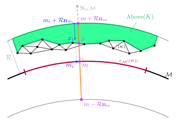
Figure 11: Schematics of the construction in Stage one.

Stage one. We establish the following implication:

$$x\in\operatorname{closure}(\operatorname{Above}(K))\implies[x,m+r\mathbf{n}({m})]\subseteq\operatorname{closure}(\operatorname{Above}(K)).$$

Consider a point $x\in\operatorname{closure}(\operatorname{Above}(K))$, implying the existence of a sequence of points $(x_{i})_{i\in\mathbb{N}}$ in $\operatorname{Above}(K)$ that converges to $x$ as $i\to+\infty$. Let $m=\pi_{\mathcal{M}}(x)$ and $m_{i}=\pi_{\mathcal{M}}(x_{i})$, and consider the sequence of segments $([x_{i},m_{i}+r\mathbf{n}({m_{i}})])_{i\in\mathbb{N}}$ (see Figure 11 for a depiction). Each segment $[x_{i},m_{i}+r\mathbf{n}({m_{i}})]$ in the sequence belongs to $\operatorname{Above}(K)$ since, given $x_{i}\in\operatorname{Above}(K)$, it holds that

$$[x_{i},m_{i}+r\mathbf{n}({m_{i}})]\subseteq[\operatorname{up}_{K}(m_{i}),m_{i}+r\mathbf{n}({m_{i}})]\subseteq\operatorname{Above}(K).$$

Furthermore, we show that the sequence of segments $([x_{i},m_{i}+r\mathbf{n}({m_{i}})])_{i\in\mathbb{N}}$ converges in Hausdorff distance to $[x,m+r\mathbf{n}({m})]$, completing the proof. It is enough to show the convergence of the endpoints of segments and since $\lim_{i\to+\infty}x_{i}=x$, we only need to show that $\lim_{i\to+\infty}(m_{i}+r\mathbf{n}({m_{i}}))=m+r\mathbf{n}({m})$. Let $f:\operatorname{Above}(K)\to\operatorname{Above}(K)$ be defined by $f(z)=\pi_{\mathcal{M}}(z)+r\mathbf{n}({\pi_{\mathcal{M}}(z)})$. Both $\pi_{\mathcal{M}}:\operatorname{Above}(K)\to\mathcal{M}$ and $\mathbf{n}:\mathcal{M}\to\mathbf{n}({m})$ are continuous maps, hence $f$ is continuous and $\lim_{i\to+\infty}f(x_{i})=f(x)$. Thus, $\lim_{i\to+\infty}(m_{i}+r\mathbf{n}({m_{i}}))=m+r\mathbf{n}({m})$.

Stage two. We show that for all $m\in\pi_{\mathcal{M}}(\boldsymbol{\lvert}K\boldsymbol{\rvert})$, the set $A\cap\mathbf{N}_{m}\mathcal{M}\cap B(m,r)$ is connected. Consider two points $x,y\in A\cap\mathbf{N}_{m}\mathcal{M}\cap B(m,r)$. Since $x,y\in\boldsymbol{\lvert}K\boldsymbol{\rvert}\cap\mathbf{N}_{m}\mathcal{M}\cap B(m,r)$, the vertical convexity assumption guarantees that $[x,y]\in\boldsymbol{\lvert}K\boldsymbol{\rvert}\cap\mathbf{N}_{m}\mathcal{M}\cap B(m,r)$. Since $x,y\in\operatorname{closure}(\operatorname{Above}(K))\cap\mathbf{N}_{m}\mathcal{M}\cap B(m,r)$, the previous stage guarantees that $[x,y]\in\operatorname{closure}(\operatorname{Above}(K))\cap\mathbf{N}_{m}\mathcal{M}\cap B(m,r)$. Therefore, $[x,y]$ belongs to $A\cap\mathbf{N}_{m}\mathcal{M}\cap B(m,r)$.

Stage three. We show that $A\cap\mathbf{N}_{m}\mathcal{M}\cap B(m,r)$ is reduced to a single point for all $m\in\pi_{\mathcal{M}}(\boldsymbol{\lvert}K\boldsymbol{\rvert})$. In the previous stage, we established that $A\cap\mathbf{N}_{m}\mathcal{M}\cap B(m,r)$ is connected, thus forming a segment. Assume, for a contradiction, that the endpoints $x$ and $y$ of this segment are distinct. For each $z\in[x,y]$, let $\sigma_{z}$ denote the unique simplex of $K$ containing $z$ in its relative interior. Since $A\subseteq\partial\boldsymbol{\lvert}K\boldsymbol{\rvert}=\boldsymbol{\lvert}\partial K\boldsymbol{\rvert}$, $\sigma_{z}$ belongs to the boundary complex $\partial K$ of $K$ and has $\dim\sigma_{z}<d$ for all $z\in[x,y]$. Given that $x\neq y$, there exists $z\in[x,y]$ with $\dim\sigma_{z}>0$. Since $\sigma_{z}$ is a boundary simplex of $K$ containing $[x,y]$ locally around $z$, it must be vertical with $0<\dim\sigma_{z}<d$, contradicting our assumption that $K$ contains no vertical $i$-simplices for $0<i<d$.

From stage three, $A$ intersects $[m-r\mathbf{n}({m}),m+r\mathbf{n}({m})]$ at a single point for all $m\in\pi_{\mathcal{M}}(\boldsymbol{\lvert}K\boldsymbol{\rvert})$. By construction, so does $\operatorname{UpperSkin}_{\mathcal{M}}(K)$. Since $\operatorname{UpperSkin}_{\mathcal{M}}(K)\subseteq A$, it follows that $\operatorname{UpperSkin}_{\mathcal{M}}(K)=A$ along the normal segment $[m-r\mathbf{n}({m}),m+r\mathbf{n}({m})]$ for all $m\in\pi_{\mathcal{M}}(\boldsymbol{\lvert}K\boldsymbol{\rvert})$. Hence, the upper skin of $K$ coincides with $A$ and is therefore closed.

We are now ready to conclude. The upper skin of $K$ is a closed set and, therefore, compact. The map $\pi_{\mathcal{M}}:\operatorname{UpperSkin}_{\mathcal{M}}(K)\to\pi_{\mathcal{M}}(\boldsymbol{\lvert}K\boldsymbol{\rvert})$ is a continuous bijection from one compact set to another, and is thus a homeomorphism. Let us prove Equation (2), that is,

$$\partial\boldsymbol{\lvert}K\boldsymbol{\rvert}=\operatorname{UpperSkin}_{\mathcal{M}}(K)\cup\operatorname{LowerSkin}_{\mathcal{M}}(K).$$

By definition, the boundary of $\boldsymbol{\lvert}K\boldsymbol{\rvert}$ is the set $\partial\boldsymbol{\lvert}K\boldsymbol{\rvert}=\boldsymbol{\lvert}K\boldsymbol{\rvert}\cap\operatorname{closure}(\mathbb{R}^{d}\setminus\boldsymbol{\lvert}K\boldsymbol{\rvert})$.

Introducing the following sets (see Figure 12)

$$\operatorname{Below}(K) =\bigcup_{m\in\pi_{\mathcal{M}}(\boldsymbol{\lvert}K\boldsymbol{\rvert})}[m-r\mathbf{n}({m}),\operatorname{low}_{K}(m)]\,\,\,\,\text{and}$$

$$\operatorname{Side}(K) =\big{\{}x\in\mathcal{M}^{\oplus r}\mid\pi_{\mathcal{M}}(x)\notin\pi_{\mathcal{M}}(\boldsymbol{\lvert}K\boldsymbol{\rvert})\big{\}},$$

we can write

$$\mathbb{R}^{d}\setminus\boldsymbol{\lvert}K\boldsymbol{\rvert}=\operatorname{Above}(K)\cup\operatorname{Below}(K)\cup(\mathbb{R}^{d}\setminus\mathcal{M}^{\oplus r})\cup\operatorname{Side}(K).$$

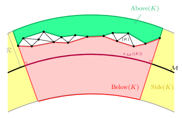
Figure 12: The different regions in $\mathcal{M}^{\oplus r}$.

Taking the closure on both sides, it follows that

$$\operatorname{closure}(\mathbb{R}^{d}\setminus\boldsymbol{\lvert}K\boldsymbol{\rvert}) =\operatorname{closure}(\operatorname{Above}(K))\cup\operatorname{closure}(\operatorname{Below}(K))\cup\operatorname{closure}(\mathbb{R}^{d}\setminus\mathcal{M}^{\oplus r})\cup\operatorname{closure}(\operatorname{Side}(K)).$$

Intersecting both sides of the equality with $\boldsymbol{\lvert}K\boldsymbol{\rvert}$ and noting that the third term in the union has an empty intersection with $\boldsymbol{\lvert}K\boldsymbol{\rvert}$, we obtain that

$$\partial\boldsymbol{\lvert}K\boldsymbol{\rvert} =\boldsymbol{\lvert}K\boldsymbol{\rvert}\cap\operatorname{closure}(\mathbb{R}^{d}\setminus\boldsymbol{\lvert}K\boldsymbol{\rvert})$$

$$=\boldsymbol{\lvert}K\boldsymbol{\rvert}\cap\left(\operatorname{closure}(\operatorname{Above}(K))\cup\operatorname{closure}(\operatorname{Below}(K))\cup\operatorname{closure}(\operatorname{Side}(K))\right)$$

$$=\left(\boldsymbol{\lvert}K\boldsymbol{\rvert}\cap\operatorname{closure}(\operatorname{Above}(K))\right)\cup\left(\boldsymbol{\lvert}K\boldsymbol{\rvert}\cap\operatorname{closure}(\operatorname{Below}(K))\right)$$

$$=\operatorname{UpperSkin}_{\mathcal{M}}(K)\cup\operatorname{LowerSkin}_{\mathcal{M}}(K),$$

which concludes the proof.

See 3.6

Proof B2.

Since $\operatorname{UpperSkin}_{\mathcal{M}}(\boldsymbol{\lvert}K\boldsymbol{\rvert})=\operatorname{LowerSkin}_{\mathcal{M}}(\boldsymbol{\lvert}K\boldsymbol{\rvert})$, it follows that $\operatorname{low}_{\boldsymbol{\lvert}K\boldsymbol{\rvert}}(m)=\operatorname{up}_{\boldsymbol{\lvert}K\boldsymbol{\rvert}}(m)$ for all $m\in\pi_{\mathcal{M}}(\boldsymbol{\lvert}K\boldsymbol{\rvert})$ and $\boldsymbol{\lvert}K\boldsymbol{\rvert}\subseteq\operatorname{UpperSkin}_{\mathcal{M}}(\boldsymbol{\lvert}K\boldsymbol{\rvert})=\operatorname{LowerSkin}_{\mathcal{M}}(\boldsymbol{\lvert}K\boldsymbol{\rvert})$. By Lemma 3.5,

$$\boldsymbol{\lvert}K\boldsymbol{\rvert}\subseteq\operatorname{UpperSkin}_{\mathcal{M}}(\boldsymbol{\lvert}K\boldsymbol{\rvert})\cup\operatorname{LowerSkin}_{\mathcal{M}}(\boldsymbol{\lvert}K\boldsymbol{\rvert})=\partial\boldsymbol{\lvert}K\boldsymbol{\rvert}=\boldsymbol{\lvert}\partial K\boldsymbol{\rvert}.$$

Thus, $\boldsymbol{\lvert}K\boldsymbol{\rvert}\subseteq\boldsymbol{\lvert}\partial K\boldsymbol{\rvert}$ and therefore $K=\partial K$.

By Lemma 3.5, we already know that the union of the upper and lower skins is a simplicial complex. However, since their intersection is non-empty, it is unclear whether each one of them separately is a simplicial complex as well. Lemma 3.7 establishes exactly that, replacing each set in Equation (2) by a simplicial counterpart. Its proof relies on the next lemma.

Lemma B3.

Suppose that $K$ has a non-vertical skeleton and is vertically convex relative to $\mathcal{M}$. Then, for all simplices $\nu\in K$, the following two implications hold:

1. $\operatorname{relint}(\operatorname{conv}(\nu))\cap\operatorname{UpperSkin}_{\mathcal{M}}(K)\neq\emptyset$ $\implies$ $\operatorname{conv}(\nu)\subseteq\operatorname{UpperSkin}_{\mathcal{M}}(K)$;

2. $\operatorname{relint}(\operatorname{conv}(\nu))\cap\operatorname{LowerSkin}_{\mathcal{M}}(K)\neq\emptyset$ $\implies$ $\operatorname{conv}(\nu)\subseteq\operatorname{LowerSkin}_{\mathcal{M}}(K)$.

Proof B4.

Let $\nu$ be a simplex of $K$ and $x\in\operatorname{relint}(\operatorname{conv}(\nu))$. Consider $t>0$ such that the only simplices of $K$ whose convex hull intersects $B(x,t)$ are in the star of $\nu$. We define the geometric star of $x$ in $K$, also known as the tangent cone [35], as

$$\widetilde{\operatorname{St}}_{K}(x)=\Big{\{}\lambda u\mid x+u\in|K|\cap B(x,t),\,\lambda\geq 0\Big{\}}.$$

Similarly, for any $\tau\in\operatorname{St}(\nu,K)$, we introduce the cone

$$\widetilde{\operatorname{St}}_{\tau}(x)=\Big{\{}\lambda u\mid x+u\in\operatorname{relint}(\operatorname{conv}(\tau))\cap B(x,t),\,\lambda\geq 0\Big{\}}.$$

Since $K$ is embedded, the family $\{\widetilde{\operatorname{St}}_{\tau}(x)\mid\tau\in\operatorname{St}(\nu,K)\}$ is a partition of $\widetilde{\operatorname{St}}_{K}(x)$. Note that $x\mapsto\widetilde{\operatorname{St}}_{K}(x)$ remains constant on $\operatorname{relint}(\operatorname{conv}(\nu))$ for each $\nu\in K$, thus depending only on the simplex of $K$ whose support contains $x$ in its relative interior. Additionally, we have:

$$x\in\operatorname{UpperSkin}_{\mathcal{M}}(K)\quad\iff\quad\mathbf{n}({\pi_{\mathcal{M}}(x)})\notin\widetilde{\operatorname{St}}_{K}(x).$$

We next establish that:

$$\operatorname{relint}(\operatorname{conv}(\nu))\cap\operatorname{UpperSkin}_{\mathcal{M}}(K)\neq\emptyset\implies\operatorname{relint}(\operatorname{conv}(\nu))\subseteq\operatorname{UpperSkin}_{\mathcal{M}}(K).$$

If $\dim\nu=0$, the result is clear. For $\dim\nu>0$, assume for contradiction that $x_{0},x_{1}\in\operatorname{relint}(\operatorname{conv}(\nu))$ with $x_{0}\in\operatorname{UpperSkin}_{\mathcal{M}}(K)$ but $x_{1}\notin\operatorname{UpperSkin}_{\mathcal{M}}(K)$. The segment $[x_{0},x_{1}]$ lies entirely within $\operatorname{relint}(\operatorname{conv}(\nu))$. Since $K$ is vertically convex relative to $\mathcal{M}$, there exists $0<r<\operatorname{Reach}(\mathcal{M})$ such that $\boldsymbol{\lvert}K\boldsymbol{\rvert}\subseteq\mathcal{M}^{\oplus r}$. Therefore, the projection map $\pi_{\mathcal{M}}$ is well-defined and continuous on $\boldsymbol{\lvert}K\boldsymbol{\rvert}$, as is the map $x\mapsto\mathbf{n}({\pi_{\mathcal{M}}(x)})$. Consequently, at some point $x\in[x_{0},x_{1}]$, we must have $\mathbf{n}({\pi_{\mathcal{M}}(x)})\in\partial\widetilde{\operatorname{St}}_{K}(x_{0})$, or equivalently:

$$\mathbf{n}({\pi_{\mathcal{M}}(x)})\in\partial\widetilde{\operatorname{St}}_{K}(x).$$

Observe that $\partial\widetilde{\operatorname{St}}_{K}(x)$ is contained in $\bigcup_{\tau}\widetilde{\operatorname{St}}_{\tau}(x)$, where $\tau\in\operatorname{St}(\nu,K)$ has dimension at most $d-1$. Hence, $\mathbf{n}({\pi_{\mathcal{M}}(x)})$ belongs to $\widetilde{\operatorname{St}}_{\tau}(x)$ for some $\tau\in\operatorname{St}(\nu,K)$ with $0<\dim\tau<d$. This implies $\tau$ is vertical with $0<\dim\tau<d$, contradicting the assumption that $K$ has a non-vertical skeleton. It follows that the relative interior of $\nu$ is contained in the upper skin. Moreover, the upper skin is closed, by Lemma 3.5. Hence,

$$\operatorname{relint}(\operatorname{conv}(\nu))\subseteq\operatorname{UpperSkin}_{\mathcal{M}}(K)\implies\operatorname{conv}(\nu)\subseteq\operatorname{UpperSkin}_{\mathcal{M}}(K).$$

The first result, for the upper skin, follows. The proof for the lower skin is analogous.

See 3.7

Proof B5.

By construction, $\boldsymbol{\lvert}\operatorname{UpperComplex}_{\mathcal{M}}(K)\boldsymbol{\rvert}\subseteq\operatorname{UpperSkin}_{\mathcal{M}}(\boldsymbol{\lvert}K\boldsymbol{\rvert})$. For the reverse inclusion, consider $x\in\operatorname{UpperSkin}_{\mathcal{M}}(\boldsymbol{\lvert}K\boldsymbol{\rvert})$ and let $\nu\in K$ be the simplex whose support contains $x$ in its relative interior. By Lemma B3, $\operatorname{conv}(\nu)\subseteq\operatorname{UpperSkin}_{\mathcal{M}}(\boldsymbol{\lvert}K\boldsymbol{\rvert})$, showing that $\nu\in\operatorname{UpperComplex}_{\mathcal{M}}(K)$ and $x\in\boldsymbol{\lvert}\operatorname{UpperComplex}_{\mathcal{M}}(K)\boldsymbol{\rvert}$. We have just established the first equality. The second one is obtained similarly. For the third one, applying Lemma 3.5, we obtain that

$$\boldsymbol{\lvert}\partial K\boldsymbol{\rvert} =\operatorname{UpperSkin}_{\mathcal{M}}(\boldsymbol{\lvert}K\boldsymbol{\rvert})\cup\operatorname{LowerSkin}_{\mathcal{M}}(\boldsymbol{\lvert}K\boldsymbol{\rvert})$$

$$=\boldsymbol{\lvert}\operatorname{UpperComplex}_{\mathcal{M}}(K)\boldsymbol{\rvert}\cup\boldsymbol{\lvert}\operatorname{LowerComplex}_{\mathcal{M}}(K)\boldsymbol{\rvert}$$

$$=\boldsymbol{\lvert}\operatorname{UpperComplex}_{\mathcal{M}}(K)\cup\operatorname{LowerComplex}_{\mathcal{M}}(K)\boldsymbol{\rvert}.$$

Since $\operatorname{UpperComplex}_{\mathcal{M}}(K)\cup\operatorname{LowerComplex}_{\mathcal{M}}(K)\subseteq\partial K$, the third equality follows. Finally, by Lemma 3.5, when $\pi_{\mathcal{M}}(\boldsymbol{\lvert}K\boldsymbol{\rvert})=\mathcal{M}$, both the upper complex and lower complex of $K$ are triangulations of $\mathcal{M}$.

B.2 Upper and lower facets of a $d$-simplex

See 3.8

Proof B6.

By Lemma 3.7 applied with $K=\operatorname{Cl}\sigma$,

$$(\operatorname{Cl}\sigma)^{[d-1]}=\operatorname{UpperFacets}_{\mathcal{M}}(\sigma)\cup\operatorname{LowerFacets}_{\mathcal{M}}(\sigma).$$

Let us show that $\operatorname{UpperFacets}_{\mathcal{M}}(\sigma)\cap\operatorname{LowerFacets}_{\mathcal{M}}(\sigma)=\emptyset$. Suppose for a contradiction that there is a facet $\nu$ of $\sigma$ such that $\operatorname{conv}(\nu)\subseteq\operatorname{UpperSkin}_{\mathcal{M}}(K)$ and $\operatorname{conv}(\nu)\subseteq\operatorname{LowerSkin}_{\mathcal{M}}(K)$. This would imply that $\operatorname{conv}(\sigma)\subseteq\operatorname{Aff}(\nu)$ and $\sigma$ would be degenerate which is impossible. Let us show that $\operatorname{UpperFacets}_{\mathcal{M}}(\sigma)\neq\emptyset$ by contradiction. If $\operatorname{UpperFacets}_{\mathcal{M}}(\sigma)=\emptyset$, then $\operatorname{LowerFacets}_{\mathcal{M}}(\sigma)$ would contain all the facets of $\sigma$, contradicting the fact that the two skins of $\operatorname{Cl}\sigma$ relative to $\mathcal{M}$ are homeomorphic by Lemma 3.5. Similarly, $\operatorname{LowerFacets}_{\mathcal{M}}(\sigma)\neq\emptyset$.

Appendix C Missing proofs of Section 4

C.1 Correctness

See 4.5

Proof C1.

Since the second item of the lemma can be obtained from the first one by reversing the orientation of $\mathcal{M}$, we only need to prove the first item. We start with the forward direction $\Longrightarrow$. Suppose that $\tau\in K$ is a free simplex of $K$ from above relative to $\mathcal{M}$. This implies that

$${\operatorname{St}(\tau,K)}^{[d-1]}=\operatorname{UpperFacets}_{\mathcal{M}}(\sigma),$$

where $\Sigma^{[i]}$ stands for the set of $i$-simplices of $\Sigma$. Observe that $\operatorname{St}(\tau,K)\setminus\{\sigma\}\subseteq\partial K$ and therefore $\operatorname{UpperFacets}_{\mathcal{M}}(\sigma)\subseteq\partial K$. Hence, $\sigma$ has no $d$-simplex in $K$ above it. In other words, $\sigma$ is a sink of the dual graph $G_{\mathcal{M}}(K)$.

Let us prove the backward direction $\Longleftarrow$. Suppose that $\sigma$ is a sink of $G_{\mathcal{M}}(K)$. Equivalently, $\sigma$ is a $d$-simplex of $K$ such that ${\operatorname{UpperFacets}_{\mathcal{M}}(\sigma)}\subseteq\partial K$. By Lemma 3.8, $\operatorname{UpperFacets}_{\mathcal{M}}(\sigma)\neq\emptyset$ and it follows that $\tau\neq\emptyset$ and $\tau\in\partial K$. Let us prove that $\tau$ is a free simplex of $K$. By definition, this boils down to proving that $\operatorname{Lk}(\tau,K)$ is the closure of a simplex. We do this by showing that

$$\operatorname{Lk}(\tau,K)=\operatorname{Lk}(\tau,\operatorname{Cl}\sigma).$$ (14)

We first claim that the above equation is implied by the following one

$$\operatorname{Lk}(\tau,\partial K)=\operatorname{Lk}(\tau,\partial\operatorname{Cl}\sigma).$$ (15)

Indeed, suppose that we have (15). Since $\operatorname{Cl}\sigma\subseteq K$, we get that $\operatorname{Lk}(\tau,\operatorname{Cl}\sigma)\subseteq\operatorname{Lk}(\tau,K)$ and we only need to establish the reverse inclusion to get (14). For this, we use the fact that for any simplicial complex $X$ embedded in $\mathbb{R}^{d}$ and any $\tau\in X$, we have that $\partial\operatorname{Lk}(\tau,X)=\operatorname{Lk}(\tau,\partial X)$. We thus deduce from (15) that

$$\partial\operatorname{Lk}(\tau,K)=\partial\operatorname{Lk}(\tau,\operatorname{Cl}\sigma).$$

Because $\tau\in\partial K$, it follows that $\boldsymbol{\lvert}\operatorname{Lk}(\tau,K)\boldsymbol{\rvert}$ is topologically equivalent to a proper subset of the $(d-k-1)$-sphere, where $k=\dim\tau$. Because $\tau\in\partial\operatorname{Cl}\sigma$, we have similarly that $\boldsymbol{\lvert}\operatorname{Lk}(\tau,\operatorname{Cl}\sigma)\boldsymbol{\rvert}$ is also topologically equivalent to a proper subset of the $(d-k-1)$-sphere. Since the latter link is a subset of the former link and the two links share the same boundary complex, the only possibility is that they are equal and we get (14). We have just established our claim that (15) $\implies$ (14). Hence, to prove that $\tau$ is a free simplex of $K$, it suffices to establish (15). Let

A $$=\operatorname{Lk}(\tau,\partial K)$$

B $$=\operatorname{Lk}(\tau,\operatorname{UpperComplex}_{\mathcal{M}}(K))$$

C $$=\operatorname{Lk}(\tau,\operatorname{UpperComplex}_{\mathcal{M}}(\operatorname{Cl}\sigma))$$

D $$=\operatorname{Lk}(\tau,\partial\operatorname{Cl}\sigma).$$

We prove (15) by showing that $\mbox{\bf A}=\mbox{\bf B}=\mbox{\bf C}=\mbox{\bf D}$ in three steps. Before we start, we write two useful equalities due to the fact $\partial\operatorname{Cl}\sigma$ is a pure simplicial $(d-1)$-complex:

$$\operatorname{Cl}(\operatorname{UpperFacets}_{\mathcal{M}}(\sigma)) =\operatorname{UpperComplex}_{\mathcal{M}}(\operatorname{Cl}\sigma),$$ (16)

$$\operatorname{Cl}(\operatorname{LowerFacets}_{\mathcal{M}}(\sigma)) =\operatorname{LowerComplex}_{\mathcal{M}}(\operatorname{Cl}\sigma).$$ (17)

We refer the reader to Figure 13 for a pictorial representation of the objects in the proof.

Figure 13: Notation for the proof of Lemma 4.5. The upper skin of $K$ is in green and its lower skin in pink. We have schematically represented $\sigma$ using curved edges. Its upper skin (in pale green) is a subset of the upper skin of $K$. The $k$-simplex $\tau$ is represented as a black dot. Its link in $\partial K$ is represented by the two white dots and is proved to triangulate the $(d-k-2)$-sphere.

Step 1: $\mbox{\bf A}=\mbox{\bf B}$. By Lemma 3.8, $\operatorname{UpperFacets}_{\mathcal{M}}(\sigma)$ and $\operatorname{LowerFacets}_{\mathcal{M}}(\sigma)$ partition the facets of $\sigma$. Let us make a general observation. Suppose that $\Sigma$ and $\Sigma^{\prime}$ partition the set of facets of $\sigma$. Let $\tau=\bigcap\Sigma$ and consider a point $x$ in the relative interior of $\operatorname{conv}(\Sigma)$. Since $\operatorname{Cl}\sigma$ is embedded, $x$ does not lie on $\boldsymbol{\lvert}\operatorname{Cl}(\Sigma^{\prime})\boldsymbol{\rvert}$. Applying this with $\Sigma=\operatorname{UpperFacets}_{\mathcal{M}}(\sigma)$ and $\Sigma^{\prime}=\operatorname{LowerFacets}_{\mathcal{M}}(\sigma)$, we get that for any point $x$ in the relative interior of $\operatorname{conv}(\sigma)$, we have that

$$x\not\in\boldsymbol{\lvert}\operatorname{Cl}(\operatorname{LowerFacets}_{\mathcal{M}}(\sigma))\boldsymbol{\rvert}=\boldsymbol{\lvert}\operatorname{LowerComplex}_{\mathcal{M}}(\operatorname{Cl}\sigma)\boldsymbol{\rvert}=\operatorname{LowerSkin}_{\mathcal{M}}(\operatorname{Cl}\sigma),$$

where the first equality comes from (17) and the second equality comes from Lemma 3.7. Let $m=\pi_{\mathcal{M}}(x)$. By construction, the normal segment $\mathbf{N}_{m}\mathcal{M}\cap B(m,r)$ passes through $x$. It intersects $\operatorname{LowerSkin}_{\mathcal{M}}(\operatorname{Cl}\sigma)$ in a point $y$ and $\operatorname{LowerSkin}_{\mathcal{M}}(K)$ in a point $z$ in such a way that along direction $\mathbf{n}({m})$, $x$ is strictly above $y$ and $z$ cannot be above $y$. This shows that $x\neq z$ and consequently $x\not\in\operatorname{LowerSkin}_{\mathcal{M}}(K)$. Since $\operatorname{LowerSkin}_{\mathcal{M}}(K)$ is a closed set by Lemma 3.5, $x$ is at distance greater than some $\epsilon>0$ of $\operatorname{LowerSkin}_{\mathcal{M}}(K)$. It follows that

$$B(x,\epsilon)\cap\boldsymbol{\lvert}\partial K\boldsymbol{\rvert}=B(x,\epsilon)\cap\boldsymbol{\lvert}\operatorname{UpperComplex}_{\mathcal{M}}(K)\boldsymbol{\rvert}.$$

Since $K$ is canonically embedded, the star (and therefore the link) of $\tau$ in any subcomplex of $K$ depends only upon simplices whose support intersects some neighborhood of $x$. It follows that:

$$\operatorname{Lk}(\tau,\partial K)=\operatorname{Lk}(\tau,\operatorname{UpperComplex}_{\mathcal{M}}(K)).$$

Step 2: $\mbox{\bf C}=\mbox{\bf D}$. Consider again two sets $\Sigma$ and $\Sigma^{\prime}$ that partition the set of facets of $\sigma$. Setting $\tau=\bigcap\Sigma$, one can observe that $\operatorname{Lk}(\tau,\operatorname{Cl}(\Sigma))=\operatorname{Lk}(\tau,\partial\operatorname{Cl}\sigma)$. Applying this with $\Sigma=\operatorname{UpperFacets}_{\mathcal{M}}(\sigma)$ and $\Sigma^{\prime}=\operatorname{LowerFacets}_{\mathcal{M}}(\sigma)$ and using (16), we get that

$$\operatorname{Lk}(\tau,\operatorname{UpperComplex}_{\mathcal{M}}(\operatorname{Cl}\sigma))=\operatorname{Lk}(\tau,\partial\operatorname{Cl}\sigma).$$

We see in particular that $\boldsymbol{\lvert}\operatorname{Lk}(\tau,\operatorname{UpperComplex}_{\mathcal{M}}(\operatorname{Cl}\sigma))\boldsymbol{\rvert}$ is a topological $(d-k-2)$-sphere.

Step 3: $\mbox{\bf B}=\mbox{\bf C}$. Recall that ${\operatorname{UpperFacets}_{\mathcal{M}}(\sigma)}\subseteq\partial K$. By Lemma 3.7, $\partial K$ is the union of the two subcomplexes $\operatorname{UpperComplex}_{\mathcal{M}}(K)$ and $\operatorname{LowerComplex}_{\mathcal{M}}(K)$ whose underlying spaces are the upper and lower skins of $K$ relative to $\mathcal{M}$, respectively. Each upper facet of $\sigma$ is contained in one of those two skins but not both. The only possibility is thus that $\operatorname{UpperFacets}_{\mathcal{M}}(\sigma)\subseteq\operatorname{UpperComplex}_{\mathcal{M}}(K)$ and therefore using (16)

$$\operatorname{UpperComplex}_{\mathcal{M}}(\operatorname{Cl}\sigma)\subseteq\operatorname{UpperComplex}_{\mathcal{M}}(K).$$

Taking the link of $\tau$ in each of those two subcomplexes of $K$, we get that

$$\operatorname{Lk}(\tau,\operatorname{UpperComplex}_{\mathcal{M}}(\operatorname{Cl}\sigma))\subseteq\operatorname{Lk}(\tau,\operatorname{UpperComplex}_{\mathcal{M}}(K)).$$

On the left side, we know from the previous step that the link is a triangulation of the $(d-k-2)$-sphere. We now study the link on the right side. By Lemma 3.5, $\boldsymbol{\lvert}\operatorname{UpperComplex}_{\mathcal{M}}(K)\boldsymbol{\rvert}$ is homeomorphic to $\mathcal{M}$. Since $\mathcal{M}$ is a $(d-1)$-manifold without boundary, we deduce that so is $\boldsymbol{\lvert}\operatorname{UpperComplex}_{\mathcal{M}}(K)\boldsymbol{\rvert}$. This implies that the link of any simplex in $\operatorname{UpperComplex}_{\mathcal{M}}(K)$ is a triangulation of the $(d-k-2)$-sphere. In summary, writing $X\approx Y$ if $X$ is homeomorphic to $Y$ and $\mathbb{S}^{i}$ for the $i$-sphere, we obtain that

$$\mathbb{S}^{d-k-2}\,\approx\,\boldsymbol{\lvert}\operatorname{Lk}(\tau,\operatorname{UpperComplex}_{\mathcal{M}}(\operatorname{Cl}\sigma))\boldsymbol{\rvert}\,\subseteq\,\boldsymbol{\lvert}\operatorname{Lk}(\tau,\operatorname{UpperComplex}_{\mathcal{M}}(K))\boldsymbol{\rvert}\,\approx\,\mathbb{S}^{d-k-2}.$$

The only subset of $\mathbb{S}^{d-k-2}$ homeomorphic to $\mathbb{S}^{d-k-2}$ being $\mathbb{S}^{d-k-2}$ itself, we get that:

$$\operatorname{Lk}(\tau,\operatorname{UpperComplex}_{\mathcal{M}}(\operatorname{Cl}\sigma))=\operatorname{Lk}(\tau,\operatorname{UpperComplex}_{\mathcal{M}}(K))$$

We have just proved that $\tau$ is a free simplex of $K$. Clearly, $\tau$ is then also free from above with respect to $\mathcal{M}$ since its coface $\sigma$ has dimension $d$ and its $(d-1)$-cofaces are the upper facets of $\sigma$ by construction. This concludes the proof.

See 4.6

Proof C2.

Because $K^{\prime}\subseteq K$, clearly $\boldsymbol{\lvert}K^{\prime}\boldsymbol{\rvert}\subseteq\mathcal{M}^{\oplus r}$ and $K^{\prime}$ has a non-vertical skeleton with respect to $\mathcal{M}$. Let us establish vertical convexity and covering projection for $K^{\prime}$. Because $\tau$ is a vertically free simplex in $K$ relative to $\mathcal{M}$, the star $\operatorname{St}(\tau,K)$ has a unique inclusion-maximal simplex $\sigma$ whose dimension is $d$. Furthermore, one of the following two situations occurs:

$$\text{(1) }{\operatorname{St}(\tau,K)}^{[d-1]}=\operatorname{UpperFacets}_{\mathcal{M}}(\sigma)\quad\text{or}\quad\text{(2) }{\operatorname{St}(\tau,K)}^{[d-1]}=\operatorname{LowerFacets}_{\mathcal{M}}(\sigma),$$

where $\Sigma^{[i]}$ stands for the set of $i$-simplices of $\Sigma$. Suppose that situation (1) occurs. In other words, $\tau$ is a free simplex of $K$ from above relative to $\mathcal{M}$. This implies that the upper skin of $\boldsymbol{\lvert}\sigma\boldsymbol{\rvert}$ is contained in the upper skin of $\boldsymbol{\lvert}K\boldsymbol{\rvert}$ and $\operatorname{up}_{\operatorname{Cl}\sigma}(m)=\operatorname{up}_{K}(m)$ for all $m\in\pi_{\mathcal{M}}(\operatorname{conv}(\sigma))$. We deduce that:

$$\boldsymbol{\lvert}K^{\prime}\boldsymbol{\rvert}\cap\mathbf{N}_{m}\mathcal{M}\cap B(m,r)=\begin{cases}[\operatorname{low}_{K}(m),\operatorname{low}_{\operatorname{Cl}\sigma}(m)]&\text{if $m\in\pi_{\mathcal{M}}(\operatorname{conv}(\sigma))$},\\ \boldsymbol{\lvert}K\boldsymbol{\rvert}\cap\mathbf{N}_{m}\mathcal{M}\cap B(m,r)&\text{otherwise}.\end{cases}$$

We conclude that $K^{\prime}$ is both vertically convex relative to $\mathcal{M}$ and has a covering projection. Similarly, we obtain the same conclusion when situation (2) occurs. It remains to check that the acyclicity condition holds for $K^{\prime}$ as well. Note that acyclicity of the relation $\prec_{\mathcal{M}}$ over $d$-simplices of $K$ is equivalent to acyclicity of the graph $G_{\mathcal{M}}(K)$. By Lemma 4.5, a vertical collapse in $K$ corresponds to the removal of a terminal node of $G_{\mathcal{M}}(K)$. We thus obtain acyclicity of the graph $G_{\mathcal{M}}(K^{\prime})$ or, equivalently, acyclicity of the relation $\prec_{\mathcal{M}}$ over $d$-simplices of $K^{\prime}$.

C.2 Practical version

See 4.8

Proof C3.

Let $\tau$ be a free simplex of $K$ whose inclusion-maximal coface $\sigma$ has dimension $d$. We prove the theorem by establishing the following equivalence: $\tau$ is vertically free in $K$ relative to $\mathcal{M}$ if and only if $\tau$ is vertically free in $K$ relative to $\mathcal{H}_{\tau}$.

For any facet $\nu$ of $\sigma$, let $N_{\nu}$ denote the unit normal to $\operatorname{conv}(\nu)$ pointing outwards $\operatorname{conv}(\sigma)$, as illustrated in Figure 14. We have assumed that for any facet $\nu$ of $\sigma$ and any vertex $a$ of $\nu$:

$$\angle(\operatorname{Aff}(\nu),\mathbf{T}_{\pi_{\mathcal{M}}(a)}\mathcal{M})\,<\,\frac{\pi}{4}.$$

It follows that for any facet $\nu$ of $\sigma$ and any vertex $a\in\nu$,

$$\angle(\mathbf{n}({\pi_{\mathcal{M}}(a)}),N_{\nu}) <\frac{\pi}{4}, \text{if $\nu\in\operatorname{UpperFacets}_{\mathcal{M}}(\sigma)$},$$

$$\angle(\mathbf{n}({\pi_{\mathcal{M}}(a)}),N_{\nu}) >\frac{3\pi}{4}, \text{if $\nu\in\operatorname{LowerFacets}_{\mathcal{M}}(\sigma)$}.$$

Figure 14: Outward-pointing normal vectors to a triangle in $\mathbb{R}^{2}$ can be partitioned in two groups, depending on the angle they make. One of the group consists of normal vectors to upper facets of $\sigma$, the other group consists of normal vectors to lower facets of $\sigma$.

Given any pair of facets $\nu_{0},\nu_{1}$ of $\sigma$, we note that we can always find a common vertex $a\in\nu_{0}\cap\nu_{1}$. It follows that $\angle(N_{\nu_{0}},N_{\nu_{1}})<\frac{\pi}{2}$ if $\nu_{0}$ and $\nu_{1}$ are both upper facets of $\sigma$ relative to $\mathcal{M}$ or both lower facets of $\sigma$ relative to $\mathcal{M}$ and $\angle(N_{\nu_{0}},N_{\nu_{1}})>\frac{\pi}{2}$ otherwise. We can thus partition the facets of $\sigma$ in two groups, depicted in two different colors in Figure 14. In each group, any two facets have their outward-pointing normal vectors that make an angle smaller than $\frac{\pi}{2}$. Two facets not in the same group have their outward-pointing normal vectors making an angle greater than $\frac{\pi}{2}$. Let $\nu$ be any facet of $\sigma$. Let $N$ be one of the two unit normal vectors to $\operatorname{Aff}(\nu)$ and use it to orient $\operatorname{Aff}(\nu)$. If $N=N_{\nu}$ (resp. $N=-N_{\nu}$), facets in the group of $\nu$ are precisely those that are upper (resp. lower) facets of $\sigma$ relative to $\operatorname{Aff}(\nu)$. We thus deduce that either

$$\begin{cases}\operatorname{UpperFacets}_{\mathcal{M}}(\sigma)=\operatorname{UpperFacets}_{\operatorname{Aff}(\nu)}(\sigma),\\ \operatorname{LowerFacets}_{\mathcal{M}}(\sigma)=\operatorname{LowerFacets}_{\operatorname{Aff}(\nu)}(\sigma),\end{cases}$$

or

$$\begin{cases}\operatorname{UpperFacets}_{\mathcal{M}}(\sigma)=\operatorname{LowerFacets}_{\operatorname{Aff}(\nu)}(\sigma),\\ \operatorname{LowerFacets}_{\mathcal{M}}(\sigma)=\operatorname{UpperFacets}_{\operatorname{Aff}(\nu)}(\sigma),\end{cases}$$

depending upon the choice of $N$ to orient $\operatorname{Aff}(\nu)$. The result follows immediately by noting that for $\mathcal{X}\in\{\mathcal{M},\operatorname{Aff}(\nu)\}$, the simplex $\tau$ is vertically free in $K$ relative to $\mathcal{X}$ if and only if

$${\operatorname{St}(\tau,K)}^{[d-1]}=\operatorname{UpperFacets}_{\mathcal{X}}(\sigma)\quad\text{or}\quad{\operatorname{St}(\tau,K)}^{[d-1]}=\operatorname{LowerFacets}_{\mathcal{X}}(\sigma),$$

where $\Sigma^{[i]}$ stands for the set of $i$-simplices of $\Sigma$. Thus, $\tau$ is vertically free in $K$ relative to $\mathcal{M}$ if and only if $\tau$ is vertically free in $K$ relative to $\operatorname{Aff}(\nu)$. We get the desired equivalence.

Appendix D Additional material for Section 5

This appendix contains missing material for Section 5.

D.1 Definition of $I(\varepsilon,\delta)$

We define $I(\varepsilon,\delta)$ as the range of values of $\alpha$ used in [8] for Theorem 5.2. Following [8], we define $I(\varepsilon,\delta)$ by distinguishing two cases. If $\delta\geq\varepsilon$, then the authors in [8] establish that the following interval of values for $\alpha$ is valid:

$$I(\varepsilon,\delta)=\left[\frac{1}{2}\left(\mathcal{R}+\varepsilon-\sqrt{\Delta_{0}}\right),\frac{1}{2}\left(\mathcal{R}+\varepsilon+\sqrt{\Delta_{0}}\right)\right],$$

where $\Delta_{0}=2(\mathcal{R}-\delta)^{2}-(\mathcal{R}+\varepsilon)^{2}$. The definition of $I(\varepsilon,\delta)$ is more involved when $\delta\leq\varepsilon$. Let

$$\Delta_{1}=\frac{1}{\mathcal{R}^{2}}\left(\varepsilon^{2}-\left(\mathcal{R}-\delta\right)^{2}\right)^{2}-10\left(\varepsilon^{2}-\left(\mathcal{R}-\delta\right)^{2}\right)-7\mathcal{R}^{2}.$$

Assuming that $\varepsilon<\mathcal{R}$ and $\delta<\mathcal{R}$ satisfy the strict homotopy condition:

$$(\mathcal{R}-\delta)^{2}-\varepsilon^{2}\geq(4\sqrt{2}-5)\mathcal{R}^{2},$$

it has been shown in [8] that $\Delta_{1}$ is non-negative and thus, it makes sense to define

$$\beta_{\min}=\frac{1}{4}\left(\frac{(\mathcal{R}-\delta)^{2}+\mathcal{R}^{2}-\varepsilon^{2}}{\mathcal{R}}-\sqrt{\Delta_{1}}\right)\quad\text{ and }\quad\beta_{\max}=\frac{1}{4}\left(\frac{(\mathcal{R}-\delta)^{2}+\mathcal{R}^{2}-\varepsilon^{2}}{\mathcal{R}}+\sqrt{\Delta_{1}}\right).$$

$\Delta_{1}$ in [8] has been chosen precisely to be the discriminant of the quadratic polynomial:

$$\varepsilon^{2}-\left(\mathcal{R}-\delta\right)^{2}+\mathcal{R}^{2}+\beta\,\frac{1}{\mathcal{R}}\left(\varepsilon^{2}-\mathcal{R}^{2}-\left(\mathcal{R}-\delta\right)^{2}\right)+2\beta^{2}$$

and $[\beta_{\min},\beta_{\max}]$ represents the interval of values of $\beta$ for which the polynomial is non-negative. The non-negativity can be rewritten as:

$$\left(1+\frac{\beta}{\mathcal{R}}\right)\varepsilon^{2}+\beta^{2}+\frac{\beta}{\mathcal{R}}\left(\mathcal{R}^{2}-(\mathcal{R}-\delta)^{2}\right)\,\leq\,(\mathcal{R}-\delta)^{2}-(\mathcal{R}-\beta)^{2}.$$ (18)

Let

$$\alpha_{\min} =\sqrt{\left(1+\frac{\beta_{\min}}{\mathcal{R}}\right)\varepsilon^{2}+\beta_{\min}^{2}+\frac{\beta_{\min}}{\mathcal{R}}\left(\mathcal{R}^{2}-(\mathcal{R}-\delta)^{2}\right)},$$

$$\alpha_{\max} =\sqrt{(\mathcal{R}-\delta)^{2}-(\mathcal{R}-\beta_{\max})^{2}},$$

Equation (18) shows that $\alpha_{\min}\leq\alpha_{\max}$. It is then proven in [8] that when $\delta\leq\varepsilon$ the non-empty interval $I(\varepsilon,\delta)=[\alpha_{\min},\alpha_{\max}]$ can be used for Theorem 5.2.

D.2 Possible $\beta$ for Theorem 5.3

The next lemma enunciates a result of [8] that provides a “large” value of $\beta$ for which $\mathcal{M}^{\oplus\beta}\subseteq P^{\oplus\alpha}$ and which can be plugged in Theorem 5.3.

Lemma D1 ([8]).

Let $\mathcal{M}$ be a smooth submanifold whose reach is larger than or equal to $\mathcal{R}$ and let $P$ be a point set such that $\mathcal{M}\subseteq P^{\oplus\varepsilon}$ for some $\varepsilon\geq 0$. Then, $\mathcal{M}^{\oplus\beta}\subseteq P^{\oplus\alpha}$ whenever

$$\beta=-\frac{\varepsilon^{2}}{2\mathcal{R}}+\sqrt{\alpha^{2}+\frac{\varepsilon^{4}}{4\mathcal{R}^{2}}-\varepsilon^{2}}.$$

Appendix E Proof of Theorem 5.3 in Section 5

The goal of this appendix is to establish Theorem 5.3:

See 5.3

Remark E1.

It is easy to check that Conditions (5), (6) and (7) in Theorem 5.3 are well-defined. Because $P\subseteq\mathcal{M}^{\oplus\delta}$, we obtain that $\boldsymbol{\lvert}\operatorname{Del}(P,\alpha)\boldsymbol{\rvert}\subseteq P^{\oplus\alpha}\subseteq\mathcal{M}^{\oplus(\delta+\alpha)}$. Since $\delta+\alpha<\mathcal{R}\leq\operatorname{Reach}(\mathcal{M})$,

$$\boldsymbol{\lvert}\operatorname{Del}(P,\alpha)\boldsymbol{\rvert}\subseteq\mathbb{R}^{d}\setminus\operatorname{axis}(\mathcal{M})$$

and the projection map $\pi_{\mathcal{M}}$ is thus well-defined on the support of any simplex in $\operatorname{Del}(P,\alpha)$. It follows that the left sides of Conditions (5), (6) and (7) are well-defined. We claim that

$$-1\leq\frac{(\mathcal{R}+\beta)^{2}-(\mathcal{R}+\delta)^{2}-\alpha^{2}}{2(\mathcal{R}+\delta)\alpha}\leq 1.$$

The left inequality is equivalent to $\beta+\alpha\geq\delta$ which holds since we have assumed that $\alpha\geq\delta$. The right inequality is equivalent to $\beta\leq\delta+\alpha$ which holds because we have assumed that $P\subseteq\mathcal{M}^{\oplus\delta}$ and $\mathcal{M}^{\oplus\beta}\subseteq P^{\oplus\alpha}$, implying that $\mathcal{M}^{\oplus\beta}\subseteq\mathcal{M}^{\oplus(\delta+\alpha)}$. Hence, the right side of Condition (6) is well-defined. Similarly, using the assumption $\alpha\leq\frac{2}{3}(\mathcal{R}-\delta)$, we easily get that

$$0\leq\frac{\alpha}{2(\mathcal{R}-\delta-\alpha)}\leq 1,$$

showing that the right side of Condition (7) is also well-defined.

Proof E2 (Proof of Theorem 5.3.).

Injective projection for $\operatorname{Del}(P,\alpha)$ is shown in Section E.1 (Lemma E3). Covering projection and vertical convexity for $\operatorname{Del}(P,\alpha)$ are established in Section 5.2 (Lemma 5.5). Acyclicity is established in Section E.3 (Lemma E11). Hence, all the assumptions of Lemma 3.7 and Theorem 4.4 are satisfied. By Lemma 3.7, the upper and lower complexes of $\operatorname{Del}(P,\alpha)$ relative to $\mathcal{M}$ are each a triangulation of $\mathcal{M}$. By Theorem 4.4, $\operatorname{\tt NaiveSquash}(P,\alpha)$ returns a triangulation of $\mathcal{M}$.

E.1 Injective projection

In this section, we characterize non-verticality of an $i$-simplex $\tau\in\operatorname{Del}(P,\alpha)$ relative to $\mathcal{M}$.

Lemma E3.

Let $P$ be a finite point set in $\mathbb{R}^{d}$ such that $P\subseteq\mathcal{M}^{\oplus\delta}$ for some $\delta\geq 0$. Let $\alpha\in[0,\mathcal{R}-\delta)$. Then, for all $i$-simplices $\tau\in\operatorname{Del}(P,\alpha)$ with $0<i<d$,

$$\eqref{eq:angle-condition-for-skeleton}\quad\iff\quad\text{$\tau$ is non-vertical relative to $\mathcal{M}$}$$

Proof E4.

It is easy to see that $\tau$ is non-vertical relative to $\mathcal{M}$ if and only if for all $x\in\operatorname{conv}(\tau)$

$$\angle(\mathbf{N}_{\pi_{\mathcal{M}}(x)}\mathcal{M},\operatorname{Aff}(\tau)))>0.$$

Using Property A2, $\angle(\mathbf{N}_{\pi_{\mathcal{M}}(x)}\mathcal{M},\operatorname{Aff}(\tau)))=\frac{\pi}{2}-\angle(\operatorname{Aff}(\tau),\mathbf{T}_{\pi_{\mathcal{M}}(x)}\mathcal{M})$ and the above inequality is equivalent to $\angle(\operatorname{Aff}(\tau),\mathbf{T}_{\pi_{\mathcal{M}}(x)}\mathcal{M})<\frac{\pi}{2}.$ Hence, $\tau$ is non-vertical relative to $\mathcal{M}$ if and only if

$$\max_{x\in\operatorname{conv}(\tau)}\angle(\operatorname{Aff}(\tau),\mathbf{T}_{\pi_{\mathcal{M}}(x)}\mathcal{M})\,<\,\frac{\pi}{2},$$

which is equivalent to (5).

E.2 Vertical convexity

In this section, we establish Lemma 5.8, which we need for the proof of Lemma 5.5.

See 5.8

Plugging the assumptions of Lemma 5.5 inside Lemma 5.8 and using Lemma E3 to replace Condition (5) with the assumption that $\tau$ is non-vertical relative to $\mathcal{M}$, we can rewrite Lemma 5.8 as follows:

Lemma E5.

Let $\mathcal{M}\subseteq P^{\oplus\varepsilon}$ and $P\subseteq\mathcal{M}^{\oplus\delta}$ for some $\varepsilon,\delta\geq 0$ that satisfy the strict homotopy condition. Let $\alpha\in[\delta,\mathcal{R}-\delta)\cap I{(\varepsilon,\delta)}$ and $\beta>0$ be such that $\mathcal{M}^{\oplus\beta}\subseteq P^{\oplus\alpha}$. Suppose that for all $i$-simplices $\tau\in\operatorname{Del}(P,\alpha)$ with $0<i<d$, $\tau$ is non-vertical relative to $\mathcal{M}$ and Condition (6) hold. Let $\gamma\in\operatorname{Del}(P,\alpha)$ and $x\in\operatorname{relint}(\operatorname{conv}(\gamma))$. If for some $\lambda>0$ (resp. $\lambda<0$), the segment $(x,x+\lambda\mathbf{n}({\pi_{\mathcal{M}}(x)})]$ lies outside $\boldsymbol{\lvert}\operatorname{Del}(P,\alpha)\boldsymbol{\rvert}$, then it intersects an upper (resp. lower join).

Figure 15: For $d=2$ and $\gamma=\{a,b\}$, the set $S(\gamma,\alpha)$ is a 0-sphere that consists of the two white dots. Only one of them lies on $\partial P^{\oplus\alpha}$ and therefore belongs to $F_{\gamma}$. In this particular case, $F_{\gamma}^{+}=F_{\gamma}$.

Hence, proving Lemma 5.8 is equivalent to proving Lemma E5. Before giving the proof at the end of the section, consider a finite point set $P\subseteq\mathbb{R}^{d}$ and recall that, as explained in Section 5.2, the boundary of $P^{\oplus\alpha}$ can be decomposed into faces. Those faces are in one-to-one correspondence with the boundary simplices of $\operatorname{Del}(P,\alpha)$. Associate to each boundary $i$-simplex $\gamma\in\partial\operatorname{Del}(P,\alpha)$ the $(d-i-1)$-sphere

$$S(\gamma,\alpha)=\bigcap_{p\in\gamma}\partial B(p,\alpha).$$

Equivalently, $S(\gamma,\alpha)$ can be defined as the locus of the centers of the $(d-1)$-spheres with radius $\alpha$ that circumscribe $\gamma$. The center $c_{\gamma}$ of $S(\gamma,\alpha)$ coincides with the center of the smallest $(d-1)$-sphere circumscribing $\gamma$; see Figure 15. The face of $\partial P^{\oplus\alpha}$ dual to $\gamma\in\partial\operatorname{Del}(P,\alpha)$ can then be described as

$$F_{\gamma}=S(\gamma,\alpha)\cap\partial P^{\oplus\alpha}.$$

We also recall that the upper face $F_{\gamma}^{+}$ (resp. lower face $F_{\gamma}^{-}$) designates the restriction of $F_{\gamma}$ to the upper skin (resp. lower skin) of $P^{\oplus\alpha}$. The set $F_{\gamma}^{+}*\operatorname{conv}(\gamma)$ (resp. $F_{\gamma}^{-}*\operatorname{conv}(\gamma)$) designates the upper (resp. lower) join of $\gamma$.

Figure 16: Highest point $s_{\gamma}(x)$ of $S(\gamma,\alpha)$ in direction $\mathbf{n}({x^{*}})$ when $\mathcal{M}$ is a surface in $\mathbb{R}^{3}$ and $\dim\gamma=0$ (left), $\dim\gamma=1$ (middle), and $\dim\gamma=2$ (right).

More generally, given any simplex $\gamma\subseteq\mathbb{R}^{d}$ (not necessarily in $\operatorname{Del}(P,\alpha)$), we define $S(\gamma,\alpha)=\bigcap_{p\in\gamma}\partial B(p,\alpha)$. Assuming that $\operatorname{conv}(\gamma)\subseteq\mathbb{R}^{d}\setminus\operatorname{axis}(\mathcal{M})$ and $S(\gamma,\alpha)\neq\emptyset$, we associate to $\gamma$ and any $x\in\operatorname{conv}(\gamma)$ the highest point of $S(\gamma,\alpha)$ in direction $\mathbf{n}({\pi_{\mathcal{M}}(x)})$ which we denote as $s_{\gamma}(x)$; see Figure 16. Let $\operatorname{Bis}(\gamma)$ be the bisector of $\gamma$. By construction, $s_{\gamma}(x)\in S(\gamma,\alpha)\subseteq\operatorname{Bis}(\gamma)$. Writing $x^{*}=\pi_{\mathcal{M}}(x)$ for short, we make the following remark:

Remark E6.

For any simplex $\gamma\subseteq\mathbb{R}^{d}$ and $\alpha\geq 0$ such that $\operatorname{conv}(\gamma)\subseteq\mathbb{R}^{d}\setminus\operatorname{axis}(\mathcal{M})$ and $S(\gamma,\alpha)\neq\emptyset$ and for any $x\in\operatorname{conv}(\gamma)$,

$$\angle(\mathbf{n}({x^{*}}),s_{\gamma}(x)-c_{\gamma})=\angle(\mathbf{N}_{x^{*}}\mathcal{M},\operatorname{Bis}(\gamma))=\angle(\operatorname{Aff}(\gamma),\mathbf{T}_{x^{*}}\mathcal{M}).$$

We start with a lemma.

Lemma E7.

Assume that $\mathcal{M}\subseteq P^{\oplus\varepsilon}$ and $P\subseteq\mathcal{M}^{\oplus\delta}$ for some $\varepsilon,\delta\geq 0$ and let $\alpha\in[\delta,\mathcal{R}-\delta)$. Let $\beta>0$ such that $\mathcal{M}^{\oplus\beta}\subseteq P^{\oplus\alpha}$. Consider a simplex $\tau$ with $0<\dim\tau<d$ that satisfies (6). Suppose that $\tau$ is a boundary simplex of $\operatorname{Del}(P,\alpha)$. Then, we can always find $a\in\tau$ at which the following implication holds:

$$s_{\tau}(a)\text{ lies on }\partial P^{\oplus\alpha}\quad\implies\quad s_{\tau}(a)\text{ lies on the upper skin of }P^{\oplus\alpha}.$$ (19)

Figure 17: We reach a contradiction in the proof of Lemma E7 by assuming that $s_{\tau}(a)$ lies on the lower skin of $\partial P^{\oplus\alpha}$.

Proof E8.

Because $\tau$ is a boundary simplex of $\operatorname{Del}(P,\alpha)$, we have that $S(\tau,\alpha)\neq\emptyset$ and for any $x\in\operatorname{conv}(\tau)$, the point $s_{\tau}(x)$ exists. Consider $a\in\tau$ and write $a^{*}=\pi_{\mathcal{M}}(a)$ for short. Suppose that $a\in\tau$ is such that

$$s_{\tau}(a)\text{ lies on }\partial P^{\oplus\alpha}\quad\text{ and }\quad s_{\tau}(a)\text{ does not lie on the upper skin of }P^{\oplus\alpha}.$$ (20)

The only possibility is thus that $s_{\tau}(a)$ lies on the lower skin of $P$, as illustrated in Figure 17. Let $z={a^{*}}+\mathcal{R}\mathbf{n}({a^{*}})$ and note that the ball $B(z,\mathcal{R})$ is tangent to $\mathcal{M}$ at $a^{*}$ and does not contain any point of $\mathcal{M}$ in its interior. Since $\mathcal{M}^{\oplus\beta}\subseteq P^{\oplus\alpha}$, we deduce that the lower skins of both $\mathcal{M}^{\oplus\beta}$ and $P^{\oplus\alpha}$ do not intersect the interior of $B(z,\beta+\mathcal{R})$. Hence, $\|z-{s_{\tau}(a)}\|\geq\mathcal{R}+\beta$. By construction, $\|a-s_{\tau}(a)\|=\alpha$ and $\|a-z\|\leq\|a-{a^{*}}\|+\|{a^{*}}-z\|=\delta+\mathcal{R}$. Consider the triangle with vertices $a$, ${s_{\tau}(a)}$ and $z$. Using the formula that gives the angle at vertex $a$ in triangle $az{s_{\tau}(a)}$ with respect to the length of the sides of the triangle, we obtain

$$\cos\left(\angle(\mathbf{n}({a^{*}}),s_{\tau}(a)-a)\right)\, =\,\frac{\|a-z\|^{2}+\|a-{s_{\tau}(a)}\|^{2}-\|z-{s_{\tau}(a)}\|^{2}}{2\|a-z\|\|a-{s_{\tau}(a)}\|}$$

$$\leq\,\frac{\|a-z\|^{2}+\alpha^{2}-(\mathcal{R}+\beta)^{2}}{2\|a-z\|\alpha}$$

$$\leq\,\frac{(\delta+\mathcal{R})^{2}+\alpha^{2}-(\mathcal{R}+\beta)^{2}}{2(\delta+\mathcal{R})\alpha},$$ (21)

where the first inequality comes from the fact that $\|a-s_{\tau}(a)\|=\alpha$ and $\|z-{s_{\tau}(a)}\|\geq\mathcal{R}+\beta$ and the second inequality comes from the fact that $\lambda\mapsto\frac{\lambda^{2}-A}{\lambda}$ is increasing for $A>0$ and $\lambda>0$, applied with $\lambda=\|a-z\|$ and $A=-\alpha^{2}+(\mathcal{R}+\beta)^{2}$. We are going to exhibit a point $a\in\tau$ for which (21) does not hold, showing that for that $a$, statement (20) is false and its negation, statement (19), is true. By Remark E1

$$-1\,\leq\,\frac{(\mathcal{R}+\beta)^{2}-(\mathcal{R}+\delta)^{2}-\alpha^{2}}{2(\mathcal{R}+\delta)\alpha}\,\leq\,1.$$

and it makes sense to introduce the angle

$$\theta=\arcsin\left(\frac{(\mathcal{R}+\beta)^{2}-(\mathcal{R}+\delta)^{2}-\alpha^{2}}{2(\mathcal{R}+\delta)\alpha}\right)\in\left[-\frac{\pi}{2},\frac{\pi}{2}\right].$$

Assumption (6) can then be rewritten as $\min_{a\in\tau}\angle(\operatorname{Aff}(\tau),\mathbf{T}_{\pi_{\mathcal{M}}(a)}\mathcal{M})<\theta$ and we let $a\in\tau$ be any vertex such that

$$\angle(\operatorname{Aff}(\tau),\mathbf{T}_{a^{*}}\mathcal{M})<\theta.$$ (22)

Let us show that:

$$\angle(\mathbf{n}({a^{*}}),s_{\tau}(a)-a)<\frac{\pi}{2}+\theta.$$ (23)

Figure 18: Notation for the proof of Lemma E7.

If $\angle(\mathbf{n}({a^{*}}),s_{\tau}(a)-a)<\frac{\pi}{2}$, clearly (23) holds. If $\angle(\mathbf{n}({a^{*}}),s_{\tau}(a)-a)\geq\frac{\pi}{2}$ (see Figure 18), then using (22) and Remark E6, we get that

$$\theta\, >\,\angle(\operatorname{Aff}(\tau),\mathbf{T}_{a^{*}}\mathcal{M})=\angle(\mathbf{n}({a^{*}}),s_{\tau}(a)-c_{\tau})=\angle(\mathbf{n}({a^{*}}),c_{\tau}-a)-\frac{\pi}{2}$$

$$\geq\,\angle(\mathbf{n}({a^{*}}),s_{\tau}(a)-a)-\frac{\pi}{2}.$$

Hence, we obtain (23) as desired. Taking the cosine on both sides of (23), we obtain that

$$\cos\left(\angle(\mathbf{n}({a^{*}}),s_{\tau}(a)-a)\right)>-\sin\theta=\frac{(\mathcal{R}+\delta)^{2}+\alpha^{2}-(\mathcal{R}+\beta)^{2}}{2(\mathcal{R}+\delta)\alpha}.$$

But, this contradicts (21) which was a consequence of (20). Hence, for that particular $a$, (20) is false. We thus deduce that there exists $a\in\tau$ such that if $s_{\tau}(a)$ lies on $\partial P^{\oplus\alpha}$, then $s_{\tau}(a)$ lies on the upper skin of $P^{\oplus\alpha}$. This concludes the proof.

Before proving Lemma E5, we make a useful remark:

Remark E9.

Consider a $(d-1)$-simplex $\nu\subseteq\mathbb{R}^{d}$ that is non-vertical relative to $\mathcal{M}$ and whose support is contained in $\mathbb{R}^{d}\setminus\operatorname{axis}(\mathcal{M})$ and let $N$ be a unit vector orthogonal to $\operatorname{Aff}(\nu)$. If $N\cdot\mathbf{n}({\pi_{\mathcal{M}}(x)})>0$ for some $x\in\operatorname{conv}(\nu)$, then $N\cdot\mathbf{n}({\pi_{\mathcal{M}}(x)})>0$ for all $x\in\operatorname{conv}(\nu)$.

Proof E10 (Proof of Lemma E5.).

The proof is by descending induction over the dimension of $\gamma$.

Induction basis: Suppose that $\gamma$ has dimension $d-1$. Then, $\operatorname{Aff}(\gamma)$ is an hyperplane and $S(\gamma,\alpha)$ is a $0$-sphere that consists of two points (possibly equal). Consider $x\in\operatorname{relint}(\operatorname{conv}(\gamma))$ and $\lambda>0$ such that the segment $(x,x+\lambda\mathbf{n}({\pi_{\mathcal{M}}(x)})]$ lies outside $\boldsymbol{\lvert}\operatorname{Del}(P,\alpha)\boldsymbol{\rvert}$. Let $N$ be the unit vector orthogonal to $\operatorname{Aff}(\gamma)$ that satisfies

$$\mathbf{n}({\pi_{\mathcal{M}}(x)})\cdot N>0$$

and observe that, for $\mu>0$ small enough, the segment $(x,x+\mu N]$ lies outside $\boldsymbol{\lvert}\operatorname{Del}(P,\alpha)\boldsymbol{\rvert}$. Let $s$ be the highest point of $S(\gamma,\alpha)$ along direction $N$. By duality between the boundary simplices of $\operatorname{Del}(P,\alpha)$ and the faces of $\partial P^{\oplus\alpha}$, we deduce that $s$ lies on $\partial P^{\oplus\alpha}$. Let $a\in\gamma$. Since $\gamma$ is non-vertical, Remark E9 tells us that

$$\mathbf{n}({\pi_{\mathcal{M}}(a)})\cdot N>0.$$

Note that $s$ is also the point of $S(\gamma,\alpha)$ highest along direction $\mathbf{n}({\pi_{\mathcal{M}}(a)})$, namely $s=s_{\gamma}(a)$. Thus, $s_{\gamma}(a)$ lies on $\partial P^{\oplus\alpha}$. Applying Lemma E7 with $\tau=\gamma$, we get that $s_{\gamma}(a)$ lies on the upper skin of $P^{\oplus\alpha}$. Hence, the set $\{s_{\gamma}(a)\}*\operatorname{conv}(\gamma)$ is contained in the upper join of $\gamma$ and the segment $(x,x+\lambda\mathbf{n}({\pi_{\mathcal{M}}(x)})]$ has a non-empty intersection with the upper join of $\gamma$. This concludes the induction basis.

Induction step: Let $k\in\{0,\ldots,d-1\}$ and assume that the lemma holds for all $\gamma$ with dimension $i\geq k+1$. Let us prove that the lemma also holds when $\gamma$ has dimension $k$. We distinguish two cases:

(a) $\gamma$ has no proper coface in $\operatorname{Del}(P,\alpha)$. In that case, the whole sphere $S(\gamma,\alpha)$ lies on $\partial P^{\oplus\alpha}$ and so does $s_{\gamma}(a)$ for any $a\in\gamma$. Pick $a\in\gamma$. By Lemma E7 applied with $\tau=\gamma$, $s_{\gamma}(a)$ lies on the upper skin of $P^{\oplus\alpha}$. Since for $0\leq k<d-1$, the $(d-k-1)$-sphere $S(\gamma,\alpha)$ is connected, the whole sphere $S(\gamma,\alpha)$ has to lie on the upper skin. Hence, $S(\gamma,\alpha)*\operatorname{conv}(\gamma)$ is the upper join of $\gamma$. It follows that for any point $x\in\operatorname{relint}(\operatorname{conv}(\gamma))$ and any $\lambda>0$, the upper join $S(\gamma,\alpha)*\operatorname{conv}(\gamma)$ has a non-empty intersection with the segment $(x,x+\lambda\mathbf{n}({\pi_{\mathcal{M}}(x)})]$. This concludes case (a).

Figure 19: Construction of a path $\Gamma$ connecting $z\in\operatorname{relint}(\operatorname{conv}(\gamma))$ to $z^{\prime}\in\operatorname{relint}(\operatorname{conv}(\sigma))$ when $d=2$ and $\gamma$ is a vertex. As we move any point $x\in[z,z^{\prime}]$ in direction $\mathbf{n}({x^{*}})$, $x$ enters the gray cone formed of all points $p$ such that $\angle(\mathbf{n}({z^{*}}),p-x)<\varphi$ and therefore goes outside $\boldsymbol{\lvert}\operatorname{Del}(P,\alpha)\boldsymbol{\rvert}$.

(b) $\gamma$ has at least one proper coface in $\operatorname{Del}(P,\alpha)$; see Figure 19. Consider $z\in\operatorname{relint}(\operatorname{conv}(\gamma))$ and $\lambda>0$ such that the segment $(z,z+\lambda\mathbf{n}({\pi_{\mathcal{M}}(z)})]$ lies outside $\boldsymbol{\lvert}\operatorname{Del}(P,\alpha)\boldsymbol{\rvert}$ and let us prove that the segment intersects an upper join. Write $z^{*}=\pi_{\mathcal{M}}(z)$ for short. Let $\Sigma=\operatorname{St}(\gamma,\operatorname{Del}(P,\alpha))$ denote the set of cofaces of $\gamma$ in $\operatorname{Del}(P,\alpha)$. Denote the tangent vector space to $\boldsymbol{\lvert}\Sigma\boldsymbol{\rvert}$ at $z$ as $\operatorname{Tan}(z,\boldsymbol{\lvert}\Sigma\boldsymbol{\rvert})$ and define the angle

$$\varphi=\min_{0\neq v\in\operatorname{Tan}(z,\boldsymbol{\lvert}\Sigma\boldsymbol{\rvert})}\angle(\mathbf{n}({z^{*}}),v).$$

Because of our assumption that $(z,z+\lambda\mathbf{n}({\pi_{\mathcal{M}}(z)})]$ lies outside $\boldsymbol{\lvert}\operatorname{Del}(P,\alpha)\boldsymbol{\rvert}$, we have that $\varphi>0$. Consider a ball $B$ centered at $z$ whose radius is small enough so that $B\subseteq P^{\oplus\alpha}$ and $B$ does not intersect the support of any simplex in $\operatorname{Del}(P,\alpha)\setminus\Sigma$. Note that $\boldsymbol{\lvert}\Sigma\boldsymbol{\rvert}\cap B$ is star-shaped at $z$, that is,

$$x\in\boldsymbol{\lvert}\Sigma\boldsymbol{\rvert}\cap B\quad\implies\quad[x,z]\subseteq\boldsymbol{\lvert}\Sigma\boldsymbol{\rvert}\cap B.$$

By considering $B$ small enough, we may assume furthermore that for all $x\in\boldsymbol{\lvert}\Sigma\boldsymbol{\rvert}\cap B$ with $x\neq z$, the half-line with origin at $z$ and passing through $x$ intersects $\boldsymbol{\lvert}\Sigma\boldsymbol{\rvert}\cap B$ in a radius of $B$, that is, a segment connecting the center of $B$ to its bounding sphere $\partial B$. We also assume that $B$ is small enough so that for all $x\in B$

$$\angle(\mathbf{n}({z^{*}}),\mathbf{n}({x^{*}}))<\varphi,$$

where, as usual, we write $x^{*}=\pi_{\mathcal{M}}(x)$. Consider the $(d-k)$-dimensional affine space $H$ passing through $z$ and orthogonal to $\operatorname{Aff}(\gamma)$. Associate to each proper coface $\sigma\in\Sigma\setminus\{\gamma\}$ the angle:

$$\psi_{\sigma}=\min_{s\in\operatorname{conv}(\sigma)\cap\partial B\cap H}\angle(\mathbf{n}({z^{*}}),s-z).$$

Note that $\psi_{\sigma}\geq\varphi$ because $\varphi$ can be expressed as

$$\varphi=\min_{s\in\boldsymbol{\lvert}\Sigma\boldsymbol{\rvert}\cap\partial B}\angle(\mathbf{n}({z^{*}}),s-z).$$

Let $\sigma\in\Sigma\setminus\{\gamma\}$ that achieves the smallest $\psi_{\sigma}$. One can always find $z^{\prime}\in\operatorname{relint}(\operatorname{conv}(\sigma))\cap B$ and $\mu>0$ such that the $\mu$-offset of the segment $[z,z^{\prime}]$ is contained in $B$; see Figure 19. Let

$$f(x)=x+\mu\mathbf{n}({x^{*}}).$$

By construction, for all $x\in[z,z^{\prime}]$, we have $(x,f(x)]\subseteq B\subseteq P^{\oplus\alpha}$. Moreover,

$$(x,f(x)]\subseteq P^{\oplus\alpha}\setminus\boldsymbol{\lvert}\operatorname{Del}(P,\alpha)\boldsymbol{\rvert}.$$

Indeed, $\sigma$ has been chosen so that any point $x\in\operatorname{conv}(\sigma)\cap B$ is the highest point of $\boldsymbol{\lvert}\Sigma\boldsymbol{\rvert}\cap B$ along direction $\mathbf{n}({z^{*}})$ and therefore

$$(x,x+\mu\mathbf{n}({z^{*}})]\subseteq P^{\oplus\alpha}\setminus\boldsymbol{\lvert}\operatorname{Del}(P,\alpha)\boldsymbol{\rvert}$$

Because $\angle(\mathbf{n}({z^{*}}),\mathbf{n}({x^{*}}))<\varphi\leq\psi_{\sigma}$, the same remains true when replacing $\mathbf{n}({z^{*}})$ with $\mathbf{n}({x^{*}})$ in the above inclusion; see Figure 19. Consider now the path

$$\Gamma=(z,f(z)]\cup f([z,z^{\prime}])\cup[f(z^{\prime}),z^{\prime}).$$

By construction,

$$\Gamma\subseteq P^{\oplus\alpha}\setminus\boldsymbol{\lvert}\operatorname{Del}(P,\alpha)\boldsymbol{\rvert}$$

and, by Remark 5.7, $\Gamma$ is covered either by upper joins or by lower joins but cannot be covered by both. Applying the induction hypothesis to $\sigma$, we obtain that sufficiently close to $z^{\prime}\in\operatorname{conv}(\sigma)$, the path $\Gamma$ is covered by an upper join. Hence, the entire path $\Gamma$ is covered by upper joins and the segment $(z,z+\lambda\mathbf{n}({z^{*}})]$ intersects an upper join. This concludes case (b) and the proof of the lemma.

E.3 Acyclicity

The relation $\prec_{\mathcal{M}}$ over the $d$-simplices of a simplicial complex $K$ is not acyclic in general; see Figure 6. However, when $K$ is the $\alpha$-complex of a finite point set $P$ within distance $\delta$ of $\mathcal{M}$, we state conditions under which $\prec_{\mathcal{M}}$ becomes acyclic. The result is akin to an acyclicity result on Delaunay complexes in [28].

Lemma E11 (Acyclicity).

Let $P$ be a finite point set in $\mathbb{R}^{d}$ such that $P\subseteq\mathcal{M}^{\oplus\delta}$ for some $\delta\geq 0$. Let $\alpha\in\left[0,\frac{2(\mathcal{R}-\delta)}{3}\right)$. Assume that all $(d-1)$-simplices $\nu\in\operatorname{Del}(P,\alpha)$ are non-vertical relative to $\mathcal{M}$ and satisfy

$$\min_{x\in\operatorname{conv}(\nu)}\angle(\operatorname{Aff}(\nu),\mathbf{T}_{\pi_{\mathcal{M}}(x)}\mathcal{M})\,<\,\frac{\pi}{2}-2\arcsin\left(\frac{\alpha}{2(\mathcal{R}-\delta-\alpha)}\right).$$

Then, the relation $\prec_{\mathcal{M}}$ defined over the Delaunay $d$-simplices is acyclic.

Any $(d-1)$-simplex $\nu$ that satisfies the conditions of the above lemma is non-vertical relative to $\mathcal{M}$ and has a support contained in $\mathbb{R}^{d}\setminus\operatorname{axis}(\mathcal{M})$.

Definition E12.

Consider a $(d-1)$-simplex $\nu$ that is non-vertical relative to $\mathcal{M}$ and whose support is contained in $\mathbb{R}^{d}\setminus\operatorname{axis}(\mathcal{M})$. We say that the unit vector $N$ normal to $\operatorname{Aff}(\nu)$ is consistently oriented with $\mathcal{M}$ if there exists $x\in\operatorname{conv}(\nu)$ such that $N\cdot\mathbf{n}({\pi_{\mathcal{M}}(x)})>0$.

By Remark E9, $\nu$ has exactly one of its two unit normal vectors that is consistently oriented with $\mathcal{M}$ and for that unit vector $N$, we have that $N\cdot\mathbf{n}({\pi_{\mathcal{M}}(x)})>0$ for all $x\in\operatorname{conv}(\nu)$. Let $Z(\sigma)$ designates the center of the $(d-1)$-sphere that circumscribes a $d$-simplex $\sigma$ and associate to each point $z\in\mathbb{R}^{d}\setminus\operatorname{axis}(\mathcal{M})$ the real number:

$$\operatorname{alt}_{\mathcal{M}}(z)=(z-\pi_{\mathcal{M}}(z))\cdot\mathbf{n}({\pi_{\mathcal{M}}(z)}).$$

The proof of Lemma E11 relies on the following lemma:

Lemma E13.

Let $P$ be a finite point set in $\mathbb{R}^{d}$ such that $P\subseteq\mathcal{M}^{\oplus\delta}$ for some $\delta\geq 0$. Let $\alpha\in\left[0,\frac{2(\mathcal{R}-\delta)}{3}\right)$ and consider a $(d-1)$-simplex $\nu\in\operatorname{Del}(P,\alpha)$ that is non-vertical relative to $\mathcal{M}$. Assume that

$$\min_{x\in\operatorname{conv}(\nu)}\angle(\operatorname{Aff}(\nu),\mathbf{T}_{\pi_{\mathcal{M}}(x)}\mathcal{M})\,<\,\frac{\pi}{2}-2\arcsin\left(\frac{\alpha}{2(\mathcal{R}-\delta-\alpha)}\right).$$

1. Let $N$ be the unit normal vector to $\operatorname{Aff}(\nu)$ that is consistently oriented with $\mathcal{M}$. As we move a point $z$ on the segment $V(\nu,P)\cap P^{\oplus\alpha}$ along direction $N$, $\operatorname{alt}_{\mathcal{M}}(z)$ is increasing.

2. Suppose that $\nu$ is the common facet of two $d$-simplices $\sigma_{0},\sigma_{1}\in\operatorname{Del}(P,\alpha)$ such that $\sigma_{0}\prec_{\mathcal{M}}\sigma_{1}$. As we move a point $z$ on the Voronoi edge dual to $\nu$ in direction $Z(\sigma_{1})-Z(\sigma_{0})$, $\operatorname{alt}_{\mathcal{M}}(z)$ is increasing and therefore:

   $$\sigma_{0}\prec_{\mathcal{M}}\sigma_{1}\quad\implies\quad\operatorname{alt}_{\mathcal{M}}(Z(\sigma_{0}))<\operatorname{alt}_{\mathcal{M}}(Z(\sigma_{1})).$$

Proof E14.

We first note that $V(\nu,P)\cap P^{\oplus\alpha}$ is indeed a segment because

$$V(\nu,P)\cap P^{\oplus\alpha}=V(\nu,P)\cap\bigcap_{p\in\nu}B(p,\alpha)$$

and this segment is parallel to $N$. Let $z_{0}$ and $z_{1}$ be the two endpoints of that segment and name them so that $(z_{1}-z_{0})\cdot N\geq 0$. For all $t\in[0,1]$, let $z(t)=(1-t)z_{0}+tz_{1}$ and $\varphi(t)=\operatorname{alt}_{\mathcal{M}}(z(t))$. We show the first item of the lemma by establishing that $\varphi^{\prime}(t)>0$ for all $t\in(0,1)$. Since $\nabla\operatorname{alt}_{\mathcal{M}}(z)=\mathbf{n}({\pi_{\mathcal{M}}(z)})$ and $z^{\prime}(t)=z_{1}-z_{0}$, we obtain that

$$\varphi^{\prime}(t) =\nabla\operatorname{alt}_{\mathcal{M}}(z(t))\cdot z^{\prime}(t)$$

$$=\mathbf{n}({\pi_{\mathcal{M}}(z(t))})\cdot(z_{1}-z_{0}).$$

To show that $\varphi^{\prime}(t)>0$, it suffices to show that $\angle(\mathbf{n}({z(t)}),z_{1}-z_{0})<\frac{\pi}{2}$ for all $t\in(0,1)$; see Figure 20, left. Consider $t\in(0,1)$ and $x\in\operatorname{conv}(\nu)$. Write $z=z(t)$, $z^{*}=\pi_{\mathcal{M}}(z(t))$, and $x^{*}=\pi_{\mathcal{M}}(x)$ for short. We have

$$\angle(\mathbf{n}({z^{*}}),z_{1}-z_{0})\leq\angle(\mathbf{n}({z^{*}}),\mathbf{n}({x^{*}}))+\angle(\mathbf{n}({x^{*}}),z_{1}-z_{0}).$$

Figure 20: Notation for the proof of Lemma E13. The angle $\angle(\mathbf{n}({x^{*}}),z_{1}-z_{0})$ is in purple.

Let us first upper bound $\angle(\mathbf{n}({z^{*}}),\mathbf{n}({x^{*}}))$. Set $r=\delta+\alpha<\operatorname{Reach}(\mathcal{M})$. Since $P\subseteq\mathcal{M}^{\oplus\delta}$, we get that $x,z\in P^{\oplus\alpha}\subseteq\mathcal{M}^{\oplus(\delta+\alpha)}=\mathcal{M}^{\oplus r}$. We know from [35, page 435] that for $r<\operatorname{Reach}(\mathcal{M})$, the projection map $\pi_{\mathcal{M}}$ onto $\mathcal{M}$ is $\left(\frac{\mathcal{R}}{\mathcal{R}-r}\right)$-Lipschitz for points in $\mathcal{M}^{\oplus r}$. Hence, $\|z^{*}-x^{*}\|\leq\frac{\mathcal{R}}{\mathcal{R}-\alpha-\delta}\,\|z-x\|$. Then, using a result in [15] which says that for all $m,m^{\prime}\in\mathcal{M}$, we have $\angle(\mathbf{n}({m}),\mathbf{n}({m^{\prime}}))\leq 2\arcsin\left(\frac{\|m^{\prime}-m\|}{2\mathcal{R}}\right)$, we obtain that

$$\angle(\mathbf{n}({z^{*}}),\mathbf{n}({x^{*}}))\leq 2\arcsin\left(\frac{\|z^{*}-x^{*}\|}{2\mathcal{R}}\right)\leq 2\arcsin\left(\frac{\|z-x\|}{2(\mathcal{R}-\alpha-\delta)}\right).$$

Because $z\in V(\nu,P)\cap\bigcap_{p\in\nu}B(p,\alpha)$ and $x\in\operatorname{conv}(\nu)$, we deduce that $\|z-x\|\leq\alpha$ and

$$\angle(\mathbf{n}({z^{*}}),\mathbf{n}({x^{*}}))\leq 2\arcsin\left(\frac{\alpha}{2(\mathcal{R}-\alpha-\delta)}\right).$$ (24)

Because $N$ is consistently oriented with $\mathcal{M}$, we have that $N\cdot\mathbf{n}({x^{*}})>0$ and

$$\angle(\mathbf{n}({x^{*}}),z_{1}-z_{0})=\angle(\mathbf{n}({x^{*}}),N)=\angle(\mathbf{T}_{x^{*}}\mathcal{M},\operatorname{Aff}(\nu))$$ (25)

Using (24) and (25), we obtain that

$$\angle(\mathbf{n}({z^{*}}),z_{1}-z_{0}) \leq\angle(\mathbf{n}({z^{*}}),\mathbf{n}({x^{*}}))+\angle(\mathbf{n}({x^{*}}),z_{1}-z_{0})$$

$$\leq 2\arcsin\left(\frac{\alpha}{2(\mathcal{R}-\alpha-\delta)}\right)+\angle(\mathbf{T}_{x^{*}}\mathcal{M},\operatorname{Aff}(\nu)).$$

Since the above inequality is true for all $x$, we get that

$$\angle(\mathbf{n}({z^{*}}),z_{1}-z_{0})\leq 2\arcsin\left(\frac{\alpha}{2(\mathcal{R}-\alpha-\delta)}\right)+\min_{x\in\operatorname{conv}(\nu)}\angle(\mathbf{T}_{x^{*}}\mathcal{M},\operatorname{Aff}(\nu))$$

and using our angular hypothesis, we deduce that $\angle(\mathbf{n}({z^{*}}),z_{1}-z_{0})<\frac{\pi}{2}$ and $\varphi^{\prime}(t)>0$ for all $t\in(0,1)$ as desired.

For the proof of the second item of the lemma, define $z_{0}$ and $z_{1}$ as in the proof of the first item and note that the hypothesis $\sigma_{0}\prec_{\mathcal{M}}\sigma_{1}$ implies $z_{1}=Z(\sigma_{1})$, $z_{0}=Z(\sigma_{0})$, and $N=\frac{z_{1}-z_{0}}{\|z_{1}-z_{0}\|}$; see Figure 20, right. The first item then implies that

$$\operatorname{alt}_{\mathcal{M}}(Z(\sigma_{0}))<\operatorname{alt}_{\mathcal{M}}(Z(\sigma_{1})),$$

which yields the second item.

Proof E15 (Proof of Lemma E11.).

Let $\sigma_{0},\sigma_{1}\in\operatorname{Del}(P,\alpha)$ be two $d$-simplices with a common $(d-1)$-face. If $\sigma_{0}\prec_{\mathcal{M}}\sigma_{1}$, then Lemma E13 implies that $\operatorname{alt}_{\mathcal{M}}(Z(\sigma_{0}))<\operatorname{alt}_{\mathcal{M}}(Z(\sigma_{1}))$. The acyclicity of the relation $\prec_{\mathcal{M}}$ follows, because no function can increase along a cycle.

Appendix F Sampling conditions for surfaces in $\mathbb{R}^{3}$

This appendix contains the proof of Theorem 5.12 in Section 5. Recall that

$$\beta_{\varepsilon,\alpha}=-\frac{\varepsilon^{2}}{2\mathcal{R}}+\sqrt{\alpha^{2}+\frac{\varepsilon^{4}}{4\mathcal{R}^{2}}-\varepsilon^{2}}.$$

See 5.12

As an intermediate step, we establish Lemma F1.

Lemma F1.

Let $\mathcal{M}$ be a surface in $\mathbb{R}^{3}$ and $P\subseteq\mathcal{M}$ a finite point set such that $\mathcal{M}\subseteq P^{\oplus\varepsilon}$. Let $\delta=0$ and $\beta=\beta_{\varepsilon,\alpha}$. Consider $\varepsilon\geq 0$ and $\alpha\geq 0$ that satisfy the following condition:

$$\frac{\sqrt{3}\,\alpha}{\mathcal{R}}<\min\left\{\frac{(\mathcal{R}+\beta_{\varepsilon,\alpha})^{2}-\mathcal{R}^{2}-\alpha^{2}}{2\mathcal{R}\alpha},\,\cos\left(2\arcsin\left(\frac{\alpha}{\mathcal{R}}\right)\right)\right\}.$$ (26)

Then, the assumptions of Theorem 5.3 are satisfied. If furthermore

$$\frac{\sqrt{3}\,\alpha}{\mathcal{R}}<\sin\left(\frac{\pi}{4}-2\arcsin\left(\frac{\alpha}{\mathcal{R}}\right)\right),$$ (27)

then the assumptions of Corollary 5.4 are also satisfied.

Figure 21: Pairs of $(\frac{\varepsilon}{\mathcal{R}},\frac{\alpha}{\mathcal{R}})$ for which Condition (28) is satisfied (in orange) and for which both Conditions (26) and (28) are satisfied (in blue), for $P\subseteq\mathcal{M}\subseteq P^{\oplus\varepsilon}$ and $d=3$.

Proof F2.

For short, set $I(\varepsilon)=I(\varepsilon,0)$. We are going to establish the lemma, adding to Condition (26) the following one:

$$\varepsilon\leq\sqrt{6-4\sqrt{2}}\,\mathcal{R}\quad\text{and}\quad\alpha\in I(\varepsilon)\cap\left[0,\frac{\mathcal{R}}{\sqrt{3}}\right].$$ (28)

Indeed, one can check numerically that the domain of $\varepsilon\geq 0$ and $\alpha\geq 0$ defined by (26) and (28) is exactly the same as the one defined by (26) alone; see Figure 21. Hence, adding (28) to (26) does not change the statement of the lemma, except that under that form, the lemma becomes easier to establish.

Let us first check that the assumptions of Theorem 5.3 are satisfied. In Theorem 5.3, we require that $\varepsilon,\delta\geq 0$ satisfy the strict homotopy condition. Since $\delta=0$, this condition can be rewritten as $\mathcal{R}^{2}-\varepsilon^{2}\geq(4\sqrt{2}-5)\mathcal{R}^{2}$ or equivalently

$$\varepsilon\leq\sqrt{6-4\sqrt{2}}\,\mathcal{R}.$$

We also require that $\alpha\in I(\varepsilon,\delta)\cap\left[\delta,\frac{2(\mathcal{R}-\delta)}{3}\right)$ which can be rewritten as $\alpha\in I(\varepsilon)\cap\left[0,\frac{\mathcal{R}}{\sqrt{3}}\right]$ since $\delta=0$. Lemma D1 ensures that for $\beta=\beta_{\varepsilon,\alpha}$, we have $\mathcal{M}^{\oplus\beta}\subseteq P^{\oplus\alpha}$, as required in Theorem 5.3. Suppose that $\tau$ is either an edge or a triangle of $\operatorname{Del}(P,\alpha)$. Then, $\rho({\tau})\leq\alpha$ and applying Lemmas 5.10 and 5.11, we obtain that for $\alpha\leq\frac{\mathcal{R}}{\sqrt{3}}$

$$\min_{x\in\operatorname{conv}(\tau)}\angle(\operatorname{Aff}(\tau),\mathbf{T}_{\pi_{\mathcal{M}}(x)}\mathcal{M})\leq\min_{a\in\tau}\angle(\operatorname{Aff}(\tau),\mathbf{T}_{\pi_{\mathcal{M}}(a)}\mathcal{M})\leq\arcsin\left(\frac{\sqrt{3}\,\alpha}{\mathcal{R}}\right).$$ (29)

Applying Lemma A9, we deduce that for any edge and triangle $\tau\in\operatorname{Del}(P,\alpha)$

$$\max_{a\in\tau}\angle(\operatorname{Aff}(\tau),\mathbf{T}_{\pi_{\mathcal{M}}(a)}\mathcal{M})\leq\arcsin\left(\frac{\sqrt{3}\,\alpha}{\mathcal{R}}\right)+2\arcsin\left(\frac{\alpha}{\mathcal{R}}\right).$$ (30)

Replacing the left side of Condition (5) with the right side of the above inequality, we obtain the stronger condition:

$$\arcsin\left(\frac{\sqrt{3}\,\alpha}{\mathcal{R}}\right)<\frac{\pi}{2}-2\arcsin\left(\frac{\alpha}{\mathcal{R}}\right).$$ (31)

Similarly, when replacing the left side of Conditions (6) and (7) with the right side of (29) and after plugging $\beta=\beta_{\varepsilon,\alpha}$ and $\delta=0$ on the right side, we get the respectively stronger conditions:

$$\arcsin\left(\frac{\sqrt{3}\,\alpha}{\mathcal{R}}\right) <\arcsin\left(\frac{(\mathcal{R}+\beta_{\varepsilon,\alpha})^{2}-\mathcal{R}^{2}-\alpha^{2}}{2\mathcal{R}\alpha}\right),$$ (32)

$$\arcsin\left(\frac{\sqrt{3}\,\alpha}{\mathcal{R}}\right) <\frac{\pi}{2}-2\arcsin\left(\frac{\alpha}{2(\mathcal{R}-\alpha)}\right).$$ (33)

Hence, for $\beta=\beta_{\varepsilon,\alpha}$ and $\delta=0$, Conditions (5), (6), and (7) are implied by (31), (32), and (33) which can be rewritten as (26) since (33) is redundant with (31).

Second, let us check that if furthermore Condition (27) is satisfied, the assumptions of Corollary 5.4 are also satisfied. When replacing the left side of Condition (8) with the right side of (30), we get a stronger condition, namely (27).

Thanks to the above lemma, the proof of Theorem 5.12 is now straightforward.

Proof F3 (Proof of Theorem 5.12.).

Let $\delta=0$ and $\beta=\beta_{\varepsilon,\alpha}$. By Lemma F1, if 1 holds, then the assumptions of Theorem 5.3 are met. It can thus be applied to obtain the first part of the theorem. In addition, if 2 holds, the assumptions of Corollary 5.4 are met. It can thus be applied to obtain the second part of the theorem.

Appendix G The restricted Delaunay complex

Given $\mathcal{M}\subseteq\mathbb{R}^{d}$ and a finite $P\subseteq\mathbb{R}^{d}$, we recall that the restricted Delaunay complex is

$$\operatorname{Del}_{\mathcal{M}}(P)=\{\sigma\subseteq P\mid\sigma\neq\emptyset\text{ and }V(\sigma,P)\cap\mathcal{M}\neq\emptyset\}.$$

The goal of this section is to establish the following theorem.

See 5.14

Instrumental to the proof, we introduce the core Delaunay complex. Given $\mathcal{M}\subseteq\mathbb{R}^{d}$ and a finite point set $P\subseteq\mathbb{R}^{d}$, the core Delaunay complex is the collection of $d-1$ simplices in the restricted Delaunay complex together with all their faces:

$$\operatorname{CoreDel}_{\mathcal{M}}(P)=\operatorname{Cl}\left(\operatorname{Del}_{\mathcal{M}}(P)^{[d-1]}\right).$$

Proof G1 (Proof of Theorem 5.14).

By Lemma G4, $\operatorname{CoreDel}_{\mathcal{M}}(P)$ triangulates $\mathcal{M}$. By Lemma G6, the restricted Delaunay complex is a pure 2-dimensional simplicial complex. In other words,

$$\operatorname{Del}_{\mathcal{M}}(P)=\operatorname{CoreDel}_{\mathcal{M}}(P),$$

yielding the result.

In the rest of the section, we establish the two lemmas needed for the proof of Theorem 5.14.

G.1 The core Delaunay complex

In this section, we provide conditions under which the core Delaunay complex triangulates $\mathcal{M}$. The first lemma is true for all dimensions $d$ and the second one is true for $d=3$ and is the one used in the proof of Theorem 5.14.

Lemma G2.

Under the assumptions of Theorem 5.3 and the additional generic assumption that none of the Voronoi vertices of $P$ lie on $\mathcal{M}$, there exists an execution of $\operatorname{\tt NaiveSquash}(P,\alpha)$ that outputs $\operatorname{CoreDel}_{\mathcal{M}}(P)$. Consequently, $\operatorname{CoreDel}_{\mathcal{M}}(P)$ is a triangulation of $\mathcal{M}$.

Algorithm 5 $\operatorname{\tt NonCrossingVertSimp}(K)$

  while  $G_{\mathcal{M}}(K)\neq\emptyset$  do

     if  $G_{\mathcal{M}}(K)$ has a sink $\sigma$ whose circumcenter lies above $\mathcal{M}$ then

         Collapse $\bigcap\operatorname{UpperFacets}_{\mathcal{M}}(\sigma)$ in $K$;

     else if  $G_{\mathcal{M}}(K)$ has a source $\sigma$ whose circumcenter lies below $\mathcal{M}$ then

         Collapse $\bigcap\operatorname{LowerFacets}_{\mathcal{M}}(\sigma)$ in $K$;

     end if

  end while

Algorithm 6 $\operatorname{\tt NonCrossingSquash}(P,\alpha)$

   $K\leftarrow\operatorname{Del}(P,\alpha)$; $\operatorname{\tt NonCrossingVertSimp}(K)$; return $K$;

Proof G3.

Before we start, recall that given a point $x\in\mathbb{R}^{d}\setminus\operatorname{axis}(\mathcal{M})$,

$$\operatorname{alt}_{\mathcal{M}}(x)=(x-\pi_{\mathcal{M}}(x))\cdot\mathbf{n}({\pi_{\mathcal{M}}(x)})$$

is the signed distance of $x$ from $\mathcal{M}$. We shall say that a point $x\in\mathbb{R}^{d}\setminus\operatorname{axis}(X)$ lies above $\mathcal{M}$ iff $\operatorname{alt}_{\mathcal{M}}(x)\geq 0$, $x$ lies below $\mathcal{M}$ iff $\operatorname{alt}_{\mathcal{M}}(x)\leq 0$, and $x$ lies on $\mathcal{M}$ iff $\operatorname{alt}_{\mathcal{M}}(x)=0$. We also note that the core Delaunay complex can equivalently be defined as

$$\operatorname{CoreDel}_{\mathcal{M}}(P)=\operatorname{Cl}\left(\{\nu\in\operatorname{Del}(P)^{[d-1]}\mid V(\nu,P)\cap\mathcal{M}\neq\emptyset\}\right).$$

The proof is done in four steps:

Step 1:  We show that $\operatorname{\tt NonCrossingSquash}(P,\alpha)$ corresponds to one particular execution of $\operatorname{\tt NaiveSquash}(P,\alpha)$. For this, we show that when running $\operatorname{\tt NonCrossingVertSimp}(K)$ on $K=\operatorname{Del}(P,\alpha)$, each execution of the while-loop results in one vertical collapse relative to $\mathcal{M}$. This boils down to proving that at least one of the two conditional expressions in $\operatorname{\tt NonCrossingVertSimp}(K)$ evaluates to true whenever $G_{\mathcal{M}}(K)\neq\emptyset$. Suppose that $G_{\mathcal{M}}(K)\neq\emptyset$ and contains a node $\sigma_{0}$, which, by definition, is a $d$-simplex of $K$. Let $Z(\sigma_{0})$ denote the circumcenter of $\sigma_{0}$. We consider two cases:

(a) Suppose that $Z(\sigma_{0})$ lies above $\mathcal{M}$. Because $G_{\mathcal{M}}(K)$ is a directed acyclic graph, we can find a directed path that connects $\sigma_{0}$ to a sink $\sigma$. By Lemma E13, the map that associates to each node $v$ the quantity $\operatorname{alt}_{\mathcal{M}}(Z(v))$ is increasing along the directed path. Since $Z(\sigma_{0})$ lies above $\mathcal{M}$, so does $Z(\sigma)$. Thus, we find a sink whose circumcenter lies above $\mathcal{M}$.

(b) Suppose that $Z(\sigma_{0})$ lies below $\mathcal{M}$. Similarly, we find a source $\sigma$ whose circumcenter lies below $\mathcal{M}$.

This shows that at least one of the two conditional expressions in $\operatorname{\tt NonCrossingVertSimp}(K)$ evaluates to true whenever $G_{\mathcal{M}}(K)\neq\emptyset$.

Step 2:  We show that $\operatorname{CoreDel}_{\mathcal{M}}(P)\subseteq\operatorname{Del}(P,\alpha).$ Indeed, consider a $(d-1)$-simplex $\gamma\in\operatorname{CoreDel}_{\mathcal{M}}(P)$. By definition, there exists a sphere that circumscribes $\gamma$ and whose center lies on $\mathcal{M}$. Because $\mathcal{M}\subseteq P^{\oplus\varepsilon}$, we deduce that the radius of that sphere is $\varepsilon$ at most and $\gamma\in\operatorname{Del}(P,\varepsilon)$. Because $\alpha\in I(\varepsilon,\delta)=[\alpha_{\min},\alpha_{\max}]$, one can easily check from the definition of $\alpha_{\min}$ in Appendix D.1 that $\varepsilon\leq\alpha$ and therefore $\gamma\in\operatorname{Del}(P,\alpha)=K$.

Step 3:  We show that when running $\operatorname{\tt NonCrossingVertSimp}(K)$ on $K=\operatorname{Del}(P,\alpha)$, we have the loop invariant:

$$\operatorname{CoreDel}_{\mathcal{M}}(P)\subseteq K\subseteq\operatorname{Del}(P,\alpha).$$

This is true before beginning the while-loop thanks to the previous step. We only need to prove that during an execution of the while-loop, one cannot remove $(d-1)$-simplices of $\operatorname{CoreDel}_{\mathcal{M}}(P)$. We examine in turn each of the two possibilities that may occur:

(a) $G_{\mathcal{M}}(K)$ has a sink $\sigma$ whose circumcenter $Z(\sigma)$ lies above $\mathcal{M}$ and $\bigcap\operatorname{UpperFacets}_{\mathcal{M}}(\sigma)$ is collapsed in $K$. In that case, the set of $(d-1)$-simplices of $K$ that disappear are exactly the upper facets of $\sigma$. Each upper facet $\gamma$ of $\sigma$ is dual to some Voronoi edge $V(\gamma,P)$. Let

$$\gamma^{*}=V(\gamma,P)\cap P^{\oplus\alpha}=V(\gamma,P)\cap\bigcap_{p\in\gamma}B(p,\alpha).$$ (34)

$\gamma^{*}$ is a segment with one endpoint at $Z(\sigma)$. By Lemma E13, the map $x\mapsto\operatorname{alt}_{\mathcal{M}}(x)$ is increasing along the segment $\gamma^{*}$ as we move $x$ on $\gamma^{*}$ from $Z(\sigma)$ to the other endpoint. Since $\operatorname{alt}_{\mathcal{M}}(x)>0$ for all $x\in\gamma^{*}$, we deduce that $\gamma^{*}$ does not intersect $\mathcal{M}$. Since $V(\gamma,P)\setminus\gamma^{*}$ lies outside $P^{\oplus\alpha}$ and $\mathcal{M}\subseteq P^{\oplus\alpha}$, we deduce that $V(\gamma,P)\cap\mathcal{M}=\emptyset$ and $\gamma\not\in\operatorname{CoreDel}_{\mathcal{M}}(P)$.

(b) $G_{\mathcal{M}}(K)$ has a source $\sigma$ whose circumcenter $Z(\sigma)$ lies below $\mathcal{M}$ and $\bigcap\operatorname{LowerFacets}_{\mathcal{M}}(\sigma)$ is collapsed in $K$. Similarly, we can show that none of the $(d-1)$-simplices that disappear from $K$ during the collapse of $\tau$ in $K$ belong to $\operatorname{CoreDel}_{\mathcal{M}}(P)$.

Step 4:  We show that as we run $\operatorname{\tt NonCrossingVertSimp}(K)$ on $K=\operatorname{Del}(P,\alpha)$, when the algorithm terminates, then $K=\operatorname{CoreDel}_{\mathcal{M}}(P)$. For this, we are going to prove that during the course of the algorithm, all $(d-1)$-simplices $\gamma\in\operatorname{Del}(P,\alpha)\setminus\operatorname{CoreDel}_{\mathcal{M}}(P)$ disappear at some point. Consider a $(d-1)$-simplex $\gamma\in\operatorname{Del}(P,\alpha)\setminus\operatorname{CoreDel}_{\mathcal{M}}(P)$ and define again $\gamma^{*}$ as in (G3):

$$\gamma^{*}=V(\gamma,P)\cap P^{\oplus\alpha}=V(\gamma,P)\cap\bigcap_{p\in\gamma}B(p,\alpha).$$

Note that $\gamma^{*}$ is connected. Since $\gamma^{*}$ does not intersect $\mathcal{M}$ and is connected, either $\gamma^{*}$ lies above $\mathcal{M}$ or $\gamma^{*}$ lies below $\mathcal{M}$. We are going to charge any $(d-1)$-simplex $\gamma\in\operatorname{Del}(P,\alpha)\setminus\operatorname{CoreDel}_{\mathcal{M}}(P)$ to a $d$-simplex $\sigma\in\operatorname{Del}(P,\alpha)$, considering two cases:

(a) Suppose that $\gamma^{*}$ lies above $\mathcal{M}$. We claim that, in that case, there is a $d$-simplex $\sigma\in\operatorname{Del}(P,\alpha)$ such that $\sigma\prec_{\mathcal{M}}\gamma$ with $Z(\sigma)$ above $\mathcal{M}$. Suppose for a contradiction that this is not true and $\gamma$ has no $d$-simplex of $\operatorname{Del}(P,\alpha)$ below it relative to $\mathcal{M}$. Then, Lemma E5 implies that $\gamma$ belongs to a lower join of the form $c*\operatorname{conv}(\gamma)$ with $c\in\gamma^{*}$ lying on the lower skin of $P^{\oplus\alpha}$. Since the lower skin of $P^{\oplus\alpha}$ lies below $\mathcal{M}$, we thus get that $c\in\gamma^{*}$ lies below $\mathcal{M}$, yielding a contradiction. In that case, we charge $\gamma$ to $\sigma$.

(b) Suppose that $\gamma^{*}$ lies below $\mathcal{M}$. Similarly, one can show that there is a $d$-simplex $\sigma\in\operatorname{Del}(P,\alpha)$ such that $\gamma\succ_{\mathcal{M}}\sigma$ with $Z(\sigma)$ lying below $\mathcal{M}$. In that case, we charge $\gamma$ to $\sigma$.

At the end of Algorithm 5, every $d$-simplex $\sigma$ of $\operatorname{Del}(P,\alpha)$ has been removed at some point. The charging is done in such a way that, when the $d$-simplex $\sigma$ is removed from $K$, so are all $(d-1)$-simplices charged to it. Hence, when Algorithm 5 terminates, $K$ does not contain any $(d-1)$-simplices of $\operatorname{Del}(P,\alpha)\setminus\operatorname{CoreDel}_{\mathcal{M}}(P)$ and therefore $K=\operatorname{CoreDel}_{\mathcal{M}}(P)$.

To summarize, Step 1 guarantees that $\operatorname{\tt NonCrossingSquash}(P,\alpha)$ corresponds to one particular execution of $\operatorname{\tt NaiveSquash}(P,\alpha)$. Applying Theorem 5.3, we obtain that it returns a triangulation of $\mathcal{M}$, which, by Step 4, is $\operatorname{CoreDel}_{\mathcal{M}}(P)$.

Lemma G4.

Let $\mathcal{M}$ be a $C^{2}$ surface in $\mathbb{R}^{3}$ whose reach is at least $\mathcal{R}>0$. Let $P$ be a finite point set such that $P\subseteq\mathcal{M}\subseteq P^{\oplus\varepsilon}$ for $\frac{\varepsilon}{\mathcal{R}}\leq 0.225$. Assuming no Voronoi vertices of $P$ lie on $\mathcal{M}$, $\operatorname{CoreDel}_{\mathcal{M}}(P)$ is a triangulation of $\mathcal{M}$.

Proof G5.

Let $\varepsilon\in[0,0.225\mathcal{R}]$ and note that it is always possible to choose $\alpha\geq 0$ such that the pair $(\frac{\varepsilon}{\mathcal{R}},\frac{\alpha}{\mathcal{R}})$ belongs to the region depicted in Figure 10(a) or equivalently such that $\varepsilon,\alpha\geq 0$ satisfy 1 in Lemma 5.12. Let $\delta=0$ and $\beta=\beta_{\varepsilon,\alpha}$. By Lemma F1, the assumptions of Theorem 5.3 are satisfied. It is thus possible to apply Lemma G2 and deduce that $\operatorname{CoreDel}_{\mathcal{M}}(P)$ is a triangulation of $\mathcal{M}$.

G.2 A pure 2-dimensional simplicial complex when $d=3$

In this section, we establish conditions under which the restricted Delaunay complex is a pure 2-dimensional complex, when $\mathcal{M}$ is a smooth surface in $\mathbb{R}^{3}$.

Lemma G6.

Let $\mathcal{M}$ be a $C^{2}$ surface in $\mathbb{R}^{3}$ whose reach is at least $\mathcal{R}>0$. Let $P$ be a finite point set such that $P\subseteq\mathcal{M}\subseteq P^{\oplus\varepsilon}$ for $\varepsilon\geq 0$. Let us make the generic assumption that all Voronoi cells of $P$ intersect $\mathcal{M}$ transversally. For all $\varepsilon<\mathcal{R}$ that satisfy

$$2\arcsin\frac{\varepsilon}{2\mathcal{R}}+\arcsin\frac{\varepsilon}{\mathcal{R}}<\frac{\pi}{2}$$

or, equivalently, for all $\frac{\varepsilon}{\mathcal{R}}\leq 0.732\ldots$, $\operatorname{Del}_{\mathcal{M}}(P)$ is a pure 2-dimensional simplicial complex.

Before giving the proof, we start with some remarks. Define the restricted Voronoi region of $q\in P$ as the intersection of the Voronoi region of $q$ with $\mathcal{M}$:

$$V_{\mathcal{M}}(q,P)=V(q,P)\cap\mathcal{M}=\{x\in\mathcal{M}\mid\|x-q\|\leq\|x-p\|,\text{ for all $p\in P$}\}.$$

Remark G7.

$\operatorname{Del}_{\mathcal{M}}(P)$ is the nerve of the collection of restricted Voronoi regions,

$$\operatorname{Del}_{\mathcal{M}}(P)=\operatorname{Nerve}(\{V_{\mathcal{M}}(q,P)\}_{q\in P}).$$

Remark G8.

If $\mathcal{M}\subseteq P^{\oplus\varepsilon}$, then $V_{\mathcal{M}}(p,P)\subseteq B(p,\varepsilon)$ for all $p\in P$.

Proof G9 (Proof of Lemma G6).

Our generic assumption implies that no Voronoi vertices of $P$ lie on $\mathcal{M}$ and therefore $\operatorname{Del}_{\mathcal{M}}(P)$ has dimension 2 or less.

Figure 22: If the restricted Delaunay complex $\operatorname{Del}_{\mathcal{M}}(P)$ has one vertex $p$ with no coface (left), then the connected component $\mathcal{M}_{p}$ of $\mathcal{M}$ passing through $p$ is contained in the (yellow) Voronoi region $V(p,P)$ (right).

Let us show that any vertex in $\operatorname{Del}_{\mathcal{M}}(P)$ has at least one edge as a coface. Suppose for a contradiction that $\operatorname{Del}_{\mathcal{M}}(P)$ contains a vertex $p\in P$ with no proper coface. Consider the connected component of $\mathcal{M}$ that passes through $p$ and denote it as $\mathcal{M}_{p}$. Because $\mathcal{M}_{p}$ passes through $p\in V(p,P)$ and does not intersect the boundary of $V(p,P)$, we obtain that $\mathcal{M}_{p}\subseteq V(p,P)$; see Figure 22. By Remark G8, $V_{\mathcal{M}}(p,P)\subseteq B(p,\varepsilon)$ and therefore

$$\mathcal{M}_{p}\subseteq\mathcal{M}\cap B(p,\varepsilon).$$

$\mathcal{M}_{p}$ being a surface without boundary, it cannot be contractible and neither can be $\mathcal{M}\cap B(p,\varepsilon)$ which is a surface (possibly with boundary) that contains $\mathcal{M}_{p}$. But, this contradicts Lemma 6 in [9] which states that $\mathcal{M}\cap B(p,\varepsilon)$ is contractible, being the non-empty intersection of a set $\mathcal{M}$ with a ball whose radius $\varepsilon$ is smaller than the reach of $\mathcal{M}$.

We now focus on the non-trivial part of the proof, showing that any edge in $\operatorname{Del}_{\mathcal{M}}(P)$ has at least one triangle as a coface. Suppose for a contradiction that $\operatorname{Del}_{\mathcal{M}}(P)$ contains an edge $pq$ with no proper coface. Consider the restricted Voronoi cell of $pq$:

$$V_{\mathcal{M}}(pq,P)=V_{\mathcal{M}}(p,P)\cap V_{\mathcal{M}}(q,P)=V(pq,P)\cap\mathcal{M}.$$

Recall that the Voronoi cell $V(pq,P)$ is contained in the bisector $\Pi_{pq}$ of $p$ and $q$ and that its relative boundary is defined as its boundary within the hyperplane $\Pi_{pq}$. We note that $pq$ is an edge of $\operatorname{Del}_{\mathcal{M}}(P)$ with no proper coface if and only if $\mathcal{M}$ intersects $V(pq,P)$ and does not intersect the relative boundary of $V(pq,P)$.

Our generic assumption implies that $\mathcal{M}$ intersects $V(pq,P)$ in a smooth curve (precisely, a $1$-dimensional $C^{1}$ submanifold). Thanks to Remark G8, the curve is contained in $B(p,\varepsilon)\cap B(q,\varepsilon)$ and therefore is bounded. On the other hand, the curve does not intersect the relative boundary of $V(pq,P)$. Thus, the curve consists of one or several loops, i.e. topological circles. Let us choose one of these loops which, by Jordan Theorem, is the boundary of some closed topological disk $D$ within $\Pi_{pq}$; see Figure 23. Note that

$$D\subseteq B(p,\varepsilon)\cap B(q,\varepsilon)\cap\Pi_{pq}.$$ (35)

Figure 23: If $pq$ is an edge of $\operatorname{Del}_{\mathcal{M}}(P)$ with no proper coface, then $\mathcal{M}$ intersects the (yellow) Voronoi cell $V(pq,\mathcal{M})$ in one or several loops (in bold). A key step in the proof of Lemma G6 consists in showing that $y$ belongs to the dome (in dashed green) of $B(p,\varepsilon)$ above $\Pi_{pq}$.

By compactness, there exist a point $x\in D$ that maximizes $d(x,\mathcal{M})$ and a point $y\in\mathcal{M}$ such that $\|x-y\|=d(x,\mathcal{M})$. Furthermore, we have

$$\angle(\mathbf{T}_{y}\mathcal{M},\Pi_{pq})=0,$$ (36)

as illustrated in Figure 23. Without loss of generality, we may rename $p$ and $q$ so that $p$ and $y$ both lie on the same side of $\Pi_{pq}$; see Figure 23.

We claim that $y\in B(p,\varepsilon)$. If $y=x$, the claim is trivial since $x\in D\subseteq B(p,\varepsilon)\cap\Pi_{pq}$. If $y\neq x$, consider the half-line with origin at $y$ and passing through $x$. Let $z$ be the point on this half-line whose distance to $y$ is $\mathcal{R}$; see Figure 24. By construction, the sphere centered at $z$ with radius $\mathcal{R}$ is tangent to $\mathcal{M}$ at $y$. Since the reach of $\mathcal{M}$ is at least $\mathcal{R}$, the open ball $B^{\circ}(z,\mathcal{R})$ does not intersect $\mathcal{M}$. In particular, it does not intersect the relative boundary of $D$ which, by construction, is contained in $\mathcal{M}$. Hence, on one hand, $x$ belongs to both the open disk $B^{\circ}(z,\mathcal{R})\cap\Pi_{pq}$ and the topological disk $D$. On the other hand, the open disk $B^{\circ}(z,\mathcal{R})\cap\Pi_{pq}$ does not meet the relative boundary of $D$. The only possibility is that $B^{\circ}(z,\mathcal{R})\cap\Pi_{pq}\subseteq D$. Combining this inclusion with the inclusion in (35), we get that

$$B^{\circ}(z,\mathcal{R})\cap\Pi_{pq}\subseteq B(p,\varepsilon)\cap\Pi_{pq}.$$

Denote by $\Pi_{pq}^{+}$ the half-space whose boundary is $\Pi_{pq}$ and which contains $p$ (and therefore $y$). Next, we show that the above inclusion still holds when replacing $\Pi_{pq}$ with $\Pi_{pq}^{+}$. In the context of the proof of the claim, for any ball $B$ (either closed or open), let us call the restriction of $B$ to $\Pi_{pq}^{+}$ the dome of $B$ above $\Pi_{pq}$. Because $\|x-y\|=d(x,\mathcal{M})\leq\|x-p\|\leq\varepsilon<\mathcal{R}$, the dome of $B^{\circ}(z,\mathcal{R})$ above $\Pi_{pq}$ is less than half the ball $B^{\circ}(z,\mathcal{R})$. Because $\varepsilon<\mathcal{R}$, the dome of $B(p,\varepsilon)$ above $\Pi_{pq}$ must contain the dome of $B^{\circ}(z,\mathcal{R})$ above $\Pi_{pq}$:

$$B^{\circ}(z,\mathcal{R})\cap\Pi_{pq}^{+}\subseteq B(p,\varepsilon)\cap\Pi_{pq}^{+}.$$

Since $y$ lies on the boundary of the dome on the left side, it also belongs to the dome on the right side. This establishes our claim that $y\in B(p,\varepsilon)$.

Figure 24: Notation for the proof of the claim in Lemma G6. Note that, although the proof assumes $\varepsilon<\mathcal{R}$, the ball $B(p,\varepsilon)$ is depicted as significantly larger than $B(z,\mathcal{R})$, which might be misleading. This is because the assumptions made within the proof are designed to lead to a contradiction, making the situation impossible to depict while satisfying all of those assumptions.

We are now ready to reach a contradiction. By [17, Corollary 3]:

$$\angle(\mathbf{T}_{y}\mathcal{M},\mathbf{T}_{p}\mathcal{M})\leq 2\arcsin\frac{\varepsilon}{2\mathcal{R}}.$$ (37)

Since $x\in B(p,\varepsilon)\cap B(q,\varepsilon)\neq\emptyset$, we get that $||p-q||\leq 2\varepsilon$ and by Lemma 5.10,

$$\angle(q-p,\,\mathbf{T}_{p}\mathcal{M})\leq\arcsin\frac{\varepsilon}{\mathcal{R}}.$$ (38)

Since $q-p$ is orthogonal to $\Pi_{pq}$, we get that (36) is equivalent to $\angle(q-p,\,\mathbf{T}_{y}\mathcal{M})=\frac{\pi}{2}$. This with (37) and (38) gives:

$$2\arcsin\frac{\varepsilon}{2\mathcal{R}}+\arcsin\frac{\varepsilon}{\mathcal{R}}\geq\frac{\pi}{2}.$$

But, this contradicts our assumption that

$$2\arcsin\frac{\varepsilon}{2R}+\arcsin\frac{\varepsilon}{R}<\frac{\pi}{2}.$$

Hence, the assumed situation cannot occur. In other words, if an edge belongs to $\operatorname{Del}_{\mathcal{M}}(P)$, it must have at least one triangle as a coface.

References

- [1] Karim Adiprasito and Bruno Benedetti. Barycentric subdivisions of convex complexes are collapsible. Discrete & Computational Geometry, 64(3):608–626, 2020.
- [2] Marc Alexa, Johannes Behr, Daniel Cohen-Or, Shachar Fleishman, David Levin, and Claudio T Silva. Point set surfaces. In Proceedings Visualization, 2001. VIS’01., pages 21–29. IEEE, 2001.
- [3] N. Amenta and M. Bern. Surface reconstruction by Voronoi filtering. Discrete and Computational Geometry, 22(4):481–504, 1999.
- [4] Nina Amenta, Sunghee Choi, Tamal K. Dey, and Naveen Leekha. A simple algorithm for homeomorphic surface reconstruction. Int. J. Comput. Geom. Appl., 12(1-2):125–141, 2002. doi:10.1142/S0218195902000773.
- [5] Nina Amenta, Sunghee Choi, and Ravi Krishna Kolluri. The power crust. In David C. Anderson and Kunwoo Lee, editors, Sixth ACM Symposium on Solid Modeling and Applications, Sheraton Inn, Ann Arbor, Michigan, USA, June 4-8, 2001, pages 249–266. ACM, 2001. doi:10.1145/376957.376986.
- [6] D. Attali and A. Lieutier. Flat delaunay complexes for homeomorphic manifold reconstruction, 2022. arXiv:arXiv:2203.05943.
- [7] Dominique Attali, Hana Dal Poz Kouřimská, Christopher Fillmore, Ishika Ghosh, André Lieutier, Elizabeth Stephenson, and Mathijs Wintraecken. Tight bounds for the learning of homotopy à la Niyogi, Smale, and Weinberger for subsets of Euclidean spaces and of Riemannian manifolds. In Proc. 26th Ann. Sympos. Comput. Geom., Athens, Greece, June 11-14 2024.
- [8] Dominique Attali, Hana Dal Poz Kouřimská, Christopher Fillmore, Ishika Ghosh, André Lieutier, Elizabeth Stephenson, and Mathijs Wintraecken. Tight bounds for the learning of homotopy à la Niyogi, Smale, and Weinberger for subsets of Euclidean spaces and of Riemannian manifolds, 2024. arXiv:2206.10485.
- [9] Dominique Attali and André Lieutier. Geometry-driven collapses for converting a čech complex into a triangulation of a nicely triangulable shape. Discret. Comput. Geom., 54(4):798–825, 2015. doi:10.1007/s00454-015-9733-7.
- [10] Dominique Attali and André Lieutier. Delaunay-like triangulation of smooth orientable submanifolds by -norm minimization. In Xavier Goaoc and Michael Kerber, editors, 38th International Symposium on Computational Geometry, SoCG 2022, June 7-10, 2022, Berlin, Germany, volume 224 of LIPIcs, pages 8:1–8:16. Schloss Dagstuhl - Leibniz-Zentrum für Informatik, 2022. doi:10.4230/LIPIcs.SoCG.2022.8.
- [11] Dominique Attali, André Lieutier, and David Salinas. When convexity helps collapsing complexes. In SoCG 2019-35th International Symposium on Computational Geometry, page 15, 2019.
- [12] Ulrich Bauer and Herbert Edelsbrunner. The morse theory of čech and delaunay complexes. Transactions of the American Mathematical Society, 369(5):3741–3762, 2017.
- [13] Ulrich Bauer and Fabian Roll. Wrapping cycles in delaunay complexes: Bridging persistent homology and discrete morse theory. In Wolfgang Mulzer and Jeff M. Phillips, editors, 40th International Symposium on Computational Geometry (SoCG 2024), volume 293 of Leibniz International Proceedings in Informatics (LIPIcs), pages 15:1–15:16, Dagstuhl, Germany, 2024. Schloss Dagstuhl – Leibniz-Zentrum für Informatik.
- [14] Fausto Bernardini, Joshua Mittleman, Holly Rushmeier, Cláudio Silva, and Gabriel Taubin. The ball-pivoting algorithm for surface reconstruction. IEEE transactions on visualization and computer graphics, 5(4):349–359, 1999.
- [15] Jean-Daniel Boissonnat, Frédéric Chazal, and Mariette Yvinec. Geometric and topological inference, volume 57. Cambridge University Press, 2018.
- [16] Jean-Daniel Boissonnat, Ramsay Dyer, Arijit Ghosh, and Steve Oudot. Equating the witness and restricted Delaunay complexes. Research Report CGL-TR-24, CGL, November 2011. URL: https://inria.hal.science/hal-00772486.
- [17] Jean-Daniel Boissonnat, André Lieutier, and Mathijs Wintraecken. The reach, metric distortion, geodesic convexity and the variation of tangent spaces. Journal of applied and computational topology, 3:29–58, 2019.
- [18] Jonathan C Carr, Richard K Beatson, Jon B Cherrie, Tim J Mitchell, W Richard Fright, Bruce C McCallum, and Tim R Evans. Reconstruction and representation of 3d objects with radial basis functions. In Proceedings of the 28th annual conference on Computer graphics and interactive techniques (SIGGRAPH 2001), pages 67–76, 2001.
- [19] F. Chazal, D. Cohen-Steiner, and A. Lieutier. A sampling theory for compact sets in Euclidean space. Discrete and Computational Geometry, 41(3):461–479, 2009.
- [20] F. Chazal and A. Lieutier. Smooth Manifold Reconstruction from Noisy and Non Uniform Approximation with Guarantees. Computational Geometry: Theory and Applications, 40:156–170, 2008.
- [21] Aaron Chen, Florian Frick, and Anne Shiu. Neural codes, decidability, and a new local obstruction to convexity. SIAM Journal on Applied Algebra and Geometry, 3(1):44–66, 2019.
- [22] Siu-Wing Cheng, Tamal K Dey, and Edgar A Ramos. Manifold reconstruction from point samples. In SODA, volume 5, pages 1018–1027, 2005.
- [23] Siu-Wing Cheng, Tamal Krishna Dey, Jonathan Shewchuk, and Sartaj Sahni. Delaunay mesh generation. CRC Press Boca Raton, 2013.
- [24] Tamal K Dey. Curve and surface reconstruction: algorithms with mathematical analysis, volume 23. Cambridge University Press, 2006.
- [25] Tamal K Dey. Curve and surface reconstruction. In Handbook of Discrete and Computational Geometry, pages 915–936. Chapman and Hall/CRC, 2017.
- [26] Tamal K Dey, Joachim Giesen, Edgar A Ramos, and Bardia Sadri. Critical Points of the Distance to an -Sampling of a Surface and Flow-Ccomplex-Based Surface Reconstruction. International Journal of Computational Geometry & Applications, 18, 2008.
- [27] M. P. do Carmo. Differential Geometry of Curves and Surfaces. Prentice Hall, Upper Saddle River, New Jersey, 1976.
- [28] Herbert Edelsbrunner. Geometry and topology for mesh generation. Cambridge University Press, 2001.
- [29] Herbert Edelsbrunner. Surface reconstruction by wrapping finite sets in space. Discrete and computational geometry: the Goodman-Pollack Festschrift, pages 379–404, 2003.
- [30] Herbert Edelsbrunner. Alpha shapes-a survey. In Tessellations in the Sciences: Virtues, Techniques and Applications of Geometric Tilings. 2011.
- [31] Herbert Edelsbrunner and John L. Harer. Computational topology. American Mathematical Society, Providence, RI, 2010. An introduction. doi:10.1090/mbk/069.
- [32] Herbert Edelsbrunner, David G. Kirkpatrick, and Raimund Seidel. On the shape of a set of points in the plane. IEEE Trans. Inf. Theory, 29(4):551–558, 1983. doi:10.1109/TIT.1983.1056714.
- [33] Herbert Edelsbrunner and Ernst P Mücke. Three-dimensional alpha shapes. ACM Transactions On Graphics (TOG), 13(1):43–72, 1994.
- [34] Herbert Edelsbrunner and Nimish R Shah. Triangulating topological spaces. International Journal of Computational Geometry & Applications, 7(04):365–378, 1997.
- [35] Herbert Federer. Curvature measures. Transactions of the American Mathematical Society, 93(3):418–491, 1959.
- [36] Steven Fortune. Voronoi diagrams and delaunay triangulations. In Jacob E. Goodman and Joseph O’Rourke, editors, Handbook of Discrete and Computational Geometry, Second Edition, pages 513–528. Chapman and Hall/CRC, 2004. doi:10.1201/9781420035315.ch23.
- [37] Joachim Giesen and Matthias John. Surface reconstruction based on a dynamical system. In Computer graphics forum, volume 21, pages 363–371. Wiley Online Library, 2002.
- [38] Joachim Giesen and Matthias John. The flow complex: a data structure for geometric modeling. In SODA, volume 3, pages 285–294, 2003.
- [39] Simon Giraudot, David Cohen-Steiner, and Pierre Alliez. Noise-adaptive shape reconstruction from raw point sets. In Computer Graphics Forum, volume 32, pages 229–238. Wiley Online Library, 2013.
- [40] Hugues Hoppe, Tony DeRose, Tom Duchamp, John McDonald, and Werner Stuetzle. Surface reconstruction from unorganized points. In Proceedings of the 19th annual conference on computer graphics and interactive techniques (SIGGRAPH), pages 71–78, 1992.
- [41] Michael Kazhdan, Matthew Bolitho, and Hugues Hoppe. Poisson surface reconstruction. In Proceedings of the fourth Eurographics symposium on Geometry processing, volume 7, 2006.
- [42] Alexander Lytchak. Almost convex subsets. Geometriae Dedicata, 115(1):201–218, 2005.
- [43] J.R. Munkres. Elements of algebraic topology. Perseus Books, 1993.
- [44] P. Niyogi, S. Smale, and S. Weinberger. Finding the Homology of Submanifolds with High Confidence from Random Samples. Discrete Computational Geometry, 39(1-3):419–441, 2008.
- [45] Hans Samelson. Orientability of hypersurfaces in . Proceedings of the American Mathematical Society, 22(1):301–302, 1969.
- [46] Sebastian Scholtes. On hypersurfaces of positive reach, alternating Steiner formulae and Hadwiger’s problem. arXiv preprint arXiv:1304.4179, April 2013.