Scrambled Halton Subsequences and Inverse Star-Discrepancy

Abstract

Braaten and Weller discovered that the star-discrepancy of Halton sequences can be strongly reduced by scrambling them. In this paper, we apply a similar approach to those subsequences of Halton sequences which can be identified to have low-discrepancy by results from p-adic discrepancy theory. For given finite $N$, it turns out that the discrepancy of these sets is surprisingly low. By that known empiric bounds for the inverse star-discrepancy can be improved.

1 Introduction

Let $(x_{n})\subset[0,1]$ be a uniformly distributed sequence, i.e. for all $0\leq a<b<1$ it holds

$$\lim_{N\to\infty}\frac{\#\left\{1\leq n\leq N\,:\,x_{n}\in[a,b)\right\}}{N}=b-a.$$

It is well-known that for every uniformly distributed sequence $(x_{n})$ there exists a re-ordering of its elements $(y_{n}):=(x_{\sigma(n)})$ by some bijection $\sigma:\mathbb{N}\to\mathbb{N}$ such that its star-discrepancy

$$D_{N}^{*}(y_{n}):=\sup_{0<b\leq 1}\left|\frac{\#\left\{1\leq n\leq N\,:\,y_{n}\in[0,b)\right\}}{N}-b\right|$$

is of the best possible order $D_{N}^{*}(y_{n})=O(\log(N)/N)$, see [Sch72]. Sequences satisfying this asymptotic property are called low-discrepancy sequences. Similarly, the (extreme) discrepancy is defined by

$$D_{N}(y_{n}):=\sup_{0\leq a<b\leq 1}\left|\frac{\#\left\{1\leq n\leq N\,:\,y_{n}\in[a,b)\right\}}{N}-(b-a)\right|,$$

i.e. the boxes in the supremum are not necessarily anchored at $0$. It relates to the star-discrepancy via $D_{N}^{*}(y_{n})\leq D_{N}(y_{n})\leq 2D_{N}^{*}(y_{n})$. Thus, the two notions of discrepancy necessarily posses the same asymptotic behavior up to a factor.
If $(x_{n})$ is a low-discepancy sequence, one might now ask if the star-discrepancy of a subsequence $(y_{n})=(x_{\tau(n)})$ for some injective map $\tau:\mathbb{N}\to\mathbb{N}$ remains a low-discrepancy sequence. This question is rather classical for Kronecker sequence $(x_{n})=\{n\alpha\}$ with $\alpha\in\mathbb{R}\setminus\mathbb{Q}$, where $\{\cdot\}$ denotes the fractional part of a number, and has been extensively treated in the literature for a long time, see e.g. [Bak81, BP94, AL16] to name only a few references. For another class of low-discrepancy sequences, namely van der Corput sequences, answers have been given far more recently, see e.g. [HKLP09, Pil12, Wei24] although the question was implicitly already covered much earlier in [Mei68]. In this paper, we will be mainly interested in the latter examples.
Recall that for an integer $b\geq 2$ the $b$-ary representation of $n\in{\mathbb{N}}$ is $n=\sum_{j=0}^{\infty}e_{j}b^{j}$ with $0\leq e_{j}=e_{j}(n)<b$. Based on the radical-inverse function, the van der Corput sequence in base $b$ is defined by $\varphi_{b}(n)=\sum_{j=0}^{\infty}e_{j}b^{-j-1}$ for all $n\in{\mathbb{N}}$. It is well-known, see e.g. [Nie92], that

$$D_{N}^{*}(\varphi_{b}(n))\leq\frac{1}{N}+\frac{b+1}{2N}+\frac{b-1}{2\log(b)}\frac{\log(N)}{N}.$$

This bound should be compared to (and is for small $b$ not too far off from) the record holder for the best known discrepancy as constructed in [Ost09] which satisfies

$$\limsup_{N\to\infty}\frac{ND_{N}^{*}(x_{n})}{\log(N)}\approx 0.222223.$$

In fact, this record holder is a generalized van der Corput sequence. In other words, van der Corput, their subsequences and generalizations may be regarded as prime candidates when looking for sequences with a particularly small star-discrepancy.
An easier-to-describe method than in [Ost09] how to (empirically) further reduce the discrepancy of van der Corput was introduced in [BW79]: for fixed $b\in\mathbb{N}$ choose an arbitrary permutation $\pi$ of $\{0,\ldots,b-1\}$ and define the scrambled van der Corput sequence by

$$\varphi_{b,\pi}(n):=\sum_{j=0}^{\infty}\pi(e_{j})b^{-j-1}.$$ (1)

It is not difficult to prove the same bound for the star-discrepancy as for the standard van der Corput sequence but the additional parameter allows for (empiric) reduction of the discrepancy. In [BW79], concrete choices for $\pi$ were suggested for all primes $p\leq 53$.
The concept of scrambling may, of course, also be applied to subsequences of van der Corput and we obtain the following result which may be regarded as a generalization of Theorem 1.2 in [Wei24] in combination with Theorem 3 in [Mei68] as will become clear from its proof.

Theorem 1.

Let $f(n)$ be a permutation polynomial $\bmod\ p^{2}$ for some prime number $p$, which means that $f(n)$ induces a bijection on $\mathbb{Z}/p^{2}\mathbb{Z}$, and let $\pi$ be a permutation of $\{0,\ldots,p-1\}$. Then the discrepancy of the sequence $(x_{n}):=(\varphi_{p,\pi}(f(n)))$ satisfies

$$D_{N}(x_{n})\leq\frac{p-1}{2\log(p)}\frac{\log(N)}{N}+O\left(\frac{1}{N}\right).$$

We call such sequences scrambled van der Corput subsequences. The easiest examples are of the form $f(n)=an+b$ with $\gcd(a,p)=1$. We call $a$ a shift and denote such a sequence by $\varphi_{p,\pi,a}$. Other possible choices for $f(n)$ (depending on $p$) may be found in [Wei24]. Although the theoretical bound does not guarantee a very small discrepancy, allowing the flexibility in choosing the parameters $\pi$ and $a$ in Theorem 1 reduces the star-discrepancy for given $N$ significantly as can be seen from Table 1 where our results are compared to the approach from [BW79]. The difference between the original van der Corput sequence and the scrambled one according to [BW79] is much larger (except for $p=2$), but moving to subsequences always but once reduced the star-discrepancy as well. In our experiments the gain exceeded $10\%$ most of the times.

p	$\varphi_{p}(N)$	$\varphi_{p,\pi}(N)$	$\varphi_{p,\pi,a}(N)$
2	0.0231	0.0231	0.0143
3	0.0262	0.0199	0.0140
5	0.0160	0.0120	0.0100
7	0.0310	0.0182	0.0107
11	0.0321	0.0198	0.0111
13	0.0563	0.0189	0.0137
17	0.0503	0.0144	0.0121
19	0.0731	0.0153	0.0125
23	0.0846	0.0150	0.0144
29	0.0982	0.0167	0.0162

p	$\varphi_{p}(N)$	$\varphi_{p,\pi}(N)$	$\varphi_{p,\pi,a}(N)$
2	0.0025	0.0025	0,0018
3	0.0031	0.0028	0,0018
5	0.0025	0.0018	0,0010
7	0.0042	0.0023	0,0018
11	0.0049	0.0024	0,0018
13	0.0046	0.0019	0,0017
17	0.0086	0.0022	0,0021
19	0.0095	0.0019	0,0020
23	0.0093	0.0022	0,0020
29	0.0123	0.0025	0,0023

Table 1: Comparison of discrepancies for van der Corput like sequences for $N=100$ (left) and $N=1,000$ (right). For $\varphi_{p,\pi,a}(N)$ the smallest found values are listed when using $500$ different shifts, $500$ random permutations per shift.

For a fair comparison with the original and scrambled van der Corput sequence it should however be born in mind that the star-discrepancy was by our method minimized for a given $N$ which might mean that it is particularly small for the chosen $N$ but not for many other $n<N$. However, we observe in Figures 1 and 2 of the Appendix that both, the scrambled sequence as well as the scrambled subsequence, almost systematically outperform the original van der Corput sequence while the former two methods have the lowest star-discrepancy for approximately the same number of $n\leq 1,000$.
Finding sequences with a particularly small discrepancy is not only a relevant question in dimension $d=1$ but even of higher importance for $d>1$, where the star-discrepancy for a sequence $(x_{n})\subset[0,1]^{d}$ and the $d$-dimensional Lebesgue measure $\lambda_{d}(\cdot)$ is defined by

$$D_{N}^{*}(x_{n}):=\sup_{B\subset[0,1)^{d}}\left|\frac{\#\left\{1\leq n\leq N\,:\,x_{n}\in B\right\}}{N}-\lambda_{d}(B)\right|,$$

where the supremum is taken over all $d$-dimensional intervals $B=[0,b_{1})\times\ldots\times[0,b_{d})$ with $0\leq b_{i}\leq 1$ for $i=1,\ldots,d$. It is widely conjectured that $D_{N}^{*}(x_{n})=O(\log(N)^{d}/N)$ is the best achievable order of convergence for the star-discrepancy but this conjecture has only been proven in the case $d=1$, see [Sch72]. Furthermore, we remind the reader that the star-discrepancy of sequences (infinitely many points) in dimension $d$ corresponds to that of point sets (finitely many points) in dimension $d+1$, see [Rot54]. The (extreme) discrepancy $D_{N}(x_{n})$ again allows arbitrary multi-dimensional half-open intervals in the supremum, i.e. without necessarily anchoring one base point at zero. As a generalization of the one-dimensional case, the inequality $D_{N}^{*}(x_{n})\leq D_{N}(x_{n})\leq 2^{d}D_{N}^{*}(x_{n})$ holds.
Sequences with a particularly small (star-)discrepancy are of great interest for high-dimensional integration tasks. Due to the Koksma-Hlawka inequality, see e.g. [KN74], the worst case error when approximating an integral by the average of some function evaluations depends linearly on the discrepancy of the evaluation points. This motivates why it makes sense to ask, what is the smallest star-discrepancy achievable for a given $N\in\mathbb{N}$ and we set

$$D^{*}(N,d):=\inf\{D_{N}^{*}(P)\,:\,P\subset[0,1]^{d}\#P=N\}.$$

or equivalently define the inverse star-discrepancy by

$$N^{*}(\varepsilon,d):=\inf\{N\in\mathbb{N}\,:\,D^{*}(N,d)\leq\varepsilon\},$$

which is the minimum number of sample points that guarantees a discrepancy bound of at most $\varepsilon>0$. Note that even small reductions of $N$ are of practical importance, if an expensive function $f$ is evaluated at these points to (numerically) calculate an integral. Alternatively decreasing the size of $N$ can be motivated by the numerical stability of certain regression problems which depend linearly on the discrepancy, see [WN19]. Therefore, precise theoretical bounds and numerical estimates of $N^{*}(\varepsilon,d)$ are of great interest.
As the asymptotic bound $\log(N)^{d}/N$ for the star-discrepancy exponentially depends on the dimension, it does not provide helpful information for moderate size sets. In a seminal paper, [HNWW00], an alternative upper bound for the smallest achievable star-discrepancy of the form

$$D_{N}^{*}(P)\leq c\sqrt{\frac{d}{N}}$$ (2)

for some constant $c>0$ was shown without giving an explicit value for $c$. This implies

$$N^{*}(\varepsilon,d)\leq\lfloor c^{2}d\varepsilon^{-2}\rfloor$$

for all $d,N\in\mathbb{N}$ and $\varepsilon\in[0,1)$. Currently the best known value for the constant is $c=2.4968$ according to [GPW21]. This observation can also be used to check whether a given point set or sequence is good in the sense that its empirically observed star-discrepancy is close to or even smaller than the upper bound. As a special example for this idea it was shown in [GGPP21] that the sequence generated by a secure bit generator is good up to dimension at least $d=15$, because its discrepancy is smaller than $\sqrt{\frac{d}{N}}$ even for relatively big $N$.

Finding Multi-Dimensional Sets with Small Star-Discrepancy.

A classical example of multi-dimensional low-discrepancy sequences are the so-called Halton sequences which are the main object of study in this paper: for a given dimension $d$, let $b_{1},\ldots,b_{d}$ be pairwise relatively prime integers. The Halton sequence $(H^{b}_{n})$ in the base $b=(b_{1},\ldots,b_{d})$ is given by $x_{n}:=(\varphi_{b_{1}}(n),\ldots,\varphi_{b_{d}}(n))$ for all $n\geq 1$. Scrambled Halton sequences are then defined by choosing a permutation $\pi_{b_{i}}$ for each $i\in\{1,\ldots,d\}$. Theorem 1 easily generalizes from van der Corput sequences to higher dimensions by the work of Meijer. Indeed, Theorem 5 in [Mei68] can be applied to obtain the following version in several dimensions.

Theorem 2.

Let $p_{1},\ldots,p_{d}$ be distinct prime numbers and let $\pi_{i}$ be an arbitrary permutation of $\{0,\ldots,p_{i}-1\}$ for each $i=1,\ldots,d$. Moreover, let $f_{i}(n):\mathbb{Z}\to\mathbb{Z}$ be a permutation polynomial $\bmod\ p_{i}^{2}$. Then

$$(x_{n}):=(\varphi_{p_{1},\pi}(f_{1}(n)),\ldots,\varphi_{p_{d},\pi}(f_{d}(n)))$$

satisfies

$$D_{N}(x)\leq\frac{\log(N)^{d}}{N}\prod_{j=1}^{d}\frac{2(p_{i}-1)}{\log(p_{i})}+O\left(\frac{\log(N)^{d-1}}{N}\right).$$

Thus, all scrambled Halton subsequences of the form $f(n)=(a_{1}\cdot n,a_{2}\cdot n,\ldots a_{d}\cdot n)$ with $\gcd(a_{i},p_{i})=1$ for $i=1,\ldots,d$ are low-discrepancy sequences. We call these $a_{i}$ shifts.

Remark 3.

Note that for the original Halton sequence, the pre-factor in front of $\log(N)^{d}/N$ is known to be smaller by $2^{2d}$, if we look at the star-discrepancy instead of the discrepancy, see e.g. [KN74].

Also in the multi-dimensional setting, the permutations $\pi_{i}$ and the shifts $a_{i}$ may be chosen in order to minimize the star-discrepancy. Our numerical results in this setting are promising and we obtain values for the discrepancy which are at least comparable to other recent methods for finding sets with small discrepancy, see [DR13], [CVJ⁺23]. As we want to analyze this case extensively but not overload the introduction, we postpone the detailed discussion to Section 2.

A mathematical application.

Since finding the (empiric) small values for the (inverse) star-discrepancy requires an extensive search, it can only cover some cases $N,d\in\mathbb{N}$. As a theoretical application of Halton (sub-)sequences, they can be used to improve the value of $c$ in the theoretical bound (2). In fact, numerical calculations for finitely many $N$ can cover those cases for which the application of bounds like in Theorem 2 is not sufficient.

Theorem 4.

Let $d,N\in\mathbb{N}$. Then there exists a point set $P\subset[0,1]^{d}$ such that

$$D_{N}^{*}(P)\leq 2.4631837\sqrt{\frac{d}{N}}.$$

The general structure of the proof for Theorem 4 is in parallel to [GPW21]. However, we add some additional ideas to improve the bound: we use Halton sequences and improved bounds on their discrepancy from [Ata04] to address the case $d\leq 4$ while only the case $d=1$ had been addressed separately before. Moreover, we were able to slightly sharpen the arguments to derive the bounds. Finally, we use a very recent result on bracketing numbers from [Gne24]. We will discuss the details in Section 3.
It is natural to ask why our approach is only applied to the case $d\leq d_{0}=4$. From a theoretic viewpoint, there is no reason for this choice and we would expect that (scrambled) Halton (sub-)sequences could probably be used for any finite $d_{0}$: given $d_{1}\leq d_{0}$, the bound from [Ata04] can be applied to prove an analogue of Theorem 4 for all but finitely many $N\in\mathbb{N}$. However, these finitely many exceptions need to be checked on a computer.
In [GSW09] it was proven that calculating the (star-)discrepancy is an NP-hard problem. Indeed, all known algorithms for calculating the star-discrepancy have exponential run time. The currently best known one was introduced in [DEM96] and is also called DEM algorithm named after its inventors Dobkin, Epstein and Mitchell. Its runtime is of the order $O(N^{1+d/2})$, where $N$ is the cardinality of the set, compare [CVJ⁺23]. For our calculations in higher dimensions, see Section 2, we use a more recent implementation of the DEM algorithm based on earlier work of Magnus Wahlström publicly available under [CVdN⁺23]. We do not describe its details here but refer to the description of the DEM algorithm in [DGW14].
As the runtime of the DEM algorithm is of order $O(N^{d/2+1})$ our approach seems to be infeasible from some dimension on. If we assume that it is conducted up to e.g. $d_{0}=9$, then the constant $c$ would go down to approximately $2.4543$.
For higher dimensions and relatively large $N$, also the (exact) DEM algorithm becomes infeasible and the star-discrepancy can only be estimated approximately then. In this case, the Threshold Accepting (TA) algorithm is a good solution. It was originally described in [WF97] and later on improved in [GWW12], see also [DGW14]. An implementation of the TA algorithm used to check the calculations of this article is provided under the same link as the DEM algorithm, [CVdN⁺23].
The remainder of the paper is organized as follows: In Section 2, we discuss numerical results for the application of Theorem 2 in a multi-dimensional setting. We will show for many different combinations of $d,N\in\mathbb{N}$ that we obtain sets with a star-discrepancy which is at most as big as the currently best known ones obtained by alternative methods. Afterwards, we will give proofs of our theoretical results in Section 3. The proofs of Theorems 1 and Theorem 2 rely on p-adic discrepancy theory as discussed in e.g. [Wei24]. Furthermore, Theorem 4 is obtained by using Halton (sub-)sequences in small dimensions and an improved bound on bracketing numbers proven in [Gne24]. Finally, we note the explicit combinations of primes, shifts and permutations by which we obtain our optimal numerical results in the Appendix 4. This puts the reader into the position to reproduce our calculations.

Acknowledgments.

The author would like to thank Francois Clément for discussions on the content of the paper and for providing the link to the C-code for performing the calculations of the DEM algorithm. Moreover, he is grateful to Michael Gnewuch for his comments on a preliminary version of this paper and especially on the proof of Theorem 4 .

2 Some Practical Applications

Theorem 2 yields a class of low-discrepancy sequences with three different parameters which can be chosen to minimize the discrepancy. These are the primes, the permutations and the shifts of the scrambled Halton subsequences. They allow to empirically minimize the star-discrepancy for a given $N$ or equivalently minimize the inverse star-discrepancy. We will see that much smaller values than those guaranteed by the bound from Theorem 2 can be realized this way.
To prove the use of our method, we now compare numerical results to related work. To the best of the authors’ knowledge the best empiric results on the inverse star-discrepancy were very recently achieved in [CDP23] by the so-called subset selection algorithm. It provides an heuristic algorithm to find the $m$-element subset $B$ of a bigger set $A\subset[0,1]^{d}$ with $|A|=n$ such that the star-discrepancy is minimal. The algorithm is swap-based and attempts to replace a point of the current subset by one currently not chosen, using the box with the worst local discrepancy.
Two other particularly relevant approaches to empirically minimize the inverse star-discrepancy are the following: while evolutionary algorithms are applied in [DGW10], a machine learning algorithm is used to generate a new class of low-discrepancy point sets named Message-Passing Monte Carlo (MPMC) points in [RKB⁺24].
We compare our results to the values in [CDP23], Table 1, first. We look at dimensions $4$ and $5$ and search for scrambled Halton subsequences which minimize the inverse star-discrepancy. We see in Table 2, that our algorithm yields smaller values for the inverse star-discrepancy than in [CDP23]. To be fair, we stress however that the results from the subset selection algorithm were not explicitly optimized to get particularly small values for the inverse star-discrepancy for all small $N\in\mathbb{N}$ but only some. So there might be some further scope for improvement using this method.

Dimension	Target $D_{N}$	Sobol’	Subset Selection	Scrambled Halton
d = 4	0.30	15	10	8
	0.25	17	15	11
	0.20	28	20	15
	0.15	45	30	25
	0.10	89	50	48
	0.05	201	170	147
d = 5	0.30	17	10	10
	0.25	26	20	16
	0.20	38	25	22
	0.15	52	40	39
	0.10	112	70	68
	0.05	255	210	209

Table 2: Number of points necessary to reach the target discrepancies for Sobol’, subset selection and Scrambled Halton subsequences in dimensions 4 and 5

Since there are by far too many possible combinations of parameters in our method which cannot all be checked, we use the following algorithm to find $d$-dimensional sets with a particularly small star-discrepancy. Motivated by the bounds in Theorem 2, we take the $d$ smallest prime numbers. Then we define a numbers $n_{i}$ of shifts and $m_{i}$ of (randomly chosen) permutations to check for each dimension $i=1,\ldots,d$. Since the number of possible permutations grows exponentially with the dimension, it is reasonable to increase the numbers $m_{i}$ with the $p_{i}$. Due to run time restrictions, $n_{i}$ is therefore defined decreasingly. To further decrease the number of possible permutations, we apply the heuristic from [BW79] and fix $\pi_{i}(0)=0$ for all $i$.
Our algorithm starts with dimension one, where $m_{1}=1$, because there is only one permutation for $p_{1}=2$, and search for the shift factor $a_{1}$ which minimizes the star-discrepancy for the given $N\in\mathbb{N}$. Then $a_{1}$ is fixed and we search for the optimal shift $a_{2}$ (and permutation) such that the two-dimensional star-discrepancy is minimized. As $p_{2}=3$, there are only $2$ permutations with $\pi_{2}(0)=0$ which both can be checked. Next $p_{3}=5$ and the combination of shift $a_{3}$ and permutation $\pi_{3}$ which minimizes the three-dimensional discrepancy (given $a_{1},a_{2},\pi_{1},\pi_{2}$) is searched for. Then we fix $a_{3}$ and $\pi_{3}$, proceed with dimension $4$ and so on.
Table 2 compares the minimal $N$ required to find a set having star-discrepancy below a given threshold when using our algorithm (scrambled Halton), Sobol numbers and the subset selection algorithm. The numbers for the latter two methods are taken from Table 1 in [CDP23]. In dimension $d=4$, the scrambled Halton subsequences require a significantly lower number of points to achieve the listed target discrepancies than the other two methods. In dimension $d=5$, the differences are much smaller but the scrambled Halton subsequences are still superior. Note that even small changes can be relevant in practice, where one simulation (based on the assumptions defined by the point in the set) can take several hours and thus produce high computational and economic costs.
Moreover, our algorithm does not only yield smaller values of $N$ but has two other benefits in comparison to the subset selection algorithm: another main advantage of our algorithm is that we can explicitly write down the parameters for the best found scrambled Halton subsequences, so that the reader can independently reproduce our results. We report them for the results in Table 2 in Table 4 and Table 5 of the Appendix 4. Also the running time of our algorithm is rather low and not very demanding in terms of programming skills given we have at hand a fast algorithm to calculate the star-discrepancy.
Another approach to find sets with a particularly small discrepancy for a given $N$ was introduced in [DR13]. The main components of the algorithm therein are based on evolutionary principles. The algorithm is called optimized Halton and was the first algorithm which could be adapted easily to optimize the inverse star-discrepancy. Therefore, it can serve as another good point of comparison. For completeness, we also add to it the results from [DGW10], which served as a benchmark in [DR13].
In Table 3, we see that the scrambled Halton subsequences approach yields promissing values for the best found star-discrepancy given the dimension $d$ and the set size $N$. While the discrepancy of the scrambled Halton subsequences is the smallest for dimensions $d=5$ and $d=7$, it is slightly worse in the case $d=9$. Since the results are not deterministic but depend on the random choices of the permutations, the two approaches here and in [DR13] should in our opinion therefore be regarded as equally competitive. The results from [DGW10] on the other hand yield much larger values for the discrepancy of the best found set.

$d$	$N$	Results [DGW10]	Results [DR13]	Scrambled Halton
$5$	$95$	$\approx 0.11$	$0.08445$	$0.083796$
$7$	$65$	$0.150$	$0.1361$	$0.1346$
$7$	$145$	$0.098$	$0.08640$	$0.08573$
$9$	$85$	$0.170$	$0.1435$	$0.14515$

Table 3: Exact discrepancy results for the sequences presented in [DR13] and [DGW10].

3 Theoretical background

In this section we present the proofs of our theoretical results. We start by showing Theorems 1 and 2. For this purpose we introduce concepts from p-adic discrepancy theory first, see e.g. [Mei68, Wei24] for details.

Bound for scrambled van der Corput subsequences.

Recall that a polynomial $f:\mathbb{Z}\to\mathbb{Z}$ is called a permutation polynomial $\textrm{mod}\ n$ for $n\in\mathbb{N}$ if it is bijection on $\mathbb{Z}/n\mathbb{Z}$ and thus a permutation of the elements in $\mathbb{Z}/n\mathbb{Z}$. It turns out to be useful to regard $f(n)$ as a sequence in the $p$-adic integers $\mathbb{Z}_{p}=\{x\in\mathbb{Q}_{p}\,:\,|x|_{p}\leq 1\}$, where $\left|\cdot\right|_{p}$ denotes the $p$-adic absolute value and $\mathbb{Q}_{p}$ is the completion of $\mathbb{Q}$ with respect to it. For a sequence $(x_{n})\subset\mathbb{Z}_{p}$ and $N\in\mathbb{N}$, the $p$-adic discrepancy is defined as

$$\delta_{N}^{p}(x_{n}):=\sup_{z\in\mathbb{Z}_{p},k\in\mathbb{N}}\left|\frac{\#\left(\textrm{Disc}_{p}(z,k)\cap\{x_{1},\ldots,x_{N}\}\right)}{N}-\frac{1}{p^{k}}\right|$$

where the p-adic disc at center $z\in\mathbb{Z}_{p}$ of radius $p^{-k}$ is given by

$$\textrm{Disc}_{p}(z,k):=\left\{x\in\mathbb{Z}_{p}\,:\,\left|x-z\right|_{p}\leq p^{-k}\right\}.$$

By the same argument as in the real setting, it is straightforward to see that $\tfrac{1}{N}\leq D_{N}(x_{n})\leq 1$ holds for all sequences $(x_{n})\subset\mathbb{Z}_{p}$ and all $N\in\mathbb{N}$. The proof of Theorem 1 now essentially follows the arguments in [Wei24].

Proof of Theorem 1.

If $f:\mathbb{N}\to\mathbb{N}$ is a permutation polynomial $\bmod\ p^{2}$, it is a permutation polynomial $\bmod\ p$ as well. By Hensel’s Lemma it is also a permutation polynomial $\bmod\ p^{k}$ for all $k\in\mathbb{N}$ with $k\geq 3$.
As $f$ is a permutational polynomial mod $p^{k}$ for all $k$, every disk $\textrm{Disc}_{p}(z,k)$ contains $\lfloor Np^{-k}\rfloor$ or $\lfloor Np^{-k}\rfloor+1$ elements. This property remains true after applying the permutation $\pi$ which only permutes the residue classes $\bmod\ p^{k}$. Hence, the $p$-adic discrepancy satisfies $\delta_{N}^{p}(f(n))\leq\frac{1}{N}$ for all $N\in\mathbb{N}$. The following theorem by Meijer in [Mei68] thus implies the claim after realizing that $\varphi_{b}(f(n))$ therein equals the definition of the scrambled van der Corput sequene in (1).

Theorem 5.

Let $(x_{n})\subset\mathbb{Z}_{p}$ be an arbitrary sequence and denote its p-adic discrepancy for $N\in\mathbb{N}$ by $\delta_{N}^{p}$. Let $d_{N}$ be the discrepancy of the corresponding (real) sequence $(\varphi_{p}(x_{n}))\subset[0,1)$, where

$$\varphi_{p}(z)=\sum_{i=0}^{\infty}\left\{a_{i}p^{-i-1}\right\}$$

for $z\in\mathbb{Z}_{p}$ with $p$-adic expansion

$$z=\sum_{i=0}^{\infty}a_{i}p^{i}$$

with coefficients $0\leq a_{i}<p$. Then it holds that

$$\delta_{N}^{p}<d_{N}<\delta_{N}^{p}\left(2+\frac{2(p-1)}{\log p}\log\left(\delta_{N}^{-1}\right)\right).$$

∎

Theorem 1 transfers to the multi-dimensional setting of Halton sequences. In this case, we can use a multi-dimensional generalization of Theorem 5. In order to do so we need to introduce the concept of $p$-adic discrepancy in several variables first. Let $P=(p_{1},\ldots,p_{d})$ be a vector of primes and define the ring

$$\mathbb{Z}_{P}:=\mathbb{Z}_{p_{1}}\times\mathbb{Z}_{p_{1}}\times\ldots\times\mathbb{Z}_{p_{d}}.$$

For a vector $K=(k_{1},\ldots,k_{d})$ of non-negative integers and $Z=(z_{1},\ldots,z_{d})\in\mathbb{Z}_{P}$ consider the neighborhoods

$$\textrm{Disc}_{P}(Z,K):=\textrm{Disc}_{p_{1}}(z_{1},k_{1})\times\ldots\times\textrm{Disc}_{p_{d}}(z_{d},k_{d}).$$

in $\mathbb{Z}_{P}$. The normalized Haar measure on $\mathbb{Z}_{P}$ is denoted by $\mu$ such that we obtain $\mu(\textrm{Disc}_{P}(Z,K))=\prod_{i=1}^{d}p_{i}^{-k_{i}}$. For a sequence $(x_{n})$ in $\mathbb{Z}_{P}$ its discrepancy is then defined by

$$\delta_{N}^{P}(x_{n}):=\sup_{Z\in\mathbb{Z}_{P},k\in\mathbb{N}_{0}^{d}}\left|\frac{\#\left(\textrm{Disc}_{P}(Z,K)\cap\{x_{1},\ldots,x_{N}\}\right)}{N}-\mu\left(\textrm{Disc}_{P}(Z,K)\right)\right|.$$

Finally, the mapping $\varphi_{P}:\mathbb{Z}_{p}\to\mathbb{R}^{d}$ is for $A=(a_{1},\ldots,a_{d})\in\mathbb{Z}_{P}$ given by

$$\varphi_{P}(A)=(\varphi_{p_{1}}(a_{1}),\ldots,\varphi_{p_{d}}(a_{d})).$$

Meijer proved in [Mei68] the following connection between the discrepancy in $\mathbb{Z}_{p}$ and $\mathbb{R}^{d}$.

Theorem 6.

Let $P=(p_{1},\ldots,p_{d})$ be a vector of distinct primes and let $(x_{n})$ be a sequence in $\mathbb{Z}_{P}$. If $\delta_{N}^{P}$ denotes the $P$-adic discrepancy of $(x_{n})$ in $\mathbb{Z}_{P}$ and $d_{N}$ the discrepancy of $\varphi_{P}(x_{n})$ in $\mathbb{R}^{d}$, then it holds that

$$2^{-d}\delta_{N}^{P}\leq d_{N}\leq\delta_{N}^{P}\left(2\sum_{k=1}^{d}g_{d}+\log\left(\left(\delta_{N}^{p}\right)^{-1}\right)^{d}\prod_{k=1}^{d}\frac{2(p_{k}-1)}{\log(p_{k})}\right).$$

In order to show Theorem 2 it thus suffices to prove that $\delta_{N}^{P}(x_{n})=\frac{1}{N}$ for scrambled Halton subsequences.

Proof of Theorem 2.

At first let us consider the sequence $n=(n,\ldots,n)\in\mathbb{Z}_{P}$ and an arbitrary $\textrm{Disc}_{P}(Z,K)$. By the Chinese remainder Theorem, there are either $\lfloor N/\prod_{i=1}^{d}p_{i}^{k_{i}}\rfloor$ or $\lfloor N/\prod_{i=1}^{d}p_{i}^{k_{i}}\rfloor+1$ elements of this sequence in $\textrm{Disc}_{P}(Z,K)$ (this property was also stated in [Mei68]).
Since $f_{i}(n)$ is a permutation polynomial $\bmod\ p_{i}^{k_{i}}$ for all $i=1,\ldots,d$ and all $k_{i}\in\mathbb{N}_{0}$ and $\textrm{Disc}_{P}(Z,K)$ was arbitrary, this property regarding the number of elements remains true for the sequence $f(n)=(f_{1}(n),\ldots,f_{d}(n))$. Finally, also the $\pi_{i}$ only permute the residue classes $\bmod\ p_{i}^{k}$ of the sequence elements which does neither affect the fact that the number of elements in $\textrm{Disc}_{P}(Z,K)$ is $\lfloor N/\prod_{i=1}^{d}p_{i}^{k_{i}}\rfloor$ or $\lfloor N/\prod_{i=1}^{d}p_{i}^{k_{i}}\rfloor+1$. Thus the discrepancy is $\delta_{N}^{P}\leq\frac{1}{N}$.
To see that the discrepancy is not equal to $0$ choose an arbitrary point $Z=(z_{1},\ldots,z_{d})\in\mathbb{Z}_{P}$ which is an element of the sequence. Then take $k_{1}$ large enough such that $\textrm{Disc}_{p_{1}}(z_{1},k_{1})$ does not contain any other element of the sequence. Thus $\delta_{N}^{P}\geq\frac{1}{N}$ and the claim follows. ∎

We will not now anymore apply p-adic discrepancy theory but proceed with the proof of Theorem 4. For small dimensions we will use a standard construction based on Halton sequences to ensure that the bound $D_{N}^{*}(x_{n})\leq 2.4631387\sqrt{\frac{d}{N}}$ is satisfied. These are the so-called Hammersley point sets which lift Halton sequences in dimension $d$ to sets in dimension $d+1$. Furthermore, our proof relies on the concept of bracketing numbers which we introduce afterwards as well.

Lifting of sequences.

Let $(x_{n})$ be a sequence of points in $[0,1)^{d-1}$ with discrepancy $D_{N}^{*}(x_{n})$. Then it is possible to construct a point set in $[0,1)^{d}$ which has almost the same $d$-dimensional discrepancy. By defining $y_{n}=(n/N,x_{n})\in[0,1)^{d}$ for $n=1,\ldots,N-1$, we obtain

$$D_{N}^{*}(P)\leq\max_{1\leq M\leq N}\frac{M}{N}D_{M}^{*}(x_{n})+\frac{1}{N}\leq c_{d-1}\frac{\log(N)}{N}+\frac{1}{N},$$ (3)

see [Nie92], Lemma 3.7. For the Halton sequence, this specific point set is known as Hammersley point set. Vice versa, if a bound of the form $D_{N}^{*}(x_{n})\leq c_{d}\log(N)^{d-1}/N$ holds for all point sets in dimension $d$, then a bound of the form $D_{N}^{*}(x_{n})\leq c_{d-1}^{\prime}\log(N)^{d-1}/N$ is true for all sequences in $[0,1)^{d-1}$, see [Rot54].

Bracketing numbers.

The concept of bracketing numbers serves as an important tool for finding bounds on the discrepancy, compare e.g. [GPW21] and [DGS05]. Here we follow the definition given in [Gne08]: Let $A\subset[0,1]^{d}$ and $\delta\in(0,1]$. A finite set of points $\Gamma\subset[0,1]^{d}$ is called a $\delta$-cover of $A$, if for every $y\in A$, there exist $x,z\in\Gamma\cup\left\{0\right\}$ such that $x\leq y\leq z$ (to be read component-wise) and $\lambda_{d}([0,z])-\lambda_{d}([0,x])\leq\delta$, where $\lambda_{d}$ denotes the $d$-dimensional Lebesgue-measure. For $x\leq y$ the interval $[x,y]$ is defined by $[x,y]:=[x_{1},y_{1}]\times[x_{2},y_{2}]\times\ldots\times[x_{d},y_{d}]$ and similarly for half-open intervals. The bracketing number $N_{[\ ]}(A,\delta)$ of $A$ is the smallest number of closed axis-parallel boxes (or brackets) of the form $[x,y]$ with $x,y\in[0,1]^{d}$, satisfying $\lambda_{d}([0,y])-\lambda_{d}([0,x])\leq\delta$, whose union contains $A$. Here, we will use bracketing numbers for proving Theorem 4.

Bounds on the star-discrepancy.

The key ingredient for the proof is the following Theorem 8 which is to a great extent analogous to Theorem 3.5 in [GPW21]. The main difference is the restriction to the case $d\geq 5$. The remaining cases $d\leq 4$ in the proof of Theorem 4 can then be covered by Halton sequences. Some theoretical work is also required for these small dimensions in order to speed up the calculations on the computer.
If $N$ is big in comparison to $d\leq 4$, then the theoretical bounds for the Halton sequence/Hammersley point set as a low-discrepancy sequence/point set yields a better bound than the one in Theorem 4 anyhow. Moreover, it is possible to find sets with a sufficiently small star-discrepancy in the finitely many exceptions.
The sources for the improvements in comparison to [GPW21] are threefold: first, we use Halton sequences to address the case $d\leq 4$ while only the case $d=1$ had been addressed separately before. Second, we apply the involved inequalities more carefully than in [GPW21] and by that obtain sharper bounds. Last but not least another key ingredient for our proof is the following result from [Gne24] which improved on the previously known best bounds for $d$-dimensional bracketing numbers.

Theorem 7 ([Gne24], Theorem 2.9).

The cardinality of the optimal $\varepsilon$-bracketing cover can be estimated as

$$N_{[]}(d,\varepsilon)\leq\frac{d^{d}}{d!}\left(\frac{1}{\varepsilon}\right)^{d}$$

for $d\geq 3$.

In order to derive Theorem 4 we proceed as in [GPW21] and prove the following result from which it will follow easily for $d\geq 5$.

Theorem 8.

Let $d,N\in\mathbb{N}$ with $d\geq 5$. Let $X=(X_{n})$ be a sequence of uniformly distributed, independent random variables on $[0,1]^{d}$. Then for every $c\geq 2.4631837$

$$D_{N}^{*}(X)\leq c\sqrt{\frac{d}{N}}$$

holds with probability at least $1-e^{-(1.5558085c^{2}-9.4564395)\cdot d}$ implying that for every $q\in(0,1)$

$$D_{N}^{*}(X)\leq 0.801718\sqrt{9.456395+\frac{\log\left((1-q)^{-1}\right)}{d}}\cdot\sqrt{\frac{d}{N}}$$

holds with probability at least $q$.

Proof.

Let $\mu\in\mathbb{N},\mu\geq 2$ be arbitrary and choose a $2^{-\mu}$-cover $\Gamma_{\mu}$ of minimum size. Applying Theorem 7 and the Stirling formula implies

$$|\Gamma_{\mu}|\leq\sqrt{\frac{2}{\pi d}}e^{d}2^{\mu d}.$$

As we want to avoid pure repetition, we will mention and use an intermediate result in the proof of Theorem 3.5 in [GPW21]. To do so, we need to introduce three auxiliary variables. First we set

$$c_{\mu}:=\frac{1}{1-\sqrt{\frac{\mu+1}{2\mu}}}$$

and for (arbitrary) $\tau_{\mu}\geq 0$ define

$$c_{1}:=\sqrt{4\tau_{\mu}\left(1+\frac{1}{3c_{\mu}}\right)}.$$

Now we can formulate the following lemma.

Lemma 9 ([GPW21]).

Let $X=(X_{n})$ be a sequence of uniformly distributed and independent random variables in $[0,1]^{d}$. Then for $c_{0}\geq 0$, the inequality

$$D_{N}^{*}(X)\leq c_{0}\left(1+c_{1}c_{\mu}\sqrt{\frac{\mu}{2^{\mu}}}\right)\sqrt{\frac{d}{N}}$$

is satisfied with probability at least

$$1-\sqrt{\frac{2}{\pi d}}e^{-(2c_{0}^{2}-\mu+\sigma)d}\left(1+\frac{e^{-((\mu-\sigma)(\mu\tau_{\mu}-1)+(1-\log(2))\mu-\zeta-\sigma)d}}{1-e^{(-((\mu-\sigma)\tau_{\mu}-\log(2)))d}}\right),$$ (4)

where

$$\sigma=\mu-d^{-1}\log\left(\frac{2|\Gamma_{\mu}|}{\sqrt{\frac{2}{\pi d}}}\right)$$

and

$$\zeta=1+\log(2)+\frac{\log(2)}{d}$$

In our situation the two variables from the lemma are $\sigma=\mu-\log(2^{\mu})-1-\frac{\log(2)}{d}$ and $\zeta=1+\log(2)+\frac{\log(2)}{d}$. We now want to make sure that the expression in the bracket of (4) is $\leq\sqrt{\frac{\pi d}{2}}$. For $\mu=13$ and $\tau_{\mu}=\log(2)/(\mu-\sigma)+0.02120108$ this inequality is satisfied and $c$ is equal to the claimed value. ∎

This allows us to complete the proof of Theorem 4.

Proof of Theorem 4.

For $d=1$, the set $P:=\{1/2N,3/2N,\ldots,(2N-1)/2N\}$ satisfies $D_{N}^{*}(P)=\frac{1}{2N}$ which is stronger than the claim. In the case $d=2$, the Hammersley point set in base $2$ satisfies

$$D_{N}(\varphi_{2}(n))\leq\frac{7}{2N}+\frac{1}{2\log(2)}\frac{\log(N)}{N}$$

which is smaller than $2.463\sqrt{\frac{2}{N}}$ for $N>1$. In dimension $d=3$, the Hammersley point set in base $2$ and $3$ satisfies

$$D_{N}(\varphi_{2,3}(n))\leq\frac{3}{N}+\frac{1}{N}\left(\frac{1}{2\log(2)}\log(N)+\frac{3}{2}\right)\left(\frac{1}{\log(3)}\log(N)+2\right)$$

which is smaller that $2.463\sqrt{\frac{3}{N}}$ for $N>28$. However for $N\leq 28$, the actual discrepancy of the Hammersley can be calculated with the help of a computer (or also by hand if desired) to see that the claimed inequality is actually true for all $N\in\mathbb{N}$.
For the case $d=4$ the mentioned theoretical bounds on the discrepancy of the Halton sequences only guarantees $D_{N}^{*}(P)\leq 2.463\sqrt{\frac{4}{N}}$ for $N\gg 3\cdot 10^{5}$ which means that it is not feasible to calculate the missing discrepancies for these $N$, even with a very fast computer. However, there are improved bounds on the discrepancy of Halton sequences according to Theorem 2.1 from [Ata04], see also [FKP15].

Theorem 10 (Atanassov).

Let $(H^{b}_{n})$ be the Halton sequence in the base $b=(b_{1},\ldots,b_{d})$. Then $D_{N}^{*}(H^{b}_{n})$ is bounded from above by

$$\left(\frac{1}{d!}\prod_{j=1}^{d}\left(\frac{\lfloor b_{j}/2\rfloor\log(N)}{\log(b_{j})}+s\right)+\sum_{k=0}^{d-1}\frac{b_{k+1}}{k!}\prod_{j=1}^{k}\left(\frac{\lfloor b_{j}/2\rfloor\log(N)}{\log(b_{j})}+k\right)\right)\frac{1}{N}.$$

Applying Theorem 10 and (3) implies that the Hammersley point set satisfies $D_{N}^{*}(P)\leq 2.463\sqrt{\frac{4}{N}}$ for $N>11,759$. The finitely many (relative few) excluded point sets can now be checked on a computer to satisfy the desired inequality. This completes the proof. ∎

Remark 11.

Note that our method could be extended to higher dimensions. For the case $d=5$ the mentioned theoretical bounds on the discrepancy of the Halton sequences guarantee $D_{N}^{*}(P)\leq 2.463\sqrt{\frac{5}{N}}$ for $N>7,800$. Again, these finitely many exceptions could be checked on a computer. However, the running time of the DEM algorithm is $O(N^{d/2+1})$, see [CVJ⁺23]. Therefore, these finitely many exception become less and less feasible to check as the dimension increases.

Remark 12.

The following triangle inequality for the discrepancy helps to speed up the calculations of the discrepancy for the many $N$ under consideration: Suppose that $D_{N_{0}}^{*}(X)$ is known and that we want to calculate $D_{N_{1}}^{*}(X)$ for $N_{1}=\alpha N_{0}$ with $\alpha>1$. Then according to [KN74], Theorem 2.6 on p. 115, it holds that

$$D_{N_{1}}^{*}(X)\leq\frac{1}{\alpha}D_{N_{0}}^{*}(X)+\frac{\alpha-1}{\alpha}.$$

Thus the star-discrepancy can increase by at most $\frac{\alpha-1}{\alpha}$. If $b=2.463\sqrt{\frac{d}{N}}-D_{N_{0}}^{*}(X)$, then we may choose $\alpha=1/(1-b)$. For instance for $N_{0}=5,000$ and $d=4$ we have $D_{N_{0}}^{*}(X)=0.0045$ and $2.463\sqrt{\frac{d}{N}}=0.0693$ for the Hammesley point set in base $b=(2,3,5)$. Hence we could directly jump to $N_{1}=5,363$ if we dealt with sequences instead of sets.

Moreover, we know that the star-discrepancy of the underlying Halton sequence is at most $D_{N_{0}}(X)$ as well and the presented argument works for the Halton sequence when moving from $N_{0}$ to $N_{1}$ For the Hammersley point set with $N_{1}$ points, the discrepancy might be bigger by $1/N_{1}<1/N_{0}$ than the one of the Halton sequence according to (3). Hence we may only choose $\alpha=(1-1/N_{0})/(1-b)$. In our numerical example this means that we may only jump only to $5,353$. This trick decreases the necessary computational effort by a factor of about $100$.

It was conjectured in [NW21] that $n=10d$ points suffice to reach $d_{\infty}^{*}=0.25$. Our result constitutes partial progress towards this conjecture by a simple application of Theorem 4.

Corollary 13.

For every $d\in\mathbb{N}$ there exists a point set $S_{1}$ with $N=98d$ elements such that $D_{N}^{*}(S_{1})\leq 0.25$. Moreover, there exists a point set $S_{2}$ with $N=10d$ elements with $D_{N}^{*}(S_{2})\leq 0.7789272$.

Proof.

According to Theorem 4 for every $N,d\in\mathbb{N}$, there exists a point set $P$ such that

$$D_{N}^{*}(P)\leq 2.4631837\sqrt{\frac{d}{N}}.$$

Inserting $N=98d$ and $N=10d$ yields the claim. ∎

Remark 14.

With the value $c=2.4968$ from [GPW21], we would only obtain a set size $N=100d$ for $S_{1}$ and $D_{N}^{*}(S_{2})\leq 0.78956.$.

4 Appendix

In the appendix, we report the parametrization of the algorithms as well as the scrambled Halton subsequences which yield the best found values for the inverse star-discrepancies (as presented in Tables 2 and 3). In Table 4 and 5 we used the parametrization $n_{\textrm{shifts}}=(100,100,40,40,40)$ and $m_{\pi}=(1,5,20,80,80)$. The data therein needs to be read as follows: at first we list the prime base $b$ for the Halton sequence (these are typically the first $k$ prime numbers). Afterwards we note the applied shifts $x_{i}\mapsto n_{i}\cdot x_{i}$ as vector $n$. Finally, we write down the permutation $\pi_{i}$ for each base element $b_{i}$ in the same ordering as the prime numbers. Thereby $\pi_{i,j}$, the $j$-th entry of $\pi_{i}$, is to be read as $\pi_{i}(j-1)=\pi_{i,j}$.

Target $D_{N}$	$N$	Data
0.30	8	$b=(2,3,5,7):n=(9,28,29,3);$
		$\pi:(0,1);(0,2,1);(0,2,3,4,1);(0,5,3,1,2,4,6)$
0.25	11	$b=(2,3,5,7):n=(17,28,9,4);$
		$\pi:(0,1);(0,2,1);(0,3,2,1,4);(0,1,2,6,3,5,4)$
0.20	15	$b=(2,3,5,7):n=(1,28,17,2);$
		$\pi:(0,1);(0,2,1);(0,1,2,4,3);(0,3,4,1,2,5,6)$
0.15	25	$b=(2,3,5,7):n=(41,97,38,16);$
		$\pi:(0,1);(0,1,2);(0,4,1,2,3);(0,3,5,4,1,6,2)$
0.10	48	$b=(2,3,5,7):n=(85,83,4,26);$
		$\pi:(0,1);(0,1,2);(0,2,4,3,1);(0,4,3,2,6,1,5)$
0.05	147	$b=(2,3,5,7):n=(17,49,21,11);$
		$\pi:(0,1);(0,2,1);(0,3,1,2,4);(0,5,2,6,4,3,1)$

Table 4: Parameters for the best found Halton subsequences in dimension $d=4$

Target $D_{N}$	$N$	Data
0.30	10	$b=(2,3,5,7,11):n=(29,73,21,20,9);$
		$\pi:(0,1);(0,1,2);(0,1,4,2,3);(0,2,4,1,3,6,5);$
		$(0,5,9,1,3,6,10,8,7,2,4)$
0.25	16	$b=(2,3,5,7,11):n=(17,28,21,3,6);$
		$\pi:(0,1);(0,2,1);(0,1,3,2,4);(0,2,1,3,6,5,4);$
		$(0,10,7,5,3,8,1,6,4,9,2)$
0.20	22	$b=(2,3,5,7,11):n=(93,85,21,27,12);$
		$\pi:(0,1);(0,1,2);(0,2,3,1,4);(0,2,6,5,1,3,4);$
		$(0,6,9,3,8,5,4,10,1,7,2)$
0.15	39	$b=(2,3,5,7,11):n=(33,8,1,20,18);$
		$\pi:(0,1);(0,2,1);(0,2,4,1,3);(0,2,4,5,6,1,3);$
		$(0,2,1,10,5,7,9,4,8,3,6)$
0.10	68	$b=(2,3,5,7,11):n=(5,82,34,2,5);$
		$\pi:(0,1);(0,1,2);(0,2,4,3,1);(0,1,3,2,6,4,5);$
		$(0,7,6,8,4,3,9,1,5,2,10)$
0.05	209	$b=(2,3,5,7,11):n=(3,8,2,11,38);$
		$\pi:(0,1);(0,1,2);(0,1,3,4,2);(0,1,2,3,6,5,4);$
		$(0,2,10,7,1,4,5,8,9,6,3)$

Table 5: Parameters for the best found Halton subsequences in dimension $d=5$

Regarding the parametrization of the algorithm for obtaining the results in Table 3, we used the same one as for the Tables 4 and 5 in the dimensions $4$ and $5$. Admittedly, finding the optimal parametrization found in Table 6, required a bit more fiddling for dimension $d=7$ because whenever the prime number $p=17$ was used, the discrepancy became larger than in [DGW10]. Besides this peculiarity, the parametrization was $n_{\textrm{shift}}=(100,100,40,40,40,40,40)$ and $m_{\pi}=(1,5,20,80,80,60,60)$. In dimension $d=9$ we used the parametrization $n_{\textrm{shift}}=(100,100,40,40,40,40,40,20,20)$ and $m_{\pi}=(1,5,20,80,80,60,60,60,60)$.

$d$	$N$	Data
$5$	$95$	$b=(2,3,5,7,11):n=(65,82,4,15,26);$
		$\pi:(0,1);(0,1,2);(0,1,4,3,2);(0,1,6,3,2,4,5);$
		$(0,2,7,1,5,9,6,4,3,8,10)$
$7$	$65$	$b=(2,3,5,7,11,13,23):n=(65,82,37,34,15,30,1);$
		$\pi:(0,1);(0,1,2);(0,4,1,2,3);(0,4,2,3,5,6,1);$
		$(0,6,3,9,2,7,10,1,5,8,4);$
		$(0,2,7,10,3,9,12,11,6,1,4,5,8);$
		$(0,17,8,18,6,9,22,2,7,20,3,1,11,4,21,\ldots$
		$\ldots 10,5,14,19,15,16,12,13,1)$
$7$	$145$	$b=(2,3,5,7,11,13,19):n=(49,89,4,31,9,16,24);$
		$\pi:(0,1);(0,2,1);(0,3,2,1,4);(0,5,2,4,1,6,3);$
		$(0,8,3,10,4,5,9,1,2,6,7);$
		$(0,10,11,4,3,8,9,2,6,1,7,12,5);$
		$(0,16,18,13,9,5,12,2,3,6,17,11,10,8,1,15,4,14,7)$
$9$	$85$	$b=(2,3,5,7,11,13,17,19,23):n=(3,14,39,38,5,6,10,17,6);$
		$\pi:(0,1);(0,1,2);(0,2,3,4,1);(0,5,4,6,1,2,3);$
		$(0,9,5,8,6,1,4,7,3,2,10);$
		$(0,11,4,6,3,5,9,10,1,8,2,7,12);$
		$(0,13,16,6,5,10,3,15,1,14,8,7,2,9,4,11,12);$
		$(0,5,10,18,4,11,2,12,17,14,3,8,7,9,6,15,16,13,1);$
		$(0,9,3,12,17,15,22,2,16,5,1,18,10,\ldots$
		$\ldots 19,11,4,14,6,21,7,13,20,8)$

Table 6: Parameters for the best found Halton subsequences in comparison to the algorithm from [DR13].

In Figure 1, we plot the star-discrepancy values of the usual van der Corput sequence $\varphi_{3}$, the scrambled van der Corput sequence $\varphi_{3,\pi}$ according to [BW79] and the best found scrambled van der Corput subsequence $\varphi_{3,\pi,1,000}$ for $N=1,000$ each from $n=1$ to $n=1,000$. In Figure 2, the same is done for $p=5$ instead. It becomes clearly visible that the discrepancy values of $\varphi_{\cdot,\pi}$ and $\varphi_{\cdot,\pi,1,000}$ are smaller than the ones of $\varphi_{\cdot}$ for the majority of $n$. The two latter methods achieve the minimal value about the same number of times.

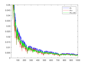
Figure 1: Comparison of $\varphi_{3},\varphi_{3,\pi}$ and $\varphi_{3,\pi,1,000}$ up to $N=1,000$.

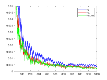
Figure 2: Comparison of $\varphi_{5},\varphi_{5,\pi}$ and $\varphi_{5,\pi,1,000}$ up to $N=1,000$.

Ruhr West University of Applied Sciences, Duisburger Str. 100, D-45479 Mülheim an der Ruhr, christian.weiss@hs-ruhrwest.de

References

- [AL16] C. Aistleitner and G. Larcher. Metric results on the discrepancy of sequences modulo one for integer seuences of polynomial growth. Mathematika, 62(2):478–491, 2016.
- [Ata04] E. I. Atanassov. On the discrepancy of the Halton sequences. Mathematica Balkanica, New Series, 18.1-2:15–32, 2004.
- [Bak81] R. C. Baker. Metric number theory and the large sieve. Journal of the London Mathematical Society, 24 (1):34–40, 1981.
- [BP94] I. Berkes and W. Philipp. The size of trigonometric and Walsh series and uniform distribution mod 1. Journal of the London Mathematical Society, 50 (3):454–464, 1994.
- [BW79] E. Braaten and G. Weller. An improved low-discrepancy sequence for multidimensional quasi-monte carlo integration. Journal of Computational Physics, 33(2):249–258, 1979.
- [CDP23] F. Clément, C. Doerr, and L. Paquete. Heuristic approaches to obtain low-discrepancy point sets via subset selection. arXiv:2306.15276, 2023.
- [CVdN+23] F. Clément, D. Vermetten, J. de Nobel, A. D. Jesus, L. Paquete, and C. C. Doerr. Reproducibility files and additional figures. https://doi.org/10.5281/zenodo.7630260, 2023.
- [CVJ+23] F. Clément, D. Vermetten, J. De Nobeland A. Jesus, L. Paquete, and C. Doerr. Computing star discrepancies with numerical black-box optimization algorithms. In Proceedings of the Genetic and Evolutionary Computation Conference, pages 1330–1338, 2023.
- [DEM96] D.P. Dobkin, D. Eppstein, and D.P. Mitchell. Computing the discrepancy with applications to supersampling patterns. ACM Trans. Graph., 15:354–376, 1996.
- [DGS05] B. Doerr, M. Gnewuch, and A. Srivastav. Bounds and constructions for the star-discrepancy via -covers. Journal of Complexity, 21(5):691–709, 2005.
- [DGW10] B. Doerr, M. Gnewuch, and M. Wahlström. Algorithmic construction of low-discrepancy point sets via dependent randomized rounding. Journal of Complexity, 26(5):490–507, 2010.
- [DGW14] C. Doerr, M. Gnewuch, and M. Wahlström. Calculation of discrepancy measures and applications. In W. Chen, A. Srivastav, and G. Travaglini, editors, A Panorama of Discrepancy Theory, pages 621–678. Springer International Publishing, 2014.
- [DR13] C. Doerr and F.-M. De Rainville. Constructing low star discrepancy point sets with genetic algorithms. In Proceedings of the 15th annual conference on Genetic and evolutionary computation, pages 789–796, 2013.
- [FKP15] H. Faure, P. Kritzer, and F. Pillichshammer. From van der Corput to modern constructions of sequences for quasi-Monte Carlo rules. Indagationes Mathematicae, 26(5):760–822, 2015.
- [GGPP21] A. Gómez, D. Gómez-Pérez, and F. Pillichshammer. Secure pseudorandom bit generators and point sets with low star-discrepancy. Journal of Computational and Applied Mathematics, 396, 2021.
- [Gne08] M. Gnewuch. Bracketing numbers for axis-parallel boxes and applications to geometric discrepancy. Journal of Complexity, 24:154–172, 2008.
- [Gne24] M. Gnewuch. Improved bounds for the bracketing number of orthants or revisiting an algorithm of Thiémard to compute bounds for the star discrepancy. Journal of Complexity, 83, 2024.
- [GPW21] M. Gnewuch, H. Pasing, and C. Weiß. A generalized Faulhaber inequality, improved bracketing covers, and applications to discrepancy. Mathematics of Computation, 332 (90):2873–2898, 2021.
- [GSW09] M. Gnewuch, A. Srivastav, and C. Winzen. Finding optimal volume subintervals with k points and calculating the star discrepancy are NP-hard problems. Journal of Complexity, 25 (2):115–127, 2009.
- [GWW12] M. Gnewuch, M. Wahlström, and C. Winzen. A new randomized algorithm to approximate the star discrepancy based on threshold accepting. SIAM Journal on Numerical Analysis, 50(2):781–807, 2012.
- [HKLP09] R. Hofer, P. Kritzer, G. Larcher, and F. Pillichshammer. Distribution properties of generalized van der Corput–Halton sequences and their subsequences. International Journal of Number Theory, 05(04):719–746, 2009.
- [HNWW00] S. Heinrich, E. Novak, G. Wasilkowski, and H. Wozniakowski. The inverse of the star-discrepancy depends linearly on the dimension. Acta Arithmetica, 96(3):279–302, 2000.
- [KN74] L. Kuipers and H. Niederreiter. Uniform distribution of sequences. John Wiley & Sons, New York, 1974.
- [Mei68] H. G. Meijer. The discrepancy of a g-adic sequence. Indagationes Mathematicae, 30:54–66, 1968.
- [Nie92] H. Niederreiter. Random Number Generation and Quasi-Monte Carlo Methods. Number 63 in CBMS-NSF Series in Applied Mathematics, SIAM, Philadelphia, 1992.
- [NW21] E. Novak and H. Woźniakowski. Tractability of Multivariate problems, volume 2. Eur. Math. Soc. Publ. House, 2021.
- [Ost09] V. Ostromoukhov. Recent progress in improvement of extreme discrepancy and star discrepancy of one-dimensional sequences. In Pierre L’ Ecuyer and Art B. Owen, editors, Monte Carlo and Quasi-Monte Carlo Methods 2008, pages 561–572. Springer Berlin Heidelberg, 2009.
- [Pil12] F. Pillichshammer. On the discrepancy of the van der Corput sequence indexed by Fibonacci numbers. Fibonacci Quaterly, 50 (3):235–238, 2012.
- [RKB+24] T. K. Rusch, N. Kirk, M. Bronstein, C. Lemieux, and D. Rus. Message-passing Monte Carlo: Generating low-discrepancy point sets via graph neural networks. Proceedings of the National Academy of Sciences, 121(40):e2409913121, 2024.
- [Rot54] K. F. Roth. On irregularities of distrubtion. Mathematika, 1:73–79, 1954.
- [Sch72] W. M. Schmidt. Irregularities of distribution vii. Acta Arith., 21:45–50, 1972.
- [Wei24] C. Weiß. Polynomial p-adic low-discrepancy sequences. arXiv:2406.09114, 2024.
- [WN19] C. Weiß and Z. Nikolic. An aspect of optimal regression design for LSMC. Monte Carlo Methods and Applications, 25(4):283–290, 2019.
- [WF97] P. Winker and K.-T. Fang. Application of threshold-accepting to the evaluation of the discrepancy of a set of points. SIAM Journal on Numerical Analysis, 34(5):2028–2042, 1997.