Anisotropic Field Theory of Wave Transmission Statistics in Disordered Media

Abstract

We present a field theory to characterize the mean distribution of transmission eigenvalues for coherent wave propagation through a disordered medium. Unlike the Dorokhov-Mello-Pereyra-Kumar (DMPK) theory, our approach does not rely on the isotropy hypothesis, which assumes uniform field intensity across scattering channels. As a result, it accurately predicts the transmission eigenvalue distribution both in the diffusive and quasiballistic regime. In addition, it proves to be more versatile than the DMPK theory, allowing for the incorporation of physical effects such as absorption or partial channel control with minimal adjustments to the formalism. Although these effects are commonly encountered in experiments on complex media, until now there has been no ab initio theory addressing them. Our predictions are numerically validated against transmission eigenvalue distributions computed from the microscopic wave equation.

Coherent wave propagation in disordered media arises across various fields of science and technology, from optical and acoustic imaging to studies of coherent electron transport in mesoscopic conductors [1, 2, 3]. In many situations it is relevant to describe this propagation using the transmission coefficient matrix, $\mathsf{t}$, which connects the wavefronts at the system input to the wavefronts at the output. The eigenvalues of $\mathsf{t}^{\dagger}\mathsf{t}$, always contained between $0$ and $1$, determine the transmittances of the corresponding eigenmodes. It has been known for decades that, in the diffusive regime, the distribution of these eigenvalues follows the bimodal law, $\rho(T)=\bar{T}/(2T\sqrt{1-T})$, $\bar{T}$ being the mean transmission [4, 5, 6, 7]. Surprisingly, this distribution allows the existence of quasitransparent channels (near $T=1$) despite the on-average opacity of the disordered medium ($\bar{T}\ll 1$). This rather unusual property shows that the incident wavefront can be shaped to minimize the impact of scattering.

The theoretical study of wave transmission through disordered systems was marked by the parallel development of two competing theories: the nonlinear sigma model [8, 9, 10, 11, 12, 13, 14, 15], and the Dorokhov-Mello-Pereyra-Kumar (DMPK) theory [16, 17, 18, 19, 7]. The nonlinear sigma model, on one hand, refers to a class of field-theoretical models defined by constraining the field to a specific target manifold. These models are typically obtained by a systematic approach for averaging over the disorder initially proposed by Wegner and Schäfer [8, 9] and previous authors [20, 21, 22, 23] in the framework of electron transport. This approach originally exploited the replica method to achieve the disorder averaging but was soon endowed of a supersymmetric space by Efetov [10, 11, 12, 13] to avoid the use of replicas. In the following years, many authors used the supersymmetric method to study the transport properties of waves in disordered media especially in the strongly localized regime [24, 25, 26, 27, 28, 29, 30, 31, 32]. Nazarov was the first to derive the transmission eigenvalue distribution in the nonlocalized diffusive regime using a nonlinear sigma model without supersymmetry [33, 34]. His approach, apparently unrelated to that of Efetov, is based on an analogy with kinetic equations for type-II superconductors [35, 36, 37, 38, *Larkin1973, *Larkin1975, *Larkin1977, 42] where the disorder caused by impurities is known to play an important role. Nazarov’s approach did not gain widespread adoption in the literature on disordered systems, probably due to shortcuts in mathematical reasoning. However, given its universality, this approach holds potential applications beyond electron transport, including fields like optics and acoustics. The primary challenge lies in extending the approach to account for quasiballistic transport, absorption, and incomplete channel control—regimes that Nazarov’s method originally did not address.

The DMPK theory, on the other hand, proceeds very differently. It is based on a perturbative treatment of an infinitesimal slice of disordered medium. This approach provides a Fokker-Planck-type equation, known as the DMPK equation, for the joint distribution of transmission eigenvalues. The DMPK theory became very successful for the simplicity, elegance, and predictive power of its formalism [7]. However, it has notable limitations in scenarios of high experimental interest.

A first limitation of the DMPK approach comes from the isotropy hypothesis [17, 7] which assumes that the field intensity is uniformly distributed across the different channels due to scattering by each infinitesimal slice of the disordered medium. It turns out that this isotropy hypothesis is only valid in the multiple-scattering regime and not in the quasiballistic regime. This distorts the predictions of the DMPK theory in the quasiballistic regime, which is experimentally highly relevant. Incidentally, nonlinear sigma models face the same limitation due to the equivalence between the two theories [43, 44, 45]. Another limitation of the DMPK theory reported by Brouwer [46] comes from the inherent difficulties in including absorption, a crucial phenomenon in optics and acoustics. Last but not least, the DMPK theory is focused on the transmission matrix and cannot be modified to study the statistics of other observables such as the field intensity inside the system for example [47, 48], or to account for typical experimental configurations such as partial channel control which results from the limited numerical aperture of measuring devices or the finite spatial extent of the incident beam [49, 50, 51]. All these limitations of the DMPK theory can be overcome by the anisotropic field theory presented in this Letter and derived in the companion paper [52].

To set the framework of our approach, we consider a disordered region of thickness $L$, characterized by the random potential $U(\boldsymbol{\mathrm{r}})$, contained within a perfect waveguide. We assume that the wave is emitted in the transverse mode $\chi_{n}(\boldsymbol{\mathrm{y}})$ from a fictitious surface with longitudinal coordinate $x_{\mathrm{a}}$ and measured in the mode $\chi_{m}(\boldsymbol{\mathrm{y}})$ at another surface at $x_{\mathrm{b}}$. It is not necessary that these surfaces lie outside the disordered region [33, 52]. The transmission matrix coefficient $t_{mn}$ is then determined by the Fisher and Lee relation [53, 54, 55],

$$t_{mn}=2\mathrm{i}\sqrt{k_{x,m}k_{x,n}}\left\langle\chi_{m},x_{\mathrm{b}}\right|\hat{G}^{+}\left|\chi_{n},x_{\mathrm{a}}\right\rangle\>,$$ (1)

where $k_{x,n}$ is the longitudinal wavenumber of mode $n$. In Eq. (1) and those that follow, we use Dirac’s notation: hats denote operators acting in the position space. The waveguide supports $N_{\rm p}$ propagating modes, but only $N_{\mathrm{a}}$ of them are controlled at the input, and $N_{\mathrm{b}}$ at the output. Therefore, the dimensions of $\mathsf{t}$ are $N_{\mathrm{b}}\times N_{\mathrm{a}}$. In Eq. (1), $\hat{G}^{+}$ is the Green’s operator defined by

$$\hat{G}^{\pm}=\big{[}\hat{\nabla}^{2}_{\boldsymbol{\mathrm{r}}}+k^{2}\pm\mathrm{i}\varepsilon-U(\hat{\boldsymbol{\mathrm{r}}})\big{]}^{-1}\>,$$ (2)

where $k=2\pi/\lambda$ is the wavenumber, and $\varepsilon$ the Laplace variable associated with time ($\partial_{t}\leftrightarrow\varepsilon$). The random potential $U(\boldsymbol{\mathrm{r}})$ in Eq. (2) is normally distributed according to $\textstyle\mathcal{P}[U(\boldsymbol{\mathrm{r}})]\propto\exp(-\int_{\mathbb{R}^{d}}\mathop{}\!\mathrm{d}\boldsymbol{\mathrm{r}}\frac{U(\boldsymbol{\mathrm{r}})^{2}}{2\alpha(\boldsymbol{\mathrm{r}})})$. The disorder strength $\alpha$ determines the value of the scattering mean free path, $\ell_{\rm s}=k/\pi\nu\alpha$, where $\nu$ is the local density of states per unit $k^{2}$.

The central quantity is the distribution of transmission eigenvalues defined by

$$\rho(T)\overset{\mathrm{def}}{=}\frac{1}{N_{\mathrm{a}}}\left\langle\operatorname{Tr}\delta(T-\mathsf{t}^{\dagger}\mathsf{t})\right\rangle=\frac{1}{\pi T^{2}}\operatorname{Im}F(\tfrac{1}{T}+0\mathrm{i})\>,$$ (3)

where $\left\langle\cdot\right\rangle$ denotes the average over the random potential $U(\boldsymbol{\mathrm{r}})$. As indicated by the second equality of Eq. (3), the distribution $\rho(T)$ can be extracted from the generating function:

$$F(\gamma)=\frac{1}{N_{\mathrm{a}}}\frac{\mathop{}\!\mathrm{d}}{\mathop{}\!\mathrm{d}\gamma}\left\langle\ln Z(\gamma)\right\rangle\>,$$ (4)

where $Z(\gamma)=\mathcal{N}\det(1-\gamma\mathsf{t}^{\dagger}\mathsf{t})^{-1}$, with $\mathcal{N}$ a $\gamma$-independent arbitrary prefactor. It is useful to write this partition function in the form (see Sec. II B of the companion paper [52]):

$$\begin{split}Z(\gamma)&=\mathcal{N}\det(1-\gamma\hat{G}^{+}\hat{K}_{\mathrm{a}}\hat{G}^{-}\hat{K}_{\mathrm{b}})^{-1}\\ &=\int\mathcal{D}[\boldsymbol{\mathrm{\phi}}(\boldsymbol{\mathrm{r}})]\mathop{}\!\mathrm{e}^{\mathrm{i}\int\mathop{}\!\mathrm{d}\boldsymbol{\mathrm{r}}\>\boldsymbol{\mathrm{\phi}}^{\dagger}(\boldsymbol{\mathrm{r}})[\hat{\mathsf{W}}_{0}-U(\boldsymbol{\mathrm{r}})]\boldsymbol{\mathrm{\phi}}(\boldsymbol{\mathrm{r}})}\>,\end{split}$$ (5)

where $\boldsymbol{\mathrm{\phi}}(\boldsymbol{\mathrm{r}})={[\phi_{1}(\boldsymbol{\mathrm{r}}),\phi_{2}(\boldsymbol{\mathrm{r}})]}^{\intercal}$ is a fictitious two-component complex field, and $\hat{\mathsf{W}}_{0}$ is the disorder-free matrix Hamiltonian

$$\hat{\mathsf{W}}_{0}=\begin{pmatrix}\hat{\nabla}^{2}_{\boldsymbol{\mathrm{r}}}+k^{2}+\mathrm{i}\varepsilon&\gamma\hat{K}_{\mathrm{a}}\\ \hat{K}_{\mathrm{b}}&\hat{\nabla}^{2}_{\boldsymbol{\mathrm{r}}}+k^{2}-\mathrm{i}\varepsilon\end{pmatrix}\>,$$ (6)

$\hat{K}_{\mathrm{a}}$ being a current density operator defined by

$$\hat{K}_{\mathrm{a}}=-\hat{\Theta}_{\mathrm{a}}\mathrm{i}\hat{\nabla}_{x}\delta(\hat{x}-x_{\mathrm{a}})-\delta(\hat{x}-x_{\mathrm{a}})\hat{\Theta}_{\mathrm{a}}\mathrm{i}\hat{\nabla}_{x}\>,$$ (7)

where $\hat{\Theta}_{\mathrm{a}}=\Theta(m_{\mathrm{a}}-\|\hat{\boldsymbol{\mathrm{\Omega}}}_{\perp}\|)$ with $\hat{\boldsymbol{\mathrm{\Omega}}}_{\perp}=\tfrac{1}{\mathrm{i}k}\hat{\boldsymbol{\mathrm{\nabla}}}_{\boldsymbol{\mathrm{y}}}$, and similarly for $\hat{K}_{\mathrm{b}}$. The Heaviside step function $\Theta$ has the effect of reducing the number of modes under control when $m_{\mathrm{a}}<1$ or $m_{\mathrm{b}}<1$. The parameters $m_{\mathrm{a}}$ and $m_{\mathrm{b}}$ are the numerical apertures of the input and output ports, respectively. In two dimensions, they are given by $m_{\mathrm{a}}=N_{\mathrm{a}}/N_{\rm p}$ and $m_{\mathrm{b}}=N_{\mathrm{b}}/N_{\rm p}$ [49].

The average over the disorder in Eq. (4) can be calculated by the standard replica method [14], $\textstyle\left\langle\ln Z\right\rangle=\lim_{R\rightarrow 0}\partial_{R}\left\langle Z^{R}\right\rangle$, where $R$ is the number of replicas. Introducing the replicated field, denoted as $\boldsymbol{\mathrm{\Phi}}(\boldsymbol{\mathrm{r}})={[\boldsymbol{\mathrm{\phi}}_{1}(\boldsymbol{\mathrm{r}}),\ldots,\boldsymbol{\mathrm{\phi}}_{R}(\boldsymbol{\mathrm{r}})]}^{\intercal}$, yields

$$\left\langle Z^{R}\right\rangle=\int\mathcal{D}[U]\mathcal{D}[\boldsymbol{\mathrm{\Phi}}]\mathop{}\!\mathrm{e}^{\int\mathop{}\!\mathrm{d}\boldsymbol{\mathrm{r}}\left(-\frac{U^{2}}{2\alpha}+\mathrm{i}\boldsymbol{\mathrm{\Phi}}^{\dagger}(\hat{\mathsf{W}}_{0}-U)\boldsymbol{\mathrm{\Phi}}\right)}\>.$$ (8)

The integral over $U(\boldsymbol{\mathrm{r}})$ being Gaussian, we get

$$\left\langle Z^{R}\right\rangle=\int\mathcal{D}[\boldsymbol{\mathrm{\Phi}}]\mathop{}\!\mathrm{e}^{\int\mathop{}\!\mathrm{d}\boldsymbol{\mathrm{r}}\left(\mathrm{i}\boldsymbol{\mathrm{\Phi}}^{\dagger}\hat{\mathsf{W}}_{0}\boldsymbol{\mathrm{\Phi}}-\frac{\alpha}{2}(\boldsymbol{\mathrm{\Phi}}^{\dagger}\boldsymbol{\mathrm{\Phi}})^{2}\right)}\>.$$ (9)

The Lagrangian in the exponential argument possesses a $\boldsymbol{\mathrm{\Phi}}^{4}$ term giving rise to Goldstone modes at the saddle points [9]. Since these modes vary in position space much more slowly than the wavelength, they can be approximated semiclassically as we will see shortly. The $\boldsymbol{\mathrm{\Phi}}^{4}$ term can be eliminated by a Hubbard-Stratonovich transformation [13] which consists in the introduction of an auxiliary matrix field of dimensions $2R\times 2R$ denoted $\mathsf{Q}(\boldsymbol{\mathrm{r}})$:

$$\left\langle Z^{R}\right\rangle=\int\mathcal{D}[\mathsf{Q}]\mathop{}\!\mathrm{e}^{\int\mathop{}\!\mathrm{d}\boldsymbol{\mathrm{r}}\left(\frac{\alpha}{2}\operatorname{Tr}[\mathsf{Q}(\boldsymbol{\mathrm{r}})^{2}]-\left\langle\boldsymbol{\mathrm{r}}\right|\operatorname{Tr}\ln(\hat{\mathsf{W}}_{0}+\mathrm{i}\alpha\mathsf{Q}(\hat{\boldsymbol{\mathrm{r}}}))\left|\boldsymbol{\mathrm{r}}\right\rangle\right)}\>.$$ (10)

It is possible to simplify the Lagrangian in Eq. (10) by assuming the diffusive regime ($L\gg\ell_{\rm s}$). This would lead to a nonlinear sigma model. However, we do not make this assumption because it is equivalent to the isotropy hypothesis and is approximate. Instead, we consider the saddle-point equation of the Lagrangian in Eq. (10), which has the form of a nonlinear wave equation for the matrix Green’s function $\mathsf{\Gamma}(\boldsymbol{\mathrm{r}},\boldsymbol{\mathrm{r}}^{\prime})$,

$$\begin{split}\Big{[}&\nabla^{2}_{\boldsymbol{\mathrm{r}}}+k^{2}+\mathrm{i}\varepsilon\mathsf{\Lambda}_{3}+\mathrm{i}\alpha\mathsf{Q}(\boldsymbol{\mathrm{r}})\\ &+\gamma_{\mathrm{a}}\hat{K}_{\mathrm{a}}\mathsf{\Lambda}_{+}+\gamma_{\mathrm{b}}\hat{K}_{\mathrm{b}}\mathsf{\Lambda}_{-}\Big{]}\mathsf{\Gamma}(\boldsymbol{\mathrm{r}},\boldsymbol{\mathrm{r}}^{\prime})=\mathrm{i}\mathsf{1}_{2}\delta(\boldsymbol{\mathrm{r}}-\boldsymbol{\mathrm{r}}^{\prime})\>,\end{split}$$ (11)

with the self-consistency condition $\mathsf{Q}(\boldsymbol{\mathrm{r}})=\mathsf{\Gamma}(\boldsymbol{\mathrm{r}},\boldsymbol{\mathrm{r}})$ and the Pauli matrices $\mathsf{\Lambda}_{1,2,3,\pm}$. As explained in the companion paper [52], the saddle-point approximation is well justified in the nonlocalized regime ($L\ll\xi$, where $\xi$ is the localization length). Additionally, coupling between replicas can be neglected in this regime. This allows us to approximate $\left\langle Z^{R}\right\rangle\simeq\bar{Z}^{R}$ where $\bar{Z}$ is the partition function (10) corresponding to a single replica ($R=1$). Since the problem is reduced to one replica, the field $\mathsf{Q}(\boldsymbol{\mathrm{r}})$ becomes a $2\times 2$ matrix. After this simplification, it is relevant to approximate Eq. (11) semiclassically using the Wigner transform. In this regard, we define the matrix radiance $\mathsf{g}(\boldsymbol{\mathrm{\Omega}},\boldsymbol{\mathrm{r}})$ as

$$\mathsf{g}(\boldsymbol{\mathrm{\Omega}},\boldsymbol{\mathrm{r}})=\frac{2k}{\pi}\mathchoice{{\vbox{\hbox{$\textstyle-$}}\kern-4.86108pt}}{{\vbox{\hbox{$\scriptstyle-$}}\kern-3.25pt}}{{\vbox{\hbox{$\scriptscriptstyle-$}}\kern-2.29166pt}}{{\vbox{\hbox{$\scriptscriptstyle-$}}\kern-1.875pt}}\!\int_{k}\mathop{}\!\mathrm{d}{p}\int_{\mathbb{R}^{d}}\mathop{}\!\mathrm{d}{\boldsymbol{\mathrm{s}}}\>\mathsf{\Gamma}(\boldsymbol{\mathrm{r}}+\tfrac{\boldsymbol{\mathrm{s}}}{2},\boldsymbol{\mathrm{r}}-\tfrac{\boldsymbol{\mathrm{s}}}{2})\mathop{}\!\mathrm{e}^{-\mathrm{i}p\boldsymbol{\mathrm{\Omega}}\cdot\boldsymbol{\mathrm{s}}}\>.$$ (12)

The dashed integral on $p$ in Eq. (12) only retains the Cauchy principal value on the wavenumber shell $\left\|\boldsymbol{\mathrm{p}}\right\|=k$. As shown in Sec. III B of the companion paper [52], the result of the Wigner transform of Eq. (11) is a nonlinear matrix transport equation for $\mathsf{g}(\boldsymbol{\mathrm{\Omega}},\boldsymbol{\mathrm{r}})$,

$$\begin{split}\boldsymbol{\mathrm{\Omega}}\cdot\boldsymbol{\mathrm{\nabla}}_{\boldsymbol{\mathrm{r}}}\mathsf{g}=&-\tfrac{1}{2\ell_{\rm s}}[\tilde{\mathsf{Q}}(\boldsymbol{\mathrm{r}}),\mathsf{g}]-\tfrac{\varepsilon}{2k}[\mathsf{\Lambda}_{3},\mathsf{g}]\\ &+\mathrm{i}\gamma\Omega_{x}\Theta(m_{\mathrm{a}}-\left\|\boldsymbol{\mathrm{\Omega}}_{\perp}\right\|)\delta(x-x_{\mathrm{a}})[\mathsf{\Lambda}_{+},\mathsf{g}]\\ &+\mathrm{i}\Omega_{x}\Theta(m_{\mathrm{b}}-\left\|\boldsymbol{\mathrm{\Omega}}_{\perp}\right\|)\delta(x-x_{\mathrm{b}})[\mathsf{\Lambda}_{-},\mathsf{g}]\>,\end{split}$$ (13)

reminiscent of the Eilenberger equation from the superconductivity literature [37, 38, *Larkin1973, *Larkin1975, *Larkin1977, 42, 56, 57, 34]. In Eq. (13), $[\mathsf{A},\mathsf{B}]=\mathsf{A}\mathsf{B}-\mathsf{B}\mathsf{A}$ is the commutator and $\tilde{\mathsf{Q}}(\boldsymbol{\mathrm{r}})$ is the normalized field:

$$\tilde{\mathsf{Q}}(\boldsymbol{\mathrm{r}})\overset{\mathrm{def}}{=}\frac{1}{\pi\nu}\mathsf{Q}(\boldsymbol{\mathrm{r}})=\oint\frac{\mathop{}\!\mathrm{d}\boldsymbol{\mathrm{\Omega}}}{S_{d}}\mathsf{g}(\boldsymbol{\mathrm{\Omega}},\boldsymbol{\mathrm{r}})\>,$$ (14)

$S_{d}$ being the surface area of the unit $d$-ball.

Equation (13) must be completed by appropriate boundary conditions that can be extracted from the asymptotic behavior of $\mathsf{g}(\boldsymbol{\mathrm{\Omega}},\boldsymbol{\mathrm{r}})$ prescribed by Eqs. (11)–(12) for $\boldsymbol{\mathrm{r}}\rightarrow\infty$. We show in Sec. III C of the companion paper [52] that

$$\mathsf{g}_{\rm out}(\boldsymbol{\mathrm{\Omega}},\boldsymbol{\mathrm{r}})=\begin{pmatrix}1&g_{12}\\ 0&-1\end{pmatrix}\>,\quad\mathsf{g}_{\rm in}(\boldsymbol{\mathrm{\Omega}},\boldsymbol{\mathrm{r}})=\begin{pmatrix}1&0\\ g_{21}&-1\end{pmatrix}\>.$$ (15)

The indices “in” and “out” denote the incoming and outgoing directions $\boldsymbol{\mathrm{\Omega}}$ on the disordered region, respectively. Note that Eq. (15) fixes only three elements of the matrix $\mathsf{g}$ out of four. The remaining elements $g_{12}$ and $g_{21}$ are free. As Eq. (13) satisfies the properties $\boldsymbol{\mathrm{\nabla}}_{\boldsymbol{\mathrm{r}}}\left[\mathsf{g}(\boldsymbol{\mathrm{\Omega}},\boldsymbol{\mathrm{r}})^{2}\right]=\boldsymbol{\mathrm{\mathsf{0}}}$ and $\boldsymbol{\mathrm{\nabla}}_{\boldsymbol{\mathrm{r}}}\operatorname{Tr}\mathsf{g}(\boldsymbol{\mathrm{\Omega}},\boldsymbol{\mathrm{r}})=\boldsymbol{\mathrm{0}}$, the boundary conditions (15) impose the following important constraints:

$$\mathsf{g}(\boldsymbol{\mathrm{\Omega}},\boldsymbol{\mathrm{r}})^{2}=\mathsf{1}\>,\quad\operatorname{Tr}\mathsf{g}(\boldsymbol{\mathrm{\Omega}},\boldsymbol{\mathrm{r}})=0\>,\quad\forall\,\boldsymbol{\mathrm{\Omega}},\boldsymbol{\mathrm{r}}\>.$$ (16)

It is worth noting that the property $\mathsf{g}^{2}=\mathsf{1}$ is more general than the normalization $\tilde{\mathsf{Q}}^{2}=\mathsf{1}$ in nonlinear sigma models, which holds only in the isotropic limit due to the relationship given in Eq. (14). Once the system of equations (13)–(15) is solved, the generating function (4) can be calculated with:

$$F(\gamma)=\mathrm{i}\int_{\left\|\boldsymbol{\mathrm{\Omega}}_{\perp}\right\|\leq m_{\mathrm{a}}}\frac{\mathop{}\!\mathrm{d}\boldsymbol{\mathrm{\Omega}}\>\Omega_{x}}{2V_{d-1}}\operatorname{Tr}[\mathsf{g}(\boldsymbol{\mathrm{\Omega}},x_{\mathrm{a}})\mathsf{\Lambda}_{+}]\>,$$ (17)

$V_{d}$ being the volume of the unit $d$-ball.

Now, we numerically investigate the validity of the theory (13)–(17) in a two-dimensional waveguide ($d=2$) of transverse width $W$. We assume that the transverse boundary conditions are periodic [$\chi_{n}(y+W)=\chi_{n}(y)$]. This assumption aims at making the field $\mathsf{Q}(x,y)$ independent of $y$ in order to simplify the numerical procedures. Of course, the theory remains perfectly valid for Dirichlet boundary conditions if we let $\mathsf{Q}(x,y)$ vary in $y$ to vanish at the boundaries. We verified that the impact of boundary conditions is marginal in quasiballistic and diffusive regimes. The two equations (13) and (14) are solved iteratively until self-consistency is achieved. The integration of Eq. (13) along $x$ under the constraints (16) can be carried out by means of the parametrization $\mathsf{g}(\boldsymbol{\mathrm{\Omega}},\boldsymbol{\mathrm{r}})=\mathsf{M}(\boldsymbol{\mathrm{\Omega}},\boldsymbol{\mathrm{r}})\mathsf{\Lambda}_{3}\mathsf{M}(\boldsymbol{\mathrm{\Omega}},\boldsymbol{\mathrm{r}})^{-1}$ where $\mathsf{M}$ is an arbitrary matrix with two independent parameters. See the companion paper [52] for further details on the numerical integration of Eq. (13).

Our theoretical predictions are compared to transmission eigenvalue distributions computed numerically via the recursive Green’s function method, applied to the microscopic wave equation associated with Eq. (2), and averaged over disorder realizations.

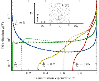
Figure 1: Transmission eigenvalue distribution for a disordered waveguide with $W/\lambda=50.5$, $L/W=1$, and $m_{\mathrm{a}}=m_{\mathrm{b}}=1$, at different optical thicknesses $L/\ell_{\rm s}$. Numerical distributions (dots) are computed from the microscopic wave equation and averaged over $5\times 10^{4}$ disorder realizations, and compared to the predictions from the field theory (13)–(17) (solid) and the DMPK theory (dashed).

As can be seen in Fig. 1, the theory (13)–(17) (solid lines) agrees with numerical distributions (dots), including in the quasiballistic regime ($L\lesssim\ell_{\rm s}$). The marked deviations of the DMPK theory [16, 17, 7] (dashed lines) in the region $T<1$ arise solely from the approximate nature of the isotropy hypothesis. This hypothesis is only valid in diffusive regime ($L\gg\ell_{\rm s}$) where the bimodal law applies (see Fig. 1 for $L/\ell_{\rm s}=5$).

It is worth noting that the isotropy hypothesis can be implemented in the matrix transport equation (13) by setting

$$\mathsf{g}(\boldsymbol{\mathrm{\Omega}},\boldsymbol{\mathrm{r}})=\tilde{\mathsf{Q}}(\boldsymbol{\mathrm{r}})+\boldsymbol{\mathrm{\Omega}}\cdot\tilde{\boldsymbol{\mathrm{\mathsf{J}}}}(\boldsymbol{\mathrm{r}})\>,$$ (18)

where $\tilde{\boldsymbol{\mathrm{\mathsf{J}}}}(\boldsymbol{\mathrm{r}})$ is a matrix current (a vector of matrices), and assuming that $\|\tilde{\boldsymbol{\mathrm{\mathsf{J}}}}\|\ll\|\tilde{\mathsf{Q}}\|$, as done in the diffusion approximation. This approach leads to a Usadel-type equation [42, 33, 34], a nonlinear matrix diffusion equation closed for $\tilde{\mathsf{Q}}(\boldsymbol{\mathrm{r}})$. This equation can also be derived from the saddle-point equation of a nonlinear sigma model [14, 34, 57, 15] and matches the DMPK solution in the absence of absorption [43, 44, 45].

Additionally, Eq. (13) can be solved in the quasiballistic regime ($L\lesssim\ell_{\rm s}$), where the field $\tilde{\mathsf{Q}}(\boldsymbol{\mathrm{r}})$ is nearly constant within the disordered region. This approximation serves as the dual to the isotropy hypothesis in DMPK theory: it approximates position space while treating direction space exactly, whereas DMPK does the reverse. As shown in Sec. III D of the companion paper [52], this approximation leads to a self-consistent equation for $f(\boldsymbol{\mathrm{\Omega}})$,

$$f(\boldsymbol{\mathrm{\Omega}})=\frac{1-\left(1-\bar{f}\right)\frac{1}{\sigma}\tanh(\frac{L\sigma}{2\ell_{\rm s}\Omega_{x}})}{1+\left(1+\frac{\gamma}{1-\gamma}\bar{f}\right)\frac{1}{\sigma}\tanh(\frac{L\sigma}{2\ell_{\rm s}\Omega_{x}})}\>,$$ (19)

where $\sigma$ and the directional average $\bar{f}$ are defined by

$$\sigma=\sqrt{1+\frac{\gamma\bar{f}^{2}}{1-\gamma}}\>,\quad\bar{f}=\int_{\Omega_{x}>0}\frac{\mathop{}\!\mathrm{d}{\boldsymbol{\mathrm{\Omega}}}}{\frac{1}{2}S_{d}}\>f(\boldsymbol{\mathrm{\Omega}})\>.$$ (20)

The sought generating function is then given by inserting $\mathsf{g}(\boldsymbol{\mathrm{\Omega}})=\tfrac{-2\mathrm{i}}{1-\gamma}f(\boldsymbol{\mathrm{\Omega}})\Theta(\Omega_{x})\mathsf{\Lambda}_{-}$ into Eq. (17). The solution of Eqs. (19)–(20) is significantly more accurate than the DMPK theory in the quasiballistic regime (see Figs. 4–5 of the companion paper [52]).

Apart from its accuracy in the quasiballistic regime, another advantage of Eq. (13) is its ability to directly incorporate the effect of absorption in the medium by redefining the parameter $\varepsilon$ as $\varepsilon=k/\ell_{\rm a}$, where $\ell_{\rm a}$ denotes the ballistic absorption length. In Fig. 2 we compare the predictions of the full model (13) (solid lines) and its isotropic version based on Eq. (18) (dashed lines) with results from numerical simulations (dots).

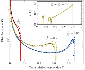
Figure 2: Transmission eigenvalue distribution for an absorbing disordered waveguide with $W/\lambda=50.5$, $L/W=1$, $L/\ell_{\rm s}=5$, and $m_{\mathrm{a}}=m_{\mathrm{b}}=1$, shown for different absorption lengths $\ell_{\rm a}$. Numerical distributions (dots) are compared with predictions from the anisotropic field theory (13)–(17) (solid) and its isotropic version based on Eq. (18) (dashed). The inset displays the distribution for $L/\ell_{\rm s}=L/\ell_{\rm a}=0.2$, with the corresponding numerical distribution shown as dotted line.

Interestingly, we find that absorption tends to break the isotropy of $\mathsf{g}$, even in the diffusive regime ($L/\ell_{\rm s}=5$ in Fig. 2), owing to the variation in average path lengths taken by incoming waves based on their angle of incidence. This deviation disappears for $L/\ell_{\rm s}\gg 10$. In the quasiballistic regime, lobes become visible (see inset of Fig. 2), resulting from higher transverse modes which, due to their extended paths in the absorbing medium, contribute to lower transmission. This lobe-splitting effect cannot be captured by an isotropic theory. We also emphasize that no theoretical prediction has been available until now for the experimentally relevant regime of moderate absorption, $\ell_{\rm a}\leq L\ll\xi_{\rm a}$, where $\xi_{\rm a}=\sqrt{\ell_{\rm s}\ell_{\rm a}/2}$ denotes the diffusive absorption length. The approximation proposed in Ref. [46] applies only in the strongly absorbing regime, $L\gg\xi_{\rm a}$, where transmission is minimal.

Finally, we consider an experimental situation where only modes within the input port’s numerical aperture $m_{\mathrm{a}}$ (i.e., $\left\|\boldsymbol{\mathrm{\Omega}}_{\perp}\right\|\leq m_{\mathrm{a}}$) are injected. At the outport port, we assume that all waveguide modes are accessible ($m_{\mathrm{b}}=1$), making the transmission matrix $\mathsf{t}$ rectangular with more rows than columns.

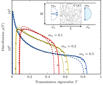
Figure 3: Transmission eigenvalue distribution for a disordered waveguide with $W/\lambda=50.5$, $L/W=1$, $L/\ell_{\rm s}=5$, and $L/\ell_{\rm a}=0$, shown for different input port numerical apertures $m_{\mathrm{a}}$. The output port has maximum numerical aperture ($m_{\mathrm{b}}=1$). Numerical distributions (dots) are compared with the predictions from the field theory (13)–(17) (solid) and FRM theory [49] with $\bar{T}=1/(1+\tfrac{2L}{\pi\ell_{\rm s}})\simeq 0.239$ (dashed).

The distributions obtained in this case are compared in Fig. 3 with the predictions of filtered random matrix (FRM) theory [49], in a regime of moderate optical thickness, where the FRM model is known to be imperfect. Once again, our new formalism provides a better fit to the observed distributions. In principle, Eq. (13) could also be extended to account for the effects of lateral diffusion in open geometries, avoiding the need for nontrivial renormalization of the FRM parameters in terms of long-range correlations [50, 51].

In conclusion, this Letter introduces an anisotropic field framework for the transmission eigenvalue distribution in disordered media. The core of this approach is the self-consistent matrix transport equation (13), which allows us to predict the correct distribution in the quasiballistic regime—a novel achievement, building on prior work [33, 57, 34] inspired by superconductivity [37, 38, *Larkin1973, *Larkin1975, *Larkin1977, 42]. Our model also rigorously accommodates medium absorption and practical measurement setups. Because of its flexibility, this framework opens up new avenues: it can describe incident beams with finite spatial extent [50, 51], statistics of observables beyond transmission, such as internal field intensity [47, 48], and is adaptable to non-rectilinear geometries [58]. Furthermore, due to its microscopic foundation, it can be extended to capture effects such as anisotropic scattering in biological tissues or the impact of correlated disorder [59]. We anticipate significant breakthroughs in understanding wave propagation in complex media through this approach.