Dynamics of Quantum Correlations and Entanglement Generation in Electron-Molecule Inelastic Scattering.

Abstract

The dynamics and processes involved in particle-molecule scattering, including nuclear dynamics, is described and analyzed by different quantum information quantities along the different stages of the scattering. The main process studied and characterized with the information quantities is the interatomic coulombic electronic capture (ICEC), an inelastic process that can lead to dissociation of the target molecule. The analysis is focused in a one-dimensional transversely confined NeHe molecule model used to simulate the scattering between an electron $\text{e}^{-}$(particle) and a $\text{NeHe}^{+}$ ion (molecule). The time-independent Schrödinger equation (TISE) is solved using the Finite Element Method (FEM) with a self-developed Julia package FEMTISE to compute potential energy curves (PECs) and the parameters of the interactions between particles. The time-dependent Schrödinger equation (TDSE) is solved using the Multi-configuration time-dependent Hartree (MCTDH) algorithm. The time dependent electronic and nuclear probability densities are calculated for different electron incoming energies, evidencing elastic and inelastic processes that can be correlated to changes in von Neumann entropy, conditional mutual information and Shannon entropies. The expectation value of the position of the particles, as well as their standard deviations, are analyzed along the whole dynamics and related to the entanglement during the collision and after the process is over, hence evidencing the dynamics of entanglement generation. It is shown that the correlations generated in the collision is partially retained only when the inelastic process is active.

I INTRODUCTION

The study of particle-molecule scattering processes including nuclear degrees of freedom is fundamental to the understanding of chemical reactions, molecular dissociation, particle capture and in photochemistry [1, 2, 3, 4, 5, 6, 7, 8, 9], to name a few fields of application. The interaction between colliding particles and molecular ions, in the low kinetic energy range, up to tens of eVs, offers insight into the internal quantum mechanical behavior and the information transfer between constituents, when they are treated as subsystems. The dynamical behavior of entanglement and correlation measures between these subsystems in charge migration [10], photoexcitation by lasers [11, 9] and nuclear pathways manipulations [3, 8] is of current interest since it delves into the basic physics of transfer and generation of entanglement between subsystems present in femto- and attochemistry. Similar interests are raised also in the capture and emission processes of charge carriers inside low dimensional solid state nanostructures [12, 13].

There is a plethora of possible outcomes from a collision process, from elastic scattering to dissociation mechanisms via excitation of the molecule or its constituent atoms [14, 15, 16, 2, 17, 18, 19, 20, 21]. Inelastic scattering processes have great impact in generating correlations between the different atoms composing the molecule and also with the scattered particle [22]. A theoretically predicted inelastic process, known as interatomic Coulombic electronic capture (ICEC) [17, 21, 23], is of great interest due to its potential to induce molecular dissociation following the capture of an incoming electron. This process exemplifies how particle capture impacts molecular stability if nuclear dynamics is included and provides a simplified model for exploring entanglement dynamics in quantum scattering [22, 24, 25, 26, 12].

In this work, the entanglement and correlations dynamics of a one-dimensional scattering of an electron ($\text{e}^{-}$) with a $\text{NeHe}^{+}$ ion is investigated. The one-dimensional system, derived from first principles, allows to examine ICEC and related phenomena using a rigorous computational approach. The work focuses on characterizing the different scattering stages using quantum information measures, including von Neumann entropy, conditional mutual information, and Shannon entropy [27]. By analyzing the electronic and nuclear probability densities over time for various electron impact energies, the existence of elastic and inelastic processes is made apparent and changes in quantum information metrics are linked to their occurrence. Additionally, the particle positions and standard deviations can be connected to entanglement and correlation increase or decrease throughout the collision process, thus elucidating how they are generated and whether they survive or not after particle-molecule interaction is over.

The work is organized as follows, in Section II the model for the confined NeHe⁺ molecule is introduced, in Section III the selection of the different parameters of the model, the methods used for the computation of the potential energy curves and dynamical simulations, and the quantities used in the analysis of the results are described. In Section IV the description and discussion the results for the different quantities is presented to finally conclude in Section V.

II MODEL DESCRIPTION

In order to describe how the dynamics of a scattering mechanism in a composite system can be tracked using information measures, a one-dimensional model for electron impact on NeHe⁺ is used. The charged molecule is described by two cations, $\text{Ne}^{+}$ and a $\text{He}^{+}$, and one electron that provides the binding between them. The incident electron impinges in the molecule producing elastic and inelastic scattering phenomena which can produce different excitations as well as dissociation of the molecule. It is assumed that the system is under the effect of a transversal harmonic confinement potential and the interactions between the cations and electrons are derived in Sec. II.1. Figure 1 shows a diagram of the system.

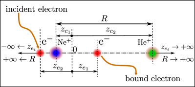
Figure 1: Schematic representation of the coordinates used in the electron-impact model, where an incoming electron collides with a $\text{NeHe}^{+}$ ion. The coordinate $z_{e_{2}}$ denotes the longitudinal position of the incoming electron (projectile), while $z_{e_{1}}$ and $R$ represent the longitudinal position of the bound electron and the internuclear distance of the target, respectively. The spatial arrangement shows the projectile on the left, and the target ion on the right, with the target composed of a Neon cation to the left of nuclei center of mass (CM) and a Helium cation to the right of CM.

The three-dimensional Hamiltonian operator for two electrons and two cations in lateral confinement can be written as,

$$\hat{H}_{\text{tot}}=\hat{T}+\hat{V}_{\text{conf}}+\hat{V}_{\text{int}},$$ (1)

where $\hat{T}$ is the kinetic energy operator, $\hat{V}_{\text{conf}}$ is the confinement potential and $\hat{V}_{\text{int}}$ is the interaction potential. Explicitly each term has the following form,

$$\hat{T}=\sum\nolimits_{i}\hat{T}_{i};\ \hat{V}_{\text{conf}}=\sum\nolimits_{i}\hat{V}_{i};\ \hat{V}_{\text{int}}=\sum\nolimits_{i,j\land i\neq j}\hat{V}_{ij}$$ (2)

were $i,j=\{e_{1},e_{2},c_{1},c_{2}\}$ and $e$ refers to electron particle and $c$ to a cation particle. Each term in Eq. (2) can be further expanded as

$$\hat{T}_{i} = \frac{\mbox{\boldmath${p}$}^{2}_{i}}{2m_{i}}$$ (3)

$$\hat{V}_{i} = \frac{m_{i}(\omega_{i})^{2}}{2}(\mbox{\boldmath${\rho}$}_{i}\cdotp\mbox{\boldmath${\rho}$}_{i})$$ (4)

$$\hat{V}_{ij} = \frac{q_{i}q_{j}\exp(-\alpha_{ij}|\mbox{\boldmath${r}$}_{j}-\mbox{\boldmath${r}$}_{i}|)}{|\mbox{\boldmath${r}$}_{j}-\mbox{\boldmath${r}$}_{i}|}$$ (5)

where $\mbox{\boldmath${r}$}_{i}$ is the position vector and $\mbox{\boldmath${\rho}$}_{i}$ is its polar projection. The expression for $\hat{V}_{i}$ represents a transversal harmonic confinement. The expression for $\hat{V}_{ij}$ represents generic electrostatic Yukawa (Coulomb for $\alpha_{ij}=0$) interactions between a pair of particles with charges $q_{i}$ and $q_{j}$, and specific parameters, defined by $\alpha_{ij}$, which are established as in Sec. III.1.

The Hamiltonian (1) can be rewritten in terms of nuclei center of mass (CM) and relative coordinates $\mbox{\boldmath${r}$}_{\text{CM}}=(\sum_{i=c_{1},c_{2}}m_{i}\mbox{\boldmath${r}$}_{i})/m_{\text{tot}}$ and $\mbox{\boldmath${r}$}_{c_{12}}=|\mbox{\boldmath${r}$}_{c_{1}}-\mbox{\boldmath${r}$}_{c_{2}}|$, respectively. The corresponding masses (total and reduced, in that order) and canonical momenta are $m_{\text{tot}}=(m_{c_{1}}+m_{c_{2}})$, $m_{\text{red}}=m_{c_{1}}m_{c_{2}}/m_{\text{tot}}$ and $\mbox{\boldmath${p}$}_{\text{CM}}=(\mbox{\boldmath${p}$}_{c_{1}}+\mbox{\boldmath${{p}}$}_{c_{2}})$, $\mbox{\boldmath${p}$}_{c_{12}}=(m_{c_{2}}\mbox{\boldmath${p}$}_{c_{1}}-m_{c_{1}}\mbox{\boldmath${p}$}_{c_{2}})/m_{\text{tot}}$. Using this transformation we have,

$$\hat{H}_{\text{tot}}=\hat{T}_{\text{CM}}+\hat{H}_{3D}$$ (6)

where

$$\hat{H}_{\text{3D}}=\hat{T}_{c_{12}}+\hat{T}_{e_{1}}+\hat{T}_{e_{2}}+\hat{V}_{\text{conf}}+\hat{V}_{\text{int}}$$ (7)

is the working Hamiltonian. Note that the vectors $\mbox{\boldmath${r}$}_{e_{i}}-\mbox{\boldmath${r}$}_{c_{j}}$ can be rewritten as,

$$(\mbox{\boldmath${r}$}_{e_{i}}-\mbox{\boldmath${r}$}_{c_{j}}) = \mbox{\boldmath${r}$}_{e_{i}}-\left[\frac{m_{\text{red}}}{m_{c_{j}}}(\mbox{\boldmath${r}$}_{c_{1}}-\mbox{\boldmath${r}$}_{c_{2}})+\mbox{\boldmath${r}$}_{\text{CM}}\right]$$ (8)

$$= \mbox{\boldmath${r}$}_{e_{i}\text{CM}}-\frac{m_{\text{red}}}{m_{c_{j}}}\mbox{\boldmath${r}$}_{c_{12}}$$

where $\mbox{\boldmath${r}$}_{e_{i}\text{CM}}=\mbox{\boldmath${r}$}_{e_{i}}-\mbox{\boldmath${r}$}_{\text{CM}}$ is the coordinate of electron $i$ relative to the center of mass.

II.1 Effective one-dimensional model

If the confinement potential is sufficiently strong (see Sec. III.1) the total wave function can be approximated as

$$\Psi(\mbox{\boldmath${r}$}_{e_{1}},\mbox{\boldmath${r}$}_{e_{2}},\mbox{\boldmath${r}$}_{c_{12}})=\psi(z_{e_{1}},z_{e_{2}},z_{c_{12}})\prod_{i=\{e_{1},e_{2},c_{12}\}}\zeta^{(i)}_{0}(\mbox{\boldmath${\rho}$}_{i})$$ (9)

where $\zeta^{(i)}_{0}(\mbox{\boldmath${\rho}$}_{i})$ are the eigenfunctions of

$$(\hat{T}_{\mbox{\boldmath${\rho}$}_{i}}+\hat{V}_{i})\zeta^{(i)}_{0}(\mbox{\boldmath${\rho}$}_{i})=\hbar\omega_{i}\zeta^{(i)}_{0}(\mbox{\boldmath${\rho}$}_{i})$$ (10)

i.e., the ground state of a two-dimensional isotropic quantum harmonic oscillator, which represents the transversal part of the total wave function and $\psi(z_{e_{1}},z_{e_{2}},z_{c_{12}})$ is a one dimensional wave function (in each coordinate) representing a longitudinal part of the total wave function. The oscillator frequencies $\omega_{i}$ are set up considering a fixed confinement length size $l_{c}$ for all the particles.

The interaction energy between particles $k$ and $l$ can be expressed by the following integral,

$$\left\langle\Psi|\hat{V}_{kl}|\Psi\right\rangle=\iiint\|\psi(z_{e_{1}},z_{e_{2}},z_{c_{12}})\|^{2}V^{(kl)}_{\text{eff}}(|z_{kl}|)\prod_{i}dz_{i}$$ (11)

where $V^{(kl)}_{\text{eff}}(|z|)=\iiint|\zeta^{(i)}_{0}(\mbox{\boldmath${\rho}$}_{i})|^{2}V_{kl}(|\mbox{\boldmath${r}$}|)\prod_{i}d\mbox{\boldmath${\rho}$}_{i}$. As is shown in Eq. (11), the interaction potential is expressed as the integral of the longitudinal wave function times an effective one dimensional potential energy $\hat{V}^{(kl)}_{\text{eff}}$ [28, 13]. A similar result is obtained for all the terms in the Hamiltonian (7), hence the following one dimensional effective Hamiltonian is obtained,

$$\hat{H}=\sum_{i}(\hat{T}_{z_{i}}+\hbar\omega_{i})+\hat{V}_{\text{eff}},$$ (12)

where $\hat{V}_{\text{eff}}=\sum_{k\neq l}\hat{V}^{(kl)}_{\text{eff}}$. The effective interaction potentials $\hat{V}^{(kl)}_{\text{eff}}$ are analytically obtained for each pair of particles [29],

$$V_{\text{eff}}^{(kl)}(z) = \frac{\pi^{\frac{3}{2}}q_{k}q_{l}}{2\left(\sqrt{2}l_{c}\right)}\text{exp}\left[\left(\frac{|z|}{\sqrt{2}l_{c}}\right)^{2}+\left(\frac{\sqrt{2}l_{c}}{2l_{\alpha_{kl}}}\right)^{2}\right]\times$$ (13)

$$\times\text{erfc}\left[\mathnormal{\frac{|z|}{\sqrt{2}l_{c}}+\frac{\sqrt{2}l_{c}}{2l_{\alpha_{kl}}}}\right],$$

where $q_{k}$ is the effective charge, $l_{\alpha_{kl}}=(\alpha_{kl})^{-1}$ is the Yukawa length and $l_{c}=\sqrt{\frac{\pi}{m_{i}\omega_{i}}}\quad\forall\quad i=e_{1},e_{2},c_{12}$ is the confinement length. All parameter values are established in Sec. III.1.

III METHODS

The simulation of the quantum dynamics of the collision process can be splitted, as every dynamical problem, in three steps: an initial state computation, a propagation of the wave function and an analysis of the results. Each step is described in detail in this section. Moreover, the values of the parameters in the interactions must be defined firstly and hence this section starts explaining the criteria used to select the different parameters values of the effective one-dimensional model.

III.1 Parameters of the potentials

The values of the parameters used in the model are tabulated in Table 1.

Table 1: Values of the parameters used in the simulations.

Symbol	Description	Value (a.u. )
$l_{c}$	confinement length	1.250000
$l_{\alpha}$	Yukawa length	1.985653
$q_{\text{He}}$	effective charge of $\text{He}^{+}$ cation	1.453172
$q_{\text{Ne}}$	effective charge of $\text{Ne}^{+}$ cation	1.306783
$\beta$	cation interaction factor	0.800000
$m_{\text{Ne}}$	Neon atom mass	36785.339270
$m_{\text{He}}$	Helium atom mass	7296.292831

The studied system is confined to a quasi-one dimensional region by the harmonic confinement given in Eq. (10). All the involved particles are confined in a region of characteristic length $l_{c}$, thus rendering different values for the oscillator frequencies $\omega_{i}$ for each particle. The confinement length $l_{c}$ is estimated from the geometric mean of the covalent radius of Neon and the atomic radius of Helium. Note that, $l_{c}$ should be small enough such that the energies of the confinement excited states can be discarded in the analysis (this is confirmed once all parameters are selected and energies can be computed). The electronic effective charge is $q_{e_{i}}=1\text{ a.u.}$. The Yukawa length $l_{\alpha}$ and the effective charge $q_{\text{He}}$ is selected by matching the energy of the ground state of the one electron Hamiltonian $\hat{H}_{\text{He}}=\hat{T}_{e_{1}}+V^{(e_{1}c_{\text{He}})}_{\text{eff}}$ to the energy of the first ionization energy of the Helium atom $\epsilon_{\text{dis}}^{\text{He}}=-0.904\text{ a.u.}$. This procedure gives a curve $q_{\text{He}}(l_{\alpha})$ for the effective charges (computed as described in Sec. III.3) [7]. One point from the curve is selected in such a way that the charge density radial size is close to that of the bound state of Helium. The same is done for the Neon effective charge, but this time the Yukawa length $l_{\alpha}$ is fixed to the same value as the one obtained for Helium.

III.2 PECs

Even though the Eq. (12) is solved including full electron-nuclear dynamics, it is useful, for better understanding, to construct a Born-Oppenheimer (BO) approach and compute potential energy curves (PECs) for the target molecule $\text{NeHe}^{+}$. The PECs are the electronic states energies computed for each fixed distance between nuclei $z_{c_{12}}$. The molecule and coordinates of each particle are depicted in Fig. 1 From now on we will use the name $R\equiv z_{c_{12}}$ for this internuclear distance, as it is the common use in BO literature. Using the parameters defined in Table 1 for the interactions, the PECs are the energies $\epsilon_{n}(R)$ computed as a function of the distance $R$ of

$$\hat{H}_{\text{NeHe}^{+}}(R)\xi_{n}(z_{e_{1}};R)=\epsilon_{n}(R)\xi_{n}(z_{e_{1}};R),$$ (14)

where $\hat{H}_{\text{NeHe}^{+}}(R)$ is the one electron Hamiltonian,

$$\hat{H}_{\text{NeHe}^{+}}(R)=\hat{T}_{e_{1}}+\hat{V}^{(e_{1}c_{\text{He}})}_{\text{eff}}(R)+\hat{V}^{(e_{1}c_{\text{Ne}})}_{\text{eff}}(R)+\hat{V}^{(c_{\text{Ne}}c_{\text{He}})}_{\text{eff}}(R).$$ (15)

The $R$ dependence in the effective terms for electron-nuclei interactions are explicitly included since they depend on the nuclei coordinates $(z_{\text{Ne}}$ and $z_{\text{He}})$, which can be expressed as (in the same way as in Eq. (8)),

$$z_{\text{Ne}}=-\frac{m_{\text{red}}}{m_{\text{Ne}}}R;z_{\text{He}}=\frac{m_{\text{red}}}{m_{\text{He}}}R,$$ (16)

and using the masses from Table 1 we obtain,

$$z_{\text{Ne}}\equiv z_{c_{1}}=-0.1655R;z_{\text{He}}\equiv z_{c_{2}}=0.8345R.$$

The PECs for the nuclear distance $R$ in $\text{NeHe}^{+}$ are shown in Fig. 2. They were computed using the numerical approach described in Sec. III.3. The ground state PEC shows a minimum which is located at the equilibrium distance $R_{\text{eq}}$. However, the obtained value is far from the reported value [30] $\left(R_{\text{eq}}^{\text{exp}}=2.7\text{ a.u.}\right)$, hence a multiplicative factor $\beta$ is included in the effective cation-cation interaction ($V^{(c_{\text{Ne}}c_{\text{He}})}_{\text{eff}}$) in order to correct this effect. The value of $\beta$ is selected such that the inter-nuclear coordinate $R_{\text{eq}}$ is as close to the experimental equilibrium distance as possible (this further explored in Sec. IV.1).

The PECs are also needed for the computation of the initial states used in the simulations (see Sec. III.4.1). Specifically, in the BO approach one has to solve the time-independent Schrödinger equation (TISE) for the nuclei coordinate $R$ with a Hamiltonian that includes the PEC as the only acting potential [31],

$$\left(-\frac{\hbar^{2}}{2m_{red}}\frac{\partial^{2}}{\partial R^{2}}+\epsilon_{n}(R)\right)\chi_{n}(R)=\tilde{E}_{n}\chi_{n}(R).$$ (17)

III.3 Numerical approach to solve the TISE

FEMTISE [32] is a Julia [33] self-developed package to resolve the TISE by finite element method (FEM). This is an implementation and extension over GRIDAP [34] package using high performance protocols and ARPACK library to efficiently compute the generalized eigenvalue problems. Strictly speaking FEMTISE finds the solutions of a weak formulation associated to original TISE which is a special case of Sturm-Liouville differential equation. In a nutshell, considering the FEM approach, which is a special case of Galerkin methods, we can numerically implement the weak problem as a generalized eigenvalue matrix problem [35]. Then, using high performance algorithm, the package calculates a specific eigenpair, i.e. eigenstates and eigenenergies associated with a specific Hamiltonian operator. A remarkable consequence of the FEM is that, since this method is based on a variatonal formulation, the energies obtained by FEMTISE are upper bounds of the exact energies. The package is under active development and open access, it currently can solve one and two dimensional problems for arbitrary potentials. Main specific features of the package include: multi-thread and multi-tasks parallelization; simulation of pre-defined common potentials or simulation of two particles with different masses in one-dimension; also, the computation of eigenenergies as a function of an arbitrary potential parameter is easily done.

The following one-dimensional systems were computed with FEMTISE in this work: He atom, Ne atom and $\text{NeHe}^{+}$ ion to determine the interaction parameters selection and compute PECs as a function of the nuclei distance $R$. The simulations were configured using the settings described in Table 2.

Table 2: Settings for the simulations done using FEMTISE package.

Symbol	Description	Value (a.u.)
$\Delta z_{e_{1}}$	finite element size	0.4
$(z_{e_{1}}^{\text{min}},z_{e_{1}}^{\text{max}})$	electronic grid domain range	(-300,300)
tol	accuracy of eigenpairs output	$10^{-9}$
iter	maximum number of iteration	500
nev	total number of computed eigenpairs	500

III.4 Quantum dynamics of the collision

III.4.1 Initial state

In ICEC, the incoming electron is captured by one moiety of the target system which and an electron is emitted from another moiety, with a characteristic energy of the process. The initial state for the whole system has an incoming state for the electron and a target initial state for the $\text{NeHe}^{+}$ molecule. Since both electrons are identical properly symmetrized electronic spatial wave functions, according to the spin projection of the electrons are selected,

$$\psi_{{}^{\text{sym}}_{\text{asym}}} = \left[\phi_{i}(z_{e1})\Phi_{\text{NeHe}^{+}}(z_{e_{2}},R)\right.$$

$$\left.\pm\phi_{i}(z_{e_{2}})\Phi_{\text{NeHe}^{+}}(z_{e_{1}},R)\right]\frac{1}{\sqrt{2}}.$$

The incoming state $\phi_{i}(z)$ is a Gaussian shaped wave packet with incoming momentum $p_{i}$ (energy $\varepsilon_{i}$) and width $\Delta z_{e}$. $\Phi_{\text{NeHe}^{+}}(z_{e},R)$ is a relaxed state obtained by imaginary time propagation [36, 37] using an initial state $\xi_{0}(z;R_{\text{eq}})\chi_{0}(R)$, where $\chi_{n}(R)$ is defined in Eq. (17).

III.4.2 Numerical approach to solve the TDSE

The quantum dynamics is dictated by the time dependent Schrödinger equation (TDSE),

$$i\hbar\frac{\partial\psi}{\partial t}=\hat{H}\psi,$$ (19)

where $\hat{H}$ is defined in Eq. (12). The evolution of the system has an initial state described in Eq. (III.4.1). The actual evolution was performed using a Multiconfigurational Time dependent Hartree (MCTDH) algorithm. The algorithm assumes that our state can be described at all times during the evolution by an expansion in single particle functions (SPFs) of the form,

$$\psi(z_{e_{1}},z_{e_{2}},R)=\sum_{j_{1},j_{2},j_{3}}A_{j_{1}j_{2}j_{3}}(t)\times$$

$$\varphi^{(e)}_{j_{1}}(z_{e_{1}},t)\varphi^{(e)}_{j_{2}}(z_{e_{2}},t)\varphi^{(N)}_{j_{3}}(R,t).$$ (20)

Note that each coordinate has its own time-dependent optimized basis of SPFs $\left\{\varphi_{{j_{i}}}^{(\alpha)}(z_{\alpha},t)\right\}$. MCTDH theory and working equations for the coefficients $A_{j_{1}j_{2}j_{3}}$ and the SPFs can be found in the review [38], several examples of application of the method to molecular quantum dynamics using the MCTDH-Heidelberg package [39] can be found in the book [31].

The MCTDH algorithm has been extensively used to study quantum molecular dynamics [31], quantum dynamics of bose condensates [40, 41], collision dynamics [2, 7], electron dynamics in QDs [13, 42], etc. The approaches used in the different applications have sometimes specific names as MCTDHF for fermions or MCTDHB for bosons. Here the regular (unsymmetrized) version of the algorithm as implemented in the MCTDH-Heideilberg package [39] is used. However, the SPF basis for both electrons must be identical, since they are identical particles, and the coefficients are thus properly (anti-)symmetrized in the electronic indices. The electronic symmetrization of the initial state is implemented as described in Appendices A and B.

III.4.3 CAPs

The collision problem studied here has a different characteristics than molecular dynamics of closed systems with no breakup reactions. The main difference is the existence of electronic density far away from the target (the incoming electron) and a post collision emitted electron density, as well. In ICEC these two contributions are essentially split from the target molecule at all times but at the collision, which is a quite bounded period of time. Moreover, the collision induces the dissociation of $\text{NeHe}^{+}$ cation, that has a much slower dynamics. Hence, electrons are quite far away from the center of mass, and, to prevent unwanted reflections from the grid end, a very large grid is needed to complete the dynamics.

A partial solution to this issue is to include a complex absorbing potential (CAP) at the grid ends in each degree of freedom (DOF). A CAP is defined as,

$$W^{(z)}_{\pm}=-i\eta(z\mp z_{\text{CAP}})^{2}\Theta(z\mp z_{\text{CAP}}),$$ (21)

where $z_{\text{CAP}}$ is the starting point of the CAP, which extends up to the end of the grid. The effect of this potential is to absorb the density that enters this region. This density absorption can be used to compute the flux into that grid end [13]. The absorbed density can quench the dynamics of the other DOFs, so one must be careful and locate the CAP far enough from the CM to prevent this effect.

III.5 Correlation and entanglement measures used in the characterization and analysis of the dynamics

III.5.1 von Neumann and conditional von Neumann entropy

The first an most direct analysis one can perform on the dynamics of the systems is to look at the electronic ($\rho_{e}$) and nuclear ($\rho_{N}$) densities,

$$\rho_{e}(z,t) = \iint\left|\psi(z,z_{e_{2}},R,t)\right|^{2}dz_{e_{2}}dR$$ (22)

$$\rho_{N}(R,t) = \iint\left|\psi(z_{e_{1}},z_{e_{2}},R,t)\right|^{2}dz_{e_{1}}dz_{e_{2}}$$ (23)

Note that in the case of the electronic density $\rho_{e}$, the integration can be over any one of the two electrons since they are identical. Two-dimensional electronic density ($\rho_{e,e}$) and two-dimensional electron-nuclei density ($\rho_{e,N}$) such as,

$$\rho_{e,e}(z_{e_{1}},z_{e_{2}},t) = \int\left|\psi(z_{e_{1}},z_{e_{2}},R,t)\right|^{2}dR$$ (24)

$$\rho_{e,N}(z,R,t) = \int\left|\psi(z,z_{e_{2}},R,t)\right|^{2}dz_{e_{2}}$$ (25)

are needed for the computation of the Shannon mutual information calculations of Section III.5.3.

The natural orbitals populations are defined as the eigenstates of the electronic and nuclear reduced density matrices. These density matrices are defined as the partial traces,

$$\hat{\rho}_{e}(t) = \text{Tr}_{R,z_{e_{2}}}(\hat{\rho}(t)),$$

$$\hat{\rho}_{N}(t) = \text{Tr}_{z_{e_{1}},z_{e_{2}}}(\hat{\rho}(t)),$$ (26)

where $\hat{\rho}(t)=\left|{\psi(t)}\right\rangle\left\langle{\psi(t)}\right|$ is the density matrix of the total system. The natural orbitals $\left|{\lambda^{(\alpha)}_{j}(t)}\right\rangle$ and their populations $\lambda^{(\alpha)}_{j}(t)$ are defined by the eigenvalue equation,

$$\hat{\rho}_{\alpha}(t)\left|{\lambda^{(\alpha)}_{j}(t)}\right\rangle=\lambda^{(\alpha)}_{j}(t)\left|{\lambda^{(\alpha)}_{j}(t)}\right\rangle$$ (27)

where $\alpha=e,N$. The natural orbitals are computed for each time step in the evolution and used to compute the von Neumann entanglement entropies. The norm of the state is given by $\mathcal{N}(t)=\sum_{j=1}^{N}\lambda^{(\alpha)}_{j}(t)$, and might be less than one due to absorption by the CAPs (see Sec. III.4.3). They are also very important to test the convergence of the MCTDH method as, in the MCTDH approach, their number is the same as the number of SPFs. Analyzing the value of the least populated orbital population (LPOP) gives a bound on the convergence of the simulation. Hence, if the LPOP is rather high, one can augment the SPFs number and check whether the LPOP in the new simulation is as small as needed. In all simulations of this work the LPOP is less than $3\times 10^{-6}$ for all times.

The von Neumann entanglement entropy of the reduced density matrices is computed using the natural orbital populations of Eq. (27), and has the following definition

$$S_{\alpha}^{\text{vN}}(t)=-\sum_{j=1}^{N}\lambda^{(\alpha)}_{j}(t)\log_{2}\left(\lambda^{(\alpha)}_{j}(t)\right)$$ (28)

Since the trace in Eq. (III.5.1) is performed on two out of three variables, the entanglement represented by Eq. (28) is between the two traced out and the other one. This means that $S_{N}^{\text{vN}}(t)$ corresponds to the nuclei-electrons entanglement and $S_{e}^{\text{vN}}(t)$ can be interpreted as a target-projectile entanglement in the collision dynamics. Note that, since this are von Neumann entropies of bipartite systems, $S^{\text{vN}}_{e,e}\equiv S^{\text{vN}}_{N}$, $S^{\text{vN}}_{e}\equiv S^{\text{vN}}_{e,N}$, and so on for all possible splittings of the system. Moreover, using the entanglement entropies the von Neumann conditional entropies of one and two particles are defined as [27],

$$S_{\alpha_{1}|\alpha_{2}}^{\text{vN}}(t)=S_{\alpha_{1},\alpha_{2}}^{\text{vN}}(t)-S_{\alpha_{2}}^{\text{vN}}(t)$$ (29)

$$S_{\alpha_{1},\alpha_{2}|\alpha_{3}}^{\text{vN}}(t)=S_{\alpha_{1},\alpha_{2},\alpha_{3}}^{\text{vN}}(t)-S_{\alpha_{3}}^{\text{vN}}(t)$$ (30)

Since the global quantum system remains in a pure state and its evolution is governed by unitary dynamic, it follows that $S_{\alpha_{1},\alpha_{2},\alpha_{3}}^{\text{vN}}(t)=0$. With these general definitions, the von Neumann conditional entropies for the specific system treated here are,

$$S_{e|N}^{\text{vN}}(t) = -S_{e|e}^{\text{vN}}(t)=S_{e}^{\text{vN}}(t)-S_{N}^{\text{vN}}(t)$$ (31)

$$S_{N|e}^{\text{vN}}(t) = 0$$ (32)

$$S_{e,e|N}^{\text{vN}}(t) = -S_{N}^{\text{vN}}(t)$$ (33)

$$S_{e,N|e}^{\text{vN}}(t) = -S_{e}^{\text{vN}}(t)$$ (34)

The first two equations describe single-particle conditional entropies: $S_{e|N}^{\text{vN}}$ quantifies the uncertainty of the electron given knowledge of the nucleus, $S_{e|e}^{\text{vN}}$ quantifies the uncertainty of one electron given information about the other, and $S_{N|e}^{\text{vN}}$ quantifies the uncertainty of the nucleus given knowledge of any electron. The last two equations refer to two-particle conditional entropies: $S_{e,e|N}^{\text{vN}}$ measures the uncertainty of the electrons when information about the nucleus is known, and $S_{e,N|e}^{\text{vN}}$ measures the uncertainty of the target given information about the projectile.

III.5.2 Shannon differential entropy

The Shannon differential entropies for a single electron and for the nuclei are defined as,

$$S_{e}^{\text{Sh}}(t) = \int\rho_{e}\left(z,t\right)\log_{2}\left[\rho_{e}\left(z,t\right)\right]dz$$ (35)

$$S_{N}^{\text{Sh}}(t) = \int\rho_{N}\left(R,t\right)\log_{2}\left[\rho_{N}\left(R,t\right)\right]dR.$$ (36)

The Shannon differential entropies for two electrons and for electron-nuclei are defined as,

$$S_{e,e}^{\text{Sh}}(t) = \iint\rho_{e,e}(z_{e_{1}},z_{e_{2}},t)\times$$ (37)

$$\log_{2}\left[\rho_{e,e}(z_{e_{1}},z_{e_{2}},t)\right]dz_{e_{1}}dz_{e_{2}}$$

$$S_{e,N}^{\text{Sh}}(t) = \iint\rho_{e,N}(z,R,t)\times$$ (38)

$$\log_{2}\left[\rho_{e,N}(z,R,t)\right]dzdR$$

These entropies quantify the uncertainty inherent in the state of a quantum system. A higher value of differential Shannon entropy indicates greater uncertainty about the system’s state, while a lower value suggests more predictability and information about that state [10].

III.5.3 Mutual informations

The electron-electron von Neumann conditional mutual information and the electron-nuclei von Neumann conditional mutual information can be defined using von Neumann conditional entropies as [27],

$$I_{e,e}^{\text{vN}}(t):I_{e,e|N}^{\text{vN}}(t) = 2S_{e|N}^{\text{vN}}(t)-S_{e,e|N}^{\text{vN}}(t)$$ (39)

$$= 2S_{e}^{\text{vN}}(t)-S_{N}^{\text{vN}}(t)$$

$$I_{e,N}^{\text{vN}}(t):I_{e,N|e}^{\text{vN}}(t) = S_{e|e}^{\text{vN}}(t)+S_{N|e}^{\text{vN}}(t)-S_{e,N|e}^{\text{vN}}(t)$$ (40)

$$= S_{N}^{\text{vN}}(t)$$

The von Neumann conditional mutual information tells us how much additional quantum correlation exists between two subsystems $\alpha_{1}$ and $\alpha_{2}$ beyond what is accounted for by the third subsystem $\alpha_{3}$. If this conditional mutual information is zero, $\alpha_{1}$ and $\alpha_{2}$ are conditionally independent given $\alpha_{3}$, meaning all correlations between $\alpha_{1}$ and $\alpha_{2}$ are "explained" by $\alpha_{3}$. A positive value of this conditional mutual information indicates that $\alpha_{1}$ and $\alpha_{2}$ retain some correlations not fully described by $\alpha_{3}$. Note, however, that this quantum-mechanical quantity exceeds the bound for the classical mutual information because quantum systems can be supercorrelated [27].

The electron-electron Shannon mutual information and the target-projectile Shannon mutual information can be defined using Shannon differential entropies as,

$$I_{e,e}^{\text{Sh}}(t) = 2S_{e}^{\text{Sh}}(t)-S_{e,e}^{\text{Sh}}(t)$$ (41)

$$I_{e,N}^{\text{Sh}}(t) = S_{e}^{\text{Sh}}(t)+S_{N}^{\text{Sh}}(t)-S_{e,N}^{\text{Sh}}(t)$$ (42)

The Shannon mutual information represents the degree of classical correlation between the two random variables: it reflects how much information about subsystem 1 can be gained by knowing the value of subsystem 2, and also indicates how distinguishable a correlated situation is from a fully uncorrelated one [27].

IV RESULTS AND DISCUSSIONS

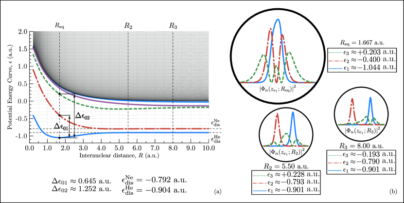
Figure 2: (a) Potential Energy Curves (PECs) of the one-dimensional $\text{NeHe}^{+}$ ion as a function of internuclear distance within the Born-Oppenheimer approximation. The first 500 eigenenergies are shown, with a grayscale gradient representing the continuum of energy levels. The horizontal dashed lines indicate the ionization energies of the Helium atom ($\epsilon_{\text{dis}}^{\text{He}}$) and of the Neon atom ($\epsilon_{\text{dis}}^{\text{Ne}}$) respectively. Furthermore, $\Delta\epsilon_{01}$ and $\Delta\epsilon_{02}$ are the energy differences at equilibrium distance between the ground state energy and the first and second excited state energies, respectively. (b) Electronic densities for the first three energy levels, obtained by solving the Time-Independent Schrödinger Equation (TISE) at selected internuclear distances. All calculations were performed using the FEMTISE package [32].

IV.1 PECs for $\text{NeHe}^{+}$

The PECs for the $\text{NeHe}^{+}$ ion are computed by solving Eq. (14) for different values of $R$ and are shown in Fig. 2(a). Only the ground and first 2 excited states can bind vibrational nuclear states. Above the fifth curve, an accumulation of curves is developed that signals the pseudo-continuum onset (grayscale gradient). The dissociation limits ($R\rightarrow\infty$) of the ground (first excited) curve corresponds to the Helium (Neon) first ionization energy, and the corresponding electronic density is shown in Fig. 2(b) for $R=8.0\text{ a.u.}$. The states show that according to our setup in Fig. 1, the Helium is on the right and the Neon is on the left. The equilibrium distance for the ground state $R_{\text{eq}}\approx 1.67\text{ a.u.}$ is below the experimental values reported for the molecule [30]. The Yukawa interactions proposed here aim to model a one-dimensional system with tunable interactions and to show the effect of electron-nuclear dynamics on quantum correlations (and ICEC) and, within its limitations, the model correctly reproduces some characteristic of the $NeHe^{+}$ ion, but could not reproduce the $R_{eq}$ more accurately.

The density corresponding to the second excited state near the equilibrium distance of this state is shown in Fig. 2(b) for $R_{2}=5.50\text{ a.u.}$. It shows how the electronic density is increased between the nuclei and provides binding. For longer distances, $R_{3}=8.00\text{ a.u.}$, this state develops into an excited state for the Helium atom as is apparent from the inset.

The energy differences $\Delta\epsilon_{01}$ and $\Delta\epsilon_{02}$, between the ground state energy at $R_{\text{eq}}$ and the first and second excited state energies, are useful to determine the energy at which one expects the ICEC channel to be open. This is true in a fixed nuclei approach, however this activation energies are modified by the inclusion of nuclei dynamics as shown in Ref. [7]. Moreover, new paths that can be quite different appear by inclusion of the nuclei dynamics and will be described in the next section.

IV.2 Scattering details

This sections depicts how to study the time dependent electronic and nuclear densities and how to spot different characteristics and scattering channels from the time evolution. The dynamics published in Ref. [7], using different interaction potentials, where focused on the main differences between fixed nuclei and full dynamics. The abbreviated analysis presented here is useful in the following sections where it is contrasted to the one performed using the information obtained from the von Neumann and Shannon entropies.

The dynamics of the electronic scattering against $\text{NeHe}^{+}$ depends, mostly, on the energy distribution of the incoming wave packet. The effect of three different incoming energies is discussed: below the first excited state ($\varepsilon_{\text{in}}=0.4\,\mbox{a.u}<\Delta\epsilon_{01}$), above the first excited state ($\Delta\epsilon_{02}>\varepsilon_{\text{in}}=0.4\,\mbox{a.u.}>\Delta\epsilon_{01}$) and near the second excited state vertical threshold ($\varepsilon_{\text{in}}=1.2\,\mbox{a.u.}\approx\Delta\epsilon_{02}$). The energy dispersion of the projectile wave packet ($\Delta\varepsilon=0.06\,\mbox{a.u.}$) is the same in the three cases. The time-dependent electronic and nuclear densities are shown in Fig. 3.

For the lower energy, the electronic density, Fig. 3(a), shows an incoming Gaussian shaped density from the left and impacting the $\text{NeHe}^{+}$ molecule (at the indicated impact time) and resulting in a reflected and transmitted densities. Both of these densities show no large changes in energy, which can be identified from the slope of the peak values of the densities. Only the characteristic spreading of the Gaussian wave packet in both cases is observed. Hence, only an elastic scattering channel seems to be open. However, the nuclear densities (Fig. 3(d)) give a deeper insight and make apparent a vibrational excitation of the nuclei and, moreover, a dissociation channel of the nuclei. The vibrational excitation shows that there is an inelastic vibrational channel, restricted to the ground state $\epsilon_{0}(R)$. The absorption of density by the CAPs at the grid edge makes apparent that the emitted electronic density is in the same channel to most of the vibrational excitations, since the nuclei density is strongly reduced at the same time that the electronic density is absorbed at the grid edge (around $15\mbox{ fs}$). There is, however, density that survives this absorption: A small vibrational density localized near the equilibrium distance and two dissociation branches (the two lines with similar slopes). The electronic density that is connected to this two contributions is shown by the inset in Fig. 3(a). The densities show that some density is bound to the molecule and the rest is evolving with the dissociation channel.

The setup with energy $\varepsilon_{\text{in}}=0.8\,\mbox{a.u.}$ (see Figs. 3(b) and 3(e)) includes clear evidence of inelastic electronic emission. The process is detected by noting that after the collision we observe two different peaks for the electronic density with different slopes. One has the same energy as the incoming wave packet while the other is a slower electron emission with a slope compatible to the ICEC process to the first excited state. The nuclear density shows two main channels: an elastic density, that stays localized near $R_{\text{eq}}$, which is absorbed when the elastic electron reaches the grid edge (around $10$ fs) and a dissociation channel, that is absorbed by the time the ICEC electron reaches the grid edge (around $15$ fs ). This is the clear indication that the dissociation is mainly due to ICEC. Specifically, the incoming electron is captured by the molecule in the dissociative first excited state and the excess energy is taken by the bound electron which is, in this case, emitted with a lower energy than the incoming one. The capture in the first excited state is made evident by the inset of Fig. 3(b), noting that the structure is that of the electronic state densities depicted in Fig. 2(b) at $R_{\text{eq}}$.

The higher energy case, $\varepsilon_{\text{in}}=1.2\,\text{a.u.}$ (see Figs. 3(b) and 3(e)), involves three different density branches: the elastic channel (EC) with the smaller slope, the first excited state ICEC channel (ICEC₁) with a middle slope and the second excited ICEC channel (ICEC₂) with the higher slope. The EC and ICEC₁ channels are the most intense ones, and hence the two most probable processes to happen. The ICEC₂ is much more less intense, and hence less probable. EC and ICEC₁ have a higher probability in the forward direction than in the backward direction which contrasts with the rather equally probable forward and backward emission of ICEC₂. One important difference between ICEC₁ and ICEC₂ is the symmetry of the electronic density (see Fig. 2(b)) which is asymmetric in channel 1 ($|\xi_{2}|^{2}$) and nearly symmetric in channel 2 ($|\xi_{3}|^{2}$). Moreover, the incident electron comes from the left and the capture into ICEC₁ eases the emission to the right of the bound electron. On the other hand, for ICEC₂ the effect is compensated by the fact that the second excited state density at $R_{eq}$ is surrounding the density for the ground state, giving an equally probable forward and backward emission.

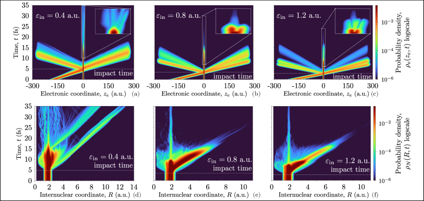
Figure 3: Electronic and nuclear probability densities at various incoming electron energies. The insets illustrate magnified views of the electronic probability density over specified spatial and temporal ranges: (a) electronic coordinate range from $-12$ to $12$ a.u. and evolution time from $10$ to $35$ fs, (b) electronic coordinate range from $-8$ to $8$ a.u. and evolution time from $7$ to $30$ fs, (c) electronic coordinate range from $-11$ to $11$ a.u. and evolution time from $6$ to $24$ fs. The horizontal dashed line marks the collision zone.

IV.3 Dynamics of quantum information measures

The entanglement and correlations between the different bipartions of a physical system can be quantified using the von Neumann and Shannon entropies, as well as mutual information, as defined in Sections III.5.1, III.5.2 and III.5.3. Here we describe how entanglement and mutual information evolves in time during the collision process.

IV.3.1 Von Neumann entropy

The results for the case of low incoming electron energy ($\varepsilon_{\text{in}}=0.4\,\text{a.u.}$) are discussed first. Figure 4 shows the von Neumann entropies for the target-projectile entanglement $S^{\text{vN}}_{e}$ and for the nuclei-electrons entanglement $S^{\text{vN}}_{N}$, along with the norm, electronic dispersion and electronic position.

The electronic dispersion $\Delta\hat{z}_{e}$, is rather large at the initial time up to values very close to the "collision time" were it shows a minimum. This is because the electronic state is properly antisymmetrized, hence the probability density is double peaked, and the dispersion reflects this two peaked distribution. The minimum at the collision is not only due this two peaked distribution coming together, but also to a squeezing of the incoming wave packet due to the strong repulsive interaction with the bound electron. As presented here, the "collision time" is a rather loose concept, since it depends, as we will see on Sec. IV.4, on the quantity one uses to define it.

Noticeable, the target-projectile entanglement entropy ($S^{\text{vN}}_{e}$) develops a peak near this collision time . More interesting is that, previous to the collision, $S^{\text{vN}}_{e}$ has a value corresponding to a maximally mixed electronic reduced density (because it includes the entanglement between the bound and incoming electron), and after peaking at the collision time ($\approx 5\text{ fs}$) it stabilizes again to a higher value than the initial one (this may not by the case in two particle scattering, see Ref. [44]). In other words, the initial entanglement measure is highly increased in the collision, but not all of it is retained. Thus a natural question raises is how much of this entanglement is retained in different scenarios. We will discuss this in Sec. IV.5.

The collision effect is also visible in the nuclei-electron entanglement entropy, since it raises from a nearly zero value up to a plateau. However, there is no peak in the entanglement during the collision. The entanglement increase clearly shows that during the collision the nuclei and electrons strongly correlate and that this entanglement is sustained in time.

The natural orbital populations $\lambda^{(\alpha)}_{j}$ (used to compute the von Neumann entropies, as shown in Eq. (28)) indicate that many electronic populations climb up to rather high values at the collision, and then decrease. This points to vibrations being temporarily excited during the collision. Also one can connect the wave packet squeezing at collision time to this raise and decrease of the populations. This is shown in the Appendix C.

After all collision effects are over, the emitted electron is absorbed by CAP at the grid edge. This absorption leads to a loose in norm, as seen in Fig. 4 from $10\text{ fs}$ on. This has an important effect on the entropies and mean values, since the absorbed probability density of the particle (and its corresponding terms in the wave function expansion) are no longer part of the system, and one must be careful in the interpretation of the results.

The changes in the entropies, due to the absorption can be used to detect the different channels present for a given energy. Figs. 4, 5 and 6 show the time dependent entropies for the three cases shown in Fig. 3. For $\varepsilon_{\text{in}}=0.4\text{ a.u.}$, since the absorption is rather smooth and all of the entropy goes to zero, only the elastic channel is present.

In the case of $\varepsilon_{\text{in}}=0.8\text{ a.u.}$, one can see that the absorption starts at $8\text{ fs}$, an then has a small plateau at $10\text{ fs}$, after which it decays again until it vanishes. This behavior matches exactly the absorption of the two present channels: the elastic and ICEC to the first excited state. The decay between 8 and 10 fs corresponds to the absorption of the elastic channel, after which, a small period of time with no absorption follows. This small plateau, which lives until the slower ICEC electron reaches the CAP, gives the entropy contribution of ICEC. The entropy decays again after the plateau, at a different pace than in the elastic channel. This analysis shows that combining entropy and CAPs in this setup allows to detect the different channels. This is even more apparent for $\varepsilon_{\text{in}}=1.2\text{a.u.}$, where the system have elastic, ICEC₁ and ICEC₂ emitted electrons. The three absorptions can be identified in the entropies, and clear differences in absorption time and the plateaus are seen for the channels.

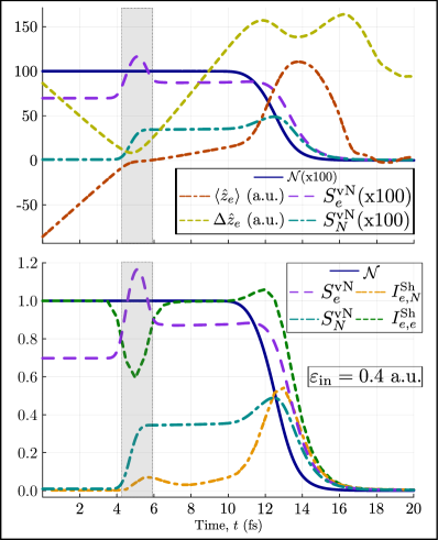
Figure 4: For an incoming electron energy of $0.4\text{ a.u.}$, the top panel shows the expectation value of the electron position ($\left\langle\hat{z}_{e}\right\rangle$), the electronic position dispersion ($\Delta\hat{z}_{e}$), the target-projectile entanglement entropy ($S_{e}^{\text{vN}}$), the nuclei-electron entanglement entropy ($S_{N}^{\text{vN}}$) and the norm ($\mathcal{N}$). The bottom panel displays $S_{e}^{\text{vN}}$, $S_{N}^{\text{vN}}$, the electron-electron Shannon mutual information ($I_{e,e}^{\text{Sh}}$,), the target-projectile Shannon mutual information ($I_{e,N}^{\text{Sh}}$,) and the norm. The shaded region indicates where the collision occurs.

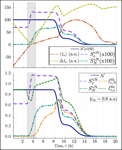
Figure 5: Same as in Fig. 4, for an incoming electron energy of $0.8\text{ a.u.}$.

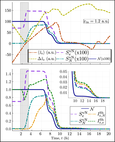
Figure 6: Same as in Fig. 4, for an incoming electron energy of $1.2\text{ a.u.}$. Additionally, the inset provides an amplified view of the quantities for evolution times greater than $8\,\text{fs}$, where only $\text{ICEC}_{2}$ channel is left, this made apparent by a plateau in the plotted curve.

IV.3.2 Mutual informations

The mutual information defined in Section III.5.3, can be computed for the electron-electron or the electron-nuclei pair. Fig. 7 shows the behavior of the Shannon mutual information as compared to the conditional von Neumann mutual information.

At the time of the collision, the electron-electron Shannon mutual information ($I_{e,e}^{\text{Sh}}$) (see Fig. 7(c)) reaches a local minimum, indicating a reduction in classical correlations between the electrons. This implies that less classical information about one electron can be inferred by measuring the other. In contrast, during the collision, both the target-projectile von Neumann entropy ($S_{e}^{\text{vN}}$) (see Figs. 4, 5 and 6) and the electron-electron conditional von Neumann mutual information ($I_{e,e}^{\text{vN}}$) (see Fig. 7(a)) show local maxima. The increase in $S_{e}^{\text{vN}}$ reflects an enhancement in target-projectile entanglement, as discussed in Sec. III.5.3. Similarly, the rise in $I_{e,e}^{\text{vN}}$ suggests that all quantum correlations, including enhanced correlations and non-locality between electrons, intensify. Another noticeable difference between these quantities is that they refer to correlations in different subsystems. The entropy $S_{e}^{\text{vN}}$ describes entanglement between the target and projectile, while $I_{e,e}^{\text{vN}}$ refers to the quantum correlations between electrons, conditioned on the measurement of the nucleus. For the low energy case there are no new correlations between electrons, as the value is the same before and after the collision ($I^{\text{vN}}_{e,e}$). There is entanglement between electrons and nuclei, since the nuclei are vibrationally excited in this case ($I^{\text{vN}}_{e,e}\equiv S^{\text{vN}}_{N}$). For higher energies, correlations between electrons are build up due to the inelastic excitation of the bound electron, and also nuclei-electron correlations grow even more as they include vibrations and excitations.

After the collision time, when a certain percentage of the elastic channel density is absorbed by the CAP, both the electron-nuclei Shannon mutual information ($I_{e,N}^{\text{Sh}}$) and the electron-nuclei conditional von Neumann mutual information ($I_{e,N}^{\text{vN}}$) exhibit global maxima. This is because the density absorbed at the CAP corresponds to the elastic channel, which does not contribute to the mutual information (the mutual information is zero before collision). Hence, the mutual information of the remaining density is higher because it does not have the uncorrelated density contributions (the norm is decreasing, see Figs. 4, 5 and 6). The collision enhances electron-nucleus correlation, encompassing both classical and quantum components. In addition, it is observed that $I_{e,N}^{\text{vN}}$, for high incoming electron energies, exhibits peaks that are greater than or equal in magnitude to those of $I_{e,N}^{\text{Sh}}$. This occurs because the von Neumann mutual information captures not only classical correlations but also quantum correlations. At higher energies, more ICEC channels become available, which involve additional quantum correlations. This information is detectable only through the von Neumann mutual information, as the Shannon mutual information accounts solely for classical correlations.

The nuclei-electron entanglement entropy ($S_{N}^{\text{vN}}$), turns out to be equivalent to $I_{e,N}^{\text{vN}}$ in the present case (see Eq. (40)). Since $I_{e,N}^{\text{vN}}$ reflects the quantum correlations between an electron and the nuclei, they are thus all due to entanglement between them. Also, the knowledge of one electron state is not a significant factor in quantifying nuclei-electrons entanglement, because they are identical particles.

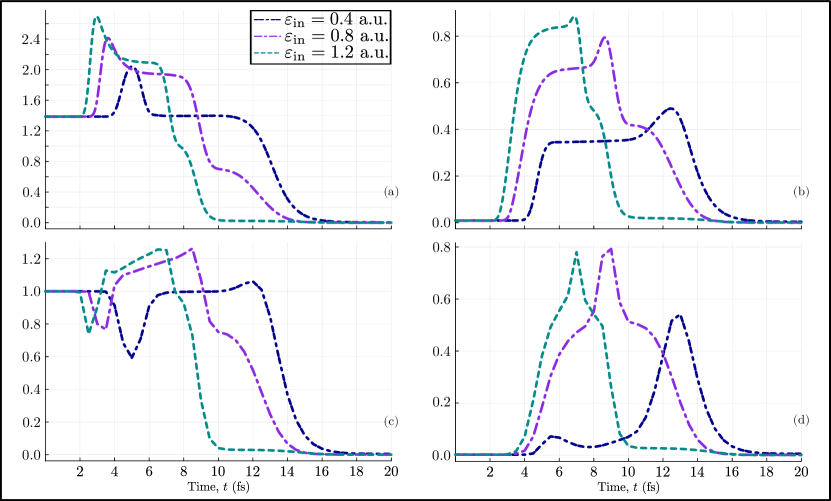
Figure 7: Time evolution of mutual informations for different electron incoming energies: (a) electron-electron conditional von Neumann mutual information, $I_{e,e}^{\text{vN}}$, (b) electron-nuclei conditional von Neumann mutual information, $I_{e,N}^{\text{vN}}$, (c) electron-electron Shannon mutual information, $I_{e,e}^{\text{Sh}}$, and (d) electron-nuclei Shannon mutual information, $I_{e,N}^{\text{Sh}}$.

IV.4 Impact time estimation and information measures

The collision event can be spotted using different quantities. For example, the von Neumann electronic entropy ($S^{\text{vN}}_{e}$) and the electron-electron conditional von Neumann mutual information ($I^{\text{vN}}_{e,N}$) both show maximum values within the collision region, while electronic dispersion ($\Delta\hat{z}_{e}$) and electro-electron Shannon mutual information show minimum values $I_{e,e}^{\text{vN}}$. There is need to properly define a collision time ($t_{\text{col}}$) in order to compare the entanglement at that particular time with the entanglement before ($t_{\text{be}}=t_{\text{col}}-\Delta t$) and after ($t_{\text{af}}=t_{\text{col}}+\Delta t$) the collision. The collision time can be estimated analyzing those quantum information measures in the collision region ($\mathcal{I}_{\text{col}}=[t_{\text{be}},t_{\text{af}}]$), that is,

$$t_{\text{col}}^{S}\text{ }: S_{e}^{\text{vN}}\left(t_{\text{col}}^{S}\right)\geq S_{e}^{\text{vN}}(t) \forall t\in\mathcal{I}_{\text{col}},$$ (43)

$$t_{\text{col}}^{\Delta}\text{ }: \Delta\hat{z}_{e_{i}}\left(t_{\text{col}}^{\Delta}\right)\leq\Delta\hat{z}_{e_{i}}(t) \forall t\in\mathcal{I}_{\text{col}},$$ (44)

$$t_{\text{col}}^{I}\text{ }: I_{e,e}^{\text{Sh}}\left(t_{\text{col}}^{I}\right)\leq I_{e,e}^{\text{Sh}}(t) \forall t\in\mathcal{I}_{\text{col}}.$$ (45)

The results are presented in Figure 8. For low energies, below $0.2$ a.u., the collision time estimation by electronic dispersion is significantly higher than the time estimations by electronic Shannon mutual information or by von Neumann electronic entropy. This result is due to the electron incoming energy is not enough to produce a significant transmitted electronic density, therefore the majority of electronic density is reflected and, at the collision region, there is a high electronic dispersion, the collision is not clearly seen, and hence the estimation by electronic dispersion is not accurate.

At intermediate energies, from $0.2$ a.u. to $0.8$ a.u., all the estimated collision times are similar.

Finally, at high energies, above $0.8$ a.u., the estimation of collision time by the von Neumann electronic entropy is slightly higher than the other time estimations. The essence of this different estimation is that the electronic Shannon mutual information and the electronic dispersion are measuring classical correlations of the electronic system. On the other hand, the estimation time by von Neumann electronic entropy takes into account the entanglement between electronic and nuclear subsystem.

The von Neumann electronic entropy is then best suitable as an estimator to give a proper "collision time" in this type of quantum collision dynamics using wave packets, since it includes quantum entanglement which is one of the characteristic features of the collision.

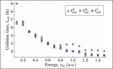
Figure 8: Estimated impact time as a function of incoming electron energies, determined by extreme values of electronic von Neumann entropy ($t_{\text{col}}^{S}$), electron-electron mutual information ($t_{\text{col}}^{I}$) and electronic dispersion ($t_{\text{col}}^{\Delta}$).

IV.5 Entanglement generation

Once the collision time was estimated as described in IV.4, one is able to compute how much relative electron-nucleus entanglement is present as,

$$\delta_{S}(t)=\frac{S_{e}^{\text{vN}}(t)}{S_{e}^{\text{vN}}(t_{\text{col}})}.$$ (46)

It is also interesting to compare the entanglement before the collision with that at the collision time $t_{col}$, since during the collision the quantum correlations are highly increased.

There is an energy range (see Figure 9), from $0.2$ a.u. to $0.7$ a.u., where from the total electron-nuclei entanglement generated at the collision time, about $20\%$ is lost after the collision. At higher energies, most of the entanglement is conserved after the collision. The reason is that there is many available channels at higher energies, and correlations to this states can be created easily and thus keeping it in the system. For lower energies, the number of accessible channels is more reduced, the transition matrix elements may also be small, and thus a part of the entanglement generated is lost because the system goes back to lower energy levels.

The relative value of entropy before the collision gives a hint on how much entanglement is generated. It also shows a region, from $0.5$ a.u. to $0.7$ a.u., where the generated entanglement is reduced from the trend. For $\varepsilon_{\text{in}}=0.5$ a.u., from the total amount of generated entanglement, about $60\%$ is initial entanglement, while for $\varepsilon_{\text{in}}=0.6$ a.u. this rises to $70\%$a.u. The reason is that the energies are approaching the first excited state energy threshold $\Delta\epsilon_{01}$. A similar effect is seen for energies from $1.0$ a.u. to $1.2$ a.u., again matching to the onset of the second excited state threshold $\Delta\epsilon_{02}$. The result is that near the threshold values, a less amount of entanglement can be generated at the collision.

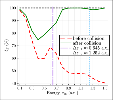
Figure 9: The relative von Neumann entropies ($\delta_{S}$) as a function of incoming electron energies. The plot shows the relative entropy values evaluated at times before ($t_{be}$) and after ($t_{af}$) the collision. Vertical dashed lines represent the energy differences at equilibrium distance between the ground state energy and the first excited state ($\Delta\epsilon_{01}$) and second excited state ($\Delta\epsilon_{02}$).

V CONCLUSION

The work analyze entanglement and correlations measures of an inelastic electron capture and emission process (ICEC) by a dimer molecule, in which the nuclei movement is fully included. Long-range interactions (Coulomb potential) for electron-electron repulsion and a short-range interactions (Yukawa potential) for electron-nucleus attraction and nucleus-nucleus repulsion are used. The Yukawa potential simulates electron screening effects, and the electrons were treated as identical particles. Moreover, based on previous works [13], an effective one-dimensional potential is constructed to account for harmonic confinement. This confinement can also be used to model realistic boundary conditions in trapped ion systems or quantum dots, and it is also relevant for exploring phenomena such as quantum phase transitions and collective excitations in confined systems.

The results from the probability densities give an understanding about collision time and zone, elastic and inelastic scattering, the symmetry of the electronic states and dissociation mechanisms. A novel approach to analyze the collision dynamics using quantum information theory measures, such as von Neumann’s entropy and conditional mutual information was introduced. The comparison with previously used quantities such as the Shannon entropy is also presented  [11, 45]. These quantities enable the identification of the number and type of scattering channels (elastic and inelastic) during propagation, as well as the quantification of quantum and classical correlations between subsystems. Additionally, the collision time is estimated using three specific quantum information metrics. The amount of entanglement preserved after the collision and the entanglement generated by the scattering process is discussed and seen to be highly connected to inelastic processes. The energy range were the inelastic processes are active show that most of the entanglement is kept after collision. Besides the main topics studied, a self-developed software package [32] (implemented in Julia) to compute potential energy curves (PECs) was developed.

As a future line of work, it would be of interest to implement a quantum discord measure [46] for these systems, since it is seen here that correlations and entanglement differ in the collision process. Another interesting point about the ICEC process is the actual time it takes the process to happen, since this would be an important tool to estimate whether ICEC can be measured in an experiment or not. An analysis of this particular point could be done using the present dynamical description, by setting up different initial conditions corresponding to experimental setups.

VI Author contributions

M.M. designed and developed the FEMTISE software and run all the calculations on MCTDH. M.M. and F.M.P. equally contributed to scientific conceptualization, formal analysis and manuscript writing.

Appendix A Building the initial state in MCTDH-Heidelberg package

The initial state for the quantum evolution is the properley symmetrized product state of the ground state of $\text{NeHe}^{+}$ ion model with one active electron times a gaussian for the projectile electron. The Hamiltonian for the ground state is given by,

$$\hat{H}_{e_{1},R}=\hat{T}_{e_{1}}+\hat{T}_{N}+\hat{V}^{(e_{1}c_{\text{He}})}_{\text{eff}}+\hat{V}^{(e_{1}c_{\text{Ne}})}_{\text{eff}}+\hat{V}^{(c_{\text{Ne}}c_{\text{He}})}_{\text{eff}}$$ (47)

Table 3: Setting for $\text{NeHe}^{+}$ ion relaxation using MCTDH-Heidelberg package.

Symbol	Description	Value [au]
$N_{z_{e}}$	number of points for DVR grid	1501
$N_{R}$	number of points for DVR grid	501
$(z_{e}^{\text{min}},z_{e}^{\text{max}})$	electronic grid domain range	(-300, 300)
$(R^{\text{min}},R^{\text{max}})$	nuclear grid domain range	(0, 20)
$\text{SPF}_{z{e}}$	number of electronic SPFs	20
$\text{SPF}_{R}$	number of nuclear SPFs	18
$\text{tol}_{\text{CMF}}$	tolerance of CMF integrator	$10^{-3}$
$\text{tol}_{\text{RK8/spf}}$	tolerance of RK8 integrator	$10^{-9}$
$\text{tol}_{\text{rrDAV/A}}$	tolerance of rrDAV integrator	$10^{-8}$
$\text{tol}_{\text{eps inv}}$	tolerance of eps inv integrator	$10^{-10}$
$t_{\text{final}}$	final relaxation time	$82.6841$
$t_{\text{out}}$	step relaxation time	$0.4134$

The relaxation to the ground state of the Hamiltonian (47) is performed using imaginary time propagation as implemented in the MCTDH Heildeberg package [39]. This relaxation is performed from specific ansatz for each DOF: for $z_{e_{1}}$ corresponds to the ground state of the Hamiltonian in Eq. (15), except here the internuclear coordinate is fixed at the equilibrium value of the ground-state PEC $(R_{\text{eq}})$, for $R$ corresponds to the ground state of the Hamiltonian given by $\hat{H}_{R}=\hat{T}_{R}+\epsilon_{0}(R)$, where $\epsilon_{0}(R)$ refers to the PEC of the ground state (see Fig. 2(a)). The simulations were performed using the configurations shown in Table 3.

Once the ground state of the Hamiltonian (47) is obtained, the product with the Gaussian of the incoming electron must be included. Actually, due to the algorithm implementation, the electron incoming electron DOF, say $z_{e_{2}}$, is already included as a product to a Gaussian with no interaction to $R$ or $z_{e_{1}}$.

In general terms, in the MCTDH-algorithm, the wave function is written as a Hartree product [39],

$$\Psi(q_{1},q_{2},\dotsc,q_{n},t)=\sum_{j_{1}=1}^{n_{1}}\dotsc\sum_{j_{f}=1}^{n_{f}}A_{j_{1}\dotsc j_{f}}(t)\times$$

$$\times\prod_{k=1}^{f}\varphi_{j_{k}}^{(k)}(q_{k},t)$$ (48)

where $\left\{\varphi_{j_{k}}^{(k)}(q_{k},t)\right\}_{j_{k}=1}^{n_{k}}$ represents the single particle function (SPF) time-dependent basis for the degree of freedom (DOF) $q_{k}$, and $A_{j_{1}\dotsc j_{f}}(t)$ are the time-dependent coefficients that control the phase selection of each (SPF).

In our case, we obtained the relaxation of the $\text{NeHe}^{+}$ ion, thus the initial wave functions at this stage of the simulation are given by:

$$\Psi_{\text{relax}}^{\text{ini}} = \sum_{j_{1},j_{2},j_{3}}A_{j_{1}j_{2}j_{3}}^{\text{relax}}\phi_{j_{1}}^{(e_{1})}(z_{e_{1}})\phi_{j_{2}}^{(N)}(R)\phi_{j_{3}}^{(e_{2})}(z_{e_{2}})$$ (49)

$$= \sum_{j=1}^{n}A_{jj1}^{\text{relax}}\phi_{j}^{(e_{1})}(z_{e_{1}})\phi_{j}^{(N)}(R)$$

were we consider only a single trivial term in the projectile’s SPF basis (with $n_{3}=1$ and $\phi_{1}^{(e_{2})}(z_{e_{2}})=1$). The $A_{jj1}^{\text{relax}}$ coefficients are the only non-zero coefficients obtained from the relaxation, and we note that only the diagonal terms ($j_{1}=j_{2}=j$) persist.

After relaxation step, we define a Gaussian wave packet for the projectile, while maintaining the same Hartree product configuration for the target,

$$\Psi_{\text{punch}}^{\text{ini}}=\sum_{j}A_{jj1}^{\text{relax}}\phi_{j}^{(e_{1})}(z_{e_{1}})\phi_{j}^{(N)}(R)\phi_{1}^{\left(\text{gauss}\right)}(z_{e_{2}}).$$ (50)

We then need to build a symmetric state for the electronic coordinates and, by setting symorb=1,3 MCTDH keyword, a global SPF basis is constructed for the electronic system from the individual SPF basis associated to each electron as follows,

$$\begin{pmatrix}\left\{\varphi_{j_{1}}^{(e_{1})}(z_{e_{1}})\right\}_{j_{1}=1}^{n_{1}}&\left\{\varphi_{j_{2}}^{(e_{2})}(z_{e_{2}})\right\}_{j_{2}=1}^{n_{2}}&\left\{\varphi_{j}^{(e)}(z_{e})\right\}_{j=1}^{n}\\ \phi_{1}^{(e_{1})}(z_{e_{1}})&\phi_{1}^{(e_{2})}(z_{e_{2}})&\phi_{1}^{(e)}(z_{e})=\phi_{1}^{(e_{1})}\\ \phi_{2}^{(e_{1})}(z_{e_{1}})&\phi_{2}^{(e_{2})}(z_{e_{2}})&\phi_{2}^{(e)}(z_{e})=\phi_{1}^{(e_{2})}\\ \phi_{3}^{(e_{1})}(z_{e_{1}})&\phi_{3}^{(e_{2})}(z_{e_{2}})&\phi_{3}^{(e)}(z_{e})=\phi_{2}^{(e_{1})}\\ \phi_{4}^{(e_{1})}(z_{e_{1}})&\phi_{4}^{(e_{2})}(z_{e_{2}})&\phi_{4}^{(e)}(z_{e})=\phi_{2}^{(e_{2})}\\ \phi_{5}^{(e_{1})}(z_{e_{1}})&\phi_{5}^{(e_{2})}(z_{e_{2}})&\phi_{5}^{(e)}(z_{e})=\phi_{3}^{(e_{1})}\\ \phi_{6}^{(e_{1})}(z_{e_{1}})&\phi_{6}^{(e_{2})}(z_{e_{2}})&\phi_{6}^{(e)}(z_{e})=\phi_{3}^{(e_{2})}\\ \phi_{7}^{(e_{1})}(z_{e_{1}})&\phi_{7}^{(e_{2})}(z_{e_{2}})&\phi_{7}^{(e)}(z_{e})=\phi_{4}^{(e_{1})}\\ \phi_{8}^{(e_{1})}(z_{e_{1}})&\phi_{8}^{(e_{2})}(z_{e_{2}})&\phi_{8}^{(e)}(z_{e})=\phi_{4}^{(e_{2})}\\ \phi_{9}^{(e_{1})}(z_{e_{1}})&\phi_{9}^{(e_{2})}(z_{e_{2}})&\phi_{9}^{(e)}(z_{e})=\phi_{5}^{(e_{1})}\\ \vdots&\vdots&\vdots\end{pmatrix},$$ (51)

and using the symmetrization operator ($\hat{\mathcal{S}}$), we can express the initial wave functions of the $\text{NeHe}^{+}$ ion as an expansion in terms of the previously defined electronic basis as follows:

$$\Psi_{\text{symm}}^{\text{init}}=\sum_{j=1}^{n}A_{jj1}^{\text{relax}}\hat{\mathcal{S}}\left\{\phi_{(2j-1)}^{(e)}(z_{e_{1}})\phi_{2}^{(e)}(z_{e_{2}})\right\}\phi_{j}^{(N)},$$ (52)

The symmetrized state is then expressed according to the general expansion in Eq. (A),

$$\Psi_{\text{symm}}^{\text{init}}=\sum_{j_{1},j_{2},j_{3}}A_{j_{1}j_{2}j_{3}}^{\text{symm}}\phi_{j_{1}}^{(e_{1})}(z_{e_{1}})\phi_{j_{2}}^{(N)}(R)\phi_{j_{3}}^{(e_{2})}(z_{e_{2}})$$ (53)

where the coefficients $A_{j_{1}j_{2}j_{3}}^{\text{symm}}$ must satisfy the condition that: if $j_{1}=(2j_{2}-1)$, $j_{2}=j$ with $j\in\mathbb{N}$ and $j_{3}=2$ then:

$$A_{(2j-1)j2}^{\text{symm}}=A_{2j(2j-1)}^{\text{symm}}=A_{jj1}^{\text{relax}}$$ (54)

Once the coefficient $j$ is fixed, the value of $A_{j_{1}j_{2}j_{3}}^{\text{symm}}$ is likewise determined.

Appendix B Propagation setups for MCTDH-Heidelberg package

The full three-dimensional system is propagated with the MCTDH algorithm as implemented in Ref. [39]. There are three DOFs $z_{e_{1}}$, $R$ and $z_{e_{2}}$, and we treating the electrons as identical particles (using the same SPFs) in a symmetrical electronic state. The initial state is defined according to the results from the relaxation stage (see Appendix A). The simulations were performed using the parameters listed in Table 4.

Table 4: Setting for the propagation of electron-ion scattering using MCTDH-Heidelberg package.

Symbol	Description	Value [au]
$N_{z_{e}}$	number of points for DVR grid	1501
$N_{R}$	number of points for DVR grid	501
$(z_{e}^{\text{min}},z_{e}^{\text{max}})$	electronic grid domain range	(-300, 300)
$(R^{\text{min}},R^{\text{max}})$	nuclear grid domain range	(0, 20)
$\text{SPF}_{z_{e}}$	number of electronic SPFs	20
$\text{SPF}_{R}$	number of nuclear SPFs	18
$\text{tol}_{\text{CMF/var}}$	tolerance of CMF integrator	$10^{-7}$
$\text{tol}_{\text{BS/spf}}$	tolerance of BS integrator	$10^{-8}$
$\text{tol}_{\text{SIL/A}}$	tolerance of SIL integrator	$10^{-7}$
$t_{\text{final}}$	final relaxation time	$1446.9481$
$t_{\text{out}}$	step relaxation time	$0.4134$

Appendix C Natural orbital population

Initially, only a few natural orbitals have significant populations, indicating that the initial state of the system is well-described, as we can see in Fig. 10. We also observe that, for the electronic state, two orbitals are more populated than the others, while for the nuclear state, only one orbital has a higher population than the rest. At the moment of collision, the most populated electronic and nuclear orbitals slightly decrease in population, whereas the less populated orbitals significantly increase in population. This indicates that, at the moment of collision, representing the system’s state becomes more challenging, requiring more coefficients for an accurate description, as seen in Eq. (27).

After the collision, the natural orbitals that increased in population during the collision begin to decrease, making it easier to represent the state. However, as energy increases, this decrease in orbital population becomes less pronounced. This is because, at higher energies, more ICEC channels are involved, and the inelastic scattering process generates significant correlations in the system, requiring more coefficients to represent the state than in the low-energy case, where only elastic scattering occurs. Finally, at long times, the populations decrease significantly due to the presence of complex absorbing potentials (CAPs), which absorb electronic and nuclear density, causing the orbital norm not to be conserved over time.

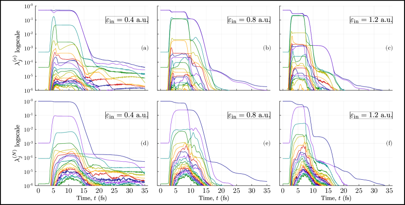
Figure 10: Time evolution of natural orbital populations. The top panels show the electronic natural orbital populations ($\lambda^{(e)}_{j}$) and the bottom panels show the nuclear natural orbital populations ($\lambda^{(N)}_{j}$). The panels (a) and (d) correspond to an incoming electron energy of $0.4\text{ a.u.}$, the panels (b) and (e) correspond to an incoming electron energy of $0.8\text{ a.u.}$ and the panels (c) and (f) correspond to an incoming electron energy of $1.2\text{ a.u.}$.

References

- Sisourat et al. [2010] N. Sisourat, H. Sann, N. V. Kryzhevoi, P. Kolorenč, T. Havermeier, F. Sturm, T. Jahnke, H.-K. Kim, R. Dörner, and L. S. Cederbaum, Interatomic Electronic Decay Driven by Nuclear Motion, Phys. Rev. Lett. 105, 173401 (2010), publisher: American Physical Society.
- Otto et al. [2008] F. Otto, F. Gatti, and H.-D. Meyer, Rotational excitations in para-H[sub 2]+para-H[sub 2] collisions: Full- and reduced-dimensional quantum wave packet studies comparing different potential energy surfaces, The Journal of Chemical Physics 128, 064305 (2008).
- Arnold et al. [2018] C. Arnold, O. Vendrell, R. Welsch, and R. Santra, Control of Nuclear Dynamics through Conical Intersections and Electronic Coherences, Phys. Rev. Lett. 120, 123001 (2018).
- Haxton et al. [2011] D. J. Haxton, K. V. Lawler, and C. W. McCurdy, Multiconfiguration time-dependent Hartree-Fock treatment of electronic and nuclear dynamics in diatomic molecules, Phys. Rev. A 83, 063416 (2011), publisher: American Physical Society.
- Albrecht et al. [2023] P. A. Albrecht, C. Witzorky, P. Saalfrank, and T. Klamroth, Approximation Schemes to Include Nuclear Motion in Laser-Driven Ab Initio Electron Dynamics: Application to High Harmonic Generation, J. Phys. Chem. A 127, 5942 (2023), publisher: American Chemical Society.
- Palacios et al. [2015] A. Palacios, J. L. Sanz-Vicario, and F. Martín, Theoretical methods for attosecond electron and nuclear dynamics: applications to the H molecule, Journal of Physics B: Atomic, Molecular and Optical Physics 48, 242001 (2015).
- Pont et al. [2024] F. M. Pont, A. Bande, E. Fasshauer, A. Molle, D. Peláez, and N. Sisourat, Impact of the nuclear motion on the interparticle Coulombic electron capture, Phys. Rev. A 110, 042804 (2024).
- Dey et al. [2022] D. Dey, A. I. Kuleff, and G. A. Worth, Quantum Interference Paves the Way for Long-Lived Electronic Coherences, Phys. Rev. Lett. 129, 173203 (2022).
- Saalfrank et al. [2020] P. Saalfrank, F. Bedurke, C. Heide, T. Klamroth, S. Klinkusch, P. Krause, M. Nest, and J. Tremblay, Molecular attochemistry: Correlated electron dynamics driven by light, Advances in Quantum Chemistry 81, 15 (2020), iSBN: 9780128197578.
- Schürger and Engel [2023a] P. Schürger and V. Engel, Differential Shannon Entropies Characterizing Electron–Nuclear Dynamics and Correlation: Momentum-Space Versus Coordinate-Space Wave Packet Motion, Entropy 25, 970 (2023a), number: 7 Publisher: Multidisciplinary Digital Publishing Institute.
- Blavier et al. [2022] M. Blavier, R. D. Levine, and F. Remacle, Time evolution of entanglement of electrons and nuclei and partial traces in ultrafast photochemistry, Physical Chemistry Chemical Physics 24, 17516 (2022), publisher: The Royal Society of Chemistry.
- Buscemi et al. [2006] F. Buscemi, P. Bordone, and A. Bertoni, Entanglement dynamics of electron-electron scattering in low-dimensional semiconductor systems, Phys. Rev. A 73, 052312 (2006), publisher: American Physical Society.
- Pont et al. [2016] F. M. Pont, A. Bande, and L. S. Cederbaum, Electron-correlation driven capture and release in double quantum dots, J. Phys.: Condens. Matter 28, 075301 (2016).
- Pedersen et al. [1999] H. B. Pedersen, N. Djurić, M. J. Jensen, D. Kella, C. P. Safvan, H. T. Schmidt, L. Vejby-Christensen, and L. H. Andersen, Electron collisions with diatomic anions, Phys. Rev. A 60, 2882 (1999).
- Alessi et al. [2012] M. Alessi, N. D. Cariatore, P. Focke, and S. Otranto, State-selective electron capture in He^{+}+ H_{2} collisions at intermediate impact energies, Phys. Rev. A 85, 042704 (2012).
- Barrachina and Fiol [2012] R. O. Barrachina and J. Fiol, Classical trajectory Monte Carlo calculation of the recoil-ion momentum distribution for positron-impact ionization collisions, Journal of Physics B: Atomic, Molecular and Optical Physics 45, 065202 (2012).
- Gokhberg and Cederbaum [2010] K. Gokhberg and L. S. Cederbaum, Interatomic Coulombic electron capture, Phys. Rev. A 82, 052707 (2010).
- Eckey et al. [2018] A. Eckey, A. Jacob, A. B. Voitkiv, and C. Müller, Resonant electron scattering and dielectronic recombination in two-center atomic systems, Phys. Rev. A 98, 012710 (2018), publisher: American Physical Society.
- Grüll et al. [2022] F. Grüll, A. B. Voitkiv, and C. Müller, Relevance of dissociative molecular states for resonant two-center photoionization of heteroatomic dimers, J. Phys. B: At. Mol. Opt. Phys. 55, 245101 (2022), publisher: IOP Publishing.
- Grüll et al. [2020] F. Grüll, A. B. Voitkiv, and C. Müller, Influence of nuclear motion on resonant two-center photoionization, Phys. Rev. A 102, 012818 (2020), publisher: American Physical Society.
- Remme et al. [2023] S. Remme, A. B. Voitkiv, and C. Müller, Resonantly enhanced interatomic Coulombic electron capture in a system of three atoms, J. Phys. B: At. Mol. Opt. Phys. 56, 095202 (2023), publisher: IOP Publishing.
- Tal and Kurizki [2005] A. Tal and G. Kurizki, Translational Entanglement via Collisions: How Much Quantum Information is Obtainable?, Phys. Rev. Lett. 94, 160503 (2005).
- Jacob et al. [2019] A. Jacob, C. Müller, and A. B. Voitkiv, Interatomic coulombic electron capture in slow atomic collisions, J. Phys. B: At. Mol. Opt. Phys. 10.1088/1361-6455/ab46ef (2019).
- Mack and Freyberger [2002] H. Mack and M. Freyberger, Dynamics of entanglement between two trapped atoms, Phys. Rev. A 66, 042113 (2002).
- Arrais et al. [2016] E. G. Arrais, J. S. Sales, and N. G. d. Almeida, Entanglement dynamics for a conditionally kicked harmonic oscillator, J. Phys. B: At. Mol. Opt. Phys. 49, 165501 (2016).
- O. Osenda and Kais [2008] P. S. O. Osenda and S. Kais, DYNAMICS OF ENTANGLEMENT FOR TWO-ELECTRON ATOMS, International Journal of Quantum Information 6, 303 (2008).
- Jaeger [2007] G. Jaeger, Quantum information: an overview (Springer, New York, 2007) oCLC: ocm71285839.
- Bednarek et al. [2003] S. Bednarek, B. Szafran, T. Chwiej, and J. Adamowski, Effective interaction for charge carriers confined in quasi-one-dimensional nanostructures, Phys. Rev. B 68, 045328 (2003).
- Wick [1938] G. C. Wick, Range of Nuclear Forces in Yukawa’s Theory, Nature 142, 993 (1938), number: 3605 Publisher: Nature Publishing Group.
- Seong et al. [1999] J. Seong, K. C. Janda, M. P. McGrath, and N. Halberstadt, HeNe+: resolution of an apparent disagreement between experiment and theory, Chemical Physics Letters 314, 501 (1999).
- Gatti et al. [2017] F. Gatti, B. Lasorne, H.-D. Meyer, and A. Nauts, Applications of Quantum Dynamics in Chemistry, Lecture Notes in Chemistry (Springer International Publishing, 2017).
- Mendez [2024] M. Mendez, mendzmartin/FEMTISE.jl (2024), original-date: 2023-05-10T21:35:32Z.
- [33] Julia: A Fresh Approach to Numerical Computing | SIAM Review.
- gri [2023] gridap/Gridap.jl (2023), original-date: 2019-03-15T10:47:03Z.
- Sun and Zhou [2016] J. Sun and A. Zhou, Finite Element Methods for Eigenvalue Problems (CRC Press, 2016) google-Books-ID: YC7FDAAAQBAJ.
- Kosloff and Tal-Ezer [1986] R. Kosloff and H. Tal-Ezer, A direct relaxation method for calculating eigenfunctions and eigenvalues of the schrödinger equation on a grid, Chemical Physics Letters 127, 223 (1986).
- Manthe et al. [1992] U. Manthe, H.-D. Meyer, and L. S. Cederbaum, Wave-packet dynamics within the multiconfiguration Hartree framework: General aspects and application to NOCl, The Journal of Chemical Physics 97, 3199 (1992).
- Beck et al. [2000] M. H. Beck, A. Jäckle, G. A. Worth, and H. D. Meyer, The multiconfiguration time-dependent Hartree (MCTDH) method: a highly efficient algorithm for propagating wavepackets, Phys. Rep. 324, 1 (2000).
- [39] G. A. Worth, M. H. Beck, A. Jäckle, O. Vendrell, and H.-D. Meyer, The MCTDH Package, Version 8.2, (2000). H.-D. Meyer, Version 8.3 (2002), Version 8.4 (2007). O. Vendrell and H.-D. Meyer Version 8.5 (2013). Versions 8.5 and 8.6 contains the ML-MCTDH algorithm. Used version: 8.6.3 (Jan 2023). See http://mctdh.uni-hd.de/.
- Fasshauer and Lode [2016] E. Fasshauer and A. U. J. Lode, Multiconfigurational time-dependent Hartree method for fermions: Implementation, exactness, and few-fermion tunneling to open space, Physical Review A 93, 10.1103/PhysRevA.93.033635 (2016).
- Lin et al. [2020] R. Lin, P. Molignini, L. Papariello, M. C. Tsatsos, C. Lévêque, S. E. Weiner, E. Fasshauer, R. Chitra, and A. U. J. Lode, MCTDH-X: The multiconfigurational time-dependent Hartree method for indistinguishable particles software, Quantum Sci. Technol. 5, 024004 (2020), publisher: IOP Publishing.
- Pont et al. [2020] F. M. Pont, A. Molle, E. R. Berikaa, S. Bubeck, and A. Bande, Predicting the performance of the inter-Coulombic electron capture from single-electron quantities, J. Phys.: Condens. Matter 32, 065302 (2020).
- Note [1] Actually, this can be another characteristic time that can be pinpointed as the collision time.
- Hahn and Fine [2012] W. Hahn and B. V. Fine, Nonentangling channels for multiple collisions of quantum wave packets, Phys. Rev. A 85, 032713 (2012).
- Schürger and Engel [2023b] P. Schürger and V. Engel, Information Theoretical Approach to Coupled Electron–Nuclear Wave Packet Dynamics: Time-Dependent Differential Shannon Entropies, J. Phys. Chem. Lett. 14, 334 (2023b).
- Ollivier and Zurek [2001] H. Ollivier and W. H. Zurek, Quantum Discord: A Measure of the Quantumness of Correlations, Physical Review Letters 88, 017901 (2001), publisher: American Physical Society.
- Arnold et al. [2017] C. Arnold, O. Vendrell, and R. Santra, Electronic decoherence following photoionization: Full quantum-dynamical treatment of the influence of nuclear motion, Phys. Rev. A 95, 033425 (2017).
- Vacher et al. [2015] M. Vacher, L. Steinberg, A. J. Jenkins, M. J. Bearpark, and M. A. Robb, Electron dynamics following photoionization: Decoherence due to the nuclear-wave-packet width, Phys. Rev. A 92, 040502 (2015).
- Cover and Thomas [1991] T. M. Cover and J. A. Thomas, Elements of information theory, Wiley series in telecommunications (Wiley, New York, 1991).