[a,b]Enrique Ruiz Arriola
Scalar and tensor meson dominance and gravitational form factors of the pion111Supported by Spanish MINECO and European FEDER funds grant and Project No. PID2023-147072NB-I00 funded by MCIN/AEI/10.13039/501100011033, and by the Junta de Andalucía grant FQM-225.
Abstract
We analyze the recent MIT lattice data for the gravitational form factors (GFFs) of the pion which extend up to for MeV [1]. We show that simple monopole fits comply with the old idea of meson dominance. We use Chiral Perturbation theory (PT) to next-to-leading order (NLO) to transform the MIT data to the physical world with MeV and find that the spin-0 GFF is effectively saturated with the and the spin-2 with the , with monopole masses MeV and MeV. We determine in passing the chiral low energy constants (LECs) from the MIT lattice data alone
which agree in sign and order of magnitude with the original estimates by Donoghue and Leutwyler. The corresponding D-term (druck) has the value . We also analyze the sum rules based on perturbative QCD (pQCD) that imply that the corresponding spectral functions are not positive definite. We show that these sum rules are strongly violated in a variety of coupled channel Omnès-Muskhelishvili calculations. This is not mended by the inclusion of the pQCD tail, suggesting the need for an extra negative spectral strength. Using a simple model implementing all sum rules, we find the expected onset of pQCD at very high momenta.
1 Introduction
The stress-energy-momentum tensor (SEM) is the conserved Noether current corresponding to the symmetry under the space-time translations . How can we measure it? Hilbert’s proposal was to couple gravity via a curved space time and obtain the change of the action under an infinitesimal variation (a microearthquake) around the flat limit,
| (1) |
This Hilbert SEM is conserved and symmetric
| (2) |
Under the Lorentz transformation it transforms covariantly, , but not irreducibly. A naive decomposition into a traceless and traceful pieces,
| (3) |
does not comply to separate conservation. A consistent decomposition where the two components are conserved separately was proposed by Raman long ago [2]: , with
| (4) |
In QCD, the trace is related to the anomalous divergence of the dilation current and the corresponding trace anomaly reads
| (5) |
where is the QCD beta function with , is the number of colors, is the number of flavors, is the quark mass anomalous dimension, and enumerates the active flavors. One has with real for . We take GeV and .
2 Gravitational form factors
The GFFs were first introduced by Pagels [3] (for a review and literature see, e.g., [4]) as a way to characterize the mass distribution of hadrons. They describe the matrix element of SEM between on-shell states, which for the pion reads
| (6) |
where , , and . On-shell, one has and . We omit for brevity the isospin indices of the pion, as the considered operator is isoscalar. The rank-two tensor can be decomposed into a sum of two separately conserved irreducible tensors corresponding to a well-defined total angular momentum, (scalar) and (tensor), namely [2]
| (7) |
where . Since and correspond to good channels, they should be regarded as the primary objects, whereas the form factor mixes the quantum numbers and reads
| (8) |
The GFFs have eluded direct experimental evaluation except for an extraction for the pion inferred from the experimental data in Ref. [5], using the link of GFFs to the generalized distribution amplitudes (GDA). The first ab initio calculation by Brommel [6] (with a rather noisy signal) was analyzed within chiral quark models (see e.g. [7]) and in the large limit [8]. The present communication is based on our recent work [9], where the recent MIT lattice data have been analyzed [1] in view of the Raman decomposition.
3 Analytic properties
Many properties of and are shared with other form factors. The normalization is
| (9) |
and are real functions below threshold and are analytic in the complex plane with a cut at , so that the discontinuity along the cut is purely imaginary, . Regarding this branch cut, the form factor has two Riemann sheets given by the analytic continuation of their boundary values and . Further unitarity cuts, at , , …, generate new sheets and open subsequent channels.
If denotes the elastic scattering amplitude for , the phase-shift, and the 2-body phase space, then Watson’s theorem implies
| (10) |
With and one gets , hence the resonances correspond to second Riemann sheet poles of both the form factor and the scattering amplitude. Moreover, one has the chiral low-energy theorems [10, 11],
| (11) |
The asymptotic pQCD behavior [12, 13] can be readily obtained from Eqs. (5,6) in [12] by using the asymptotic light cone pion wave function , yielding
| (12) |
and the gluon contribution to the trace anomaly is
| (13) |
(confirmed in [14]).
4 Dispersion relations, sum rules, and meson dominance
With all these conditions one has the subtracted dispersion relations
| (14) |
with the sum rules obtained from the vanishing at large
| (15) |
where clearly must change sign. With the slope at we get
| (16) |
so must also change sign, since . This implies at least one zero of and . Indeed, from pQCD one has, after the analytic continuation ,
| (17) |
with , which is manifestly negative. On the other hand, in the elastic region
| (18) |
which ensures positivity for attractive interactions for , where
As mentioned before, the poles of the form factors coincide with the resonances of the scattering amplitude, which will typically produce a peak in the spectral function located at with a width . While the shape of the resonance profile in the time-like region may be complicated by the background and requires abundant data, its impact in the space-like region is rather mild, such that one may effectively replace the line shape by a delta function , which in the space-like region turns into an effective monopole, , over a finite range [8].222This can be seen explicitly considering the form factor with . describing the resonating scattering phase which for GeV and GeV is approximated by a monopole with an effective mass GeV in the range . This provides a superposition of monopole form factors with scalar and tensor states,
| (19) |
which fulfill the sum rules , and , as well as and . The minimal number of resonances fulfilling the sum rules is two, where asymptotically and , which can be put in agreement with pQCD by explicitly including the perturbative tail.
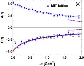
5 Analysis of MIT lattice data at MeV.
The recent MIT lattice data [1] yield and in the space like region at an unphysical fixed pion mass MeV. From Eq. (8) we have constructed by simply adding errors in and in quadrature.333This assumes uncorrelated and , i.e. , and yields . Alternatively, one may naturally assume that spin-0 and spin-2 are independent degrees of freedom, and are uncorrelated, such that , in which case . However, the results of the two scenarios differ little, since and the relative factor of 9 in with respect to dominates the errors. The single resonance model is
| (20) |
The fit yields and , with for 49 data points.444The quality of the scalar channel data does not yet allow for a detailed analysis, which without further independent input easily incurs in overfitting with the proliferation of parameters. For instance, adding a prefactor , one gets GeV and with , but with a large correlation between and . Likewise, adding an term also suffers from overfitting.
6 Pion mass effects and the chiral low energy constants
In QCD, there are only two parameters: and the quark masses , which are mapped onto MeV and MeV for the simple two flavor case with equal assumed all over. The MIT lattice data are at the unphysical and fixed pion mass value of MeV (and, consequently, at MeV), so one should account for this effect in comparison to experimental data. The only known way to connect these unphysical data to the real MeV world is by means of PT, since the corresponding LECs at a given renormalization scale are independent of the pion mass. Conventionally, this scale is taken to be about GeV, and transforming the MIT data to the experimental pion mass MeV is in general model dependent, except in the low momentum region where PT can be applied. For the absorptive part, one gets perturbatively
| (21) |
and hence (for given fixed and values)
| (22) | |||||
| (23) |
From these expressions we get
| (24) |
Fitting Eq. (22) to the MIT lattice data for yields and , with the correlation at GeV (and GeV).
These expressions are good enough to fit to NLO accuracy fixed pion mass data. However, in order to relate different pion masses a mass independent renormalization scheme is needed, such as , as done in [11]. The PT expression for the SEM with the gravitational LECs, , is
| (25) | |||||
| (26) | |||||
| (27) | |||||
where means the trace in the flavor space. The expansion for the flat space reads , which contains the widely known coefficients. A direct comparison of Eq. (22) to Ref. [11] yields the identification
| (28) |
where the and threshold effects have been neglected. The coefficients are scale independent, whereas are independent on the pion mass. Thus , and from the MIT lattice data and (28) we obtain and
| (29) |
with the strong correlation . Matching the monopole expression of Eq. (20) to the PT results for MeV yields MeV and MeV.
| Ref. | |||||||
|---|---|---|---|---|---|---|---|
| DGL [15] | 0.50 | 1.01 | 5.77 | 0.50 | 1.01 | 5.77 | |
| CCP [16] | 0.46 | 0.97 | 5.91 | 0.53 | 1.01 | 5.96 | |
| BPTZ [17] | 0.34 | 0.79 | 5.06 | 0.61 | 0.95 | 5.27 | |
| [9] | 0.0392 | 0.91(6) | 4.4(4) | ||||
| [9] | 0.40(7) | 1 | 5.2(9) |
7 Sum rules revisited
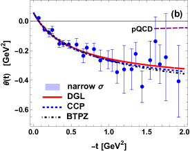
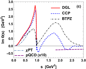
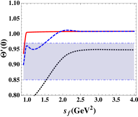
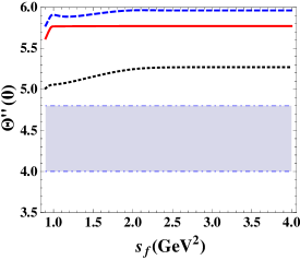
Phenomenological studies of the coupled-channel unitary approach based on the Omnès-Muskhelishvili equations indeed confirm a zero of at about [15, 16, 17] and a certain oscillating pattern beyond that scale, see Fig. 1 (c). Despite their differences in the time-like region (Fig. 1 (c)), they are hardly distinguishable in the space like region (Fig. 1 (b)), where they strongly resemble the monopole fit with MeV, confirming the mentioned space-like insensitivity to detailed time-like physics. From the exact dispersion relations
| (30) |
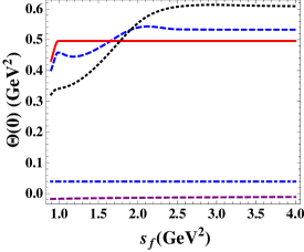
for , which are sum rules for derivatives at the origin, increasingly independent on high energies. The contributions up to the upper limit are listed in Table 1. In Fig. 2 we plot the values of , , and as functions of the matching point between the coupled channel solution and the LO-pQCD. As we see, the mass sum rule is badly violated, whereas the and sum rules overhit the PT estimate, suggesting that there is a significant missing negative contribution in the higher energy tail before pQCD sets in.555This is similar to the pion charge form factor determined from the experimental data for [18], which fulfills similar sum rules as ; the large violations happen with pQCD to NNLO [19].
Among the many possibilities, we assume here a simple power model in the intermediate range which resembles the asymptotic behavior of a radial Regge spectrum [20]
| (31) |
The discussed sum rule violations correspond to taking . Instead, in the limit we may neglect the pQCD tail and the sum rules for a sharp resonance contribution plus Eq. (31) read
| (32) |
Then , in agreement with the phenomenological findings (see Fig. 1 (c)). For simplicity, the scale is chosen, since (in the DGL scenario). Taking GeV and we get and , in agreement with PT (see Table 1). This power falls off faster than the pQCD contribution, Eq. (17), and will eventually intersect when at the large scale (see also Re.([20]), such that in practice in this model the pQCD expression does not contribute significantly to the sum rules. We refrain here from a thorough analysis, as the model is only schematic. However, at face value it shows that despite of reinforcing the usefulness of the meson dominance idea in the intermediate energy region, the inclusion of rigorous QCD sum rules for the form factors calls for a negative spectral strength much larger than a direct extrapolation of pQCD to any energy above GeV. Simple models compatible with low energy phenomenology and fulfilling the sum rules suggests a delayed onset of pQCD, moved to very high energies.
Acknowledgments
We thank Pablo Sánchez Puertas for discussions and Dimitra Pefkou for correspondence.
References
- [1] D.C. Hackett, P.R. Oare, D.A. Pefkou and P.E. Shanahan, Gravitational form factors of the pion from lattice QCD, Phys. Rev. D 108 (2023) 114504 [2307.11707].
- [2] K. Raman, Gravitational form-factors of pseudoscalar mesons, stress-tensor-current commutation relations, and deviations from tensor- and scalar-meson dominance, Phys. Rev. D 4 (1971) 476.
- [3] H. Pagels, Energy-momentum structure form factors of particles, Phys. Rev. 144 (1966) 1250.
- [4] M.V. Polyakov and P. Schweitzer, Forces inside hadrons: pressure, surface tension, mechanical radius, and all that, Int. J. Mod. Phys. A 33 (2018) 1830025 [1805.06596].
- [5] S. Kumano, Q.-T. Song and O.V. Teryaev, Hadron tomography by generalized distribution amplitudes in pion-pair production process and gravitational form factors for pion, Phys. Rev. D 97 (2018) 014020 [1711.08088].
- [6] QCDSF, UKQCD collaboration, The Spin structure of the pion, Phys. Rev. Lett. 101 (2008) 122001 [0708.2249].
- [7] W. Broniowski and E. Ruiz Arriola, Gravitational and higher-order form factors of the pion in chiral quark models, Phys. Rev. D 78 (2008) 094011 [0809.1744].
- [8] P. Masjuan, E. Ruiz Arriola and W. Broniowski, Meson dominance of hadron form factors and large- phenomenology, Phys. Rev. D 87 (2013) 014005 [1210.0760].
- [9] W. Broniowski and E. Ruiz Arriola, Gravitational form factors of the pion and meson dominance, 2405.07815.
- [10] V.A. Novikov and M.A. Shifman, Comment on the psi-prime — J/psi pi pi Decay, Z. Phys. C 8 (1981) 43.
- [11] J.F. Donoghue and H. Leutwyler, Energy and momentum in chiral theories, Z. Phys. C 52 (1991) 343.
- [12] X.-B. Tong, J.-P. Ma and F. Yuan, Gluon gravitational form factors at large momentum transfer, Phys. Lett. B 823 (2021) 136751 [2101.02395].
- [13] X.-B. Tong, J.-P. Ma and F. Yuan, Perturbative calculations of gravitational form factors at large momentum transfer, JHEP 10 (2022) 046 [2203.13493].
- [14] W.-Y. Liu, E. Shuryak and I. Zahed, Pion gravitational form factors in the QCD instanton vacuum. II, Phys. Rev. D 110 (2024) 054022 [2405.16269].
- [15] J.F. Donoghue, J. Gasser and H. Leutwyler, The Decay of a Light Higgs Boson, Nucl. Phys. B 343 (1990) 341.
- [16] A. Celis, V. Cirigliano and E. Passemar, Lepton flavor violation in the Higgs sector and the role of hadronic -lepton decays, Phys. Rev. D 89 (2014) 013008 [1309.3564].
- [17] P.J. Blackstone, J. Tarrús Castellà, E. Passemar and J. Zupan, Hadronic Decays of a Higgs-mixed Scalar, 2407.13587.
- [18] E. Ruiz Arriola and P. Sanchez-Puertas, Phase of the electromagnetic form factor of the pion, Phys. Rev. D 110 (2024) 054003 [2403.07121].
- [19] P. Sanchez-Puertas and E. Ruiz Arriola, The electromagnetic pion form factor and its phase, in 10th International Conference on Quarks and Nuclear Physics, 10, 2024 [2410.17804].
- [20] E. Ruiz Arriola and W. Broniowski, Pion electromagnetic form factor, perturbative QCD, and large-N(c) Regge models, Phys. Rev. D 78 (2008) 034031 [0807.3488].