Integral-integral affine geometry, geometric quantization, and Riemann–Roch

Abstract.

We give a simple proof that, for a pre-quantized compact symplectic manifold with a Lagrangian torus fibration, its Riemann–Roch number coincides with its number of Bohr–Sommerfeld fibres. This can be viewed as an instance of the “independence of polarization” phenomenon of geometric quantization. The base space for such a fibration acquires a so-called integral-integral affine structure. The proof uses the following simple fact, whose proof is trickier than we expected: on a compact integral-integral affine manifold, the total volume is equal to the number of integer points.

1. Introduction

The context of this paper lies within geometric quantization. “Quantization” is the art of getting from a mathematical model for a classical mechanical system to a mathematical model for a corresponding quantum mechanical system; geometric quantization does so using the geometry of the classical system. Recipes for geometric quantization rely on additional auxiliary structure, called a polarization, which is heuristically a “choice of half the variables,” analogous to how classical phase space has both position and momentum coordinates, but quantum “wave functions” are functions of position only. A central theme in geometric quantization, of which there is ample evidence and only partial understanding, is “independence of polarization,” by which certain features of the quantized space are independent of the choice of polarization.

The following result can be viewed as an instance of this “independence of polarization” phenomenon (see Section 2 for details and definitions):

Let $(M,\omega)$ be a compact symplectic manifold, let $\pi\colon M\to B$ be a (regular) Lagrangian fibration, and let $L\to M$ be a prequantization line bundle. Then the Riemann–Roch number of $(M,\omega)$ is equal to the number of Bohr–Sommerfeld fibres of $L\to M\to B$.

This result is Theorem 2.2 below, to which we refer as the “Upstairs Theorem”. In principle, this result has been known to experts for many years; it appeared as Corollary 6.12 in the paper [FFY] by Fujita, Furuta, and Yoshida, who in turn attribute it to Andersen’s paper [And]. In both cases, the proof passes through a more complicated theorem, and our original purpose in writing this paper was to give a simple, direct proof of this result. (For more details on the relation of our work with the existing literature, see Section 10.)

Our proof of the Upstairs Theorem relies on the following result from “integral-integral affine geometry” (see Section 3 for details and definitions), which on the surface has nothing to do with geometric quantization:

Let $B$ be a compact integral-integral affine manifold. Then the volume of $B$ is equal to the number of integral points in $B$.

This result is Theorem 3.1 below, to which we refer as the “Downstairs Theorem”.

We were not able to find this result in the literature, and in trying to write down a simple proof, we were surprised to find that it was trickier than expected. For a while, we toyed with the idea of flipping the logic: deducing the Downstairs Theorem from the Upstairs Theorem and changing the title of our paper to “An inappropriate proof, using geometric quantization, of a simple fact from integral-integral affine geometry.” Eventually, it turned out that we do not need geometric quantization to prove the Downstairs Theorem. But we do use Lagrangian torus fibrations, and a not-entirely-obvious cohomological argument (see Theorems 7.6 and 8.2). These arguments may be known to experts (see Section 10), but we were not able to find an explicit proof in the literature.

One thing that makes the Downstairs Theorem interesting is that, although the base $B$ is compact, we do not know if its affine connection is geodesically complete. This is a special case of the Markus conjecture; see §3.

An alternative approach to the Downstairs Theorem, suggested to us by Yiannis Loizides, is to decompose $B$ into simple integral convex polytopes $B_{i}$ and to apply to each $B_{i}$ the exact Euler-MacLaurin formula of [KSW]. Such an approach might not be simpler than ours, but it may lead to a more general result, in which we allow $\pi\colon M\to B$ to be a completely integrable system with elliptic (“locally toric”) singularities over a manifold-with-corners $B$. Such systems are studied in [Mo] and [FM].

The organization of this paper is as follows. In Section 2, we state our Upstairs Theorem as Theorem 2.2 and give some necessary definitions. In Section 3, we recall facts about integral affine structures and define integral-integral affine structures, leading to the statement of our Downstairs Theorem in Theorem 3.1. In Section 4, we recall how a Lagrangian torus fibration induces an integral affine structure on its base, and we show — using “enhanced Arnol’d–Liouville charts” — how a prequantized Lagrangian torus fibration induces an integral-integral affine structure on its base. In Section 5, we give our short proof of the Upstairs Theorem modulo the Downstairs Theorem. In Section 6, we describe the integral lattice in $TB$ and period lattice in $T^{*}B$ when $B$ is integral affine, and the affine lattice in $TB$ when $B$ is integral-integral affine. In Section 7, we introduce local torus actions, and we show that, with a local torus action, every de Rham cohomology class is represented by an invariant form. Finally, in Section 8 we use local torus actions and the aforementioned cohomological argument to prove the Downstairs Theorem. Section 9 contains a discussion of dual torus fibrations that is not necessary for our proof but that provides geometric context. And in Section 10 we comment on the connection of our work to some existing literature.

Here is a list of the two main theorems, and the lemmas that allow us to deduce the Upstairs Theorem from the Downstairs Theorem.

Theorem 2.2 (Upstairs):	$\operatorname{RR}(M)=|\text{BS}|$
Theorem 3.1 (Downstairs):	$\operatorname{vol}(B)=|B_{\mathbb{Z}}|$
Lemma 4.4:	$\operatorname{vol}(M)=\operatorname{vol}(B)$
Lemma 4.12:	$\text{BS}=B_{\mathbb{Z}}$
Lemma 5.1:	$\operatorname{RR}(M)=\operatorname{vol}(M)$

Acknowledgements

We are grateful for discussions with Bill Goldman, Yiannis Loizides, Oliver Goertches, Alex Lubotzky, Yuichi Nohara, and Louis Ioos.

Yael Karshon and Mark Hamilton acknowledge the support of the Natural Sciences and Engineering Research Council of Canada (NSERC). Yael Karshon’s research is also partly funded by the United-States – Israel Binational Science Foundation. Takahiko Yoshida’s work is supported by Grant-in-Aid for Scientific Research (C) 15K04857 and 19K03479.

2. Upstairs — geometric quantization

In this section we give the definitions necessary to state our “Upstairs Theorem,” as well as provide some context, and state the theorem as Theorem 2.2. We prove this theorem in Section 5, assuming our “Downstairs Theorem,” which we state in Section 3 and prove in Section 8.

For our purposes, geometric quantization is a recipe that associates to a compact symplectic manifold $(M,\omega)$ a finite dimensional vector space $\mathcal{Q}(M)$ (or more generally a virtual vector space, i.e., a formal difference of two vector spaces), which is constructed from sections of a particular complex line bundle $L\to M$. One part of the recipe of geometric quantization is a “polarization,” of which the most commonly considered types are as follows. A Kähler polarization is given by a compatible complex structure on $M$, which makes $L$ into a holomorphic line bundle; then $\mathcal{Q}(M)$ is the space of holomorphic sections of $L$. A real polarization is given by a foliation of $M$ into Lagrangian submanifolds, usually assumed to be the fibres of a fibration  $\pi\colon M\to B$. In this case, $\mathcal{Q}(M)$ is constructed from sections of $L\to M$ that are covariant constant along the fibres of $\pi$, and can typically be described in terms of Bohr–Sommerfeld fibres, defined further below. One natural question that arises is “independence of polarization”: Given two polarizations on the same $M$, are the resulting quantizations the same?

Riemann–Roch numbers

Recall that the Todd class associates to each rank $n$ complex vector bundle $E\to M$ a cohomology class of mixed degree on $M$, associated through the Chern–Weyl recipe to the Taylor series at $0$ of the function $\prod_{i=1}^{n}\frac{x_{i}}{1-e^{-x_{i}}}$. Given a compact symplectic manifold $(M,\omega)$, we define its Riemann–Roch number by

(2.1) $${}\operatorname{RR}(M,\omega)=\int_{M}\exp(\omega)\operatorname{Todd}(TM,J),$$

where $J$ is any compatible almost complex structure. (Different choices of compatible almost complex structures $J$ give isomorphic complex vector bundles $(TM,J)$, hence the same Todd class.)

We can interpret the Riemann–Roch number as the dimension of a quantization of $(M,\omega)$. When $\omega$ is the curvature of a complex Hermitian line bundle $L\to M$, we can declare the quantization space to be the virtual vector space obtained as the formal difference of the kernel and cokernel of the corresponding Dirac–Dolbeault operator. See, e.g., Duistermaat’s book [D1, Chapter 15]. The Riemann–Roch number then computes the index of this operator, i.e., the difference of the dimensions of the kernel and cokernel; in particular, it’s an integer. In the presence of a compatible complex structure on $M$, the line bundle $L\to M$ becomes holomorphic, and this virtual vector space coincides with the alternating sum of the cohomologies of the sheaf of holomorphic sections of $L$. When the higher cohomology vanishes (such as when we pass to $L^{\otimes k}$ for sufficiently large $k$), we are left with the space of holomorphic sections, and in this case the Riemann–Roch number gives the dimension of the space of holomorphic sections, which can be viewed as the dimension of the quantization $\mathcal{Q}(M)$.

Bohr–Sommerfeld sets

Let $(M,\omega)$ be a symplectic manifold, and let $L\to M$ be a prequantization line bundle with connection, i.e., $L$ is a complex Hermitian line bundle, equipped with a connection whose curvature is $\omega$. For any Lagrangian submanifold $N$ of $M$, the pullback of $L$ to $N$ is a line bundle with a flat connection. The Lagrangian $N$ is Bohr–Sommerfeld if this connection is trivializable. Equivalently, $N$ is Bohr–Sommerfeld if the holonomy of the prequantization connection is trivial around every loop in $N$. Given a Lagrangian fibration $\pi\colon M\to B$, the corresponding Bohr–Sommerfeld points are those points of $B$ whose preimage in $M$ is a Bohr–Sommerfeld Lagrangian; the set of such points is the Bohr–Sommerfeld set, which we denote BS.

In this case the quantization of $M$ with respect to the real polarization defined by the Lagrangian fibration $\pi$ is constructed from sections of $L\to M$ that are covariant constant along the fibres of $\pi$. There are several recipes for doing so; as one example, Śniatycki [Sn] constructs this quantization as a cohomology group of the sheaf of such sections. (See §3 of [H] for a fuller discussion of quantization using a real polarization.) Typically, we can interpret the Bohr–Sommerfeld set as indexing a set of basis elements of a quantization of $(M,\omega)$, so that the number of Bohr–Sommerfeld points in $B$ gives the dimension of the quantization of $M$. For the purposes of this paper, we define the dimension of the Bohr–Sommerfeld quantization in this way.

The main theorem of this paper is the following:

2.2 Theorem (“Upstairs theorem”).

Let $(M,\omega)$ be a compact symplectic manifold, let $\pi\colon M\to B$ be a (regular) Lagrangian fibration, and let $L\to M$ be a prequantization line bundle. Then the Riemann–Roch number of $M$ is equal to the number of Bohr–Sommerfeld fibres of $L\to M\to B$:

$$\operatorname{RR}(M,\omega)=\lvert\text{BS}\,\rvert.$$

Theorem 2.2 can be viewed as an instance of “independence of polarization,” in the sense that the vector space that is associated to $L\to M$ through Dirac–Dolbeault quantization has the same dimension as the vector space that is associated to $L\to M$ through Bohr–Sommerfeld quantization. In Section 5 we will reduce Theorem 2.2 to Theorem 3.1; we will prove Theorem 3.1 in Section 8.

One corollary of the arguments leading to Theorem 2.2 is that different Lagrangian torus fibrations on a symplectic manifold $M$ have the same number of Bohr–Sommerfeld points:

2.3 Corollary.

Let $(M,\omega)$ be a compact symplectic manifold, let $L\to M$ be a prequantization line bundle, and let $\pi_{1}\colon M\to B_{1}$ and $\pi_{2}\colon M\to B_{2}$ be Lagrangian fibrations, with corresponding Bohr–Sommerfeld sets $\text{BS}_{1}$ and $\text{BS}_{2}$. Then $\lvert\text{BS}_{1}\rvert=\lvert\text{BS}_{2}\rvert$.

Proof.

By putting together Lemma 4.4, Lemma 4.12, and Theorem 3.1, we see that the number of Bohr–Sommerfeld points in either $B_{1}$ or $B_{2}$ equals the volume of $M$. ∎

In the context of quantization, this means that two real polarizations on the same manifold $(M,\omega)$ will yield Bohr–Sommerfeld quantizations of the same dimension. For example, see the discussion of different real polarizations on the Kodaira–Thurston manifold in [HM].

We are grateful to Jonathan Weitsman for the following observation, which follows by the same argument as Corollary 2.3:

2.4 Corollary.

Let $(M,\omega)$ be a compact symplectic manifold, and $\pi\colon M\to B$ a (regular) Lagrangian fibration. Let $L_{1}\to M$ and $L_{2}\to M$ be prequantization line bundles with corresponding Bohr–Sommerfeld sets $BS_{1}$ and $BS_{2}$. Then $\lvert\text{BS}_{1}\rvert=\lvert\text{BS}_{2}\rvert$.

If a prequantizable symplectic manifold $M$ is simply-connected, then it has a unique prequantization line bundle up to equivalence. (Indeed, if $L$ and $L^{\prime}$ are prequantization line bundles, then $L^{-1}\otimes L^{\prime}$ is a line bundle with a flat connection, which is trivial if $H_{1}(M)=0$. See [K, Theorem 2.2.1].) Corollary 2.4 shows that in the case of Lagrangian torus fibrations (which typically have $H_{1}\neq 0$), the (dimension of the) real quantization is independent of the choice of $L$. A similar result will hold for any quantization whose dimension is given by the Riemann–Roch number.

We are similarly grateful to Daniele Sepe for the following observation, which says that the quantization is unchanged by adding a “magnetic term”:

2.5 Corollary.

Let $(M,\omega)$ be a compact symplectic manifold, $\pi\colon M\to B$ a (regular) Lagrangian fibration, and $L\to M$ a prequantization line bundle. Suppose $\beta$ is a closed integral 2-form on $B$, and suppose $L^{\prime}\to M$ is a prequantization line bundle with respect to $\omega+\pi^{*}\beta$. Then the Bohr–Sommerfeld sets of $L$ and $L^{\prime}$ have the same number of points.

Proof.

If $L^{\prime}=L\otimes\pi^{*}L_{B}$ where $L_{B}\to B$ is a line bundle with connection whose curvature is $\beta$ (which exists by [K, Theorem 2.1.1]), then $L^{\prime}$ is a prequantization of $(M,\omega+\pi^{*}\beta)$, and its Bohr–Sommerfeld set is equal to that of $L$. Together with Corollary 2.4, we obtain the result for general $L^{\prime}$. ∎

3. Downstairs — integral-integral affine geometry

In this section, we review some facts about integral affine structures, and we define the notion of “integral-integral affine structure”, leading to the statement of our Downstairs Theorem, Theorem 3.1.

Affine structures

An affine map on $\mathbb{R}^{n}$ is a map of the form $x\mapsto Ax+b$ for some $A\in\operatorname{GL}_{n}(\mathbb{R})$ and $b\in\mathbb{R}^{n}$. An affine atlas on a manifold $B$ is a collection of charts $\phi_{\alpha}\colon U_{\alpha}\to\Omega_{\alpha}\subset\mathbb{R}^{n}$ whose domains $U_{\alpha}$ cover $B$ and whose transition maps $\phi_{\beta}\circ\phi_{\alpha}^{-1}$ are locally affine. An affine structure is a maximal affine atlas. Such a structure induces a torsion-free flat connection on $TB$, by declaring the coordinate vector fields to be horizontal.

Integral affine structures

An integral affine map on $\mathbb{R}^{n}$ is a map of the form $x\mapsto Ax+b$ for some $A\in\operatorname{GL}_{n}(\mathbb{Z})$ and $b\in\mathbb{R}^{n}$. Equivalently, it is an affine map whose linear part takes the lattice $\mathbb{Z}^{n}$ onto itself. An integral affine atlas on a manifold $B$ is a collection of charts $\phi_{\alpha}\colon U_{\alpha}\to\Omega_{\alpha}\subset\mathbb{R}^{n}$ whose domains cover $B$ and whose transition maps $\phi_{\beta}\circ\phi_{\alpha}^{-1}$ are locally integral affine. An integral affine structure is a maximal integral affine atlas. Such a structure induces a smooth measure on $B$, coming from the usual Lebesgue measure on $\mathbb{R}^{n}$. We can then refer to the total volume, $\operatorname{vol}(B)$.

Integral-integral affine structures

An integral-integral affine map of $\mathbb{R}^{n}$ is a map of the form $x\mapsto Ax+b$ for some $A\in\operatorname{GL}_{n}(\mathbb{Z})$ and $b\in\mathbb{Z}^{n}$. Equivalently, it is an affine map that takes the lattice $\mathbb{Z}^{n}$ onto itself. An integral-integral affine atlas on a manifold $B$ is a collection of charts $\phi_{\alpha}\colon U_{\alpha}\to\Omega_{\alpha}\subset\mathbb{R}^{n}$ whose domains cover $B$ and whose transition maps $\phi_{\beta}\circ\phi_{\alpha}^{-1}$ are locally integral-integral affine. An integral-integral affine structure is a maximal integral-integral affine atlas. Such a structure determines a subset $B_{\mathbb{Z}}$ of $B$, defined as the set of those points $b\in B$ that are sent to $\mathbb{Z}^{n}$ by some, hence all, integral-integral charts that contain $b$. We call it the set of integral points in $B$.

Examples

A prototypical example of an integral-integral affine manifold is the quotient of $\mathbb{R}^{n}$ by a group $\Gamma$ of integral-integral affine transformations that acts freely and properly. Specific examples include the torus, where $\Gamma$ is generated by the maps

$$x_{1}\mapsto x_{1}+1,\quad\ldots,\quad x_{n}\mapsto x_{n}+1;$$

the Klein bottle, where $n=2$ and $\Gamma$ is generated by the maps

$$x_{1}\mapsto x_{1}+1,\quad(x_{1},x_{2})\mapsto(-x_{1},x_{2}+1);$$

and Kodaira-Thurston-like manifolds, with $\Gamma$ generated by the maps

$$(x_{1},x_{2},x_{3})\mapsto(x_{1}+x_{2},x_{2},x_{3}+1),\quad\text{ and }\quad x_{j}\mapsto x_{j}+1\text{ for all $j\neq 3$}.$$

We ask:

Does every compact integral-integral affine manifold arise as a quotient of $\mathbb{R}^{n}$ by a free and proper action of a discrete group of integral-integral affine maps?

This appears to be an open question. It is a special case of the Markus conjecture, which posits that if a closed affine manifold possesses an atlas whose transition maps all have $\det A=\pm 1$ then it is geodesically complete. For a survey of the Markus conjecture, see [Go, Chap. 11].

Volume and lattice points

Recall that an integral affine structure on a manifold $B$ determines a smooth measure on $B$, and an integral-integral affine structure also determines a notion of “integer points” in $B$. We are now ready to state the result in “integral-integral affine geometry” that we will need in our proof of Theorem 2.2:

3.1 Theorem (“Downstairs theorem”).

Let $B$ be a compact integral-integral affine manifold. Then the volume of $B$ is equal to the number of integral points in $B$:

$$\operatorname{vol}(B)=\lvert B_{\mathbb{Z}}\rvert.$$

We will prove this theorem in Section 8.

4. Arnol’d–Liouville

We begin this section by recalling some properties of proper Lagrangian fibrations. First, we recall the Arnol’d–Liouville theorem. Next, we recall that a proper Lagrangian fibration induces on its base an integral affine structure, whose induced measure is the push-forward of Liouville measure. We then prove an “enhanced Arnol’d–Liouville Theorem,” giving a local model for a pre-quantized proper Lagrangian fibration. Finally, we show that a pre-quantized proper Lagrangian fibration induces on its base an integral-integral affine structure, whose lattice points coincide with the Bohr–Sommerfeld points. This provides preparation for Section 5, where we prove our Upstairs Theorem (“$\operatorname{RR}=|\text{BS}|$”), assuming our Downstairs Theorem (“$\operatorname{vol}(B)=|B_{\mathbb{Z}}|$”). We defer the proof of our Downstairs Theorem to Section 8.

Lie tori and smooth tori

We will encounter some tori. For a fixed $n$, we will use $\mathbb{T}^{n}$ to denote the standard torus $(S^{1})^{n}$. To avoid ambiguity, we will use the terms Lie torus for a Lie group that is isomorphic (as a Lie group) to $\mathbb{T}^{n}$ for some $n$, and smooth torus for a manifold that is diffeomorphic to $\mathbb{T}^{n}$ for some $n$.

Arnol’d–Liouville

A map from a symplectic manifold $(M,\omega)$ to a manifold $B$ is a Lagrangian fibration if it is a (locally trivializable) fibre bundle whose fibres are Lagrangian submanifolds of $M$. It is a Lagrangian torus fibration if, additionally, its fibres are (smooth) tori. The Arnol’d–Liouville theorem implies that every proper Lagrangian fibration with connected fibres is a Lagrangian torus fibration. Moreover, this theorem gives local “action-angle coordinates” on such fibrations. We express such coordinates in terms of what we call “Arnol’d–Liouville charts.”

4.1 Definition.

Given a proper Lagrangian fibration $\pi\colon(M,\omega)\to B$ with connected fibres, an Arnol’d–Liouville chart consists of:

• a connected open subset $U$ of $B$

• a diffeomorphism of $U$ with an open subset $\Omega$ of $\mathbb{R}^{n}$

• a lifting of this diffeomorphism to a symplectomorphism from $\pi^{-1}(U)$ to $\Omega\times\mathbb{T}^{n}$ with the standard symplectic form $\sum dx_{j}\wedge dt_{j}$, with $t_{j}$ mod $1$ coordinates on the $\mathbb{T}^{n}$ factor.

We refer to such a space $\Omega\times\mathbb{T}^{n}$, with its standard symplectic form, as an Arnol’d–Liouville model.

4.2 Theorem (Arnol’d–Liouville).

Every proper Lagrangian fibration with connected fibres can be covered by Arnol’d–Liouville charts.

Proof.

This theorem is a reformulation of the Arnol’d–Liouville Theorem in the case that the fibres are compact. See, e.g., [Arn2, §49–50], [MM, lemma in §3], [D2]. ∎

4.3 Lemma.

Let

$$\Omega\times\mathbb{T}^{n}\to\Omega^{\prime}\times\mathbb{T}^{n}\quad,\quad(x,t)\mapsto(x^{\prime},t^{\prime})$$

be an isomorphism of Arnol’d–Liouville models, i.e., a fibre-preserving symplectomorphism. Then its components have the form

$$x^{\prime}=Ax+b,\qquad t^{\prime}=A^{-T}t+g(x)$$

for some $A\in\operatorname{GL}_{n}(\mathbb{Z})$,  $b\in\mathbb{R}^{n}$, and $g\colon\Omega\to\mathbb{T}^{n}$, where $A^{-T}$ denotes the inverse transpose of the matrix $A$.

(Note that our definition of an Arnol’d–Liouville chart assumes that $\Omega$ is connected.)

Proof of Lemma 4.3.

This follows from a direct computation (see for example Lemma 2.1 in [Se]). ∎

Lagrangian torus fibration induces integral affine structure

4.4 Lemma.

Let $\pi\colon(M,\omega)\to B$ be a $2n$-dimensional Lagrangian torus fibration. Then the set of maps $U\to\Omega$ that arise from Arnol’d–Liouville charts is an integral affine atlas on $B$. Moreover, the induced measure on $B$ coincides with the push-forward to $B$ of Liouville measure on $M$. In particular, if $M$ is compact, then $\operatorname{vol}(M)=\operatorname{vol}(B)$ (with respect to these measures).

Proof.

By Theorem 4.2, the domains of the maps $U\to\Omega$ are an open cover of $B$. By Lemma 4.3, the transition maps of this cover are integral affine. By a direct computation in local coordinates in any Arnol’d–Liouville chart, the push-forward of Liouville measure on $M$ is the measure on $B$. ∎

Enhanced Arnol’d–Liouville

In this subsection we will give a local model for a prequantized proper Lagrangian fibration, and prove an “enhanced” Arnol’d–Liouville Theorem (Theorem 4.8).

4.5 Definition.

Given a prequantized Lagrangian torus fibration, i.e., a Lagrangian torus fibration $\pi\colon(M,\omega)\to B$, equipped with a Hermitian line bundle $p\colon L\to M$ with connection $\nabla$ whose curvature is $\omega$, an enhanced Arnol’d–Liouville chart consists of:

• a connected open subset $U$ of $B$

• a diffeomorphism of $U$ with an open subset $\Omega$ of $\mathbb{R}^{n}$

• a lifting of this diffeomorphism to a symplectomorphism from $\pi^{-1}(U)$ to $\Omega\times\mathbb{T}^{n}$ with the standard symplectic form $\sum dx_{j}\wedge dt_{j}$, with $t_{j}$ mod $1$ coordinates on the $\mathbb{T}^{n}$ factor.

• a lifting of this symplectomorphism to an isomorphism of Hermitian line bundles from $p^{-1}(\pi^{-1}(U))$ to $\Omega\times\mathbb{T}^{n}\times\mathbb{C}$ that intertwines $\nabla$ with $d-2\pi i\sum x_{j}\,dt_{j}$.

We refer to such a complex line bundle $\Omega\times\mathbb{T}^{n}\times\mathbb{C}$ over $\Omega\times\mathbb{T}^{n}$, with the standard symplectic form on its base and with the covariant derivative $d-2\pi i\sum x_{j}\,dt_{j}$, as an enhanced Arnol’d–Liouville model.

4.6 Remark.

There are various different conventions in the literature for curvature and prequantization; ours are as follows. A 1-form $\alpha$ represents a connection with respect to a local trivialization if, in this local trivialization, the covariant derivative is $d+2\pi i\alpha$. The curvature of the connection is then $-d\alpha$. A prequantization line bundle has a connection with curvature equal to the symplectic form. Thus, in an enhanced Arnol’d–Liouville chart, the 1-form representing the connection is $-\sum x_{j}\,dt_{j}$ and the curvature is $\sum dx_{j}\wedge dt_{j}$.

Our convention for a 1-form representing a connection agrees with Kostant’s paper [K] (see Equation 1.4.3 on p. 98) and differs from Woodhouse’s book [W] by a sign and a factor of $2\pi$ (see [W, §A.3]). Given the 1-form, our convention for the curvature of a connection has opposite sign from [K] (see p. 104, after Prop. 1.6.1) and agrees with the conventions in [GGK] (see Lemma A.3, p. 169) and [W] (see §A.3). Given the curvature, our convention for the prequantization data agrees with [K] (see §4 on p. 165]) and with [Sn], and differs from [W] by a factor of $\hbar$ (see [W, p. 158]).

$\diamond$

4.7 Lemma.

Let $\Omega\times\mathbb{T}^{n}\times\mathbb{C}$ be an enhanced Arnol’d–Liouville model, with coordinates $(x_{1},\ldots,x_{n},\linebreak t_{1},\ldots,t_{n},z)$ with $t_{j}$ taken mod 1. For any fixed $x\in\Omega$ and any $k\in\{1,\ldots,n\}$, let $\gamma_{k}$ be the loop in $\{x\}\times\mathbb{T}^{n}$ corresponding to one cycle in the $t_{k}$ variable. Then the holonomy around $\gamma_{k}$ is $e^{2\pi ix_{k}}$.

Proof.

We can take $\gamma_{k}$ to be given by $x_{j}(s)=x_{j}(0)$ for all $j$,  $t_{j}(s)=0$ for $j\neq k$, and $t_{k}(s)=s$, for $0\leq s\leq 1$. Because the covariant derivative is $d-2\pi i\sum x_{j}\,dt_{j}$, the horizontal lifts of $\gamma_{k}$ are then given by $z(s)=e^{2\pi isx_{k}}z(0)$. ∎

4.8 Theorem (Enhanced Arnol’d–Liouville).

Every prequantized Lagrangian torus fibration can be covered by enhanced Arnol’d–Liouville charts.

Proof.

By Theorem 4.2, every point in the symplectic manifold has a neighbourhood that can be identified with an Arnol’d–Liouville model $\Omega\times\mathbb{T}^{n}$. After shrinking the neighbourhood, we may assume that $\Omega$ is contractible. Thus, it is enough to prove that, for any Arnol’d–Liouville model $\Omega\times\mathbb{T}^{n}$ with $\Omega$ a contractible open subset of $\mathbb{R}^{n}$, any prequantization line bundle over it is isomorphic to an enhanced Arnol’d–Liouville model.

Fix such an Arnol’d–Liouville model and a prequantization line bundle

$$(L,\left<,\right>,\nabla)\to(\Omega\times\mathbb{T}^{n},\sum dx_{j}\wedge dt_{j}).$$

We first prove that $(L,\left<,\right>)$ is trivializable as a complex Hermitian line bundle. Fix $q\in\Omega$. Because $\Omega$ is contractible, it is enough to show that the complex Hermitian line bundle $L|_{\{q\}\times\mathbb{T}^{n}}$ is trivializable. Because the pullback of the curvature $\sum dx_{j}\wedge dt_{j}$ to the fibre $\{q\}\times\mathbb{T}^{n}$ is zero, the pullback connection on $L|_{\{q\}\times\mathbb{T}^{n}}$ is flat. The holonomy of this connection becomes a map

$$\operatorname{hol}\colon\pi_{1}(\mathbb{T}^{n})\to S^{1}.$$

For each $j\in\{1,\ldots,n\}$, let $\gamma_{j}$ be a loop around $\mathbb{T}^{n}$ in the $t_{j}$ coordinate, and choose $h_{j}\in\mathbb{R}$ such that $\operatorname{hol}([\gamma_{j}])=e^{2\pi ih_{j}}$. Then $\lambda:=d-2\pi i\sum h_{j}\,dt_{j}$ defines a connection on the trivial bundle $\mathbb{T}^{n}\times\mathbb{C}\to\mathbb{T}^{n}$ that has the same holonomy. Because a flat bundle is determined up to isomorphism by its holonomy (see Remark 1.12.1 in [K]), $L|_{\{q\}\times\mathbb{T}^{n}}$ is isomorphic to this trivial bundle (with the trivial Hermitian structure and with the flat connection that we constructed). In particular, $(L,\left<,\right>)$ is trivializable as a complex Hermitian line bundle. Fix such a trivialization

$$\psi\colon L\to(\Omega\times\mathbb{T}^{n})\times\mathbb{C}.$$

Since the curvature of $\nabla$ is $\sum dx_{j}\wedge dt_{j}$, the trivialization $\psi$ takes $\nabla$ to $d-2\pi i\sum x_{j}\,dt_{j}+2\pi i\beta$ for some closed 1-form $\beta$ on $\Omega\times\mathbb{T}^{n}$. Since $\Omega$ is contractible, $H^{1}(\Omega\times\mathbb{T}^{n})$ is generated by $dt_{1},\ldots dt_{n}$, so $\beta$ has the form $\sum c_{j}\,dt_{j}+df$ for some constants $c_{j}$ and some function $f$ on $\Omega\times\mathbb{T}^{n}$. Denote $c:=(c_{1},\ldots,c_{n})\in\mathbb{R}^{n}$. Then

$$(x,t,z)\mapsto\bigl{(}x,t,e^{-2\pi if(x,t)}z\bigr{)}$$

defines a bundle automorphism of $\Omega\times\mathbb{T}^{n}\times\mathbb{C}$ that takes $d-2\pi i\sum x_{j}\,dt_{j}+2\pi i\beta$ to $d-2\pi i\sum(x_{j}-c_{j})\,dt_{j}$.

We obtain an isomorphism of $L\to\Omega\times\mathbb{T}^{n}$ with an enhanced Arnol’d–Liouville model by composing $\psi$ with the bundle isomorphism

$$(x,t,z)\mapsto(x-c,t,e^{-2\pi if(x,t)}z).$$

∎

We next prove an “enhanced” analogue of Lemma 4.3, giving the conditions for a map to preserve enhanced Arnol’d–Liouville structures.

4.9 Lemma.

Let

(4.10) $${}\Omega\times\mathbb{T}^{n}\times\mathbb{C}\to\Omega^{\prime}\times\mathbb{T}^{n}\times\mathbb{C}\quad,\quad(x,t,z)\mapsto(x^{\prime},t^{\prime},z^{\prime})$$

be an isomorphism of enhanced Arnol’d–Liouville models, i.e., an isomorphism of line-bundles-with-connection that lifts a fibre-preserving symplectomorphism $\Omega\times\mathbb{T}^{n}\to\Omega^{\prime}\times\mathbb{T}^{n}$. Then its first two components have the form

(4.11) $${}x^{\prime}=Ax+b,\qquad t^{\prime}=A^{-T}t+g(x)$$

for some $A\in\operatorname{GL}_{n}(\mathbb{Z})$, $g\colon\Omega\to\mathbb{T}^{n}$, and $b\in\mathbb{Z}^{n}$.

Proof.

By Lemma 4.3, the first two components have the form (4.11) for some $A\in\operatorname{GL}_{n}(\mathbb{Z})$,  $g\colon\Omega\to\mathbb{T}^{n}$, and $b\in\mathbb{R}^{n}$. It remains to show that $b\in\mathbb{Z}^{n}$.

Writing the coordinates on $\Omega\times\mathbb{T}^{n}\times\mathbb{C}$ as $(x_{1},\ldots,x_{n},t_{1},\ldots,t_{n},z)$, with $t_{j}$ taken mod 1, for any fixed $x\in\Omega$ and any $j\in\{1,\ldots,n\}$, let $\gamma_{j}$ be the loop in $\{x\}\times\mathbb{T}^{n}$ corresponding to one cycle in the $t_{j}$ variable. By Lemma 4.7, the holonomy around $\gamma_{j}$ is $e^{2\pi ix_{j}}$. Since the bundle $\{x\}\times\mathbb{T}^{n}\times\mathbb{C}$ is flat, the holonomy is the same on homologous cycles, and thus gives a homomorphism $\operatorname{hol}_{x}\colon H_{1}(\{x\}\times\mathbb{T}^{n})\to S^{1}$. Let $[\gamma_{j}]$ denote the homology class of $\gamma_{j}$ in $H_{1}(\{x\}\times\mathbb{T}^{n})$.

Similarly, for each $k=1,\ldots,n$ let $\gamma_{k}^{\prime}$ be a loop in a fibre $\{x^{\prime}\}\times\mathbb{T}^{n}$ of $\Omega^{\prime}\times\mathbb{T}^{n}\times\mathbb{C}$ corresponding to one cycle in the $t_{k}^{\prime}$ variable.

Under the map (4.10), the loop $\gamma_{j}$ maps to a loop homologous to $\sum_{k}(A^{-1})_{jk}[\gamma_{k}^{\prime}]$, where as usual $(A^{-1})_{jk}$ denotes the $(j,k)$ entry of the matrix $A^{-1}$. Because the map (4.10) intertwines the connections, the holonomy of $\gamma_{j}$ equals the holonomy of its image under the map (4.11), which is given by

$$\operatorname{hol}_{x^{\prime}}\Bigl{(}\sum_{k}(A^{-1})_{jk}\gamma_{k}^{\prime}\Bigr{)}=\exp\Bigl{(}2\pi i\sum_{k}(A^{-1})_{jk}x_{k}^{\prime}\Bigr{)}.$$

Now $x_{k}^{\prime}=\sum_{i}A_{ki}x_{i}+b_{k}$, so this becomes

$$=\exp\biggl{(}2\pi i\sum_{k}(A^{-1})_{jk}\Bigl{(}\sum_{i}A_{ki}x_{k}+b_{k}\Bigr{)}\biggr{)}$$

$$=\exp\left(2\pi i\biggl{(}\sum_{k,i}(A^{-1})_{jk}(A)_{ki}x_{i}+\sum_{k}(A^{-1})_{jk}b_{k}\biggr{)}\right)$$

$$=\exp\biggl{(}2\pi i\bigl{(}x_{j}+(A^{-1}b)_{j}\bigr{)}\biggr{)}.$$

This will equal $e^{2\pi ix_{j}}$ iff $(A^{-1}b)_{j}$ is an integer. Thus, the coordinate change map will preserve the holonomy of the connection iff $A^{-1}b\in\mathbb{Z}^{n}$. Since $A^{-1}\in\operatorname{GL}_{n}(\mathbb{Z})$, this will be true iff $b\in\mathbb{Z}^{n}$. ∎

Prequantized Lagrangian torus fibration induces integral-integral affine structure

Finally, we show that a prequantization of a proper Lagrangian fibration determines an integral-integral affine structure on the base.

4.12 Lemma.

Let $\pi\colon(M,\omega)\to B$ be a $2n$-dimensional Lagrangian torus fibration with prequantization $(L,\nabla)$. Then the set of maps $U\to\Omega$ that arise from enhanced Arnol’d–Liouville charts is an integral-integral affine atlas on $B$. Moreover, the set of integral points $B_{\mathbb{Z}}$ for this integral-integral affine structure coincides with the Bohr–Sommerfeld set of $(L,\nabla)$ in $B$.

Proof.

By Theorem 4.8, $M$ can be covered by enhanced Arnol’d–Liouville charts, and by Lemma 4.9, the coordinate change map between the bases of two such charts is locally an integral-integral affine transformation. This proves the first claim.

The second claim follows from Lemma 4.7, since a fibre is Bohr–Sommerfeld iff the holonomy is trivial around a set of generators for the fundamental group. ∎

4.13 Remark.

The characterization of the Bohr–Sommerfeld set as points with integer action coordinates has been around for some time. More precisely, once the action coordinates have been fixed so that one Bohr–Sommerfeld point has integer action coordinates, the Bohr–Sommerfeld points in this chart are exactly those points that have integer action coordinates. (See Theorem 2.4 in [GS], and the Remark at the end of §3 of [H] for a brief discussion of the subtleties.) The existence of a globally defined Bohr–Sommerfeld set means that, even if action coordinates cannot be globally defined, it is possible to choose them in such a way that the condition “all action coordinates integers” is well-defined. Such a collection of local action coordinates then gives an integral-integral affine atlas.

5. Proof of “Upstairs Theorem”, assuming “Downstairs Theorem”

In this section, we prove our Upstairs Theorem, “$\operatorname{RR}(M)=|\text{BS}|$” (which is Theorem 2.2), assuming our Downstairs Theorem, “$\operatorname{vol}(B)=|B_{\mathbb{Z}}|$” (which is Theorem 3.1, which we prove in section 8). Originally, we had envisioned that our paper would consist of essentially only this section, before we realized that the Downstairs Theorem is not a triviality.

We begin by proving that, for a compact Lagrangian torus fibration, the Riemann–Roch number is equal to the volume. Here, $[\omega]$ need not be integral.

5.1 Lemma.

Let $\pi\colon M\to B$ be a Lagrangian torus fibration, and assume that $M$ is compact. Then $\operatorname{RR}(M)=\operatorname{vol}(M)$.

Proof.

Recall $\operatorname{RR}(M)=\displaystyle\int_{M}e^{\omega}\operatorname{Todd}(M)$; thus, it is enough to show that the Todd class of $M$ is trivial. We proceed by a series of claims.

Let

$$V:=\ker\pi_{*}\subset TM$$

be the vertical bundle of the fibration. Then we have a short exact sequence of real vector bundles over $M$:

$$0\to V\to TM\to\pi^{*}T^{*}B\to 0.$$

The map

$$u\mapsto u\contract\omega$$

defines an isomorphism

$$V\cong\pi^{*}T^{*}B$$

of real vector bundles over $M$.

Let $J$ be a compatible almost complex structure on $(M,\omega)$. Because $V$ is Lagrangian, the map

$$u+iv\mapsto u+Jv,\quad\text{ for each $y\in M$ and $u,v\in V_{y}$},$$

defines an isomorphism

$$V\otimes\mathbb{C}\cong(TM,J).$$

of complex vector bundles over $M$. Putting these together, we obtain an isomorphism

(5.2) $${}(TM,J)\cong\pi^{*}(T^{*}B\otimes\mathbb{C})$$

of complex vector bundles over $M$.

The affine structure on $B$ induces a flat connection on the real vector bundle $TB$, hence on its dual $T^{*}B$, hence on the complex vector bundle $T^{*}B\otimes\mathbb{C}$, hence on its pullback, $\pi^{*}(T^{*}B\times\mathbb{C})$, hence on $(TM,J)$. Therefore the complex vector bundle $(TM,J)$ admits a flat connection, and so its real Chern classes vanish, and so its Todd class is $1$. Thus the Riemann–Roch number of $M$, as defined in (2.1), satisfies

$$\operatorname{RR}(M,\omega)=\int_{M}\exp(\omega)=\int_{M}\frac{1}{n!}\omega^{n}=\operatorname{vol}(M).$$

∎

Proof of Upstairs Theorem assuming Downstairs Theorem.

Let $M$ be a compact symplectic manifold, $\pi\colon M\to B$ a Lagrangian fibration, and $L\to M$ a prequantization line bundle. By Lemma 4.12, these data induce an integral-integral affine structure on $B$ whose set of integral points coincides with the Bohr–Sommerfeld set of $L$. By Lemma 5.1, $\operatorname{RR}(M,\omega)=\operatorname{vol}(M,\omega)$. By Lemma 4.4, $\operatorname{vol}(M,\omega)=\operatorname{vol}(B)$. So all we need to finish the proof of the Upstairs Theorem (Theorem 2.2) is to show that $\operatorname{vol}(B)$ is equal to the number of integral points in $B_{\mathbb{Z}}$. This is the content of the Downstairs Theorem (Theorem 3.1), and so we are finished. ∎

6. Lie torus bundles

Recall that we use the term Lie torus for a Lie group that is isomorphic (as a Lie group) to $\mathbb{T}^{n}$ and the term smooth torus for a manifold that is diffeomorphic to $\mathbb{T}^{n}$. Accordingly, a smooth torus bundle is a fibre bundle whose fibres are diffeomorphic to $\mathbb{T}^{n}$, and a Lie torus bundle is a fibre bundle whose fibres are equipped with Lie torus structures and that admits local trivializations that respect these structures.

The integral lattice and the period lattice

An integral affine structure on $B$ gives rise to a lattice $\Lambda_{q}$ in each tangent space $T_{q}B$, varying smoothly with the basepoint $q\in B$: take an integral affine chart $\phi\colon U\to\mathbb{R}^{n}$ whose domain $U$ contains $q$, and define $\Lambda_{q}$ to be the pre-image of $\mathbb{Z}^{n}$ under the derivative $\phi_{*}\colon T_{q}B\to\mathbb{R}^{n}$ of the chart map. Since the derivatives of coordinate changes are in $\operatorname{GL}_{n}(\mathbb{Z})$, this condition is consistent on the overlaps of the domains of our charts, and it defines a “lattice bundle” (namely, a bundle of lattices) $\Lambda$ in $TB$. Suppressing the word “bundle”, we refer to $\Lambda$ as the integral lattice of the integral affine manifold $B$. The period lattice of $B$ is the dual lattice, $\Lambda^{*}$, in $T^{*}B$:

$$\xi\in\Lambda^{*}_{q}\quad\text{ iff }\quad\langle\xi,v\rangle\in\mathbb{Z}\ \text{ for all }\ v\in\Lambda_{q}.$$

6.1 Proposition.

Let $B$ be an integral affine manifold, and let $\Lambda\subset TB$ be its integral lattice. Then $M^{\vee}:=TB/\Lambda$, with its fibrewise Lie torus structure induced from the vector bundle structure on $TB$, is a Lie torus bundle over $B$. Moreover, let $x_{1},\ldots,x_{n}$ be integral affine local coordinates on $B$, and let $x_{1},\ldots,x_{n},y_{1},\ldots,y_{n}$ be the corresponding adapted coordinates on $TB$. Then $\Lambda=\{y_{j}\in\mathbb{Z}\ \forall j\}$.

Proof.

The second part of the proposition follows from the definition of $\Lambda$ (and the definition of “adapted coordinates”). The first part of the proposition then follows from the second part of the proposition: the adapted coordinates, with the $y_{j}$s taken modulo $1$, give local trivializations of $M^{\vee}$ as a Lie torus bundle. ∎

The affine lattice

An integral-integral affine structure also gives rise to an “affine lattice bundle” $\Lambda^{\operatorname{aff}}$ in $TB$, whose intersection $\Lambda^{\operatorname{aff}}_{q}$ with each tangent space $T_{q}B$ is a translation of the integral lattice $\Lambda_{q}$. For each point $q\in B$ and integral-integral affine chart $\phi\colon U\to\mathbb{R}^{n}$ with $x=\phi(q)$, define $\Lambda^{\operatorname{aff}}_{q}$ to be the pre-image of $\mathbb{Z}^{n}$ under the map $x+\phi_{*}\colon T_{q}B\to\mathbb{R}^{n}$ (which is the linear approximation of $\phi$ at $q$). Equivalently, $\Lambda^{\operatorname{aff}}_{q}=\{\sum(-x_{j}+m_{j})\frac{\partial}{\partial x_{j}}\mid m_{j}\in\mathbb{Z}\}$. This is independent of the choice of integral-integral affine chart. Varying $q$, we refer to $\Lambda^{\operatorname{aff}}$ as the affine lattice of the integral-integral affine manifold $B$.

Because each $\Lambda^{\operatorname{aff}}_{q}$ is a $\Lambda_{q}$-coset in $T_{q}B$, we can view $\Lambda^{\operatorname{aff}}$ as a section of the Lie torus bundle $TB/\Lambda$. In adapted local coordinates, this section is parametrized by

(6.2) $${}s(x)=(x,[-x]),$$

where $[x]$ denotes the equivalence class of $x$ mod $\mathbb{Z}^{n}$. We also have the zero section $Z_{0}$, parametrized by $s_{0}(x)=(x,[0])$. From this description in coordinates we see that these two sections meet exactly above the points of $B_{\mathbb{Z}}$, that all their intersections are transverse, and that all their intersections have the same sign (which depends only on the convention for the orientation of a tangent bundle). Thus we can compute $\lvert B_{\mathbb{Z}}\rvert$ by computing the intersection number of $s(B)$ with $Z_{0}$. We will use this idea in the proof of Theorem 3.1 in §8.

Informally, sections of the integral lattice are “constant integers,” while sections of the affine lattice “have constant slope $-1$” and intersect the zero section at integer points. See Figure 1.

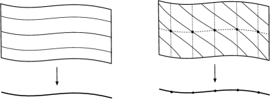
Figure 1. The integral lattice and the affine lattice

6.3 Remark.

In this section, given any integral-integral affine manifold $B$, we constructed its affine lattice $\Lambda^{\operatorname{aff}}\subset TB$, and we viewed it as a section of the Lie torus bundle $TB/\Lambda$. In §4, we started with a prequantized Lagrangian torus fibration $L\to M\to B$, and we obtained from it an integral-integral structure on $B$. When $B$ is obtained in this way, we can identify the Lie torus bundle $TB/\Lambda$ as the dual torus bundle associated to $M\to B$, and we can construct its section $\Lambda^{\operatorname{aff}}$ directly from the prequantization. For details, see Section 9.   $\diamond$

7. Local torus actions

A Lagrangian torus fibration $M\to B$ is not quite a principal torus bundle: its fibres come with free and transitive torus actions, but there is no one single torus that acts on all of these fibres. Instead, the tori that act on these fibres assemble into a Lie torus bundle. This Lie torus bundle comes with local trivializations, which give torus actions on neighbourhoods of fibres of $M$, and these fit together into a local torus action. In this section we provide details and we generalize some standard results on global torus actions to local torus actions.

Local torus actions

Fix a Lie torus $T$, namely, a Lie group isomorphic to $(S^{1})^{n}$.

7.1 Definition.

A $T$-atlas on a manifold $M$ is a set of open subsets of $M$ that cover $M$ and are equipped with $T$-actions, satisfying the following compatibility condition: Given two such open subsets $U$ and $V$, the intersection $U\cap V$ is invariant under both actions, and on each of its connected components, the actions differ by an automorphism of $T$. Two $T$-atlases are equivalent if their union is also a $T$-atlas, namely, if their union satisfies the same compatibility condition. A local $T$-action on $M$ is an equivalence class of $T$-atlases.

7.2 Remark.

There are several different definitions of “local torus action” in the literature, none of which are exactly the same as ours; some others are in [Y] and [CG], [Gm].

7.3 Remark.

Our definition of local torus actions, and their resulting properties, naturally extend to arbitrary compact Lie groups. In this paper, we only need local torus actions that come from Lie torus bundles, as in the following example. These can also be viewed as Lie groupoid actions.

7.4 Example.

Let $p\colon N\to B$ be a Lie torus bundle (see §6) with fibres isomorphic to $T$. A local trivialization $p^{-1}(U)\cong U\times T$ induces a natural action of $T$ on $p^{-1}(U)$ by acting on the second component of $U\times T$. Because the automorphism group of the Lie torus $T$ is discrete, for any two such local trivializations, the $T$ actions on the (connected components of the) intersection of their domains differ by an automorphism of $T$. This equips $N$ with a local $T$-action.

We say that a $k$-form $\alpha\in\Omega^{k}(M)$ is invariant with respect to the local torus action if the restriction of $\alpha$ to every element of every $T$-atlas is $T$-invariant. (Because being $T$-invariant is preserved under automorphisms of $T$, it is enough to require the existence of one $T$-atlas such that restrictions of $\alpha$ to its elements are $T$-invariant.) Denote by $\Omega^{k}(M)^{T}$ the space of invariant $k$-forms on $M$.

Next, define an “averaging” map $\operatorname{av}\colon\alpha\mapsto\overline{\alpha}\colon\Omega^{k}(M)\to\Omega^{k}(M)^{T}$ as follows. In any open set $U$ in a T-atlas, it is defined by integrating over the torus:

$$\overline{\alpha}|_{U}=\int_{t\in T}t^{*}\alpha|_{U}\,d\mu$$

where $d\mu$ is normalized Haar measure on $T$. This construction agrees on overlaps between different elements of a T-atlas, since the Haar measure is invariant under $\operatorname{Aut}(T)$, and so this operation is well-defined over all of $M$. Note that $\alpha$ is invariant iff $\bar{\alpha}=\alpha$.

Invariance and averaging are compatible with the exterior derivative:

7.5 Lemma.

Let $M$ be a manifold equipped with a local $T$-action. For any $\alpha\in\Omega^{k}(M)$, we have $\overline{d\alpha}=d\bar{\alpha}$. Thus, if $\alpha$ is invariant, then $d\alpha$ is invariant, and if $\alpha$ is closed, then $\bar{\alpha}$ is closed.

Proof.

The argument is similar to the known argument for a global $T$ action; we include it here for completeness.

In a local coordinate chart contained in an element of a $T$-atlas, write $t^{*}\alpha=\sum_{I}a_{I}(x,t)dx_{I}$. Then

$$\overline{\alpha}=\sum_{I}\Big{(}\int_{T}a_{I}(x,t)dt\Big{)}dx_{I},$$

where the integral is with respect to the normalized Haar measure on $T$. Similarly,

$$\overline{d\alpha}=\sum_{I,j}\Big{(}\int_{T}\frac{\partial a_{I}}{\partial x_{j}}(x,t)dt\Big{)}dx_{j}\wedge dx_{I}.$$

So it suffices to show that, for each $I$ and $j$,

$$\int_{T}\frac{\partial a_{I}}{\partial x_{j}}(x,t)\,dt=\frac{\partial}{\partial x_{j}}\left(\int_{T}a_{I}(x,t)\,dt\right).$$

This, in turn, follows from Theorem 9.42 in [R], differentiation under the integral sign, which requires only continuity of $\frac{\partial a_{I}}{\partial x_{j}}$. Since each point has a neighbourhood where $\overline{d\alpha}=d\overline{\alpha}$, we are done.

For the second claim, recall that $\beta$ is invariant if and only if $\overline{\beta}=\beta$, and note that $\overline{0}=0$. ∎

The key fact we will need about local torus actions is that, when the manifold is compact, any cohomology class has an invariant representative. We prove this in Theorem 7.6. We expect this fact to remain true for non-compact manifolds; it should follow from the fact that the subspace of exact forms is closed (say, in the $C^{\infty}$ topology) in the space of all differential forms. For a global action on a non-compact manifold, an easier proof is given in [O, §9].

7.6 Theorem.

Let $M$ be a compact manifold equipped with a local $T$ action. Then, for each closed $k$-form $\alpha$, its average $\overline{\alpha}$ is closed, and the cohomology classes of $\overline{\alpha}$ and $\alpha$ are equal in $H^{k}(M)$. In particular, any cohomology class in $H^{k}(M)$ has a representative in $\Omega^{k}(M)^{T}$.

Proof.

Let $M$ be a compact manifold equipped with a local $T$ action. Denote $H^{k}(\Omega^{\bullet}(M)^{T},d)$ by $H^{k}_{\operatorname{inv}}(M)$. Since the condition of invariance is preserved by the exterior derivative, i.e., $d\bigl{(}\Omega^{k}(M)^{T}\bigr{)}\subseteq\Omega^{k+1}(M)^{T}$, the inclusion map $\iota\colon\Omega^{k}(M)^{T}\hookrightarrow\Omega^{k}(M)$ induces a map on cohomology,

$$\iota_{*}\colon H^{k}_{\operatorname{inv}}(M)\to H_{{\operatorname{dR}}}^{k}(M).$$

Since the averaging map $\operatorname{av}\colon\alpha\mapsto\overline{\alpha}$ also commutes with $d$, it also induces a map on cohomology

$$\operatorname{av}_{*}\colon H_{{\operatorname{dR}}}^{k}(M)\to H^{k}_{\operatorname{inv}}(M).$$

Note that the composition $\operatorname{av}_{*}\iota_{*}$ is the identity map on $H^{k}_{\operatorname{inv}}(M).$

Fix a finite $T$ atlas $\{U_{1},\ldots,U_{m}\}$ on $M$. We will prove by induction on $\ell$ that the map

(7.7) $${}\iota_{*}\colon H_{\operatorname{inv}}^{k}\left(\cup_{i=1}^{\ell}U_{i}\right)\to H^{k}_{\operatorname{dR}}\left(\cup_{i=1}^{\ell}U_{i};\mathbb{R}\right)$$

is an isomorphism for all $k$.

The case $\ell=1$ follows from the fact that, because $T$ is a compact connected Lie group and $U_{1}$ is a $T$ manifold, $H^{k}_{{\operatorname{dR}}}(U_{1};\mathbb{R})=H^{k}\left(\Omega^{\bullet}(U_{1})^{T},d\right)$; see [O, §9].

Next, fixing $1\leq\ell<m$, suppose that (7.7) is an isomorphism for all $k$, and we would like to prove that

$$\iota_{*}\colon H_{\operatorname{inv}}^{k}\left(\cup_{i=1}^{\ell+1}U_{i}\right)\to H^{k}_{\operatorname{dR}}\left(\cup_{i=1}^{\ell+1}U_{i};\mathbb{R}\right)$$

is an isomorphism for all $k$.

Consider the following commutative diagram of Mayer–Vietoris long exact sequences

Since each $U_{j}$ is $T$-invariant, so is the intersection $\bigl{(}\cup_{i=1}^{\ell}U_{i}\bigr{)}\cap U_{\ell+1}$. Because we have an actual $T$ action on this intersection,

(7.8) $${}\iota_{*}\colon H_{\operatorname{inv}}^{k}\Bigl{(}\bigl{(}\cup_{i=1}^{\ell}U_{i}\bigr{)}\cap U_{\ell+1}\Bigr{)}\to H^{k}_{{\operatorname{dR}}}\Bigl{(}\bigl{(}\cup_{i=1}^{\ell}U_{i}\bigr{)}\cap U_{\ell+1}\Bigr{)}$$

is an isomorphism, giving the right-hand vertical arrow in the above diagram. The middle vertical arrow is the map $\iota_{*}\oplus\iota_{*}$; the first $\iota_{*}$ is an isomorphism by the induction hypothesis, and the second is an isomorphism because there is a global $T$-action on $U_{\ell+1}$. Since these maps are isomorphisms for all $k$, the Five Lemma implies that the left-hand vertical map

$$\iota_{*}\colon H_{\operatorname{inv}}^{k}\Bigl{(}\bigl{(}\cup_{i=1}^{\ell}U_{i}\bigr{)}\cup U_{\ell+1}\Bigr{)}\to H_{{\operatorname{dR}}}^{k}\Bigl{(}\bigl{(}\cup_{i=1}^{\ell}U_{i}\bigr{)}\cup U_{\ell+1}\Bigr{)}$$

is also an isomorphism.

This completes the induction, and proves $\iota_{*}\colon H^{k}_{\operatorname{inv}}(M)\to H_{{\operatorname{dR}}}^{k}(M)$ is an isomorphism.

Finally, since $\operatorname{av}_{*}$ is a left inverse of $\iota_{*}$ and $\iota_{*}$ is an isomorphism, $\operatorname{av}_{*}$ is the inverse of $\iota_{*}$. ∎

8. Proof of “Downstairs Theorem”

The purpose of this section is to prove Theorem 3.1, whose statement we now recall:

Theorem (3.1, restated).

Let $B$ be a compact integral-integral affine manifold. Then the volume of $B$ is equal to the number of integral points in $B$:

$$\operatorname{vol}(B)=\lvert B_{\mathbb{Z}}\rvert.$$

Let $B$ be an integral-integral affine manifold. After passing to a double covering, if necessary, we fix an orientation of $B$. (Note that the double covering inherits an integral-integral affine structure, and that if Theorem 3.1 holds for the double covering, then it holds for the original $B$.)

Let $\Lambda\subset TB$ be the integral lattice. Then $M^{\vee}:=TB/\Lambda$ is a Lie torus bundle over $B$ (see Proposition 6.1); let $\pi^{\vee}\colon M^{\vee}\to B$ denote the projection. Let $Z_{0}\subset M^{\vee}$ be induced from the zero section of $TB$.

Given adapted coordinates $x_{1},\ldots,x_{n},y_{1},\ldots,y_{n}$ on $TB$ as in Proposition 6.1, taking $y_{j}$ mod 1 gives what we call “adapted coordinates” on $M^{\vee}$.

8.1 Lemma.

There exists a unique closed $n$-form $dy^{n}$ on $M^{\vee}$ such that, in any adapted coordinates on $M^{\vee}$ as above, we have $dy^{n}=dy_{1}\wedge\ldots\wedge dy_{n}$.

Proof.

Given two different sets $(x_{1},\ldots,x_{n},y_{1},\ldots,y_{n})$ and $(x_{1}^{\prime},\ldots,x_{n}^{\prime},y_{1}^{\prime},\ldots,y_{n}^{\prime})$ of coordinates on $M^{\vee}$ as above, the $x$ and $x^{\prime}$ coordinates will locally differ by $x^{\prime}=Ax+b$ with $A\in\operatorname{GL}_{n}(\mathbb{Z})$ and $b\in\mathbb{R}^{n}$, and the $y$ coordinates will locally differ by $y^{\prime}=Ay$ with the same $A\in\operatorname{GL}_{n}(\mathbb{Z})$. Because the $x$ and $x^{\prime}$ coordinates are oriented, the determinant of $A$ is positive, hence it is $1$. It follows that $dy_{1}\wedge\ldots\wedge dy_{n}=dy_{1}^{\prime}\wedge\ldots\wedge dy_{n}^{\prime}$. ∎

We orient $M^{\vee}$ such that every set of coordinates $x_{1},\ldots,x_{n},y_{1},\ldots,y_{n}$ as above is oriented.

8.2 Proposition.

The cohomology class $[dy^{n}]$ is the Poincaré dual of the submanifold $Z_{0}$.

Proof.

We need to show that, given any closed $n$-form $\alpha$ on $M^{\vee}$,

(8.3) $${}\int_{Z_{0}}\alpha=\int_{M^{\vee}}\alpha\wedge dy^{n}.$$

As in Example 7.4, the Lie torus bundle $M^{\vee}$ has a local $T$-action, which in coordinates as above is given by translations on the $y_{j}$ (mod 1) coordinates. By Theorem 7.6, we may assume that $\alpha$ is invariant under this local torus action.

Let $\{U_{k}\}$ be an open cover of $B$ such that on each $U_{k}$ there exists an integral affine chart, and let $\{\rho_{k}\}$ be a partition of unity subordinate to this cover. Let $\alpha_{k}:=(\pi^{\vee})^{*}\rho_{k}\cdot\alpha$; then

$$\int_{Z_{0}}\alpha=\sum_{k}\int_{Z_{0}}\alpha_{k}\qquad\text{ and }\qquad\int_{M^{\vee}}\alpha\wedge dy^{n}=\sum_{k}\int_{M^{\vee}}\alpha_{k}\wedge dy^{n}.$$

The $n$-forms $\alpha_{k}$ are still invariant (they might no longer be closed, but this will end up not creating a problem), so it remains to show that (8.3) holds when $\alpha$ is replaced by the invariant $n$-form $\alpha_{k}$.

In adapted coordinates over $U_{k}$, the invariant $n$-form $\alpha_{k}$ is a sum of terms of the form $c(x)\,dx_{i_{1}}\wedge\ldots\wedge dx_{i_{r}}\wedge dy_{j_{1}}\wedge\ldots\wedge dy_{j_{s}}$ with $r+s=n$. Taking its wedge with $dy^{n}$, all terms with $s>0$ vanish, and we obtain

$$\alpha_{k}\wedge dy^{n}=c_{k}(x)\,dx_{1}\wedge\ldots\wedge dx_{n}\wedge dy_{1}\wedge\ldots\wedge dy_{n}$$

for some smooth $c_{k}$ depending only on $x$.

In these same coordinates, the submanifold $Z_{0}$ is parametrized by the map

$$s_{0}\colon U_{k}\to Z_{0}\quad,\quad x\mapsto(x,[0]),$$

and the pullback of $\alpha_{k}$ by this map is given by

$$s_{0}^{*}\alpha_{k}=c_{k}(x)\,dx_{1}\wedge\cdots\wedge dx_{n}$$

with the same coefficient $c_{k}(x)$. So

$$\int_{M^{\vee}}\alpha_{k}\wedge dy^{n} =\int_{U_{k}\times(\mathbb{R}/\mathbb{Z})^{n}}c_{k}(x)\,dx_{1}\wedge\ldots\wedge dx_{n}\wedge dy_{1}\wedge\cdots\wedge dy_{n}$$

$$=\left(\int_{U_{k}}c_{k}(x)\,dx_{1}\wedge\cdots\wedge dx_{n}\right)\left(\int_{(\mathbb{R}/\mathbb{Z})^{n}}dy_{1}\wedge\cdots\wedge dy_{n}\right)$$

$$=\int_{U_{k}}c_{k}(x)\,dx_{1}\wedge\cdots\wedge dx_{n}$$

$$=\int_{Z_{0}}\alpha_{k},$$

as required. ∎

Finally, recall from Section 6 that $M^{\vee}$ comes with a section $D\subset M^{\vee}$ that in local coordinates as above is given by $D=\{(x,[-x])\}$. The orientation of $B$ induces orientations of $Z_{0}$ and of $D$, and as noted in Section 6, $D$ intersects $Z_{0}$ above $B_{\mathbb{Z}}$, so $\lvert D\cap Z_{0}\rvert=\lvert B_{\mathbb{Z}}\rvert$. The intersection number of $Z_{0}$ with $D$ is then $(-1)^{n}\lvert D\cap Z_{0}\rvert$.

The pullback of $dy^{n}$ by the map $s(x)=(x,[-x])$ that parametrizes $D$ is $(-1)^{n}dx_{1}\wedge\ldots\wedge dx_{n}$. We then have

$$\lvert B_{\mathbb{Z}}\rvert=(-1)^{n}\big{(}[D]\cup[Z_{0}]\big{)}=(-1)^{n}\int_{D}\operatorname{PD}(Z_{0})=(-1)^{n}\int_{D}dy^{n}\\ =\int_{B}(-1)^{n}s^{*}dy^{n}=\int_{B}dx_{1}\wedge\cdots\wedge dx_{n}=\operatorname{vol}(B).$$

This completes the proof of Theorem 3.1.

9. Dual torus fibrations

In this section we collect some material that we don’t strictly need for our proof, and that is well-known, but that may help clarify the geometric context of the structures that we have been considering.

In the proof of our Downstairs Theorem in §8, a key ingredient was a section of $TB/\Lambda$, constructed from the integral-integral affine structure, whose intersections with the zero section are the integer points of $B$. From the “upstairs” viewpoint, this section is determined by the prequantization line bundle, and its intersections with the zero-section are the Bohr–Sommerfeld points. In this section we briefly explain how to define the section directly from the line bundle, and how it corresponds with the construction via integral-integral affine structures.

A flat circle bundle is a principal circle bundle equipped with a flat connection. For any manifold $N$, there is a natural bijection between the set of equivalence classes of flat circle bundles over $N$ and the set of isomorphism classes of complex Hermitian line bundles over $N$ equipped with flat Hermitian connections.

For any smooth torus $N$, we denote by $N^{\vee}$ the set of equivalence classes of flat circle bundles over $N$. This set is naturally a Lie torus, e.g., by using the holonomy to identify $N^{\vee}$ with $\operatorname{Hom}(\pi_{1}(N),S^{1})$ (for any choice of basepoint). We will call $N^{\vee}$ the dual torus to $N$. Any diffeomorphism $N_{1}\cong N_{2}$ naturally induces an isomorphism of Lie tori $N_{1}^{\vee}\cong N_{2}^{\vee}$.

For any torus $T$ with Lie algebra ${\mathfrak{t}}$, the exponential map ${\mathfrak{t}}\to T$ is a group homomorphism, the integral lattice ${\mathfrak{t}}_{\mathbb{Z}}$ is its kernel, and we obtain identifications $T={\mathfrak{t}}/{\mathfrak{t}}_{Z}$ and $\pi_{1}(T)={\mathfrak{t}}_{\mathbb{Z}}$. The dual lattice $\operatorname{Hom}({\mathfrak{t}}_{\mathbb{Z}},\mathbb{Z})$ embeds in ${\mathfrak{t}}^{*}=\operatorname{Hom}({\mathfrak{t}},\mathbb{R})$ through tensoring with $\mathbb{R}$, yielding the weight lattice ${\mathfrak{t}}_{\mathbb{Z}}^{*}\subset{\mathfrak{t}}^{*}$. Writing elements of $S^{1}$ as $e^{2\pi it}$, we obtain an identification $S^{1}=\mathbb{R}/\mathbb{Z}$, which yields ${\mathfrak{t}}_{\mathbb{Z}}=\operatorname{Hom}(S^{1},T)$ and ${\mathfrak{t}}_{\mathbb{Z}}^{*}=\operatorname{Hom}(T,S^{1})$.

With these identifications, $T^{\vee}=\operatorname{Hom}(\pi_{1}(T),S^{1})={\mathfrak{t}}^{*}/{\mathfrak{t}}_{\mathbb{Z}}^{*}$. For any $T$-torsor $N$, the natural identification of $\pi_{1}(N)$ with $\pi_{1}(T)$ yields $N^{\vee}=T^{\vee}={\mathfrak{t}}^{*}/{\mathfrak{t}}_{\mathbb{Z}}^{*}$.

For the standard torus $\mathbb{T}^{n}=(S^{1})^{n}$, and with the standard identification $\mathbb{R}^{n}=(\mathbb{R}^{n})^{*}$, we obtain the identifications $(\mathbb{T}^{n})^{\vee}=\mathbb{R}^{n}/\mathbb{Z}^{n}=\mathbb{T}^{n}$. In this identification, the element $(a_{1},\ldots,a_{n})$ of $\mathbb{T}^{n}$ on the right hand side corresponds to the element of $(\mathbb{T}^{n})^{\vee}$ on the left hand side that is represented by a flat connection whose holonomony along each loop $\gamma_{j}$ is $a_{j}$, where $\gamma_{j}$ is the loop in the $t_{j}$ coordinate.

Let $\pi\colon M\to B$ be a (smooth) torus fibration. As a set, the dual torus fibration $M^{\vee}\to B$ consists of the disjoint union of the dual tori; namely, for each $x\in B$, the fibre $(M^{\vee})_{x}$ is the set of equivalence classes of flat circle bundles over the fibre $M_{x}$. The local trivializations $M|_{U}\cong U\times\mathbb{T}^{n}$ induce a manifold structure on $M^{\vee}$ and local trivializations $M^{\vee}|_{U}\cong U\times\mathbb{T}^{n}$, making $M^{\vee}$ into a Lie torus fibration.

Given a Lagrangian torus fibration $M\to B$ and a prequantization line bundle $L\to M$, the restriction of $L$ to each Lagrangian torus fibre $M_{x}$ is flat, thus it determines an element of the corresponding dual torus, which is trivial if and only if $M_{x}$ is a Bohr–Sommerfeld fibre (by definition). Thus, $L$ induces a section

$$s_{L}\colon B\to M^{\vee}$$

of the dual torus bundle $M^{\vee}$, which intersects the zero section exactly above the Bohr–Sommerfeld points. Up to sign, this section coincides with the affine lattice that we introduced in Section 6, in a sense that we will now spell out.

9.1 Proposition.

1. Given a Lagrangian torus fibration $M\to B$, the dual fibration $M^{\vee}$ is naturally isomorphic as a Lie torus bundle to $TB/\Lambda$, where $\Lambda$ is the integral lattice arising from the induced integral affine structure on $B$ (as in §6).

2. Let $L\to M\to B$ be a prequantized Lagrangian torus fibration, and let $\Lambda^{\text{aff}}$ be the affine lattice arising from the induced integral-integral affine structure on $B$ (as in §6). Then the isomorphism $M^{\vee}\cong TB/\Lambda$ of part (1) identifies $s_{L}$ with $-\Lambda^{\text{aff}}$ viewed as a section of $TB/\Lambda$.

Sketch of proof.

Part (1) is obtained from the proof of the Arnol’d–Liouville theorem. Namely, by taking time-1 Hamiltonian flows of collective functions (pullbacks to $M$ of smooth functions on $B$), we obtain for each $x\in B$ an action of $T_{x}^{*}B$ on the fibre $M_{x}$. This action has stabilizer $\Lambda^{*}_{x}$, so makes $M_{x}$ into a $T_{x}^{*}B/\Lambda^{*}_{x}$-torsor. Therefore we can identify $M_{x}^{\vee}$ with the torus dual to $T_{x}^{*}B/\Lambda^{*}_{x}$, namely, with $T_{x}B/\Lambda_{x}$.

Part (2) then follows from the coordinate expression of $s_{L}$ in an enhanced Arnol’d–Liouville chart. Here are some details: By “enhanced Arnol’d–Liouville” (Theorem 4.8), we may assume that $L=\Omega\times\mathbb{T}^{n}\times\mathbb{C}$, with coordinates $(x_{1},\ldots,x_{n},t_{1},\ldots,t_{n},z)$ with $t_{j}$ taken mod $1$. In particular, we identify $M=\Omega\times\mathbb{T}^{n}$ and $B=\Omega$. From these identifications, we obtain $M^{\vee}=\Omega\times(\mathbb{T}^{n})^{\vee}$ and $TB=\Omega\times\mathbb{R}^{n}$ and $\Lambda=\Omega\times\mathbb{Z}^{n}$, so $TB/\Lambda=\Omega\times\mathbb{T}^{n}$. Composing with our identification $(\mathbb{T}^{n})^{\vee}=\mathbb{T}^{n}$, we obtain the identification $TB/\Lambda=M^{\vee}$ of Part 1. Finally, by Lemma 4.7, the holonomy along $\gamma_{j}$ of the connection in the enhanced Arnol’d–Liouville chart is $e^{2\pi ix_{j}}$; using our identification $(\mathbb{T}^{n})^{\vee}=\mathbb{T}^{n}$, we obtain $s_{L}(x_{1},\ldots,x_{n})=(x_{1},\ldots,x_{n},e^{2\pi ix_{1}},\ldots,e^{2\pi ix_{n}})$, also written as $(x,[x])$, which is the negative of the expression in coordinates for the section $\Lambda^{\operatorname{aff}}$ (6.2). ∎

10. Comments on the literature

The results and ideas that we present in this paper are in principle known to experts. In particular, our Upstairs Theorem follows from a more general theorem of Fujita, Furuta, and Yoshida, and appears as Corollary 6.12 in their paper [FFY]. They, in turn, attribute this result to Andersen’s paper [And]; however, Andersen’s paper does not explicitly contain this result. Corollary 4.1 of Andersen’s paper [And] is similar, and its proof contains ingredients that are similar to ours, but this proof lacks detail.

Specifically, Andersen’s Corollary 4.1 should follow from the proof of his Theorem 4.1. In the proof of his Theorem 4.1, Andersen describes an $n$-form $\alpha$ on a torus bundle (which is the same as the $n$-form $dy^{n}$ on $M^{\vee}$ in our Lemma 8.1), and writes: “It is clear that $\alpha$ is the Poincaré dual of the zero section”. To us, this was not “clear;” this result is our Proposition 8.2, whose proof relies on our nontrivial Theorem 7.6.

Andersen [And] also works with the half-form correction and we don’t (yet), but this difference should be minor. Finally, Andersen works with so-called mixed polarizations, of which our Lagrangian fibrations are a very special case; it would be interesting to extend our work to Andersen’s more general setup.

Our proof of Theorem 3.1 is inspired by Gross’s “Mirror Riemann–Roch conjecture” [Gr, Conjecture 4.9]. In the presence of a (special) Lagrangian torus fibration and a (“permissible”) dual fibration, this conjecture expresses the Euler characteristic of a holomorphic line bundle over one of the fibrations as an intersection number of sections of the other fibration, up to sign.

Similar ideas also appear in Tyurin’s paper [T]. Tyurin works with a singular Lagrangian fibration of a compact Käler manifold $M$, with a prequantization line bundle $M\to L$. He refers to the question on whether the dimension of the space of holomorphic sections equals the number of Bohr–Sommerfeld fibres for $L^{\otimes k}$ as the “numerical quantization problem” [T, p. 6]. (About this dimension, see our discussion in Section 2 under “Riemann–Roch numbers”.) He sketches a general argument for attacking this problem by realizing the Bohr–Sommerfeld set as the intersection of two sections of a dual fibration. (The proof of the “Downstairs Theorem” in our Section 8 uses a similar idea.) Tyurin applies this general method to the cases of elliptic curves (Prop 1.4 and Cor 1.1), K3 surfaces (Theorem 2.2), and “conditionally” to Calabi–Yau 3-folds (Prop 3.2 and Cor 3.1; see the first paragraph of §3 for a discussion of the “conditionality”). He acknowledges that “these constructions have been developed and used by a number of physicists and mathematicians.”

Tyurin works with Kähler manifolds, and allows the polarizations to have nodal (“focus-focus”) singularities (see (2.54) on p. 30). In our setting, we do not allow singularities in our polarizations; on the other hand, integrability of almost complex structures is not assumed. In particular, our proof applies to the Kodaira–Thurston manifold, but the argument in [T] doesn’t. It would be interesting to extend our work to allow focus-focus singularities.

References

- [And] Jørgen E. Andersen, Geometric quantization of symplectic manifolds with respect to reducible non-negative polarizations, Commun. Math. Phys. 183, 401–421 (1997).
- [Arn2] V.I. Arnol’d, Mathematical methods of classical mechanics, Second Edition, Springer, New York, 1989.
- [CG] Cheeger and Gromov, Collapsing Riemannian manifolds while keeping their curvature bounded I, J. Diff Geom. 23 (1986), 309–346.
- [D1] J. J. Duistermaat, The heat kernel Lefschetz fixed point formula for the spin-c Dirac operator, Birkhäuser, Boston, 2011.
- [D2] J. J. Duistermaat, On Global Action-Angle Coordinates, Comm. Pure Appl. Math. 33 (1980), no. 6, 687–706
- [FM] Rui Loja Fernandes and Maarten Mol, Kähler metrics and toric Lagrangian fibrations, arXiv:2401.02910 [math.DG]
- [FFY] Hajime Fujita, Mikio Furuta, and Takahiko Yoshida, Torus fibrations and localization of index I – polarization and acyclic fibrations, J. Math. Sci. Univ. Tokyo 17 (2010), 1–26.
- [GGK] Viktor Ginzburg, Victor Guillemin, and Yael Karshon Moment Maps, Cobordisms, and Hamiltonian Group Actions, Mathematical Surveys and Monographs, 98, American Mathematical Society, Providence, RI, 2002.
- [Go] William M. Goldman, Geometric structures on manifolds, Graduate Studies in Mathematics 227, Amer. Math. Soc., 2022.
- [Gm] Gromov, Volume and bounded cohomology, Publ. IHES 56 (1983), 213–307
- [Gr] Mark Gross, Special Lagrangian Fibrations I: Topology. Integrable systems and algebraic geometry (Kobe/Kyoto, 1997), 156-193, World Sci. Publ., River Edge, NJ, 1998.
- [GS] V. Guillemin and S. Sternberg, The Gel’fand–Cetlin system and quantization of the complex flag manifolds, J. Funct. Anal. 52 (1983), no. 1, 106–128
- [H] M. D. Hamilton, Classical and quantum monodromy via action-angle variables, Journal of Geometry and Physics, 115 (May 2017), 37–44
- [HM] M. D. Hamilton and Zoe McIntyre, Quantum monodromy in the Kodaira-Thurston manifold, in progress.
- [K] B. Kostant, Quantization and unitary representations. I. Prequantization, Lectures in modern analysis and applications, III, Lecture Notes in Mathematics, 170, pp. 87–208
- [KSW] Yael Karshon, Shlomo Sternberg, and Jonathan Weitsman, Exact Euler-Maclaurin formulas for simple polytopes, Adv. Appl. Math. 39 (2007), 1–50.
- [MM] L. Markus and K.R. Meyer, Generic Hamiltonian systems are neither integrable nor ergodic, Mem. A.M.S. 144, 1974.
- [Mo] Maarten Mol, On the classification of multiplicity-free Hamiltonian actions by regular proper symplectic groupoids, arXiv:2401:00570 [math.SG]
- [O] Arkadi L. Onishchik, Topology of transitive transformation groups, Barth Verlagsgesellschaft, Barth 1994
- [R] W. Rudin, Principles of Mathematical Analysis, third edition, McGraw-Hill, 1976
- [Se] Daniele Sepe, Topological classification of Lagrangian fibrations, Journal of Geometry and Physics 60, 341–351 (2010)
- [Sn] Jedrzej Śniatycki, On cohomology groups appearing in geometric quantization, in: Lecture Notes in Math. 570, Springer-Verlag, Berlin, 1977, pp. 46–66.
- [T] Andrei Tyurin, Geometric quantization and mirror symmetry, arXiv:math/9902027v1
- [W] N.M.J. Woodhouse, Geometric Quantization, 2nd edition, Clarendon Press, Oxford, 1991
- [Y] Takahiko Yoshida, Local torus actions modeled on the standard representation, Advances in Mathematics, 227 5 (Aug 2011), 1914–1955.