Constant Workspace Algorithms for Computing Relative Hulls in the Plane

Abstract

The constant workspace algorithms use a constant number of words in addition to the read-only input to the algorithm stored in an array. In this paper, we devise algorithms to efficiently compute relative hulls in the plane using a constant workspace. Specifically, we devise algorithms for the following three problems:
(i) Given two simple polygons $P$ and $Q$ with $P\subseteq Q$, compute a simple polygon $P^{\prime}$ with a perimeter of minimum length such that $P\subseteq P^{\prime}\subseteq Q$.
(ii) Given two simple polygons $P$ and $Q$ such that $Q$ does not intersect the interior of $P$ but it does intersects with the interior of the convex hull of $P$, compute a weakly simple polygon $P^{\prime}$ contained in the convex hull of $P$ such that the perimeter of $P^{\prime}$ is of minimum length.
(iii) Given a set $S$ of points located in a simple polygon $P$, compute a weakly simple polygon $P^{\prime}\subseteq P$ with a perimeter of minimum length such that $P^{\prime}$ contains all the points in $S$.
To our knowledge, no prior works devised algorithms to compute relative hulls using a constant workspace and this work is the first such attempt.

1 Introduction

A polygon is the image of a piecewise linear closed curve. A simple polygon is the image of a piecewise linear simple closed curve such that any two successive line segments along its boundary intersect at their endpoints. A polygon $P$ with at least three sides is called a weakly simple polygon whenever each of the vertices of $P$ can be perturbed by at most $\epsilon$ to obtain a simple polygon for every real number $\epsilon>0$. A simple polygon $P$ in $\mathbb{R}^{2}$ is convex whenever the line segment $pq$ is contained in $P$ for every two points $p,q\in P$. Computing the convex hull in the plane is a fundamental problem in computational geometry. Specifically, the following two problems are of interest: (i) Given a set $S$ of $n$ points in the plane, finding a convex (simple) polygon $CH(S)$ with perimeter of minimum length so that $CH(S)$ contains all the points in $S$. (ii) Given a simple polygon $P$ in the plane defined with $n$ vertices, finding a convex (simple) polygon $CH(P)$ with perimeter of minimum length that contains $P$. It is well known that both $CH(S)$ and $CH(P)$ are unique. The famous algorithms for the first problem include Jarvis’s march (a specialization of Chand and Kapur’s gift wrapping), Graham’s scan, Quickhull algorithm, Shamos’s merge algorithm, Preparata-Hong’s merge algorithm, incremental and randomized incremental algorithms. Many of these algorithms are detailed in popular textbooks on computational geometry, Preparata and Shamos [21] and de Berg et al. [15]. The worst-case lower bound on the time complexity of the first problem is known to be $\Omega(n\lg{h})$. Several optimal algorithms that take $\Theta(n\lg{h})$ worst-case time are known; for example, algorithms by Kirkpatrick and Seidel [18] and Chan [13]. For the second problem, several algorithms with $O(n)$ time complexity, where $n$ is the number of vertices of $P$, are known; the one by Lee is presented in [21].

The relative hull, also known as the geodesic convex hull, has received increasing attention in computational geometry, which appears in a variety of applications in robotics, industrial manufacturing, and geographical information systems. The relative hulls and their related structures based on geodesic metrics have been used to approximate curves and surfaces in digital geometry. The following two specific problems on relative hulls are famous: (i) Given two simple polygons $P$ and $Q$ with $P\subset Q$, computing a simple polygon, known as the relative hull of $P$ with respect to $Q$, denoted by $RH(P|Q)$, with a perimeter of minimum length such that $P\subseteq RH(P|Q)\subseteq Q$. (ii) Given a set $S$ of points located in a simple polygon $Q$, computing a weakly simple polygon, known as the relative hull of $S$ with respect to $Q$, denoted by $RH(S|Q)$, with a perimeter of minimum length such that $RH(S|Q)$ contains all the points in $S$ and is contained in $Q$. Toussaint [23] devises algorithms for both of these problems. The main idea of their algorithm for the first problem is as follows. For every edge $e$ of $CH(P)$, if $e$ does not intersect any edge of $Q$, then $e$ is included in the relative hull. Otherwise, their algorithm identifies a simple polygon $P^{\prime}$ formed by the pocket defined by $e$ sans the exterior of $Q$, and all the edges of the geodesic shortest path between the endpoints of $e$ in $P^{\prime}$ are included in the relative hull. More details of this algorithm are given in Section 2. For the second problem, the algorithm given in [23] computes a weakly simple polygon $Q^{\prime}$ and then transforms that polygon into a simple polygon $Q^{\prime\prime}$ with a perimeter of minimum length. The polygon $Q^{\prime}$ is computed by triangulating the polygon $Q$, finding convex hulls of points of $S$ lying in each triangle of that triangulation, and using the dual-tree of that triangulation to connect specific points on the boundaries of some of these hulls with geodesic shortest paths. This algorithm is further detailed in Section 4. The polygon $Q^{\prime\prime}$ is obtained by finding a geodesic shortest path between two special points such that this path is a simple cycle located in $Q\backslash Q^{\prime}$.

In this paper, we consider three problems on relative hulls and devise algorithms to compute them using a constant workspace. The workspace of an algorithm is the additional space, excluding both the input and output space complexities, required to execute that algorithm. Traditionally, workspace complexity has been playing only second fiddle to time complexity; however, due to the limited space on chips, algorithms need to use space efficiently, for example, in embedded systems. For such reasons, algorithms using a small footprint are desired. The following are the three computation models that are popular in designing algorithms focusing on workspace efficiency: algorithms that work using a constant workspace, in-place algorithms, and algorithms that trade-off between time and workspace. In constant workspace algorithms, input is read-only, output is not stored but streamed, and these algorithms use an $O(1)$ workspace. The following are the well-known constant workspace algorithms: shortest paths in trees and simple polygons by Asano et al. [5], triangulating a planar point set and trapezoidalization of a simple polygon by Asano et al. [4], and separating common tangents of two polygons by Abrahamsen [1]. In the constant workspace model, Reingold [22] devised an algorithm to determine whether a path exists between any two given nodes in an undirected graph, settling a significant open problem. In-place algorithms also use $O(1)$ workspace; however, the input array is not read-only. That is, at any instant during the algorithm’s execution, the input array can contain any permutation of elements of the initial input array. Strictly speaking, these algorithms use $O(n)$ workspace, where $n$ is the input size. Here are some of the notable in-place algorithms from the literature: computing convex hulls in the plane by Bronnimann et al. [12] and Bronnimann et al. [11]. For algorithms that provide trade-off between time and workspace, $s$ is given as an input parameter, saying the worst-case upper bound on the workspace is $O(s)$. The time complexity of such algorithms is expressed as a function of $n$ and $s$, making it viable to provide an algorithmic scheme to achieve a trade-off between workspace complexity and time complexity, a lower asymptotic worst-case time complexity as $s$ grows and larger asymptotic worst-case time complexity as $s$ gets smaller. The notable results in this model include the algorithm by Asano et al.’s algorithm to compute all-nearest-larger-neighbors problems [3], Darwish and Elmasry’s planar convex hull algorithm [14], Asano et al.’s algorithm for computing the shortest path in a simple polygon [3], Peled’s algorithm for computing the shortest path in a simple polygon [16], Aronov et al.’s algorithm for triangulating a simple polygon [2], and algorithms for triangulation of points by Korman et al. [20] and Banyassady et al. [9], an algorithm for computing the $k$-visibility region of a point in a simple polygon by Bahoo et al. [6], and Banyassady et al.’s algorithm for computing the Euclidean minimum spanning tree [7]. Barba et al. [10] devises a framework that trades-off between time and workspace for applications that use the stack data structure. (A variation of this model considers $O(s\lg{n})$ number of bits as the workspace.) Note that when $s$ is $1$, these algorithms are essentially constant workspace or in-place algorithms, depending on whether the input array is read-only or has a permutation of input objects. A detailed survey of these models and famous algorithms in these models can be found in [8]. As mentioned earlier, in this paper, we devise algorithms for computing relative hulls in the plane using a constant workspace.

The convex hull of a set $S$ of points in the plane is denoted by $CH(S)$. The convex hull of a simple polygon $P$ is the convex hull of vertices of $P$, denoted by $CH(P)$. We denote the number of vertices of any (weakly) simple polygon $P$ with $|P|$. For any simple polygon $P$, the boundary (cycle) of $P^{\prime}$ is denoted by $bd(P)$. The interior of a (weakly) simple polygon $P$ is denoted by $int(P)$. The relative interior of a (weakly) simple polygon $P$ is the region resultant from the union of $int(P)$ and the boundary of $P$. For any edge $e$ of $CH(P)$ with $e\notin P$, the pocket of $e$ is the simple polygon in $CH(P)\backslash P$ with $e$ on its boundary. And, $e$ is said to be the lid of pocket induced by $e$. Let $r^{\prime}$ and $r^{\prime\prime}$ be two rays with origin at $p$. Let $\overrightarrow{v_{1}}$ and $\overrightarrow{v_{2}}$ be the unit vectors along the rays $r^{\prime}$ and $r^{\prime\prime}$, respectively. A cone $C_{p}(r^{\prime},r^{\prime\prime})$ is the set of points defined by rays $r^{\prime}$ and $r^{\prime\prime}$ such that a point $q\in C_{p}(r^{\prime},r^{\prime\prime})$ if and only if $q$ can be expressed as a convex combination of the vectors $\overrightarrow{v_{1}}$ and $\overrightarrow{v_{2}}$ with positive coefficients. When the rays are evident from the context, we denote the cone with $C_{p}$ or $C$.

Our Contributions

Traditional algorithms for finding relative hulls proceed by designing data structures that use a workspace whose size is linear in the input complexity. Since there is no restriction on the memory, these algorithms use data structures, such as stack, queue, or a doubly-connected edge list, to save the intermediate structures such as hulls or sub-polygons. Saving information in these data structures helps to avoid re-computations. However, the workspace constraints in a constant workspace setting do not permit the liberal use of such data structures to store processed information. Hence, using a constant workspace makes the problem of computing relative hulls harder, requiring engineering a solution with special techniques devoted to constant workspace algorithms. Usually, a constant time operation using a linear workspace could take linear time when only a constant workspace is allowed, increasing the overall time complexity to quadratic in the input size and even beyond in some cases.

This paper proposes algorithms for finding relative hulls in the plane for three problems. Each of these algorithms uses a constant workspace. The first problem computes the relative hull of a simple polygon $P$, which is contained in another simple polygon $Q$. The algorithm by Toussaint [23] for this problem takes $O(|P|+|Q|)$ time while using $O(|P|+|Q|)$ workspace. Our algorithm for this problem takes $O(|P|^{2}+|Q|^{2})$ time in the worst-case while using $O(1)$ workspace. Using some of the ideas from this algorithm, we proposed an $O(|P|^{2}+|Q|^{2})$ time and $O(1)$ workspace algorithm for computing the relative hull of a simple polygon $P$ when another simple polygon $Q$ is placed such that $int(P)\cap Q=\phi$ but $int(CH(P))\cap Q\neq\phi$. We call this problem a simple polygon placed alongside another simple polygon. Toussaint [24] gave an algorithm for this problem which takes $O(|P|+|Q|)$ time and $O(|P|+|Q|)$ workspace. We modify the constant workspace algorithm given in Asano et al. [4] to compute the geodesic shortest path in a simple polygon and use this modified version to provide constant workspace algorithms for these two problems. The third problem computes the relative hull of a set $S$ of points in a simple polygon $Q$. The algorithm by Toussaint [23] for this problem takes $O(|Q|+(|S|\lg{|S|}))$ time but uses $O(|Q|+|S|)$ workspace. The constant workspace algorithm we present for this problem is more involved. As part of devising this algorithm, we engineered a solution by carefully combining constant workspace algorithms for several problems: Eulerian tour of trees, constrained Delaunay triangulation of a simple polygon, constructing the triangulation in an online fashion, computing the shortest geodesic path in a sleeve, and partially computing the hulls of points lying in each triangle of triangulation, to name a few. However, unlike the algorithm in [23], our algorithm for this problem outputs a weakly simple polygon instead of a simple polygon. Our algorithm takes $O(|Q|^{3}+|S|^{2})$ time in the worst case. In these three algorithms, at several junctures, we predominantly exploit computing instead of storing design paradigm. This paradigm is both natural and commonly used in space-constrained algorithms, wherein instead of storing information computed in a data structure, to save workspace, we re-compute those elements as and when needed. To our knowledge, the algorithms presented in this paper are the first algorithms to compute relative hulls using constant workspace.

Section 2 presents an algorithm for computing the relative hull of a simple polygon located inside another simple polygon. Section 3 gives an algorithm for computing the relative hull of simple polygon $P$ when another simple polygon is placed alongside $P$. An algorithm for computing the relative hull of a set of points located in a simple polygon is given in Section 4. Conclusions are in Section 5.

2 Relative hull of a simple polygon contained in another simple polygon

Let $P$ and $Q$ be two simple polygons such that $P\cap Q=P$ and $bd(P)\cap bd(Q)=\phi$. We assume no two vertices of $P\cup Q$ have the same $x$-coordinates or $y$-coordinates. Also, we assume that no three vertices of $P\cup Q$ are collinear. To remind the reader, the hull $RH(P|Q)$ of $P$ relative to $Q$ is a simple polygon whose boundary cycle is contained in $Q\backslash P$ and has a perimeter of minimum length. It is well-known that $RH(P|Q)$ is unique for a given $P$ and $Q$. Toussaint [23] proposed an algorithm that uses an $O(|P|+|Q|)$ space. Their algorithm takes $O(|P|+|Q|)$ time in the worst case. For this problem, Wiederhold and Reyesetal [25] proposed an algorithm that takes $O(|P|^{2}+|Q|^{2})$ time in the worst-case using $O(|P|+|Q|)$ workspace. This result mainly resolves the incorrect cases from recursive implementations given by Klette [19] while claiming to have the same time and workspace bounds as in [19].

Let $p_{1}$ be any vertex of $CH(P)$. Also, let $p_{2}$ be the vertex on the $CH(P)$ that occurs next to $p_{1}$ in traversing the $bd(CH(P))$ in the clockwise direction. Since Jarvis’s march [17] for computing the convex hull of a set of points in the plane uses $O(1)$ workspace, given $p_{1}$, by applying an iteration of Jarvis’s march, we find $p_{2}$. We note that, for every vertex $v$ of $CH(P)$, $v$ is a vertex of $RH(P|Q)$. We know the leftmost vertex of $P$ is guaranteed to be a vertex of $CH(P)$; hence it is a vertex of $RH(P|Q)$. By traversing the $bd(P)$, we find $v$, and the edges of $bd(CH(P))$ are computed starting from $v$.

For every edge $p_{1}p_{2}$ so computed, let $P^{\prime}$ be the simple polygon corresponding to the pocket defined by $p_{1}p_{2}$. When $int(P^{\prime})$ has no intersection with the $bd(Q)$, our algorithm outputs $p_{1}$ and $p_{2}$. Otherwise, further processing is needed to find a geodesic shortest path from one endpoint of $p_{1}p_{2}$ to another such that that path lies in $P^{\prime\prime}=P^{\prime}\cap Q$. We modify the algorithm given by Asano et al. [4] to compute the geodesic shortest path from $p_{1}$ to $p_{2}$ in the simple polygon $P^{\prime\prime}$.

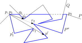
Figure 1: Illustrating $P^{\prime\prime}$ in blue colour whose boundary is made up of two polygonal chains: $p_{1},q_{1},q_{2},\ldots,p_{2}$ consisting of sections of line segment $p_{1}p_{2}$ together with sections of $bd(Q)$, and $p_{1},p_{1}^{\prime},\ldots,p_{2}$ consisting of a contiguous section of $bd(P)$. Also, illustrates extending ray $p_{1}r_{1}$ of cone $C_{p_{1}}(p_{1}r_{1},p_{1}q_{1})$ to $p^{\prime}$, and cone $C_{p_{1}}(p_{1}p^{\prime},p_{1}q_{1})$ leading to determining the next cone $C_{p_{1}}(p_{1}r_{2},p_{1}q_{1})$.

The boundary of $P^{\prime\prime}$ consists of $P\cap P^{\prime}$, the maximal sections of $p_{1}p_{2}$ that are bounding $P^{\prime}\cap Q$, and the $bd(Q)\cap P^{\prime}$. Refer to Fig. 1. Note that some of the vertices of $P^{\prime\prime}$ are incident to $p_{1}p_{2}$. Due to memory constraints, we do not precompute $P^{\prime\prime}$. Instead, based on the need, we determine the vertex of interest on the fly. Let $r$ be any vertex of $Q$ in the half-plane defined by the line induced by $p_{1}p_{2}$ that contains $P^{\prime}$. When traversing the $bd(Q)$ in the clockwise direction starting from $r$, let $q_{1}$ be the first intersection of $bd(Q)$ with $P^{\prime}$, and let $q_{2}$ be the first vertex of $bd(Q)$ that occurs in $P^{\prime}$. The $q_{1}$ can be found by finding the intersection of $p_{1}p_{2}$ with each of the edges of $Q$. Also, the vertex $q_{2}$ can be found by traversing the $bd(Q)$ in the clockwise direction starting from $q_{1}$. Specifically, we invoke the shortest path algorithm in [4] with cone $C_{p_{1}}(p_{1}q_{2},p_{1}q_{1})$.

Suppose the algorithm in [4] intends to extend the ray $pr_{1}$ of cone $C_{p}(pr_{1},pr_{2})$, where $r_{1}$ is a vertex of $P^{\prime\prime}$. Then, we determine the point of intersection $p^{\prime}$ of $pr_{1}$ with $P\cap P^{\prime}$, and the point of intersection $q^{\prime}$ of $pr_{1}$ with $bd(Q)\cap P^{\prime}$. If $p^{\prime}$ and $q^{\prime}$ exist, we determine the one among these two points closest to point $r_{1}$ along the ray $pr_{1}$. Significantly, the section of $bd(P\cap P^{\prime})$ traversed in the clockwise direction from $r_{1}$ in determining $p^{\prime}$ is not going to be traversed again in the algorithm. When the algorithm needs to find a ray’s intersection with the $bd(P\cap P^{\prime})$, we find this intersection by traversing $bd(P\cap P^{\prime})$ starting from $p^{\prime}$. The same is true with the sections of $bd(Q)-bd(P^{\prime})$ traversed in finding points of intersections with subsequent rays.

Consider any cone $C_{p}(pr_{1},pr_{2})$. Suppose $r_{1}$ (resp. $r_{2}$) is incident on $P\cap P^{\prime}$; then, based on the indices of endpoints of the edge on which $r_{1}$ (resp. $r_{2}$) is located, in constant time, we can determine whether $p_{2}$ is located above $C$, below $C$, or in the cone. Analogously, if $r_{1}$ is incident on $bd(Q)\cap bd(P^{\prime})$, we can determine the location of $p_{2}$ with respect to $C$ in $O(1)$ time. Hence, for our algorithm, there is no need to use the trapezoidal decomposition for locating $p_{2}$ relative to the cones considered. Finally, with these modifications to [4], we note that every vertex output by the modified algorithm belongs to $RH(P|Q)$.

Theorem 2.1

The algorithm to compute the relative hull of a simple polygon $P$ when $P$ is located interior to simple polygon $Q$ correctly computes $RH(P|Q)$, and it takes $O(|P|^{2}+|Q|^{2})$ time while using $O(1)$ workspace.

Proof

The correctness of our algorithm relies on the following: (i) computing vertices of $CH(P)$, (ii) for every two adjacent vertices $p_{1},p_{2}$ of $CH(P)$, determining whether the $bd(Q)$ intersects with the interior of pocket $P^{\prime}$ defined by $p_{1}$ and $p_{2}$, and (iii) when $P^{\prime}\cap bd(Q)\neq\phi$, finding a shortest path between $p_{1}$ and $p_{2}$. For (i), our algorithm is using Jarvis’s march. By traversing $bd(Q)$, our algorithm determined whether the $bd(Q)$ intersects with the $P^{\prime}$. To find the shortest path between $p_{1}$ and $p_{2}$, we use the modified algorithm from [4]. However, since $P^{\prime\prime}=P^{\prime}\cap Q$ is not computed explicitly, the correctness of (iii) directly relies on correctly updating cones in every iteration, which also involves extending rays incident to concave vertices. By traversing $bd(P^{\prime})\cap bd(P)$ and $P^{\prime}\cap bd(Q)$, we correctly extend a ray wherever the algorithm in [4] needs. In addition, in updating the cone, as needed by [4], both $bd(P^{\prime})\cap bd(P)$ and $P^{\prime}\cap bd(Q)$ are considered. Further, the location of $p_{2}$ with respect to a cone $C_{p}(pr_{1},pr_{2})$ is determined correctly: (a) $p_{2}$ is located in the simple polygon formed by $pr_{1},pr_{2}$, and the boundary of $P^{\prime\prime}$ from $r_{1}$ to $r_{2}$ traversed in counterclockwise direction, (b) $p_{2}$ is located in the simple polygon formed by $pr_{1}$ and $bd(P^{\prime\prime})$ from $r_{1}$ to $p$ in counterclockwise direction, or (c) $p_{2}$ is located in the simple polygon formed by $pr_{2}$ and $bd(P^{\prime\prime})$ from $r_{2}$ to $p$ in counterclockwise direction. Noting that the location $p_{2}$ is extreme along $bd(P)\cap P^{\prime}$ and extreme along $bd(P^{\prime\prime})-bd(P)$, $p_{2}$ is located correctly by the indices of endpoints of the edge on which a ray is incident. The same is true with the $bd(Q)$ intersecting $P^{\prime}$. Algorithm in [4] outputs vertices of the shortest path from $p_{1}$ to $p_{2}$ as and when they are determined. The rest of the correctness relies on the correctness of [4] and the set of vertices defining $CH(P)$ as a subset of vertices of $RH(P|Q)$.

The output-sensitive Jarvis’s march algorithm on the vertices of $P$ takes $O(|P|^{2})$ time. For any pocket $P^{\prime}$, determining whether the $bd(Q)$ intersects $P^{\prime}$ takes $O(|Q|)$ time. For any ray $pr_{1}$ with concave vertex $r_{1}\in bd(P)$, extending $pr_{1}$ involves traversing the $bd(P)$ in the clockwise direction from $r_{1}$. If this section of $bd(P)$ has $k$ edges, then it takes $O(k)$ time while using $O(1)$ workspace. However, since this traversal of $P^{\prime\prime}$ starts from where we last stopped the traversal, the same section of boundary does not get traversed again to extend any other ray. The same analysis applies to the traversal of $bd(Q)$ intersecting $P^{\prime}$. Locating $p_{2}$ with respect to a given cone takes only constant time by looking at the indices of edges on which a ray of that cone is incident. The rest of the time complexity is due to the algorithm in [4], which is upper bounded by $O(|P^{\prime\prime}|^{2})$. Since the algorithm in [4] outputs intermediate vertices defining shortest paths as soon as they are discovered, that is, without saving them, our algorithm also uses $O(1)$ workspace. Summing over the work involved in processing all the pockets of edges of $CH(P)$ together yields the time complexity mentioned.

3 Relative hull of a simple polygon $P$ located alongside a simple polygon $Q$

Given two simple polygons $P$ and $Q$ with $int(P)\cap Q=\phi$ but $int(CH(P))\cap Q\neq\phi$, the constant workspace algorithm proposed in this section finds the relative hull of $P$ with respect to $Q$, again denoted by $RH(P|Q)$. The $RH(P|Q)$ is a weakly simple polygon with a perimeter of minimum length and is constrained to lie in $CH(P)$, but the $RH(P|Q)$ should not intersect with the interior of $Q$. Considering the description of $Q$ relative to $P$, there are two cases to consider: (i) $Q$ does not belong to any one pocket of $P$, and (ii) $Q$ is located in a pocket of $P$. Refer to Fig. 2. By handling these two cases, Toussaint [24] proposed an algorithm that takes $O(|P|+|Q|)$ time, but it uses $O(|P|+|Q|)$ workspace. The $RH(P|Q)$ is known to be a simple polygon in case (i), whereas it is a weakly simple polygon in case (ii). In this section, we devise a constant workspace algorithm for this problem, whose outline is the same as the algorithm given in [24], while modifying it to be efficient with respect to workspace utilization.

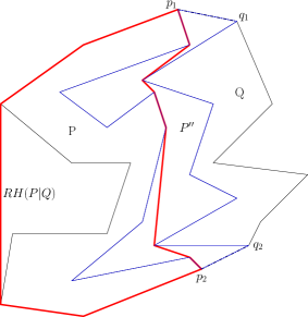
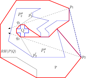
Figure 2: The figure on the left illustrates case (i) in which $Q$ does not lie in one pocket of $P$. This figure also shows the existence of two bridges $p_{1}q_{1}$ and $p_{2}q_{2}$. The simple polygon $P^{\prime\prime}$ is shown in blue. The figure on the right illustrates case (ii) in which $Q$ belongs to a pocket of $P$. The simple polygon $P^{\prime\prime}=P_{1}^{\prime\prime}\cup P_{2}^{\prime\prime}$ is shown in blue. In both the figures, $RH(P|Q)$ is in red.

We call an edge $e$ of $CH(P\cup Q)$ a bridge if one endpoint of $e$ lies on $P$ and the other endpoint lies on $Q$. Given that $P$ and $Q$ are alongside each other, the number of bridges on the boundary of $CH(P\cup Q)$ is either zero or two. Indeed, two bridges in $CH(P\cup Q)$ signify case (i), whereas the zero number of bridges indicates case (ii). Refer to Fig. 2. By applying Jarvis’s march to vertices in $P\cup Q$, we compute the edges of $CH(P\cup Q)$ until either two bridges are found or $CH(P\cup Q)$ is computed. From this, we determine whether the algorithm needs to handle either case (i) or case (ii). In case (i), our algorithm stores the bridges, $p_{1}q_{1}$ and $p_{2}q_{2}$, with $p_{1},p_{2}\in P$ and $q_{1},q_{2}\in Q$.

First, we present an algorithm to handle case (i). Consider the simple polygon $P^{\prime\prime}$ to the right of bridge from $p_{1}$ to $q_{1}$, the right of the section of $bd(Q)$ that occurs in traversing the $bd(Q)$ in counterclockwise direction from $q_{1}$ to $q_{2}$, the right of bridge from $q_{2}$ to $p_{2}$, and to the right of section of $bd(P)$ that occurs in traversing the $bd(P)$ in counterclockwise direction from $p_{2}$ to $p_{1}$. Refer to the left subfigure of Fig. 2. Also, let $SP_{P^{\prime\prime}}(p_{1},p_{2})$ be the shortest path from $p_{1}$ to $p_{2}$ in $P^{\prime\prime}$. The $RH(P|Q)$ is the simple polygon to the right of $SP_{P^{\prime\prime}}(p_{1},p_{2})$ and to the right of the section $S(p_{2},p_{1})$ of $bd(CH(P))$ that occurs in traversing the $bd(CH(P))$ in clockwise direction from $p_{2}$ to $p_{1}$. Starting at $p_{2}$, using Jarvis’s march, we compute the edges of $S(p_{2},p_{1})$, until $p_{1}$ is encountered. This takes $O(|P|^{2})$ time and uses $O(1)$ workspace. For computing the shortest path from $p_{1}$ to $p_{2}$ in $P^{\prime\prime}$, we use the constant workspace algorithm presented in Section 2, except that $P^{\prime\prime}$ here is formed by a contiguous section of $bd(P)$, a contiguous section of $bd(Q)$, and two line segments (bridges). In initiating a cone with apex at $p_{1}$, extending a ray of any cone, modifying any cone to another, and locating $p_{2}$ relative to any cone, the algorithm presented in Section 2 is modified to consider $P^{\prime\prime}$ described herewith.

Lemma 1

Given $P$ and $Q$, determining that $Q$ does not lie in any pocket of $P$ together with computing $RH(P|Q)$ takes $O(|P|^{2}+|Q|^{2})$ time using $O(1)$ workspace.

Proof

Computing the two bridges via Jarvis’s march on the vertices of $P\cup Q$ takes $O(|P|^{2}+|Q|^{2})$ time. For computing the $S(p_{2},p_{1})$, Jarvis’s march on the vertices of $P$ takes $O(|P|^{2})$ time. The algorithm presented in Section 2 to compute the $SP_{P^{\prime\prime}}(p_{1},p_{2})$ takes $O(|P|^{2}+|Q|^{2})$ time. Since the Jarvis’s march uses $O(1)$ workspace, and since the algorithm in Section 2 also takes $O(1)$ workspace, this algorithm uses constant workspace. Also, the vertices of $RH(P|Q)$ are output as and when they are determined.

When there is no bridge on the $bd(CH(P\cup Q))$, the input falls into the case (ii). In this case, our algorithm finds the pocket in which $Q$ resides. For any simple polygon $P^{\prime}$ and a point $q^{\prime}$, it is well-known that $q^{\prime}$ belongs to the relative interior of $P^{\prime}$ if and only if the number of intersections of the horizontal line passing through $q^{\prime}$ with $P^{\prime}$ to the left of $q^{\prime}$ is odd. Let $q$ be any vertex of $Q$. We compute the $bd(CH(P))$ using Jarvis’s march on the vertices of $P$, starting from any vertex of $P$. As and when any edge $p_{1}p_{2}$ of $bd(CH(P))$ is determined, we check whether that edge defines a pocket $P^{\prime}$. If it is, starting from $p_{1}$, we traverse the $bd(P^{\prime})$ and count the number of times the horizontal line through $q$ intersects with the $bd(P^{\prime})$ to the left of $q$. If this number is odd, then $Q$ belongs to $P^{\prime}$. Otherwise, we continue computing the $bd(CH(P))$ with Jarvis’s march, starting from $p_{2}$. This process is guaranteed to terminate since $Q$ has already been found to be in one of $P$’s pockets.

Let $p_{1}$ and $p_{2}$ be the endpoints of the lid of a pocket $P^{\prime}$ in which $Q$ resides such that $p_{2}$ occurs next to $p_{1}$ in traversing the $bd(CH(P))$ in the clockwise direction. Then, $P^{\prime\prime}=P^{\prime}\backslash Q$ is a simple polygon with hole $Q$. To facilitate finding shortest paths using the constant workspace algorithm presented in Section 2, as described below, we partition $P^{\prime\prime}$ into two simple polygons $P_{1}^{\prime\prime}$ and $P_{2}^{\prime\prime}$. Refer to the right subfigure of Fig. 2. First, we find the point of tangency $q_{1}$ (resp. $q_{2}$) of $Q$ from $p_{1}$ (resp. $p_{2}$) such that the half-plane $H_{1}$ (resp. $H_{2}$) defined by the line induced by $p_{1}q_{1}$ (resp. $p_{2}q_{2}$) contains $Q$. Then, we traverse the $bd(P^{\prime\prime})$ to find a vertex $p_{1}^{\prime}$ of $P^{\prime}$ located in $\overline{H_{1}}$ such that the line segment $q_{1}p_{1}^{\prime}\in P^{\prime\prime}$. For every vertex $p^{\prime\prime}$ of $bd(P^{\prime})$ that is located in $\overline{H_{1}}$, we check whether any edge of $P^{\prime}$ intersects with the line segment $q_{1}p^{\prime\prime}$. If not, then that $p^{\prime\prime}$ is defined to be $p_{1}^{\prime}$. Since $bd(P^{\prime})$ is a cycle, such a $p_{1}^{\prime}$ is guaranteed to exist in $\overline{H_{1}}$. Finding $p_{1}^{\prime}$ takes $O(|P^{\prime}|^{2})$ time using $O(1)$ workspace. Analogously, we find a vertex $p_{2}^{\prime}$ of $P^{\prime}$ in $\overline{H_{2}}$ such that the line segment $q_{2}p_{2}^{\prime}$ is in $P^{\prime\prime}$ and its interior does not intersect with any edge of $P^{\prime}$.

The closed region bounded by line segment $p_{1}p_{2}$, polygonal chain from $p_{2}$ to $p_{2}^{\prime}$ along $bd(P^{\prime})$ when the $bd(P^{\prime})$ is traversed in clockwise direction, line segment $p_{2}^{\prime}q_{2}$, polygonal chain from $q_{2}$ to $q_{1}$ along $bd(Q)$ when the $bd(Q)$ is traversed in counterclockwise direction, line segment $q_{1}p_{1}^{\prime}$, and the polygonal chain from $p_{1}^{\prime}$ to $p_{1}$ along $bd(P^{\prime})$ when the $bd(P^{\prime})$ is traversed in clockwise direction is the simple polygon $P_{1}^{\prime\prime}$. We denote the simple polygon $P^{\prime\prime}-P_{1}^{\prime\prime}$ by $P_{2}^{\prime\prime}$. Then, we compute three shortest paths, each with a constant workspace algorithm presented in Section 2: one between $p_{1}$ and $q_{1}$ in $P_{1}^{\prime\prime}$, one between $q_{1}$ and $q_{2}$ in $P_{2}^{\prime\prime}$, and the last one between $q_{2}$ and $p_{2}$ in $P_{1}^{\prime\prime}$. As the vertices of these shortest paths are computed, our algorithm outputs them. We note that those vertices shared by the shortest path from $p_{1}$ to $q_{1}$ and the shortest path from $p_{2}$ to $q_{2}$ are output two times; however, this does not affect the correctness. Starting from $p_{1}$, by applying Jarvis’s march to vertices of $P$, we compute the $bd(CH(P))$ in the counterclockwise direction until Jarvis’s march outputs $p_{2}$. As each edge of this section of $bd(CH(P))$ is determined, we output it.

Lemma 2

Given $P$ and $Q$, determining that $Q$ lies in a pocket of $P$ together with computing $RH(P|Q)$ takes $O(|P|^{2}+|Q|^{2})$ time using $O(1)$ workspace.

Proof

To determine that there are no bridges on the $bd(CH(P\cup Q))$ involves computing the $CH(P\cup Q)$ with Jarvis’s march on the vertices of $P\cup Q$, which takes $O(|P|^{2}+|Q|^{2})$ time using $O(1)$ workspace. With Jarvis’s march on the vertices of $P$, computing the $CH(P)$ takes $O(|P|^{2})$ time. For every edge $e$ computed on the $bd(CH(P))$, determining whether $e$ is the lid of a pocket takes $O(1)$ time. If $e$ is found to be a lid of the pocket $P^{\prime}$, determining whether $Q$ lies in the pocket defined by $e$ takes $O(|P^{\prime}|)$ time using $O(1)$ workspace: this involves locating a vertex $q$ of $Q$, by checking the number of intersections of $bd(P^{\prime})$ with the horizontal line passing through $q$. Finding the pocket containing the $Q$ takes $O(|P|)$ time using $O(1)$ workspace. Finding the point of tangency $q_{1}$ on $bd(Q)$ from $p_{1}$ takes $O(|Q|^{2})$ time using $O(1)$ workspace as we need to check whether $p_{1}q$ supports $Q$ for every vertex $q$ of $p_{1}$. Analogously, computing the point of tangency $q_{2}$ on $bd(Q)$ from $p_{2}$ takes $O(|Q|^{2})$ time using $O(1)$ workspace. As explained, finding vertices $p_{1}^{\prime}$ and $p_{2}^{\prime}$ on $P$ takes $O(|P^{\prime}|^{2})$ time using $O(1)$ space. Computing three shortest paths, two in $P_{1}^{\prime\prime}$ and one in $P_{2}^{\prime\prime}$, using the algorithm in Section 2, takes $O(|P^{\prime}|^{2}+|Q|^{2})$ time. Since these simple polygons are not saved in memory, instead, a vertex or a point on the edge of a simple polygon is computed as and when needed, computing these shortest paths uses $O(1)$ workspace. Further, the vertices of these shortest paths are output as and when they are determined. Computing the section of $bd(CH(P))$ from $p_{1}$ to $p_{2}$ in counterclockwise direction takes $O(|P|^{2})$ time.

Theorem 3.1

Given two simple polygons $P$ and $Q$, with $Q$ located alongside $P$, the algorithm described above correctly computes $RH(P|Q)$ in $O(|P|^{2}+|Q|^{2})$ time using $O(1)$ workspace.

Proof

The time and workspace complexities are due to Lemmas 1 and 2. The correctness is immediate from the above presentation and due to the algorithm in [24].

4 Relative hull of points located in a simple polygon

In this section, we seek to find the relative hull of a set $S$ of points located in the simple polygon $P$. Our algorithm outputs a weakly simple polygon $RH(S|P)$ with a perimeter of minimum length that lies in the relative interior of $P$ and contains all the points in $S$. For this problem, Toussaint [23] proposed an algorithm, that takes $O(|S|\lg{|S|})$ time in the worst-case while using $O(|P|+|S|)$ workspace. This result first finds a weakly simple polygon $P^{\prime}$ like ours, and then it transforms $P^{\prime}$ to a simple polygon by reducing the latter problem to finding the geodesic shortest path in $P\backslash P^{\prime}$. The constant workspace algorithm presented herewith computes only the weakly simple polygon with a perimeter of minimum length.

For this problem, the algorithm in [23] computes a triangulation of $P$. The Eulerian tour of the dual graph of that triangulation is used to visit triangles of that triangulation. Whenever a triangle is visited, the convex hull of points of $S$ located in that triangle is computed. For every two hulls that occur next to each other in the Eulerian tour of the dual graph, a geodesic shortest path is computed to join the two special points (of $S$) on those two hulls. As claimed in [23], those hulls and the shortest paths computed together form a weakly simple polygon, and this polygon is further transformed into a simple polygon.

While following the outline of algorithm given in [23] for this problem, here we devise a constant workspace algorithm using algorithmic ideas from Asano et al. [5]. These include on-the-fly computation of constrained Delaunay triangulation of the input simple polygon $P$, denoted by $CDT(P)$, an algorithm to visit the triangles of $CDT(P)$ using the Eulerian walk of dual tree corresponding to $CDT(P)$, and computing the geodesic shortest path between the chosen points of $S$ in a sleeve of triangles. And, like in algorithms presented in previous sections, we use Jarvis’s march [17] (also presented in [21]) to compute sections of boundaries of convex hulls of subsets of points of $S$.

First, we define $CDT(P)$ from [5]. For any edge $pq$ of $CDT(P)$ and a vertex $r$ of $P$ distinct from $p$ and $q$, the triangle $pqr$ belongs to $CDT(P)$ if and only if (i) $r$ is visible from both $p$ and $q$, and (ii) the circle defined by $p,q$, and $r$ does not contain any other vertex of $P$ that is visible from $r$. It is well-known that $CDT(P)$ is unique for any simple polygon $P$. The dual of $CDT(P)$ is the graph $T$ obtained by introducing a node for each triangle of $CDT(P)$ and introducing an edge between any two nodes whenever their corresponding triangles are adjacent along an edge of $CDT(P)$. It is known that since $P$ is a simple polygon, the graph $T$ is indeed a tree. Hence, we call $T$ as the dual-tree of $CDT(P)$.

Like in [5], our algorithm computes a triangle of $CDT(P)$ on the fly, that is, as and when that triangle is needed. Since $T$ is not stored, as part of computing the Eulerian tour $\tau$ of $T$, our algorithm computes the triangles of $CDT(P)$ one after the other in an online fashion. That is, given an edge $e$ of $CDT(P)$, the triangles to which $e$ is incident in $CDT(P)$ are computed. The on-the-fly computation of $CDT(P)$ is also needed whenever the geodesic shortest path is required to be computed between any two chosen points of $S$. Since $CDT(P)$ is unique for $P$, re-computing the triangles of interest in $CDT(P)$ always yield the identical set of triangles. Also, the dual-tree $T$ associated with $CDT(P)$ is unique; hence, re-computing edges incident to any node of $T$ yields the same set of edges. Though the weakly simple polygon with a perimeter of minimum length for the given $S$ and $P$ is not necessarily unique, since the $CDT(P)$ is unique, our algorithm always outputs the same weakly simple polygon.

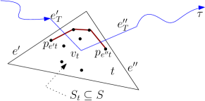
Figure 3: The section of the boundary of the convex hull of the set $S_{t}\subseteq S$ of points located in triangle $t$ between the connecting point $p_{e^{\prime}t}$ of $e^{\prime}$ in $t$ and the connecting point $p_{e^{\prime\prime}t}$ of $e^{\prime\prime}$ in $t$ is illustrated in red. The Eulerian tour $\tau$ of the dual-tree $T$ of $CDT(P)$ is illustrated in blue. Here, $v_{t}$ is the dual vertex corresponding to triangle $t$. Also, $e^{\prime}$ and $e^{\prime\prime}$ of $CDT(P)$ respectively correspond to edges $e_{T}^{\prime}$ and $e_{T}^{\prime\prime}$ of the dual-tree $T$.

For every triangle $t\in CDT(P)$ that has points from $S$, for every edge $e$ of $t$, among all the points belonging to $S$ that are located in $t$, following [23], the one closest to $e$ is called the connecting point of $e$ in $t$, denoted by $p_{et}$. We say a triangle $t$ is visited whenever the Eulerian tour $\tau$ of $T$ visits the dual node $v_{t}$ of $T$ corresponding to $t$. Since the degree of any node in $T$ is at most three, any triangle $t$ of $CDT(P)$ is visited at most three times. Suppose the tour $\tau$ encounters a node $v_{t}\in T$ by traversing an edge $e_{T}^{\prime}$ of $T$, and leaves $v_{t}$ by traversing an edge $e_{T}^{\prime\prime}$ of $T$, where $e_{T}^{\prime}$ and $e_{T}^{\prime\prime}$ are not necessarily distinct edges of $T$ that are incident to $v_{t}$. Refer to Fig. 3. Let $S_{t}\subseteq S$ be the set of points in $t$. If $|S_{t}|>0$ and $e_{T}^{\prime}\neq e_{T}^{\prime\prime}$, then our algorithm computes the section of $bd(CH(S_{t}))$ from $p_{e^{\prime}t}$ to $p_{e^{\prime\prime}t}$ using Jarvis’s march, where $e^{\prime}$ is the dual edge of $CDT(P)$ corresponding to $e_{T}^{\prime}$ and $e^{\prime\prime}$ is the dual edge of $CDT(P)$ corresponding to $e_{T}^{\prime\prime}$. As part of computing these hull edges, to determine points in $S$ belonging to $t$, we traverse the input array comprising points in $S$. After Jarvis’s march computes every edge, that edge is sent to the output stream.

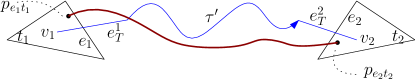
Figure 4: Illustrates the geodesic shortest path (in red) from connecting point $p_{e_{1}t_{1}}$ to connecting point $p_{e_{2}t_{2}}$. The subtour $\tau^{\prime}$ between triangles $t_{1}$ and $t_{2}$ in the dual-tree $T$ is in blue. Here, $v_{1}$ and $v_{2}$ are dual vertices corresponding to triangles $t_{1}$ and $t_{2}$. Also, triangulation edges $e_{1}$ and $e_{2}$ respectively correspond to edges $e_{T}^{1}$ and $e_{T}^{2}$ in the dual-tree $T$.

Let $t_{1}$ and $t_{2}$ be any two triangles such that both $t_{1}$ and $t_{2}$ have points from $S$, triangle $t_{2}$ is visited after visiting triangle $t_{1}$, and no triangle with points from $S$ is visited between these visits of $t_{1}$ and $t_{2}$. Let $\tau^{\prime}$ be the shortest contiguous section of Eulerian tour $\tau$ corresponding to this traversal of $T$. Let $v_{1}$ and $v_{2}$ be the vertices in $T$ corresponding to $t_{1}$ and $t_{2}$, respectively. In $\tau^{\prime}$, let $e_{T}^{1}$ be the edge incident to $v_{1}$ and $e_{T}^{2}$ be the edge incident to $v_{2}$. Let $e_{1}$ and $e_{2}$ be the dual edges of $CDT(P)$ corresponding to $e_{T}^{1}$ and $e_{T}^{2}$. Then, we find the geodesic shortest path between connecting points $p_{e_{1}t_{1}}$ and $p_{e_{2}t_{2}}$ in the sleeve comprising all the triangles of $CDT(P)$ that are visited in $\tau^{\prime}$. We note that sleeve is a simply connected region formed by any contiguous sequence of triangles such that there is a simple path in $T$ that precisely comprises the dual nodes of these triangles. To facilitate computing this geodesic shortest path, after visiting $t_{1}$ in $\tau^{\prime}$, our algorithm stores both the $t_{1}$ and the $p_{e_{1}t_{1}}$. Refer to Fig. 4. Again, we note that instead of storing edges of that shortest path, our algorithm outputs as soon as any edge of that shortest path is computed.

The main overhead in visiting any triangle $t$ of $CDT(P)$ is computing the $t$ itself, that is, before visiting $t$. Let $pq$ be an edge of triangle $pqr^{\prime}\in CDT(P)$. Then, computing the triangle of $CDT(P)$ that shares edge $pq$ with $pqr^{\prime}$ involves finding a vertex $r$ of $P$ such that $pqr$ obeys the definition of being a triangle belonging to $CDT(P)$. For any given vertex $s\in P$, the algorithm needs to determine (i) whether the interior of $ps$ intersects with any edge of $P$, (ii) whether the interior of $qs$ intersects with any edge of $P$, (iii) for every vertex $s^{\prime}$ belonging to circle passing through $p,q$, and $s$, needs to check whether the interior of $s^{\prime}s$ intersects with any edge of $P$. In determining vertex $r$, these checks can be done in $O(|P|^{2})$ time using $O(1)$ workspace.

In computing the Eulerian tour $\tau$, the adjacent triangle of any triangle of $CDT(P)$ is computed in an online fashion. Since each triangle is visited at most three times, computing all the triangles in the Eulerian tour takes $O(|P|^{3})$ time using $O(1)$ workspace. In addition, to find the geodesic shortest path between two connecting points, we compute the sleeve. This also requires computing the triangles belonging to that sleeve on the fly. Since all the triangles in each such sleeve are computed only once and since the union of triangles in all such sleeves is a subset of triangles of $CDT(P)$, the time to compute all the triangles of $CDT(P)$ that belong to all sleeves together is $O(|P|^{3})$. Excluding the time complexity to compute triangles of $CDT(P)$, computing the Euclidean tour takes $O(|P|)$ time. Since every edge of $P$ is an edge of some triangle in $CDT(P)$, our algorithm starts with an arbitrary edge $p^{\prime}q^{\prime}$ of $P$ and finds the triangle $p^{\prime}q^{\prime}r^{\prime}$ belonging to $CDT(P)$. The Eulerian tour terminates upon visiting all the neighbours of triangle $p^{\prime}q^{\prime}r^{\prime}$.

This leaves us to analyze the time complexity to compute a geodesic shortest path in a sleeve. Applying the algorithm presented in Section 3.1 of [5], the geodesic shortest path computation in a sleeve with $k$ triangles takes $O(k^{3})$ time. Note that this also includes the time to compute the triangles of $CDT(P)$ belonging to that sleeve as and when needed.

Though our algorithm engineers a solution by stitching several constant workspace algorithms together, since the outline of our algorithm is the same as in Toussaint [23], our algorithm is guaranteed to output the same weakly simple polygon as the first phase of the algorithm in [23] outputs for this problem. Below, we provide a proof of correctness and the analysis of our algorithm.

Theorem 4.1

Given a set $S$ points located in the simple polygon $P$, our algorithm computes $RH(S|Q)$ in $O(|P|^{3}+|S|^{2})$ time using $O(1)$ workspace.

Proof

Since the Eulerian tour $\tau$ of the dual-tree $T$ visits every node of $T$ by computing the corresponding triangles of $CDT(P)$ on the fly, every triangle of $CDT(P)$ with points from $S$ is considered. Since the maximum degree of any node of a dual-tree is three, any triangle is visited at most three times. For any triangle $t$ that has a non-empty set $S_{t}\subseteq S$ of points, if $t$ is visited by entering via $e^{\prime}$ and exited $t$ via edge $e^{\prime\prime}$, then the section of $bd(CH(S_{t}))$ between connecting points $p_{e^{\prime}t}$ and $p_{e^{\prime\prime}t}$ is correctly computed using Jarvis’s march. Considering the number of times $t$ is visited and the edges through which $t$ is entered and exited in each of those times, the $bd(CH(S_{t}))$ is guaranteed to be computed correctly. For any two triangles $t^{\prime},t^{\prime\prime}$, there is a unique path between nodes corresponding to them in $T$. And, for every two successive non-empty triangles $t_{1},t_{2}$ along that path, algorithm in [5] correctly computes the geodesic shortest path joining the connecting points $p_{e_{1}t_{1}}$ and $p_{e_{2}t_{2}}$; these connecting points respectively correspond to edge through which $t_{1}$ is exited and the edge through which the tour $\tau$ entered $t_{2}$. This shortest path computation is again accomplished by computing the triangles of $CDT(P)$ on the fly along the sleeve between $t_{1}$ and $t_{2}$. These triangles are computed correctly since we use the naive algorithm to compute triangles of $CDT(P)$. Considering the correctness of algorithm for this problem in [23], the computation of weakly simple polygon is correct.

Given a triangle $t$ and an edge $e$ of $t$, computing a triangle in $CDT(P)$ adjacent to $t$ that has $e$ on its boundary takes $O(|P|^{2})$ time. Since the triangulation is not stored and computed on the fly, given there are $O(n)$ triangles in $CDT(P)$, computing the triangles of $CDT(P)$, while computing an Eulerian tour of $T$ takes $O(|P|^{3})$ time using $O(1)$ workspace. The cost of the Eulerian tour, which is $O(|P|)$, is dominated by the cost of this computation. For any triangle $t_{i}$ that has the set $S_{i}\subseteq S$ of points, for every invocation of Jarvis’s march on $S_{i}$, we need to find points that belong to $t_{i}$ by traversing the list of points in $S$. Hence, Jarvis’s march to compute any one edge of the hull of points in $S_{i}$ takes $O(|S|)$ time. Excluding the time to compute the Euclidean tour of $T$, the time for computing all such hulls together takes $\sum_{t_{i}\text{ contains points from $S$}}(|S|\cdot|S_{i}|)$ time, which is $O(|S|^{2})$. Further, using a constant workspace, computing all the shortest paths between connecting points together takes $O(k^{2})$ time, where $k$ is the number of triangles belonging to that sleeve. Since the sum of the number of triangles in all such sleeves is $O(|P|)$, the costs of all shortest path computations together take $O(|P|^{2})$ time. The computation of triangles of $CDT(P)$ as part of these shortest path computations again takes $O(|P|^{3})$ time using $O(1)$ workspace.

5 Conclusions

This paper attempted to devise constant workspace algorithms for three problems: (i) relative hull of a simple polygon $P$ located in another simple polygon $Q$, (ii) relative hull of a simple polygon $P$ placed alongside another simple polygon $Q$, and (iii) the relative hull of a set $S$ of points located in a simple polygon $P$. For the first two problems, we proposed $O(|P|^{2}+|Q|^{2})$ time solutions using constant workspace. The algorithm presented for the last problem has $O(|P|^{3}+|S|^{2})$ time complexity while using constant workspace. We feel the cubic dependence on $|P|$ can possibly be reduced to quadratic with a little more research. Also, like in [23], extending this algorithm to output a simple polygon, instead of a weakly simple polygon, while using a constant workspace would be interesting. This work is the first attempt to find space-efficient algorithms for computing relative hulls. Of course, providing time-workspace trade-offs for all these problems would also be interesting. As an extension to the last problem, it would be interesting to compute the relative hull of a set of points when these points are located amidst line segments using a constant workspace.

Acknowledgement

This research of R. Inkulu is supported in part by the National Board for Higher Mathematics (NBHM) grant 2011/33/2023NBHM-R&D-II/16198.

References

- [1] M. Abrahamsen. An optimal algorithm for the separating common tangents of two polygons. In International Symposium on Computational Geometry, pages 198–208, 2015.
- [2] B. Aronov, M. Korman, S. Pratt, A. van Renssen, and M. Roeloffzen. Time-space trade-off algorithms for triangulating a simple polygon. Journal of Computational Geometry, pages 105–124, 2017.
- [3] T. Asano, K. Buchin, M. Buchin, M. Korman, W. Mulzer, G. Rote, and A. Schulz. Memory-constrained algorithms for simple polygons. Computational Geometry, pages 959–969, 2013.
- [4] T. Asano, W. Mulzer, G. Rote, and Y. Wang. Constant-work-space algorithms for geometric problems. Journal of Computational Geometry, pages 46–68, 2011.
- [5] T. Asano, W. Mulzer, and Y. Wang. Constant workspace algorithms for shortest paths in trees and simple polygons. Journal of Graph Algorithms and Applications, pages 569–586, 2011.
- [6] Y. Bahoo, B. Banyassady, P. K. Bose, S. Durocher, and W. Mulzer. A time–space trade-off for computing the -visibility region of a point in a polygon. Theoretical Computer Science, 789:13–21, 2019.
- [7] B. Banyassady, L. Barba, and W. Mulzer. Time-space trade-offs for computing Euclidean minimum spanning trees. Journal of Computational Geometry, 11(1):525–547, 2020.
- [8] B. Banyassady, M. Korman, and W. Mulzer. Computational geometry column 67. ACM SIGACT News, 49(2):77–94, 2018.
- [9] B. Banyassady, M. Korman, W. Mulzer, A. van Renssen, M. Roeloffzen, P. Seiferth, and Y. Stein. Improved time-space trade-offs for computing Voronoi diagrams. Journal of Computational Geometry, 9(1):191–212, 2018.
- [10] L. Barba, M. Korman, S. Langerman, K. Sadakane, and R. I. Silveira. Space-time trade-offs for stack-based algorithms. Algorithmica, pages 1097–1129, 2015.
- [11] B. Bronnimann, T. M. Chan, and E. Y. Chen. Towards in-place geometric algorithms and data structures. In International Symposium on Computational Geometry, pages 239–246, 2004.
- [12] H. Bronnimann, J. Iacono, J. Katajainen, P. Morin, J. Morrison, and G. T. Toussaint. In-place planar convex hull algorithms. In Proceedings of Latin American Theoretical Informatics, pages 494–507, 2002.
- [13] T. M. Chan. Optimal output-sensitive convex hull algorithms in two and three dimensions. Discrete & Computional Geometry, pages 361–368, 1996.
- [14] O. Darwish and A. Elmasry. Optimal time-space tradeoff for the 2d convex-hull problem. In European Symposium on Algorithms, pages 284–295, 2014.
- [15] M. de Berg, O. Cheong, M. van Kreveld, and M. Overmars. Computational Geometry: Algorithms and Applications. Springer-Verlag, 2008.
- [16] S. Har-Peled. Shortest path in a polygon using sublinear space. In International Symposium on Computational Geometry, pages 111–125, 2015.
- [17] R.A. Jarvis. On the identification of the convex hull of a finite set of points in the plane. Information Processing Letters, pages 18–21, 1973.
- [18] D. G. Kirkpatrick and R. Seidel. The ultimate planar convex hull algorithm? SIAM Journal on Computing, 15(1):287–299, 1986.
- [19] G. Klette. A recursive algorithm for calculating the relative convex hull. In International Conference on Image and Vision Computing, pages 1–7, 2010.
- [20] M. Korman, W. Mulzer, A. van Renssen, M. Roeloffzen, P. Seiferth, and Y. Stein. Time-space trade-offs for triangulations and Voronoi diagrams. Computational Geometry, 73:35–45, 2018.
- [21] F. P. Preparata and M. I. Shamos. Computational Geometry: an Introduction. Springer-Verlag, New York, USA, 1985.
- [22] O. Reingold. Undirected connectivity in log-space. Journal of the ACM, 55(4):1–24, 2008.
- [23] G. T. Toussaint. An optimal algorithm for computing the relative convex hull of a set of points in a polygon. EURASIP, Signal Processing III: Theories Applications, Part 2, pages 853–856, 1986.
- [24] G. T. Toussaint. On separating two simple polygons by a single translation. Discrete & Computational Geometry, pages 265–278, 1989.
- [25] P. Wiederhold and H. Reyes. Relative convex hull determination from convex hulls in the plane. Combinatorial Image Analysis, pages 46–60, 2016.