Efficient Depth Estimation for Unstable Stereo Camera Systems on AR Glasses

Abstract

Stereo depth estimation is a fundamental component in augmented reality (AR) applications. Although AR applications require very low latency for their real-time applications, traditional depth estimation models often rely on time-consuming preprocessing steps such as rectification to achieve high accuracy. Also, non standard ML operator based algorithms such as cost volume also require significant latency, which is aggravated on compute resource-constrained mobile platforms. Therefore, we develop hardware-friendly alternatives to the costly cost volume and preprocessing and design two new models based on them, MultiHeadDepth and HomoDepth. Our approaches for cost volume is replacing it with a new group-pointwise convolution-based operator and approximation of consine similarity based on layernorm and dot product. For online stereo rectification (preprocessing), we introduce homograhy matrix prediction network with a rectification positional encoding (RPE), which delivers both low latency and robustness to unrectified images, which eliminates the needs for preprocessing. Our MultiHeadDepth, which includes optimized cost volume, provides 11.8-30.3% improvements in accuracy and 22.9-25.2% reduction in latency compared to a state-of-the-art depth estimation model for AR glasses from industry. Our HomoDepth, which includes optimized preprocessing (Homograhpy + RPE) upon MultiHeadDepth, can process unrectified images and reduce the end-to-end latency by 44.5%. We adopt a multi-task learning framework to handle misaligned stereo inputs on HomoDepth, which reduces theAbsRel error by 10.0-24.3%. The results demonstrate the efficacy of our approaches in achieving both high model performance with low latency, which makes a step forward toward practical depth estimation on future AR devices.

1 Introduction

Depth estimation serves as a foundational component in augmented and virtual reality (AR/VR) [16] with many downstream algorithms, which include novel-view rendering [14, 28], occlusion reasoning [17], world locking for AR object placement [18], and determining the scale of AR objects [3]. In the AR domain, stereo depth estimation is often deployed [28] rather than mono depth estimation due to its superior accuracy and the ease of deploying stereo cameras on the each side of the AR glasses frame. One key objective for depth estimation models targeting AR glasses is the low latency, in addition to the good performance, because many AR use cases are realtime applications [16]. However, since AR glasses are in a compute resource-constrained wearable form factor, enabling desired latency (less than 100 ms on device) is not trivial.

One challenge towards the latency optimization originates from the preprocessing, which is a indispensable step for achieving high model performance in practical applications. Examples include camera distortion and alignment using camera intrinsic and extrinsic. In addition to image preprocessing, depth estimation models often involve traditional algorithms such as cost volume [7, 28]. We present their significance in latency in Fig. 1, which shows that preprocessing accounts for 30.2% and cost volume accounts for 29.3% of the total latency of a state-of-the-art model, Argos [28]. Note that preprocessing latency can be more dominant when camera intrinsic and extrinsic parameters are unknown, which results in 200 to 2000 ms latency to solve for the extrinsic parameters and subsequently process the images [15, 30]. This aggravates the long preprocessing latency challenge further.

Therefore, to reduce depth estimation model latency for AR glasses, we propose new methodologies that significantly reduce the preprocessing (online stereo rectification not required) and cost volume latency, as shown in Fig. 1. Our approach for the cost volume is (1) to replace traditional algorithm with group-pointwise convolutions, which are highly optimized in hardware and compiler and (2) adopt an efficient approximation of consine similarity using layernorm and dot product. For preprocessing (stereo matching), we adopt homography matrix-based approximation and estimate homography using a head attached to the depth estimation model, which allows to utilize homography matrix-based approximation with dynamically varying extrinsic parameters in unstable AR glasses platform or no access to camera extrinsic parameters.

Since our methodologies are complementary to existing depth estimation models, we augment our methodologies on the Argos [28] and develop two versions of new models, MultiHeadDepth and HomoDepth, to show the effectiveness of our methodologies. As presented in Fig. 1, MultiHeadDepth focuses on cost volume optimization, which reduces AbsRel by 7% and inference latency by 25% compared to the original cost volume. HomoDepth targets scenarios that require stereo matching preprocessing, which can directly accept unrectified images as input, eliminating the needs for preprocessing step. HomoDepth not only provides high-quality outputs on unrectified images as presented in Tab. 4, but also significantly reduces the end-to-end latency by 43%. Our evaluation includes ADT [20] dataset collected by real research AR glasses by Meta, Aria [5], which demonstrates the effectiveness of our approach on realistic AR glasses platform.

We summarize our contributions as follows:

• We develop multi-head cost volume block that replaces costly cost volume blocks in previous depth estimation models. Our new block provides significantly lower latency as well as higher accuracy compared to the original cost volume.

• We introduce the homograpghy of stereo images to reveal their position relationship to enable to accept unrectified images without preprocessing. We merge a small homograpghy estimation head within the depth estimation network, which significantly reduces the latency compared to the preprocessing-based approach.

• We augment our homography estimation head with 2D rectification position encoding, which helps translate relative positional information from homograpghy matrix to emdeding coding format. It enables the neural network to effectively understand relative position information, which plays a key role in eliminating the need for rectification preprocessing.

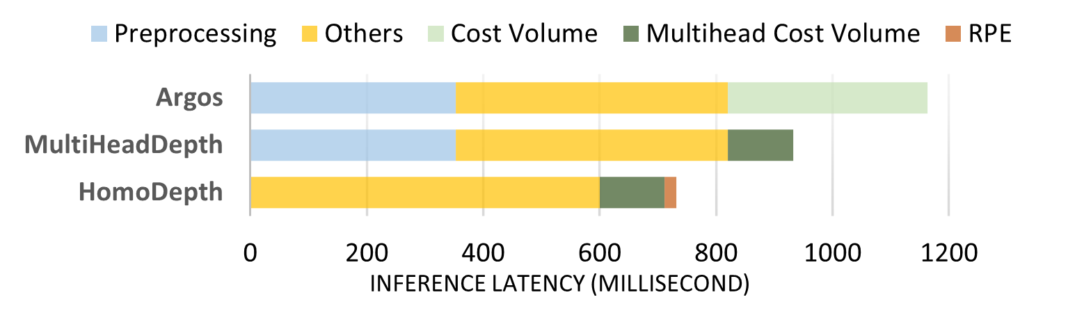
Figure 1: The latency breakdown analysis of a state-of-the-art model Argos [28] and ours, MultiHeadDepth & HomoDepth on Intel Core(TM) i7-12700H CPU (laptop). The ”RPE” refers to the 2D rectification position encoding process. ”Others” refers to all the other part of the neural network excluding cost volume blocks, such as Conv, Norm, FC, and ReLU6.

2 Related Work

Stereo Depth Estimation.

Fast depth estimation on mobile devices is a challenging task. Multiple previous works focused on delivering both model performance and efficiency targeting mobile platforms.

MobileStereoNet [24] is a stereo depth estimation model optimized for mobile devices, featuring a lightweight network design and algorithms specially adapted for stereo matching. However, despite its minimal parameter size, the computational complexity is not small with high FLOPS (e.g. 190G FLOPS), which makes it challenging to achieve efficient performance on mobile platforms.

Argos [28] extended Tiefenrausch monocular network [14] to implement stereo depth estimation. Argos is optimized to minimize the model size and computational complexity. Argos Network consists of encoder, cost volume, and a decoder, which requires preprocesing if the input images are not rectified or distorted. Argos was designed for practical AR applications by Meta, and it delivers state-of-the-art performance in the stereo depth estimation on AR glasses domain.

DynamicStereo [11] is another lightweight design in the parameter size with low latency as well, but Argos delivers superior accuracy and latency.

Stereo Image Preprocessing. The preprocessing of stereo images consists of two parts: Calibration and Rectification. Calibration is required for a raw image captured by the camera, which removes distortion and artifacts in the raw image caused by the imaging system. Sometimes it crops images to remove the black margins around the images. Calibration depends on the intrinsic parameters of camera systems. Generally, the intrinsic of a camera is stable and provided by the manufacturer. Calibration can be completed with just a few matrix computations, requiring only a few dozen milliseconds of hardware.

Rectification is a major challenge in stereo vision systems. For an object in the real world, its projection onto the two image planes should lie on the epipolar lines, satisfying the epipolar constraint [6]. If there is a misalignment between two cameras, it is necessary to rectify the pair of images so that corresponding points lie on the same horizontal line. The stereo cameras are mounted on both sides of AR glasses. The glasses may undergo significant bending ($>10^{\circ}$) because of the soft material. Additionally, this issue is further exacerbated by variations in users’ head sizes and temperatures. [28].

Rectification requires the relative position information of the two cameras. In previous research, taking MobiDepth [30] as an example, it assumed that the relative positions of the cameras had been obtained before the inference phase. It can only process images based on the known position relationship. This is considered as offline rectification. However, in practical applications, the camera positions on AR glasses need to be determined based on a pair of arbitrarily captured images, which results in online rectification.

Karaev et al. [11] set image saturation to a value sampled uniformly between 0 and 1.4 during the model training phase to make the model more robust for stereo images misalignment. But it lacks good interpolation for robustness. Wang et al. proposed a fast online rectification [28]. However, there remains a 15% to 23% chance of failing to rectify the stereo images.

Every stereo-matching algorithm includes a mechanism for evaluating the similarity of image locations. Matching cost is calculated for every pixel over the range of examined disparities, and it’s a commonly used measurement [9].

Kendall et al. [12] adopted deep unary features to compute the stereo matching cost by forming a cost volume. They form a cost volume of dimensionality $height\times weight\times(max\_disparity+1)\times features$ and pack it into a 4D volume. To construct the 4D volume, the algorithm iteratively move one of the images/features horizontally and compare the matching cost in each disparity, as described in Fig. 2(a). The cost volume information is crucial for a neural network to understand the differences between the two feature maps. Although proven effective, the cost volume has a disadvantage in the computational cost that originates from cosine similarity computation described below:

$$D_{cos}(\boldsymbol{a},\boldsymbol{b})=\frac{\boldsymbol{a}\cdot\boldsymbol{b}}{||\boldsymbol{a}||||\boldsymbol{b}||}$$ (1)

where $\boldsymbol{a}$ and $\boldsymbol{b}$ are the vectors of pixels. The numerator is matrix multiplication-optimized hardware- and compiler-friendly since the dot product computation in a batch is matrix multiplication. However, the denominator requires to compute norms pixel by pixel, which is not very friendly to hardware highly optimized for matrix multiplication.

3 MultiHeadDepth Model

Based our observation on the cost volume, we optimize it by approximating cosine similarity with a set of hardware-friendly operations and introduce a new hardware-friendly block, multi-head cost volume, to replace the overall cost volume algorithm.

3.1 Approximating Cosine Similarity

The cosine similarity calculates the angle between two vectors, which indicates the similarity of the vectors. Since the denominator needs to be optimized as we discussed in Sec. 2, we focus on the denominator. Our approach is replacing the division by denominator in  Eq. 1 with 2D layer normalization (layer norm) since this approach reduces the computational complexity and achieves normalization effect (i.e., the elements within a pixel vector have a mean of zero and a standard deviation of one). Maintaining the numerator (dot product) as is in the modified distance metric, the computational complexity is reduced, as discussed in Sec. 7.1. Although the new metric is not mathematically equivalent as the original cosine similarity, but our evaluation results indicate that the metric is effective.

Another benefit of the layer norm is that it provides a buffer for the cost volume block, enabling it to accept additional encoded information. The pixel of input activation is normalized so that it can be merged with other encodings. For instance, it can handle positional encoding, which will be introduced in Sec. 4.4.

3.2 Multi-head Cost Volume

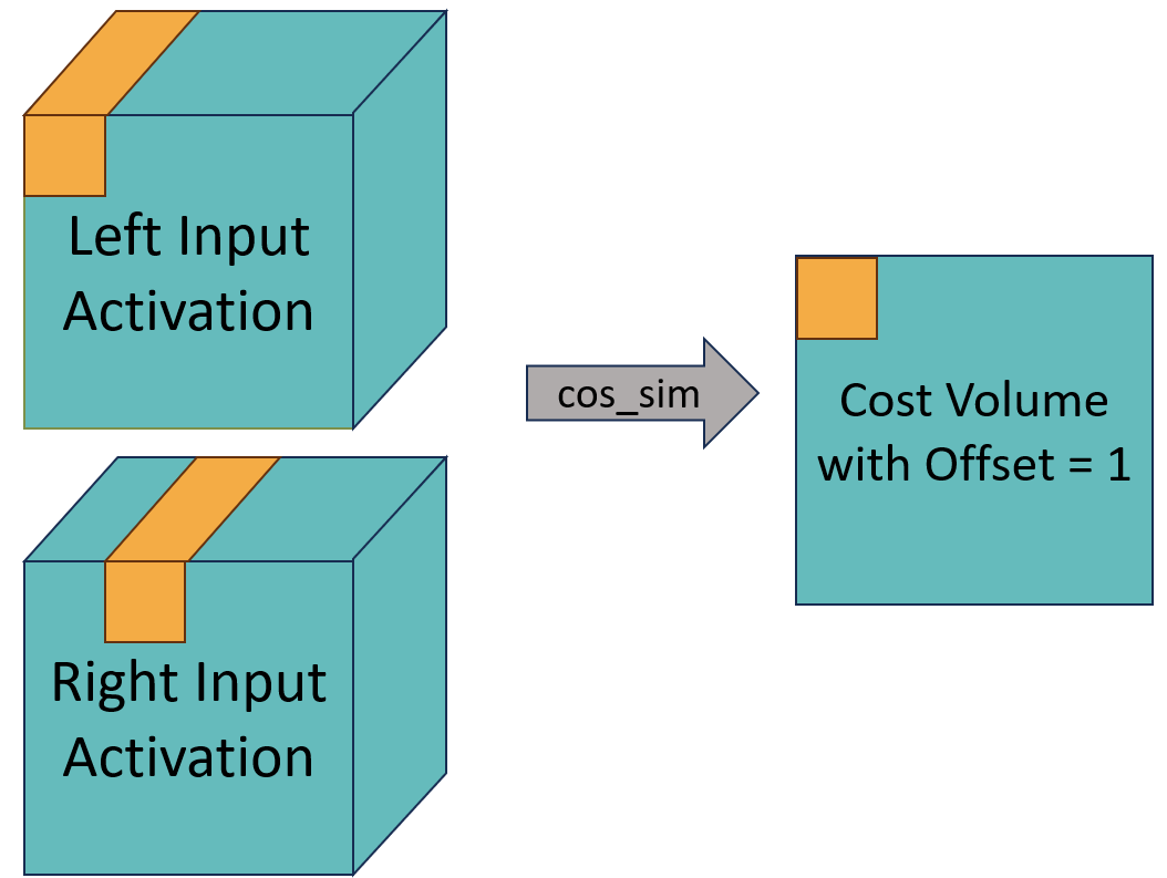
(a) Diagram of the cost volume with an offset of 1. The orange blocks indicate pixel vectors in the input activations, whose size is $1\times number\_of\_channels$.

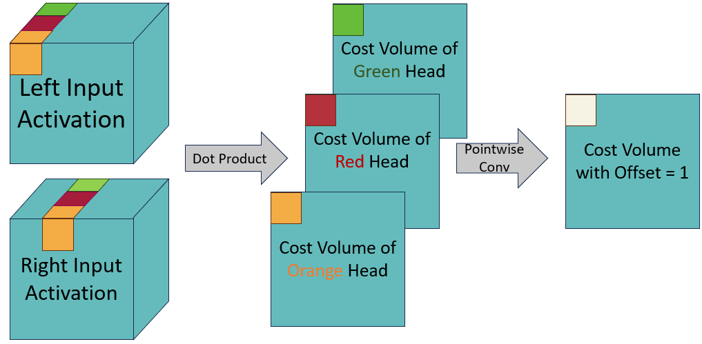
(b) Diagram of the multi-head cost volume (3 heads in this case) with an offset of 1. The orange blocks indicate part of pixel vectors, whose size is $1\times\frac{number\_of\_channels}{number\_of\_heads}$.
 

Figure 2: The comparison between the original and multi-head cost volume

Inspired by multi-head attention mechanism [26], we introduce the multi-head attention and dot scale into the cost volume block since separating the input activation in multiple heads can enable more perceptions of the network. The original cost volume calculates the cosine similarity of pixel vectors of two input activations, and the output is scalar, as shown in Fig. 2(a). The multi-head cost volume computes dot products to produce numerous scalars, forming new pixel vectors. Subsequently, we apply point-wise convolution to generate an output that matches the size of the original cost volume, as Fig. 2(b) shows. Overall, these operations can be executed just by group-wise Conv, which is highly optimized in modern GPUs. The pseudo-code of multi-head cost volume is shown as Algorithm 1.

Algorithm 1 Multi-head Cost Volume

$left:[NCHW]$

$right:[NCHW]$

$max\_disparity:int$

$head\_num:int$ $\triangleright$ number of heads, can divide C

$cost\_volume:[N,max\_disparity,H,W]$

$s=C/head\_num$ $\triangleright$ stride of each head

$left\_norm=\text{LayerNorm}(left)$

$right\_norm=\text{LayerNorm}(right)$

for $i\in 1:max\_disparity+1$ do

    $right\_shifted=\text{roll}(right\_norm,i)$

    for $h\in 0:head\_num$ do

         $left\_slice=left\_norm[:,hs:(h+1)s,:,:]$

         $right\_slice=right\_shifted[:,hs:(h+1)s,:,:]$

         $similarity[:,h,:,:]=\text{dot}(left\_slice,right\_slice)$

         $cost\_volume[:,i,:,:]=\text{pointwise\_conv}(similarity)$

    end for

end for

* In real code, the second loop and pointwise_conv are replaced by the memory operations and group-pointwise convolution

The benefits of multi-head cost volume can be summarized with (1) less computational complexity, (2) replacing the computation with highly-optimized group-wise Conv, and (3) potential accuracy improvement by providing more perceptions of the input activations

3.3 Structure of MultiHeadDepth

Applying our approaches discussed in Sec. 3.1 and Sec. 3.2 to Argos [28], we design MultiHeadDepth, which is illustrated in Fig. 3. All settings for the inverted residual blocks [23] in Argos are retained to highlight the efficacy of our Multi-head Cost Volume in an ablation study. Note that our approach can be applied to other models with cost volume as well.

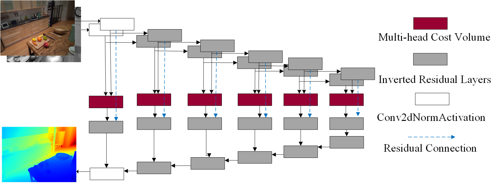
Figure 3: The structure of MultiHeadDepth. The dashed lines indicate that the input activations from the left image are passed to the decoders. The input example is from ADT dataset

4 HomoDepth Model

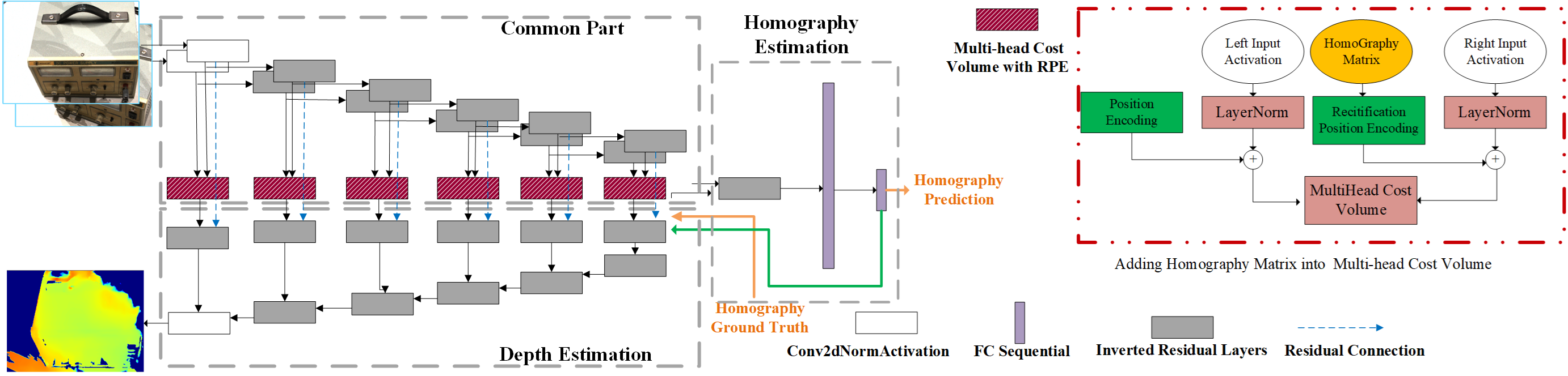
Figure 4: Structure of HomoDepth. The orange connections are only valid in training phase; the green connection is only valid in inference phase. The input example is from DTU dataset.

We discuss how we can augment MultiHeadDepth to include opitmizations for preprocessing process, which consists of the introduction of 3D projection and homographic matrix with homography estimation head.

4.1 3D Projection & Homographic Matrix

The main functionality of cost volume is stereo-matching, which evaluates the similarity of left and right inputs with different offsets to determine the possible disparity. Because the algorithm only allows horizontal offsets, it can only match patterns on a common horizontal line. Therefore, preprocessing is required for the input images for stereo cameras without good alignments.

We will discuss depth estimation from a broader perspective. We focus on the projection relationship of a world point in the image planes of a stereo camera system. Here, we pose the fundamental question: Given that the image points $q_{l}$ and $q_{r}$ are derived from the same world point $Q$, what is the relationship between $q_{l}$ and $q_{r}$?

Suppose the distance from $Q$ to the left and right image planes are $d_{l},d_{r}$ respectively, intrinsic parameters of left and right cameras are $K_{l},K_{r}$ respectively, and the extrinsic parameters of left and right cameras are $M_{l},M_{r}$ respectively. We derive the relationship between $q_{l}$ and $Q$, $q_{r}$ and $Q$,

$$q_{l}=\frac{1}{d_{l}}K_{l}M_{l}Q~{}~{};~{}~{}q_{r}=\frac{1}{d_{r}}K_{r}M_{r}Q$$ (2)

Combine them, we get

$$q_{r}=\frac{d_{l}}{d_{r}}K_{r}M_{r}M_{l}^{-1}K_{l}^{-1}q_{l}=\frac{d_{l}}{d_{r}}H_{l\rightarrow r}q_{l}$$ (3)

where $H_{l\rightarrow r}$ is the plane homography matrix [8] and its size is $3\times 3$. $H_{l\rightarrow r}$ converts $q_{l}$ to $q_{r}$. That is to say, knowing the homographic matrix and distance information, it is easy to represent the position relation between the content in stereo images.

Unfortunately, distance information is unknown in the depth estimation task since it is the eventual goal of the task. However, we can leverage the following properties: ${d_{l}}/{d_{r}}\approx 1$ when $Q$ is on the central plane of the cameras or far from the camera system. Note that most imaged objects maintain a certain distance from the imaging system, in practice.

Thus, homography matrix can approximately represent the positional relationship of stereo image planes, which is helpful for rectification. Homography is widely used in stereo vision applications, and for example, MVSNet [29] has demonstrated the effectiveness of homography.

MVSNet solves for homography under the assumption that the camera parameters are known but the depth is unknown. Unlike MVSNet, we target more challenging and practical scenarios where both camera extrinsic parameters and depth are unknown. We discuss our methodology to obtain the homography under such conditions next.

4.2 Homography Estimation Head

One challenge from unstable stereo vision systems like AR glasses is that extrinsic parameters keep changing. That is, we can not get the homography matrix directly from Eq. 3. As one solution, DeTone et al. [4] utilized a convolutional neural network (CNN) for homography estimation. Following the intuition, we also designed a CNN for estimating homography matrix. Unlike the previous work, which designed a stand-alone network dedicated for homography matrix estimation, our homography head shares the encoder with depth estimation, which is trained using a multi-task training technique discussed in Sec. 4.5.

4.3 2D Rectification Postional Encoding (RPE)

Unlike classical epipolar rectification, or the fast online rectification proposed by Argos [28], homography rectification only needs to transfer one image for alignment. However, one challenge is lost image information due to margins introduced in the rectified images.

Therefore, to eliminate the needs for homography rectification, we introduce a 2D rectification positional enconding (RPE) methodology that represents the position relationship between stereo images. This approach converts the homography matrix into positional encoding, which involves no information loss unlike homography rectification.

Following [26], we define the 2D positional encoding (PE) as:

$$PE_{i}(q) =PE_{i}(x,y)=\begin{cases}sin\frac{x}{f^{i/d}}&if~{}i=4k\\ cos\frac{x}{f^{(i-1)/d}}&if~{}i=4k+1\\ sin\frac{y}{f^{i/d}}&if~{}i=4k+2\\ cos\frac{y}{f^{(i-1)/d}}&if~{}i=4k+3\\ \end{cases}$$ (4)

$$i \in\{4k\leq i\leq 4k+3|i\in N,k\in N,k\in[0,C/4)\}$$

where $q$ is a pixel located at coordinate $(x,y).~{}C$ is the number of channels of input activation. $i$ is the channel index. $f$ is the encoding frequency. The value of $f$ depends on the length of the sequence $len$ or the size of the input activation. Generally, it should satisfy $2\pi f>len$, and we default as $f=200$. Here $N$ means the set of natural numbers.

Note that $(x,y)$ are the coordinates of pixels. And Eq. 3 reveals the relationship between $q_{l}$ and $q_{r}$. We follow Eq. 4 to get the positional encoding of $q_{l}$, noted as $PE(q_{l})$. Then we apply 2D rectification positional encoding (RPE) to $q_{r}$ as follows:

$$RPE(q_{r}):=PE(H_{l\rightarrow r}q_{l})$$ (5)

Because both $PE(q_{l})$ and $RPE(q_{r})$ use the same coordinates, the same content in the stereo images gets a similar position encoding. Without RPE, stereo matching relies solely on images semantic similarity. With RPE, it also incorporates position similarity. In other words, if two image points are projections from the same world point, their similarity increases due to the additional positional information.

We present an example of the positional encoding results in Fig. 5 using colors representing regions with matched encoding values. The left image is obtained from Eq. 4 and the right is obtained from Eq. 5 under a given homography. We observe that the yellow pattern consistently appears on the right buckle of the leather strap, while the front edge of the power supply is always positioned between the red and pink patterns. The results show the efficacy of RPE in capturing alignment information in given stereo images or activations.

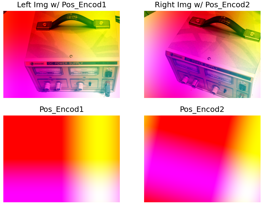
Figure 5: Illustration of 2D rectification position encoding. Color patterns indicate the values of positional encodings.

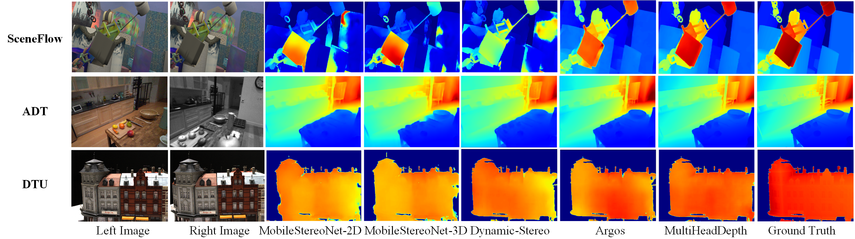
Figure 6: Output comparison cross models and datasets

Dataset	SceneFlow	ADT	DTU
Scenario	Synthetic scenarios (e.g. driving & flying items)	Ego-centric daily life scenarios	Robot arm rotating over a single item
Images Quality	Synthetic camera-based calibrated RGB images	Real camera-based RGB and Grayscale images	Real camera-based calibrated RGB images
Stereo Quality	Rectified	Rectified	Non-Rectified
Stereo Baseline	Static, 1.0 meter	Static, 12.8 cm	Dynamic, 7.8-14.9cm
Depth Map	Obtained by synthetic rendering	Obtained by twin digital synthetic rendering	Reconstructed from point clouds (need masks for invalid areas)

Table 1: Summary of Datasets

		MobileStereoNet-2D (WACV 2022 [24])			MobileStereoNet-3D (WACV 2022 [24])			Dynamic-Stereo (CVPR 2023 [11])			Argos (CVPR 2023 [28])			MultiheadDepth (Ours)
		AbsRel	D1	RMSE	AbsRel	D1	RMSE	AbsRel	D1	RMSE	AbsRel	D1	RMSE	AbsRel	D1	RMSE
Dataset	Sceneflow	0.172	0.71	8.2	0.129	0.42	5.9	0.287	0.89	68.8	0.102	0.23	5.3	0.091	0.35	4.3
	ADT	0.199	0.36	611.9	0.135	0.52	563.3	0.176	0.55	546.1	0.133	0.34	320.1	0.094	0.25	273.6
	DTU	0.147	0.38	315.9	0.148	0.40	224.8	0.339	0.88	628.5	0.122	0.61	536.9	0.101	0.42	216.1
Features	CPU Latency (ms)	4906.2			50313.7			1184.2			811.0			625.4
	GPU Latency (ms)	Out of Memory			Out of Memory			607.8			109.0			71.2
	FLOPS(G)	26.32			190.14			95.80			7.27			7.28
	#Params(M)	2.32			1.77			20.48			3.58			3.58

Table 2: The overall performance of the models. The datasets are used as inputs without any preprocessing. As indicated in Tab. 1, SceneFlow and ADT datasets consist of rectified stereo image inputs, while DTU contains unrectified stereo image inputs.

4.4 Structure of HomoDepth

Integrating our approaches discussed in  Sec. 4.2 and  Sec. 4.3 to MultiHeadDepth, we develop HomoDepth, which is illustrated in  Fig. 4. One key feature is the multi-task, which generates homography and depth estimation results using two heads connected to the encoder. Also, the RPE is integrated into the multi-head cost volume blocks and estimated homography matrix is used as an input to the multi-head cost volume block, as shown in Fig. 4.

In Fig. 4, we highlight training and inference flows using green and orange arrows, respectively. In the inference phase, the predicted homography matrix is passed to all the multi-head cost volumes, and the RPE is calculated inside it. The range of positional encoding is between 0 and 1, and it is added to the layer norm output. This ensures that the weights of input activations and positional encoding are balanced in the cost volume, allowing similarity to be assessed using both pattern and positional information.

During the training phase, the FC block and multi-head cost volume block are disconnected, resulting in two separate inputs and outputs in the model. The inputs include RGB stereo images and their homography matrix, while the outputs are the estimated homography and depth.

This structure is divided into three components: a common part (encoder), a depth estimation head, and a homography estimation head, as shown in Fig. 4. The shared encoder across two heads reduces overall computational costs and enables to perform two tasks with only a minor increase in latency for extra homography estimation head. However, training a multi-task model like this requires a specialized approach, which we discuss next.

4.5 Multi-task Model Training

To enable multi-task training of HomoDepth, we utilize the homoscedastic uncertainty [13] to train the model with the loss function adopted from Argos[28],

$$L_{D}(y,\hat{y}) =smooth\_L_{1}(y,\hat{y})$$ (6)

$$+\sum_{l=1}^{5}smooth\_L_{1}(grad(y^{l}),grad(\hat{y}^{l}))$$

where $smooth\_L_{1}$ is the SmoothL1Loss. $grad(y^{l})$ indicates the gradient of the depth map which is $2\times 2$ subsampled $l$ times. $y$ is the ground truth, and $\hat{y}$ is the prediction.

The loss function of homography estimation is formulated as follows:

$$L_{H}(y,\hat{y})=||weight_{w}(y)-weight_{w}(\hat{y})||_{F}$$ (7)

where

$$weight_{w}(y)=\begin{pmatrix}w&w&1\\ w&w&1\\ 1&1&w\end{pmatrix}\odot y$$ (8)

In the homography matrix, the first two rows and two columns represent the angular relationship between planes, usually with smaller values. The last column of the first two rows indicates the distance relationship between planes, generally with larger values. The $weight$ function applies weighting to smaller values by element-wise production, ensuring that all elements of the homography matrix are perceptible in the loss function, which is helpful with better homography matrix estimations. By default, we set $w$ as 50.

Utilizing the loss functions for homography and depth estimation. We formulate a unified total loss function as follows:

$$L=\frac{L_{H}}{2\sigma_{H}^{2}}+\frac{L_{D}}{2\sigma_{D}^{2}}+\log\sigma_{H}\sigma_{D}$$ (9)

where $\sigma_{H}$ and $\sigma_{D}$ represent homoscedastic uncertainties of two tasks. They are trainable parameters in HomoDepth.

5 Evaluation

We evaluate the effectiveness and efficiency of MultiHeadDepth and HomoDepth using three datasets on three platforms. We also show the quantization results of the models and discuss the robustness of HomoDepth.

5.1 Datasets

We utilize Scene Flow Dataset (SceneFlow) [19], DTU Robot Image Data Sets (DTU) [10], and Aria Digital Twin (ADT) [20] datasets to evaluate our models and a state-of-the-art stereo depth estimation model for AR glasses, Argos [28]. We summarize the characteristics of the datasets in Tab. 1.

SceneFlow SceneFlow is widely used for depth estimation tasks. However, the dataset contains rendered images from synthetic scenarios, which does not fully represent real-world scenarios. Also, its baseline is one meter, which is not aligned with that of AR glasses.

Aria Digital Twin (ADT) ADT consists of images captured by RGB and gray-scale fisheye cameras mounted on Aria AR glasses [5], a prototype AR glasses developed by Meta. Accordingly, the baseline and scenarios of the dataset are designed for AR applications. However, the ground truth depth in the dataset ignores human body in the images. To avoid disturbance from the property, we select 145 out of 236 scenarios that do not involve any human in the scene. Note that a scenario refers to a video that consists of many frames. We clarify details in Sec. 7.3.

ADT dataset provides one RGB image from the left and one gray-scale fisheye image from the right side for each scene due to the specification of the Aria glasses. Since both RGB and fisheye images are distorted, we apply calibration before feeding images to the models. Also, we replicate the calibrated grayscale images on channel dimension to match the shape of the RGB input tensor.

DTU Robot Image Data Sets (DTU) Dataset The DTU dataset is designed for multi-view stereo (MVS) reconstruction task. The dataset consists of images captured by a camera mounted on a robotic arm performing spherical scans, which move the robot arm from left to right with a slight downward tilt to the left back upon reaching the edge. We utilize images captured at neighboring positions as stereo image pairs for training. Compared to other MVS datasets, the DTU dataset is closer to the AR glasses scenarios for the following reasons: (1) Its scanning trajectory is close to the horizontal line, which can mimic the misalignment of stereo images. (2) The scanning intervals, or the baselines between adjacent images, are around 10 cm, which is similar to the cameras baseline on AR glasses.

We trained the models on each of these three datasets separately and compared the performance of the models. Specifically, since the DTU contains the extrinsic parameters of each frame, we leverage them in calculating the homography matrix over each stereo image inputs taken from two neighboring frames. We utilize the calculated homography matrix as the ground truth for the homography estimation in HomoDepth.

	AbsRel of Datasets			Latency (ms)
	SceneFlow	ADT	DTU	CPU	GPU
Argos (CVPR 2023)	0.109	0.146	0.140	748.5	54.4
MultiheadDepth (Ours)	0.098	0.097	0.112	598.9	45.3

Table 3: The performance of quantized models (INT8). The latencies are measured on a laptop with Intel® Core™ i7-12700H CPU and Nvidia® GeForce RTX 3070 Ti laptop GPU.

		Argos			PreP+Argos			PreP+MultiHeadDepth			HomoDepth
		AbsRel	D1	RMSE	AbsRel	D1	RMSE	AbsRel	D1	RMSE	AbsRel	D1	RMSE
Dataset	DTU	0.122	0.61	536.91	0.109	0.54	210.8	0.099	0.38	204.4	0.098	0.38	208.8
	DTU_df	0.183	0.64	599.32	0.115	0.55	223.1	0.107	0.48	287.8	0.087	0.32	184.9
Latency (ms)	CPU	811.0			1068.3			884.4			761.2
	GPU	109.0			312.5			312.6			84.5

Table 4: Ablation study comparing models with or without rectification preprocessing (PreP). DTU dataset represents a stereo system with a fixed focal length but variable relative position, while DTU_df represents a system with both variable focal length and position.

5.2 Implementation details

We implement MultiHeadDepth and HomoDepth in Pytorch [21] and train on Nvidia®  RTX 4090 32GB GPUs. We also run all the models involved in this section to obtain the test results. In experiment, we resize input images to $288\times 384\times 3$. The optimizer is Adam. In the early stages of model training, the base learning rate is 1e-4, and during the fine-tuning phase, it is adjusted to 4e-4.

5.3 Evaluation Metrics and Platform

We adopt AbsRel, D1, and RMSE as the evaluation metrics to measure model performance. All the metrics are ”Lower is Better” metrics, where smaller values represent higher model performance. We provide the detailed definition of each metric in Sec. 7.4.

Since our model’s eventual target is AR glasses, and we couldn’t find AR glasses with open API, we use three mobile platforms for latency evaluation as proxy. For the main model performance evaluation, we use a laptop with Intel® Core™ i7-12700H CPU and Nvidia® GeForce RTX 3070 Ti laptop GPU. We also measure the inference latency of our models on NVIDIA® Jetson Orin Nano™  Developer Kit [1] and a smartphone equipped with Snapdragon 8+ Gen 1 [2].

5.4 MultiHeadDepth Performance

We first evaluate the model performance on calibrated inputs. We compare the performance of MultiHeadDepth against four state-of-the-art stereo depth estimation models listed in Tab. 2. The results demonstrate that Argos and MultiHeadDepth are superior solutions for evaluated scenarios designed to model AR glasses. Comparing MultiHeadDepth against Argos, MultiHeadDepth provides 11.8-30.3% improvements in accuracy and 22.9-25.2% reduction in latency. The results show the effectiveness of our approach to optimize the cost volume blocks.

Impact of Quantization.

As quantization is commonly adopted optimization like Argos [28], we also evaluate quantized models and present the results in Tab. 3. In this study, we use AIMET [25] from Qualcomm to perform a post-training quantization. Although the overall accuracy decreases slightly by 3.1-14.7%, the latency is considerably reduced by 7.7-43.4% after quantization. MultiHeadDepth remains superior in all metrics after quantization.

5.5 HomoDepth Performance

In this session, we focus on the DTU scenarios that require preprocessing (rectification) and evaluate models with preprocessing and HomoDepth on such scenarios. We conduct the efficacy of RPE in the model through ablation studies of the end-to-end model (preprocessing + depth estimation). Utilizing the DTU dataset, we create a custom dataset, DTU_df, by scaling and cropping DTU images to simulate varying focal lengths, where ”df” stands for dynamic focal length. Thus, the DTU dataset represents a stereo system with a fixed focal length but variable relative position, while DTU_df represents a system with both variable focal length and relative position.

In Tab. 4 we evaluate four models with and without preprocessing. Although MultiHeadDepth achieves shorter inference latency, it still relies on preprocessing to achieve better accuracy, as compared in Tab. 2 and Tab. 4. In contrast, HomoDepth, despite having longer inference latency, does not require preprocessing. When the stereo cameras are misaligned, HomoDepth becomes a better solution. It not only delivers higher accuracy but also saves 30% of the total pipeline time.

5.6 Latency on Edge Devices

In this study, we report the latencies on two mobile/edge scale devices, NVIDIA® Jetson Orin Nano™  Developer Kit and Snapdragon 8+ Gen 1 Mobile Platform in Tab. 5. On the Orin Nano, the models are executed in eager mode. On the Snapdragon, the models are compiled using SNPE [22] and executed via ADB commands. The results may vary due to different deployment methods. We observe our models overall achieve better latency compared to Argos. Note that Argos results do not include preprocessing delay, while HomoDepth can accept unrectified data without preprocessing.

	Orin Nano		Snapdragon
	CPU	GPU	CPU	GPU
Argos (CVPR 2023)	8774	209	1424	914
MulHeadDepth (Ours)	6183	216	1156	617
HomoDepth (Ours)	6611	203	1512	893

Table 5: Latency of models in millisecond on NVIDIA® Jetson Orin Nano™  Developer Kit and Snapdragon 8+ Gen 1 Mobile Platform

6 Conclusion

Achieving both high model performance and low latency is a key toward depth estimation on AR glasses platforms. In this work, we identify preprocessing (rectification) and cost volume as the major optimization targets for low latency. By analyzing hardware-friendly and -unfriendly operations in existing cost volume, we develop an apporiximation of cosine similarity and employ a group-pointwise convolution that adopts the multi-head attention’s approach. For preprocessing, we introduce rectification positional encoding (RPE) and leverage homography matrix estimated by a head attached to the common encoder in our multi-head cost voulme blocks, which significantly reduces overall computational complexity.

Our approaches are complementary to any stereo depth estimation systems with online rectification and/or cost volume. In addition to the broad applicability, our evaluation results indicate our approaches are effective in improving model performance as well as achieving low latency. Therefore, we believe our work is making a meaningful step forward in the field of stereo depth estimation systems.

For one-shot scenarios, we recommend using HomoDepth. For continuous frames scenarios, we assume that the relative positions of the cameras on AR glasses remain stable over a short period. Therefore, we recommend first running HomoDepth to obtain depth estimation while simultaneously deriving the homography between the two cameras. For subsequent stereo inputs, homography rectification can be quickly applied, and MultiHeadDepth can be utilized to achieve higher efficiency.

7 Appendix

7.1 Computational Complexity of Multi-head Cost Volume

Suppose the dimension of an input activation is $CHW$, and the max disparity is $d$. The number of multiply-accumulate operations (#MAC) of the original cost volume is $3CHWd$ (please refer to Algorithm 1). The layer norm along channel dimension is defined as Eq. 10, whose #MAC is $3HWd$. Replacing the cosine similarity with the dot product, and add the layer norm before the loop. The #MAC of multi-head cost volume is $2\times 3CHW+CHWd<3CHWd$.

$$y=\frac{x-E[x]}{\sqrt{Var[x]+\epsilon}}\gamma+\beta$$ (10)

7.2 SIFT v.s. Conv Network

As [27] analyses, the computational complexity of SIFT for an $N\times N$ image with $n\times n$ tiles is

$$\Theta\left(\frac{(n+x)^{2}}{p_{i}\,\Gamma_{0}}+\alpha\beta N^{2}x^{2}\Gamma_{1}+\frac{(\alpha\beta+\gamma)n^{2}\log x}{p_{o}\,\Gamma_{2}}\right)$$ (11)

where x is the neighborhood of tiles. $N\gg n>x$ in most cases, we can simplify the complexity as $O(N^{2})$.

For convolutional networks, the computational complexity for an $N\times N$ input activation with $C$ channels in input and $C`$ channels in output is,

$$O(N^{2}CC^{\prime}k^{2})$$ (12)

where $k$ is the convolution kernel size. $N\gg C>k$ in most cases, we can also simplify the complexity as $O(N^{2})$.

Based on the above analysis, we can conclude that: Supervised learning convolutional neural networks capable of the same task will not perform worse efficiency for all computer vision algorithms requiring key point matching. As the same, CNN is not worse than the classic algorithm in homography estimation tasks.

In practice, many optimizations for CNNs have been proposed, and CNN computations are more hardware-friendly. In contrast, [27] has been proven that without improvements in the input bandwidth, the power of multicore processing cannot be used efficiently for SIFT. Therefore, CNNs are generally a more efficient approach. Based on the report in [28] and our experiments, keypoint matching takes around 300ms on both smartphones and laptops. There is no significant speed up from smartphone to laptop, showing the limitations of keypoint matching.

7.3 Dataset Setting

DTU setting:

Based on previous implementations and common practices [29], we selected the evaluation set as scans {1, 4, 9, 10, 11, 12, 13, 15, 23, 24, 29, 32, 33, 34, 48, 49, 62, 75, 77, 110, 114, 118}, validation set: scans {3, 5, 17, 21, 28, 35, 37, 38, 40, 43, 56, 59, 66, 67, 82, 86, 106, 117}, and the rest is training set.

Additionally, our network takes two images as input, but the depth map is aligned with the left image. This means that the left and right inputs cannot be interchanged. We need to match the stereo images to ensure that the relative position of the left input is indeed on the left side of the right input. The image match list is shown as Tab. 6.

ADT setting:

As mentioned, ATD ignores users’ bodies in the images when rendering ground truth depth maps which causes inconsistencies between the input images and the predicted results. We selected subsets of the scene where no other users were present. The selected subset can be obtained by this query link: https://explorer.projectaria.com/adt?q=%22is_multi_person+%3D%3D+false%22

L	1	2	3	4	5	7	8	9	10	11	12	12
R	2	3	4	5	6	6	7	8	9	10	11	13
L	13	14	15	16	17	18	19	21	22	23	24	25
R	14	15	16	17	18	19	20	20	21	22	23	24
L	26	27	28	29	29	30	31	32	33	34	35	36
R	25	26	27	28	30	31	32	33	34	35	36	37
L	38	40	41	42	43	44	45	45	46	47	48	49
R	39	39	40	41	42	43	44	44	45	46	47	48

Table 6: Input images pairs of DTU Dataset

7.4 Metrics Definition

Here are the definitions of the metrics we used for evaluation:

$$AbsRel =\frac{1}{N}\sum_{i=1}^{N}\frac{\hat{y}_{i}-y_{i}}{y_{i}}$$ (13)

$$D1 =\frac{1}{N}\sum_{i=1}^{N}\mathbf{1}(\frac{|\hat{y}_{i}-y_{i}|}{y_{i}}\leq 5\%)$$ (14)

$$RMSE =\sqrt{\frac{1}{N}\sum_{i=1}^{N}(\hat{y}_{i}-y_{i})^{2}}$$ (15)

where $N$ is the total number of pixels of the depth maps, $y_{i}$ is the value of pixels in ground truth map, and $\hat{y_{i}}$ is the value of pixels in prediction.

7.5 Robustness Analysis

HomoDepth is a muti-task learning structure, and the depth estimation depends on the predicted homography matrix. Thus, the accuracy of homography estimation affects depth estimation. In this section, we address two questions: (1) How sensitive is the depth estimation to the homography estimation? (2) How stable is the homography estimation?

Homography Estimation Errors.

We analyze the error of HomoDepth during homography estimation. In practice, the error variance is as small as 0.003, as shown in Fig. 7(a). This indicates that the homography estimation of HomoDepth is highly accurate.

Sensitivity Study.

In HomoDepth, we inject noise $n\sim N(0,\sigma)$, where $\sigma\in[0,2]$, to the elements of estimated homography matrix before it is passed to the multi-head cost volume blocks. Then, we investigate the final depth estimation errors. The instability is quantified by examining the noise variance and corresponding changes in the smooth loss function Eq. 6 corresponding to depth estimation. As shown in Fig. 7(b), the standard deviation trends indicate that depth estimation remains stable when $\sigma<0.5$. The linear fitting demonstrates that the loss values increase as the noise variance grows.

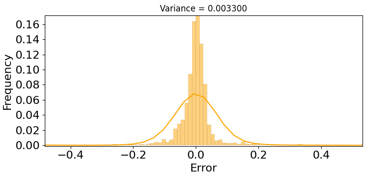
(a) The statistics of the error in homography estimation. The curve represents the Gaussian fitting of the statistical results.

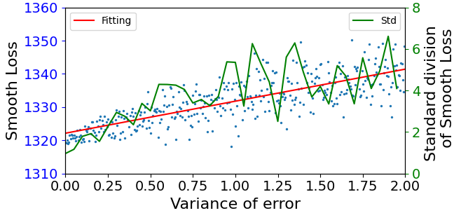
(b) The simulation of the influence of noise added to the homography matrix. The blue scatter points represent the average loss values corresponding to noise variances $\sigma$. The green lines indicate the standard deviation of the loss values for noise variance $\sigma$. The red line represents the linear fitting of the blue scatter points, showing the trend of loss with increasing noise variance.

Figure 7: The robustness analyze of HomoDepth

References

- [1] Jetson orin nano developer kit getting started guide. https://developer.nvidia.com/embedded/learn/get-started-jetson-orin-nano-devkit. Accessed on Nov 12, 2024.
- [2] Snapdragon 8+ gen 1 mobile platform. https://www.qualcomm.com/products/mobile/snapdragon/smartphones/snapdragon-8-series-mobile-platforms. Accessed on Nov 12, 2024.
- Ahn et al. [2019] Jong-gil Ahn, Euijai Ahn, Seulki Min, Hyeonah Choi, Howon Kim, and Gerard J. Kim. Size perception of augmented objects by different ar displays. In HCI International 2019 - Posters, pages 337–344, Cham, 2019. Springer International Publishing.
- DeTone et al. [2016] Daniel DeTone, Tomasz Malisiewicz, and Andrew Rabinovich. Deep image homography estimation, 2016.
- et al. [2023] Jakob Engel et al. Project aria: A new tool for egocentric multi-modal ai research, 2023.
- Faugeras [1993] Olivier Faugeras. Three-dimensional computer vision: a geometric viewpoint. MIT press, 1993.
- Gan et al. [2021] Wanshui Gan, Pak Kin Wong, Guokuan Yu, Rongchen Zhao, and Chi Man Vong. Light-weight network for real-time adaptive stereo depth estimation. Neurocomputing, 441:118–127, 2021.
- Hartley and Zisserman [2003] Richard Hartley and Andrew Zisserman. Multiple View Geometry in Computer Vision. Cambridge University Press, New York, NY, USA, 2 edition, 2003.
- Hirschmuller and Scharstein [2007] Heiko Hirschmuller and Daniel Scharstein. Evaluation of cost functions for stereo matching. In 2007 IEEE Conference on Computer Vision and Pattern Recognition, pages 1–8, 2007.
- Jensen et al. [2014] Rasmus Jensen, Anders Dahl, George Vogiatzis, Engil Tola, and Henrik Aanæs. Large scale multi-view stereopsis evaluation. In 2014 IEEE Conference on Computer Vision and Pattern Recognition, pages 406–413. IEEE, 2014.
- Karaev et al. [2023] Nikita Karaev, Ignacio Rocco, Benjamin Graham, Natalia Neverova, Andrea Vedaldi, and Christian Rupprecht. Dynamicstereo: Consistent dynamic depth from stereo videos, 2023.
- Kendall et al. [2017] Alex Kendall, Hayk Martirosyan, Saumitro Dasgupta, Peter Henry, Ryan Kennedy, Abraham Bachrach, and Adam Bry. End-to-end learning of geometry and context for deep stereo regression. In Proceedings of the IEEE International Conference on Computer Vision (ICCV), 2017.
- Kendall et al. [2018] Alex Kendall, Yarin Gal, and Roberto Cipolla. Multi-task learning using uncertainty to weigh losses for scene geometry and semantics, 2018.
- Kopf et al. [2020] Johannes Kopf, Kevin Matzen, Suhib Alsisan, Ocean Quigley, Francis Ge, Yangming Chong, Josh Patterson, Jan-Michael Frahm, Shu Wu, Matthew Yu, Peizhao Zhang, Zijian He, Peter Vajda, Ayush Saraf, and Michael Cohen. One shot 3d photography, 2020.
- Kumar et al. [2010] Sanjeev Kumar, Christian Micheloni, Claudio Piciarelli, and Gian Luca Foresti. Stereo rectification of uncalibrated and heterogeneous images. Pattern Recognit. Lett., 31:1445–1452, 2010.
- Kwon et al. [2023] Hyoukjun Kwon, Krishnakumar Nair, Jamin Seo, Jason Yik, Debabrata Mohapatra, Dongyuan Zhan, Jinook Song, Peter Capak, Peizhao Zhang, Peter Vajda, et al. Xrbench: An extended reality (xr) machine learning benchmark suite for the metaverse. Proceedings of Machine Learning and Systems, 5, 2023.
- Li et al. [2021] Mengdi Li, Cornelius Weber, Matthias Kerzel, Jae Hee Lee, Zheni Zeng, Zhiyuan Liu, and Stefan Wermter. Robotic occlusion reasoning for efficient object existence prediction, 2021.
- Lutwak et al. [2023] Hope Lutwak, T. Scott Murdison, and Kevin W. Rio. User Self-Motion Modulates the Perceptibility of Jitter for World-locked Objects in Augmented Reality . In 2023 IEEE International Symposium on Mixed and Augmented Reality (ISMAR), pages 346–355, 2023.
- Mayer et al. [2016] N. Mayer, E. Ilg, P. Häusser, P. Fischer, D. Cremers, A. Dosovitskiy, and T. Brox. A large dataset to train convolutional networks for disparity, optical flow, and scene flow estimation. In IEEE International Conference on Computer Vision and Pattern Recognition (CVPR), 2016. arXiv:1512.02134.
- Pan et al. [2023] Xiaqing Pan, Nicholas Charron, Yongqian Yang, Scott Peters, Thomas Whelan, Chen Kong, Omkar Parkhi, Richard Newcombe, and Yuheng (Carl) Ren. Aria digital twin: A new benchmark dataset for egocentric 3d machine perception. In Proceedings of the IEEE/CVF International Conference on Computer Vision (ICCV), pages 20133–20143, 2023.
- Paszke et al. [2019] Adam Paszke, Sam Gross, Francisco Massa, Adam Lerer, James Bradbury, Gregory Chanan, Trevor Killeen, Zeming Lin, Natalia Gimelshein, Luca Antiga, Alban Desmaison, Andreas Köpf, Edward Yang, Zach DeVito, Martin Raison, Alykhan Tejani, Sasank Chilamkurthy, Benoit Steiner, Lu Fang, Junjie Bai, and Soumith Chintala. PyTorch: an imperative style, high-performance deep learning library. Curran Associates Inc., Red Hook, NY, USA, 2019.
- Qualcomm Technologies [2024] Inc. Qualcomm Technologies. Snapdragon Neural Processing Engine (SNPE) Developer Guide, 2024.
- Sandler et al. [2019] Mark Sandler, Andrew Howard, Menglong Zhu, Andrey Zhmoginov, and Liang-Chieh Chen. Mobilenetv2: Inverted residuals and linear bottlenecks, 2019.
- Shamsafar et al. [2021] Faranak Shamsafar, Samuel Woerz, Rafia Rahim, and Andreas Zell. Mobilestereonet: Towards lightweight deep networks for stereo matching, 2021.
- Siddegowda et al. [2022] Sangeetha Siddegowda, Marios Fournarakis, Markus Nagel, Tijmen Blankevoort, Chirag Patel, and Abhijit Khobare. Neural network quantization with ai model efficiency toolkit (aimet), 2022.
- Vaswani et al. [2023] Ashish Vaswani, Noam Shazeer, Niki Parmar, Jakob Uszkoreit, Llion Jones, Aidan N. Gomez, Lukasz Kaiser, and Illia Polosukhin. Attention is all you need, 2023.
- Vinukonda [2011] Phaneendra Vinukonda. A study of the scale-invariant feature transform on a parallel pipeline. Master’s thesis, Louisiana State University, 2011. LSU Master’s Theses, 2721.
- Wang et al. [2023] Jialiang Wang, Daniel Scharstein, Akash Bapat, Kevin Blackburn-Matzen, Matthew Yu, Jonathan Lehman, Suhib Alsisan, Yanghan Wang, Sam Tsai, Jan-Michael Frahm, et al. A practical stereo depth system for smart glasses. In Proceedings of the IEEE/CVF Conference on Computer Vision and Pattern Recognition, pages 21498–21507, 2023.
- Yao et al. [2018] Yao Yao, Zixin Luo, Shiwei Li, Tian Fang, and Long Quan. Mvsnet: Depth inference for unstructured multi-view stereo, 2018.
- Zhang et al. [2022] Jinrui Zhang, Huan Yang, Ju Ren, Deyu Zhang, Bangwen He, Ting Cao, Yuanchun Li, Yaoxue Zhang, and Yunxin Liu. Mobidepth: real-time depth estimation using on-device dual cameras. In Proceedings of the 28th Annual International Conference on Mobile Computing And Networking, page 528–541, New York, NY, USA, 2022. Association for Computing Machinery.