Photon polarization tensor at finite temperature and density in a magnetic field

Abstract

We present analytical and numerical calculations for the photon polarization tensor at finite temperature and density in a constant magnetic field. We first discuss the tensor decomposition in the presence of the magnetic field which breaks rotational symmetry. Then, we analytically perform all the momentum integrations and numerically take the Landau level sum. We present the real and imaginary parts of the photon polarization tensor as functions of the momenta, the chemical potential, and the finite temperature. As an application, we consider the real photon limit and estimate the photon decay rate in the hot and dense medium. We specifically quantify the difference between the X-mode and the O-mode with the polarization orthogonal and parallel to the magnetic field. As long as the magnetic field is weak, the decay rate of the X-mode photon is larger than that of the O-mode photon, while the O-mode becomes dominant due to the Landau level suppression of the X-mode at strong magnetic field.

1 Introduction

Both theoretically and phenomenologically, magnetic fields are important probes across a wide range of fields in physics, including condensed matter physics, astrophysics, and nuclear physics. Physics in quantum chromodynamics (QCD) is rich and complicated, and various aspects in QCD have been revealed with magnetic field probes. To give some examples, theoretical investigations on the QCD phase diagram in the presence of an external magnetic field $B$ have been addressed Fraga:2008qn ; Mizher:2010zb ; Ferrer:2013noa ; Gatto:2010qs ; Gatto:2010pt ; Ferreira:2014kpa ; Mueller:2015fka , and enhancement of chiral symmetry breaking by magnetic fields is known as the magnetic catalysis and has been discussed over decades Klimenko:1991he ; Gusynin:1994re ; Gusynin:1995nb ; Shushpanov:1997sf ; Fukushima:2012xw ; Bali:2013txa ; see ref. Miransky:2015ava for a review. Besides, the Monte-Carlo simulation in QCD with external magnetic fields has been conducted without the sign problem DElia:2010abb ; Bali:2011qj ; see ref. Endrodi:2024cqn for the state-of-the-art overview. The simulation has provided us with deep insights into QCD phenomena induced by the magnetic fields; the inverse magnetic catalysis was discovered in lattice QCD at high temperaute Bali:2011qj ; Bali:2012zg ; Bruckmann:2013oba , the meson mass spectra under magnetic background invoked inspiring discussions on the physical interpretation Hidaka:2012mz ; Hattori:2015aki ; Ding:2020jui , and so on.

The phenomenological aspects of magnetic fields have attracted a lot of attention, especially in the theoretical community, on demand from real experiments. Indeed, in non-central heavy-ion collisions at Relativistic Heavy Ion Collider (RHIC) and Large Hadron Collider (LHC), strong magnetic fields $\sim 10^{18}$ G (comparable to $m_{\pi}^{2}$) should be realized Skokov:2009qp ; Voronyuk:2011jd ; Deng:2012pc ; McLerran:2013hla . Since the energy scales of $B$ and the temperature $T$ are larger than the light-flavor quark mass, a quark-gluon plasma (QGP) can be regarded as a chiral material that exhibits nontrivial phenomena. For example, several anomalous transport effects as represented by the chiral magnetic effect Kharzeev:2007jp ; Fukushima:2008xe , the chiral separation effect Son:2004tq ; Metlitski:2005pr , and the chiral vortical effect Son:2009tf ; Kharzeev:2010gr are believed to emerge from properties of the chiral materials Kharzeev:2004ey ; Kharzeev:2007jp ; Kharzeev:2013ffa ; Shi:2017cpu ; see ref. Kharzeev:2015znc for a review. Importantly, these effects are attributed to macroscopic manifestations of the chiral anomaly and QCD topological structures. It should be noted that the large vorticity, an analogue of the magnetic field, has been confirmed experimentally by hyperon global polarization measured by the STAR collaboration at RHIC STAR:2017ckg as predicted by the theoretical work Liang:2004ph . The estimate of vorticity assumes a formula derived in ref. Becattini:2016gvu in which the magnetic effect of the intrinsic magnetic moments of created particles was also discussed.

It would be of great significance to investigate magnetized QCD matter not only along the temperature axis. Cold and dense quark matter such as a color superconductor with strong magnetic fields might be realized in cores of neutron stars Alford:1999pb ; Ferrer:2005vd ; Ferrer:2006vw ; Noronha:2007wg ; Fukushima:2007fc . The strength of magnetic fields at the surface of specific neutron stars called magnetars is estimated to be of order $10^{15}$ G. Since the magnetic flux in the central cores of the stars is squeezed, the field strength is thought to be as high as $\sim 10^{18}$ G. It is conceivable that such strong $B$ affects the ground state properties in QCD matter. One plausible candidate of the true ground state is the chiral soliton lattice, which turns out to be energetically favored at high density and strong magnetic field Brauner:2016pko ; Chen:2021vou ; Qiu:2023guy ; Evans:2023hms .

In addition, the magnetic fields on magnetar surfaces have drawn increasing attention in recent years. This is caused by the possibility that we can estimate the strength and geometry of the magnetars’ magnetic fields through the X-ray polarization observation from the Imaging X-ray Polarimetry Explorer (IXPE) Taverna:2020vpr ; Taverna:2022jgl ; Taverna:2024uop . In general, photons under strong magnetic fields have two distinct modes with linear polarizations; namely, the ordinary mode (O-mode) with polarization parallel to the magnetic field and the extraordinary mode (X-mode) with polarization perpendicular to the magnetic field. From the observational data from IXPE, the polarization angle and polarization degree of X-ray have been extracted as functions of the energy of photons. With this extracted information, we could reconstruct the profile of the magnetic fields of magnetars. Indeed, some models are proposed to explain the observational data. For example, in the resonance Compton scattering scenario Taverna:2022jgl , the cross section of the Compton scattering between photons and electrons becomes large when the energy of photons is comparable to the cyclotron frequency of electrons. As a result, the resonant cross section is mode-sensitive and this scenario yields the polarization degree $\sim 33\%$ of X-rays from the magnetosphere. However, according to the IXPE results Taverna:2022jgl ; Zane:2023khc ; Turolla:2023ruu , the polarization degree reaches as large as $80\%$ and energy dependence of the polarization degree was found to be sizable. It is further puzzling that the polarization angle swings by $90\mathrm{°}$ as the energy of photons changes. To make a consistent view, the mode conversion scenario was discussed in refs. Lai:2003nd ; Lai:2022knd . In this scenario, the combination of the vacuum birefringence effects and the plasma birefringence effects results in a stochastic conversion of the O-mode into the X-mode of photons, and vice versa. Although this scenario can successfully explain the observation qualitatively, it is desirable to improve it to make a quantitative match with the data. In order to supplement this model with electron contribution corrections, the field-theoretical evaluation of the polarization tensor with electron loops is necessary. To this end, we calculate the polarization tensor in the framework of quantum field theory at finite temperature and density.

As mentioned above, there are so many physical systems where the magnetic fields play an important role, which has motivated a lot of theoretical works involving magnetic fields. In particular, the field-theoretical calculation in the presence of external electromagnetic fields was founded by Schwinger, which can be traced back to the old days of Euler and Heisenberg. They suggested that the QED vacuum filled with electrons and positrons is modified by the polarization with strong electromagnetic fields Heisenberg:1936nmg ; Schwinger:1951nm ; Dunne:2004nc ; Ferrer:2012pb . More recently, the vacuum contribution of the polarization tensor in magnetic fields was intensively discussed in refs. Baier:2007dw ; Hattori:2012je ; Hattori:2012ny . For the finite temperature, $T\neq 0$, and zero chemical potential, $\mu=0$, the strong field approximation for the polarization tensor was argued in ref. Alexandre:2000jc , and the full Landau level calculation for the imaginary part of the polarization tensor is found in refs. Wang:2020dsr ; Wang:2021ebh , which has been extended to finite density, $\mu\neq 0$ Wang:2021eud . The calculation would become simple in the lowest Landau level approximation as argued in refs. Hattori:2022uzp ; Hattori:2022wao . In addition, for $T\neq 0$ and $\mu\neq 0$, the dynamical polarization function of graphene in a magnetic field was treated in ref. Pyatkovskiy:2010xz . The relation between the eigenmodes of propagating photons and the polarization tensor in a magnetic field for $T\neq 0$ and $\mu\neq 0$ was discussed in PerezRojas:1979jrk . The present work aims to complete the full analysis of the real part of the polarization tensor as well as the imaginary part at finite $T$ and $\mu$ taking account of all Landau levels.

2 Formulation

This paper aims to complete the full evaluation of the photon polarization tensor with electrons and positrons at finite temperature and density. We will proceed to the technical details of the explicit derivation in the next section. Here, we shall summarize basic formulas that would be convenient for clarifying our convention.

2.1 Propagator in the magnetic field

The electron field, $\psi(x)$, satisfies the following Dirac equation:

$$(\mathrm{i}\not{D}-m)\psi(x)=0\,,$$ (1)

where $m$ is the electron mass and $\not{D}\coloneqq\gamma^{\mu}D_{\mu}$ is Feynman’s slash. The Dirac matrices, $\gamma^{\mu}$, satisfy the Clifford algebra, $\{\gamma^{\mu},\gamma^{\nu}\}=2\eta^{\mu\nu}$, where $\eta_{\mu\nu}=\mathop{\mathrm{diag}}(1,-1,-1,-1)$ in our convention. The covariant derivative for the electron is $D_{\mu}\coloneqq\partial_{\mu}-\mathrm{i}eA_{\mu}$ with $e>0$, i.e., the electron charge is $-e$. We choose the $z$-axis along the external magnetic field direction; $\bm{B}=(0,0,B)$ with $B>0$. Throughout this paper, we will work in a symmetric gauge, $A^{\mu}=(0,-yB/2,xB/2,0)$. In our notation, we write the four-momentum simply as $p^{\mu}=(p_{0},p_{x},p_{y},p_{z})$ using the coordinate subscripts and define the transverse and the longitudinal four momenta as $p^{\mu}_{\perp}=(0,p_{x},p_{y},0)$ and $p^{\mu}_{\parallel}=(p_{0},0,0,p_{z})$, respectively. We note that $p_{\perp}^{2}=-p_{x}^{2}-p_{y}^{2}=-{\bm{p}}_{\perp}^{2}$ and $p_{\parallel}^{2}=p_{0}^{2}-p_{z}^{2}$. In the imaginary-time formalism of quantum field theory at finite temperature $T$ and chemical potential $\mu$, we may replace $p^{\mu}\to\tilde{p}^{\mu}\coloneqq(\mathrm{i}\nu_{n}+\mu,{\bm{p}})$ with the fermionic Matsubara frequency given by $\nu_{n}=(2n+1)\pi T$ ($n\in\mathbb{Z}$). Then, the electron propagator in the imaginary-time formalism reads:

$$S(\tilde{p})=\sum_{l=0}^{\infty}\frac{-S_{l}(\tilde{p})}{\tilde{p}_{\parallel}^{2}-m_{l}^{2}}\,.$$ (2)

We note that the Schwinger phase is dropped because it is irrelevant in calculating the polarization tensor. In the denominator $m_{l}^{2}\coloneqq 2eBl+m^{2}$ is the effective transverse mass at the Landau level $l$. The numerator on the right-hand side is

$$S_{l}(p)\coloneqq(\not{p}_{\parallel}+m)\bigl{[}P_{-}A_{l-}(\xi_{p})+P_{+}A_{l+}(\xi_{p})\bigr{]}+\not{p}_{\perp}B_{l}(\xi_{p})\,,$$ (3)

where we define the following functions:

$$A_{l-}(\xi_{p}) \coloneqq 2\mathrm{e}^{-2\xi_{p}}(-1)^{l}L_{l}(4\xi_{p})\,,$$ (4a)

$$A_{l+}(\xi_{p}) \coloneqq 2\mathrm{e}^{-2\xi_{p}}(-1)^{l-1}L_{l-1}(4\xi_{p})\,,$$ (4b)

$$B_{l}(\xi_{p}) \coloneqq 4\mathrm{e}^{-2\xi_{p}}(-1)^{l-1}L_{l-1}^{(1)}(4\xi_{p})\,,$$ (4c)

where a dimensionless variable, $\xi_{p}\coloneqq\bm{p}^{2}_{\perp}/(2eB)$, is introduced for notational brevity. In this work, we adopt the following definition for the generalized Laguerre polynomials:

$$L_{n}^{(\alpha)}(x)\coloneqq\frac{\mathrm{e}^{x}x^{-\alpha}}{n!}\derivative[n]{x}\mathrm{e}^{-x}x^{n+\alpha}$$ (5)

and the Laguerre polynomials are $L_{n}(x)=L_{n}^{(0)}(x)$ in particular. In our present convention, $L_{-n}^{(\alpha)}(x)=0$ for $n>0$ should be understood. It is thus evident from eq. (3) that the Landau zero mode exists only for one spin state projected by $P_{-}$. The quantity inside the square brackets contains the projection operators of the spin along the $z$-axis (for $eB>0$):

$$P_{\pm}\coloneqq\frac{1}{2}\bigl{(}1\pm\mathrm{i}\gamma^{1}\gamma^{2}\bigr{)}\,.$$ (6)

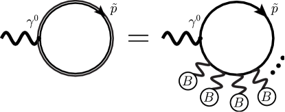
Figure 1: Tadpole diagram for calculating the expectation value of the density.

Before dealing with the polarization tensor which has 16 components, let us consider the calculation of the density, $\langle n(x)\rangle=\langle\bar{\psi}(x)\gamma^{0}\psi(x)\rangle$, as a one-component warm-up exercise. Figure 1 shows the diagram corresponding to $\langle n(x)\rangle$. We use the double line to represent the fermion propagator in the presence of background $\bm{B}$ as schematically illustrated in figure 1. Due to translational symmetry, we can take $x=0$ to simplify the expression slightly as

$$\langle n(0)\rangle=(-1)T\!\!\sum_{n=-\infty}^{\infty}\sum_{l=0}^{\infty}\int\frac{\differential[3]{p}}{(2\pi)^{3}}\frac{-\tr[\gamma^{0}S_{l}(\tilde{p})\bigr{]}}{\tilde{p}_{\parallel}^{2}-m_{l}^{2}}\,.$$ (7)

The overall minus sign appears from the fermion loop. Then, it is straightforward to take the trace using eq. (3) to find

$$\langle n(0)\rangle =\sum_{l=0}^{\infty}\int\frac{\differential[2]{p_{\perp}}}{(2\pi)^{2}}\,\mathrm{e}^{-2\xi_{p}}(-1)^{l}\Bigl{[}L_{l}(4\xi_{p})-L_{l-1}(4\xi_{p})\Bigr{]}T\!\!\sum_{n=-\infty}^{\infty}\int\frac{\differential{p_{z}}}{2\pi}\frac{4\tilde{p}^{0}}{\tilde{p}_{\parallel}^{2}-m_{l}^{2}}$$

$$=\frac{eB}{8\pi}\sum_{l=0}^{\infty}\int_{0}^{\infty}\differential{u}\,\mathrm{e}^{-u/2}(-1)^{l}\Bigl{[}L_{l}(u)-L_{l-1}(u)\Bigr{]}\times$$

$$\qquad\qquad\qquad\qquad\times\int_{-\infty}^{\infty}\frac{\differential{p_{z}}}{2\pi}\,2\Bigl{[}n_{\mathrm{F}}(E_{l}(p_{z})-\mu)-n_{\mathrm{F}}(E_{l}(p_{z})+\mu)\Bigr{]}$$

$$=\frac{eB}{2\pi}\sum_{l=0}^{\infty}\alpha_{l}\int_{-\infty}^{\infty}\frac{\differential{p_{z}}}{2\pi}\Bigl{[}n_{\mathrm{F}}(E_{l}(p_{z})-\mu)-n_{\mathrm{F}}(E_{l}(p_{z})+\mu)\Bigr{]}\,,$$ (8)

where $E_{l}(p_{z})\coloneqq\sqrt{p_{z}^{2}+m_{l}^{2}}$ is the electron energy at the Landau level $l$. From the first to the second line, $u=4\xi_{p}$ is introduced, so that we can use the formula: $\int_{0}^{\infty}\differential{u}\,\mathrm{e}^{-u/2}L_{l}(u)=2(-1)^{l}$. The Matsubara sum leads to $n_{\mathrm{F}}$ that is the Fermi-Dirac distribution function:

$$n_{\mathrm{F}}(E)\coloneqq\frac{1}{\mathrm{e}^{E/T}+1}\,.$$ (9)

In the last line $\alpha_{l}$ represents the spin degeneracy factor, i.e., $\alpha_{0}=1$ and $\alpha_{l>0}=2$. We can easily check that the above expression for $\langle n(0)\rangle$ is reduced to the standard expression in the limit of vanishing $B$.

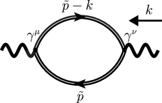
Figure 2: One-loop diagram for the photon polarization tensor.

2.2 One-loop polarization tensor

It is an immediate extension to apply the above technique to the polarization diagram at the one-loop level as depicted in figure 2. For the external momentum, $k^{\mu}=(\mathrm{i}\omega_{n},\bm{k})$ with $\omega_{n}=2n\pi T$ the bosonic Matsubara frequency, the polarization tensor reads:

$$\Pi^{\mu\nu}(\mathrm{i}\omega_{n},\bm{k})=(-1)e^{2}T\sum_{m=-\infty}^{\infty}\sum_{k,l=0}^{\infty}\int\frac{\differential[3]{p}}{(2\pi)^{3}}\frac{\tr[\gamma^{\mu}S_{k}(\tilde{p})\gamma^{\nu}S_{l}(\tilde{p}-{k})\bigr{]}}{(\tilde{p}_{\parallel}^{2}-m_{k}^{2})[(\tilde{p}_{\parallel}-{k}_{\parallel})^{2}-m_{l}^{2}]}\,.$$ (10)

Here again, the overall $(-1)$ appears from the fermion loop. We note $\tilde{p}_{0}=\mathrm{i}\nu_{m}+\mu$, where $\nu_{m}=(2m+1)\pi$ is the fermionic Matsubara frequency (not to be confused with the mass $m$). For notational simplicity, we represent the numerator by the following symbol,

$$h_{kl}^{\mu\nu}(p,k)\coloneqq\tr[\gamma^{\mu}S_{k}(p)\gamma^{\nu}S_{l}(p-k)]\,.$$ (11)

Since the denominator does not depend on transverse $p_{\perp}^{\mu}$, we can factorize the momentum integral as

$$\Pi^{\mu\nu}(\mathrm{i}\omega_{n},\bm{k})=(-1)e^{2}T\sum_{m=-\infty}^{\infty}\sum_{k,l=0}^{\infty}\int\frac{\differential{p_{z}}}{2\pi}\frac{H_{kl}^{\mu\nu}(\tilde{p}_{0},p_{z};k_{\parallel},z)}{(\tilde{p}_{\parallel}^{2}-m_{k}^{2})[(\tilde{p}_{\parallel}-{k}_{\parallel})^{2}-m_{l}^{2}]}\,,$$ (12)

where we define the numerator, i.e., the lepton tensor integral, as

$$H_{kl}^{\mu\nu}(\tilde{p}_{0},p_{z};k_{\parallel},z)\coloneqq\int\frac{\differential[2]{p_{\perp}}}{(2\pi)^{2}}\,h_{kl}^{\mu\nu}(\tilde{p},k)\,,$$ (13)

where $z\coloneqq\bm{k}_{\perp}^{2}/(2eB)$.

In later discussions, we shall evaluate $H_{kl}^{\mu\nu}(\tilde{p}_{0},p_{z};k_{\parallel},z)$, which is the central part in this paper, and for the moment, let us take the Matsubara sums. The standard technique leads to the following useful formula,

$$T\sum_{m=-\infty}^{\infty}\frac{g(\mathrm{i}\nu_{m}+\mu)}{[(\mathrm{i}\nu_{m}+\mu)^{2}-E_{1}^{2}][(\mathrm{i}\nu_{m}+\mu-\mathrm{i}\omega_{n})^{2}-E_{2}^{2}]}$$

$$=-\sum_{s_{1},s_{2}=\pm 1}\frac{s_{1}s_{2}}{4E_{1}E_{2}}\frac{1}{-\mathrm{i}\omega_{n}+s_{1}E_{1}-s_{2}E_{2}}\times$$

$$\qquad\qquad\times\Big{[}n_{\mathrm{F}}(\mu-s_{1}E_{1})g(s_{1}E_{1})-n_{\mathrm{F}}(\mu-s_{2}E_{2})g(s_{2}E_{2}+\mathrm{i}\omega_{n})\Bigr{]}\,.$$ (14)

Here $g(\mathrm{i}\nu_{m}+\mu)$ is an arbitrary function satisfying $\lim_{z\to\infty}|g(z)|<|z|^{3}$. Using this, we can simplify the polarization tensor in the following form:

$$\begin{split}&\Pi^{\mu\nu}(\mathrm{i}\omega_{n},\bm{k})\\ &=\sum_{k,l=0}^{\infty}\sum_{s_{1},s_{2}=\pm 1}e^{2}\int\frac{\differential{p_{z}}}{2\pi}\frac{s_{1}s_{2}}{4E_{k}E_{l}}\frac{1}{-\mathrm{i}\omega_{n}+s_{1}E_{k}-s_{2}E_{l}}\times\\ &\quad\times\Bigl{[}n_{\mathrm{F}}(\mu-s_{1}E_{k})H_{kl}^{\mu\nu}(s_{1}E_{k},p_{z};k_{\parallel},z)-n_{\mathrm{F}}(\mu-s_{2}E_{l})H_{kl}^{\mu\nu}(s_{2}E_{l}+\mathrm{i}\omega_{n},p_{z};k_{\parallel},z)\Bigr{]}\,.\end{split}$$ (15)

Unless confusion arises, we omit the momentum arguments for the energy for notational brevity, that is,

$$E_{k}=E_{k}(p_{z}),\qquad E_{l}=E_{l}(p_{z}-k_{z})\,,$$ (16)

in our convention.

It is a well-established procedure to obtain the retarded function by performing analytical continuation, $\mathrm{i}\omega_{n}\to k_{0}+\mathrm{i}\epsilon$, i.e.,

$$\begin{split}&\Pi_{R}^{\mu\nu}(k)=\sum_{k,l=0}^{\infty}\sum_{s_{1},s_{2}=\pm 1}e^{2}\int\frac{\differential{p_{z}}}{2\pi}\frac{s_{1}s_{2}}{4E_{k}E_{l}}\frac{1}{-k_{0}+s_{1}E_{k}-s_{2}E_{l}-\mathrm{i}\epsilon}\times\\ &\qquad\times\Bigl{[}n_{\mathrm{F}}(\mu-s_{1}E_{k})H_{kl}^{\mu\nu}(s_{1}E_{k},p_{z};k_{\parallel},z)-n_{\mathrm{F}}(\mu-s_{2}E_{l})H_{kl}^{\mu\nu}(s_{2}E_{l}+k_{0},p_{z};k_{\parallel},z)\Bigr{]}\,.\end{split}$$ (17)

Thanks to Dirac’s delta function, it is far easier to evaluate the imaginary part,

$$\begin{split}2\imaginary\Pi_{R}^{\mu\nu}(k)&=\sum_{k,l=0}^{\infty}\sum_{s_{1},s_{2}=\pm 1}e^{2}\int\frac{\differential{p_{z}}}{2\pi}\frac{s_{1}s_{2}}{4E_{k}E_{l}}(2\pi)\delta(k_{0}-s_{1}E_{k}+s_{2}E_{l})\times\\ &\quad\times\Bigl{[}n_{\mathrm{F}}(\mu-s_{1}E_{k})-n_{\mathrm{F}}(\mu-s_{2}E_{l})\Bigr{]}H_{kl}^{\mu\nu}(s_{1}E_{k},p_{z};k_{\parallel},z)\,.\end{split}$$ (18)

Here, for the second term in the square brackets, we replaced $s_{2}E_{l}+k_{0}$ by $s_{1}E_{k}$ in $H_{kl}^{\mu\nu}$ using the Dirac’s delta function constraint. Once the imaginary part is given, the real part is reconstructed by the Kramers-Kronig relation:

$$\real\Pi_{R}^{\mu\nu}(k)=\mathop{\mathcal{P}}\int\frac{\differential{s}}{2\pi}\frac{\mathop{2\imaginary}\Pi_{R}^{\mu\nu}(s,\bm{k})}{s-k_{0}}\,,$$ (19)

where $\mathop{\mathcal{P}}$ denotes the principal value. When this integral diverges, a renormalization procedure will be required.

2.3 Solving the energy conservation constraint

Before going into the evaluation of $H^{\mu\nu}_{kl}$, we have to discuss the energy conservation law. The Dirac’s delta function $\delta(k_{0}-s_{1}E_{k}+s_{2}E_{l})$ in eq. (18) gives the energy conservation relation $k_{0}-s_{1}E_{k}+s_{2}E_{l}=0$ and limits the possible values of $p_{z}$.

From $k_{0}-s_{1}E_{k}+s_{2}E_{l}=0$, the $z$-components of the fermions’ momentum must have the following specific values:

$$\begin{split}p_{z\pm}=\frac{k_{z}}{2}a_{kl}\pm\frac{k_{0}}{2}b_{kl}\,,\end{split}$$ (20)

where

$$a_{kl} \coloneqq 1+\frac{m_{k}^{2}-m_{l}^{2}}{k_{\parallel}^{2}}\,,$$ (21)

$$b^{2}_{kl} \coloneqq a_{kl}^{2}-\frac{4m_{k}^{2}}{k_{\parallel}^{2}}=\left[1-\frac{(m_{k}+m_{l})^{2}}{k_{\parallel}^{2}}\right]\left[1-\frac{(m_{k}-m_{l})^{2}}{k_{\parallel}^{2}}\right]\,.$$ (22)

The corresponding energies are

$$E_{k\pm} =\sqrt{p_{z\pm}^{2}+m_{k}^{2}}=\frac{1}{2}\left|{k_{0}}a_{kl}\pm{k_{z}}b_{kl}\right|\,,$$ (23)

$$E_{l\mp} =\sqrt{(p_{z\pm}-k_{z})^{2}+m_{l}^{2}}=\frac{1}{2}\left|{k_{0}}a_{lk}\mp{k_{z}}b_{kl}\right|\,.$$ (24)

We note that the solution does not exist for some values of $k_{\parallel}^{2}$. At least, $k_{\parallel}^{2}\geq(m_{k}+m_{l})^{2}$ or $k_{\parallel}^{2}\leq(m_{k}-m_{l})^{2}$ are necessary for a real $b_{kl}$ to exist.

For the $p_{z}$-integration in eq. (18), we need the following derivative:

$$\begin{split}\left.\frac{\differential}{\differential{p_{z}}}(k_{0}-s_{1}E_{k}+s_{2}E_{l})\right|_{p_{z}=p_{z\pm}}=\left.\frac{-p_{z}}{s_{1}E_{k}}+\frac{p_{z}-k_{z}}{s_{2}E_{l}}\right|_{p_{z}=p_{z\pm}}=\pm\frac{k_{\parallel}^{2}}{2s_{1}s_{2}E_{k\pm}E_{l\mp}}b_{kl}\,,\end{split}$$ (25)

where we used $k_{0}p_{z\pm}-s_{1}k_{z}E_{k\pm}=\pm k_{\parallel}^{2}b_{kl}/2$ in the end, which can be derived from the energy conservation relation, $k_{0}-s_{1}E_{k}+s_{2}E_{l}=0$.

For $k_{0}-E_{k}-E_{l}=0$ ($s_{1}=1$, $s_{2}=-1$), this process corresponds to the decay process. The solution exists if $k_{\parallel}^{2}\geq(m_{k}+m_{l})^{2}$ and $k_{0}>0$. Therefore, the Dirac’s delta function becomes

$$\delta(k_{0}-E_{k}-E_{l})=\sum_{t=\pm}\frac{2E_{k,t}E_{l,-t}}{b_{kl}k_{\parallel}^{2}}\delta(p_{z}-p_{zt})\theta\bigl{(}k_{\parallel}^{2}-(m_{k}+m_{l})^{2}\bigr{)}\theta(k_{0})\,.$$ (26)

For given $k_{\parallel}^{2}$, there is the upper limit of $k$ and $l$, which is obtained by the maximum $n$ satisfying $k_{\parallel}^{2}\geq(m_{0}+m_{n})^{2}$. The solution is $n_{\text{max}}=\lfloor(k_{\parallel}^{2}-\sqrt{4m^{2}k_{\parallel}^{2}})/(2eB)\rfloor$, where $\lfloor x\rfloor=\max\{n\in\mathbb{Z}|n\leq x\}$ is the floor function.

For $k_{0}+E_{k}+E_{l}=0$ ($s_{1}=-1$, $s_{2}=1$), this is a similar case to $k_{0}-E_{k}-E_{l}=0$. We obtain

$$\delta(k_{0}+E_{k}+E_{l})=\sum_{t=\pm}\frac{2E_{k,t}E_{l,-t}}{b_{kl}k_{\parallel}^{2}}\delta(p_{z}-p_{zt})\theta\bigl{(}k_{\parallel}^{2}-(m_{k}+m_{l})^{2}\bigr{)}\theta(-k_{0})\,.$$ (27)

The situation for $k_{0}-E_{k}+E_{l}=0$ ($s_{1}=s_{2}=1$) is a bit different from the previous two cases. We will consider the timelike region and the spacelike region separately. Let us begin with the timelike region, i.e., $0<k_{\parallel}^{2}\leq(m_{k}-m_{l})^{2}$. The solution exists when $m_{l}<m_{k}$ for $k_{0}>0$ and $m_{l}>m_{k}$ for $k_{0}<0$. In the former case, there is the minimum $k$, which is $k_{\text{min}}=\lceil(k_{\parallel}^{2}+\sqrt{4m^{2}k_{\parallel}^{2}})/(2eB)\rceil$, where $\lceil x\rceil=\min\{n\in\mathbb{Z}|x\leq n\}$ is the ceiling function. The Dirac’s delta function reduces to

$$\theta(k_{\parallel}^{2})\delta(k_{0}-E_{k}+E_{l})=\sum_{t=\pm}\frac{2E_{k,t}E_{l,-t}}{b_{kl}k_{\parallel}^{2}}\delta(p_{z}-p_{zt})\theta(k_{\parallel}^{2})\theta\bigl{(}(m_{k}-m_{l})^{2}-k_{\parallel}^{2}\bigr{)}\theta\bigl{(}k_{0}(m_{k}-m_{l})\bigr{)}\,.$$ (28)

Next, consider the spacelike region, $k_{\parallel}^{2}<0$. In this case, $p_{z}=p_{z+}$ for $k_{z}>0$ or $p_{z}=p_{z-}$ for $k_{z}<0$ is the solution. Therefore, the Dirac’s delta function for $k_{\parallel}^{2}<0$ becomes

$$\begin{split}\theta(-k_{\parallel}^{2})\delta(k_{0}-E_{k}+E_{l})=-\sum_{t=\pm}\frac{2E_{k,t}E_{l,-t}}{b_{kl}k_{\parallel}^{2}}\delta(p_{z}-p_{zt})\theta(tk_{z})\theta(-k_{\parallel}^{2})\,.\end{split}$$ (29)

In summary, the Dirac’s delta function is

$$\begin{split}\delta(k_{0}-E_{k}+E_{l})&=\sum_{t=\pm}\frac{2E_{k,t}E_{l,-t}}{b_{kl}k_{\parallel}^{2}}\delta(p_{z}-p_{zt})\times\\ &\quad\times\theta\bigl{(}(m_{k}-m_{l})^{2}-k_{\parallel}^{2}\bigr{)}\Bigl{[}\theta(k_{\parallel}^{2})\theta\bigl{(}k_{0}(m_{k}-m_{l})\bigr{)}-\theta(tk_{z})\theta(-k_{\parallel}^{2})\Bigr{]}\,.\end{split}$$ (30)

The remaining situation, $k_{0}+E_{k}-E_{l}=0$ ($s_{1}=s_{2}=-1$), is similar to the previous case. We may change $k_{0}$ to $-k_{0}$. Then, the Dirac’s delta function is

$$\begin{split}\delta(k_{0}+E_{k}-E_{l})&=\sum_{t=\pm}\frac{2E_{k,t}E_{l,-t}}{b_{kl}k_{\parallel}^{2}}\delta(p_{z}-p_{zt})\times\\ &\quad\times\theta\bigl{(}(m_{k}-m_{l})^{2}-k_{\parallel}^{2}\bigr{)}\Bigl{[}\theta(k_{\parallel}^{2})\theta\bigl{(}k_{0}(m_{l}-m_{k})\bigr{)}-\theta(tk_{z})\theta(-k_{\parallel}^{2})\Bigr{]}\,.\end{split}$$ (31)

2.4 Polarization tensor with new basis

The tensor indices, $\mu$, $\nu$, refer to the directions in the coordinate system, and it would be more convenient to consider the tensor structure relative to the photon momentum $k^{\mu}$ and the field strength tensor $F^{\mu\nu}$ with $\bm{B}$ along the $z$ axis. This means that $F^{\mu\nu}=-\epsilon_{\perp}^{\mu\nu}B$ with $\epsilon_{\perp}^{12}=-\epsilon_{\perp}^{21}=+1$ and others are zero. The dual tensor is $\tilde{F}^{\mu\nu}=\frac{1}{2}\epsilon^{\mu\nu\rho\sigma}F_{\rho\sigma}=\epsilon_{\parallel}^{\mu\nu}B$ with $\epsilon_{\parallel}^{03}=-\epsilon_{\parallel}^{30}=+1$ and others are zero. We note $\epsilon^{0123}=-1$ in our convention. For the new tensor basis, $k^{\mu}$ itself is one natural choice of the reference vector, and three vectors orthogonal to $k^{\mu}$ are chosen as

$$\beta_{1}^{\mu}\coloneqq\frac{k^{2}k_{\perp}^{\mu}-k_{\perp}^{2}k^{\mu}}{\sqrt{-k_{\perp}^{2}k^{2}k_{\parallel}^{2}}}\,,\qquad\beta_{2}^{\mu}\coloneqq\frac{F^{\mu\nu}k_{\nu}}{B\sqrt{-k_{\perp}^{2}}}=\frac{-\epsilon_{\perp}^{\mu\nu}k_{\nu}}{\sqrt{-k_{\perp}^{2}}}\,,\qquad\beta_{3}^{\mu}\coloneqq\frac{\tilde{F}^{\mu\nu}k_{\nu}}{B\sqrt{k_{\parallel}^{2}}}=\frac{\epsilon_{\parallel}^{\mu\nu}k_{\nu}}{\sqrt{k_{\parallel}^{2}}}\,.$$ (32)

We use the same notation $\beta_{i}^{\mu}$ as defined in ref. Baier:2007dw . The linear polarizations along $\beta_{2}^{\mu}$ and $\beta_{3}^{\mu}$ correspond to the X-mode and the O-mode, respectively. We can easily check that $\beta^{\mu}_{i}$’s satisfy $k\cdot\beta_{i}=0$ and ${\beta}_{i}\cdot{\beta}_{j}=-\delta_{ij}$. Moreover, they form a projection operator,

$$\sum_{i=1}^{3}\beta_{i}^{\mu}\beta_{i}^{\nu}=\frac{k^{\mu}k^{\nu}}{k^{2}}-\eta^{\mu\nu}\,.$$ (33)

Armed with these basis vectors, we can express the inverse of Green’s function of photon, which is defined by the polarization tensor as

$$[G_{R}^{-1}(k)]^{\mu\nu}\coloneqq\eta^{\mu\nu}k^{2}-k^{\mu}k^{\nu}-\Pi_{R}^{\mu\nu}(k)\,.$$ (34)

The Ward-Takahashi identity implies $[G_{R}^{-1}(k)]^{\mu\nu}k_{\mu}=[G_{R}^{-1}(k)]^{\mu\nu}k_{\nu}=0$. These conditions require $\Pi_{R}^{\mu\nu}(k)k_{\mu}=\Pi_{R}^{\mu\nu}(k)k_{\nu}=0$, leading to a decomposition of

$$\Pi_{R}^{\mu\nu}(k)\eqqcolon\beta_{i}^{\mu}\beta_{j}^{\nu}\tilde{\Pi}_{R}^{ij}\,,$$ (35)

or equivalently $\tilde{\Pi}_{R}^{ij}=\Pi_{R}^{\mu\nu}\beta_{i\mu}\beta_{j\nu}$. In this way, we define the tensors in this basis as

$$\tilde{h}_{kl}^{ij}\coloneqq h_{kl}^{\mu\nu}\beta_{i\mu}\beta_{j\nu}\,,\qquad\tilde{H}_{kl}^{ij}\coloneqq H_{kl}^{\mu\nu}\beta_{i\mu}\beta_{j\nu}\,.$$ (36)

With this basis, considering the $p_{z}$ integration under the energy conservation, we finally reach

$$2\imaginary\tilde{\Pi}_{R}^{ij}(k)$$

$$=\sum_{k,l=0}^{\infty}\sum_{t=\pm}\frac{e^{2}\tilde{H}_{kl}^{ij}(p_{\parallel},k)\bigr{|}_{p_{z}=p_{zt}}}{2k_{\parallel}^{2}b_{kl}}\Bigl{\{}$$

$$\quad-\bigl{[}n_{\mathrm{F}}(E_{k,t}-\mu)-n_{\mathrm{F}}(E_{l,-t}-\mu)\bigr{]}\theta\bigl{(}(m_{k}-m_{l})^{2}-k_{\parallel}^{2}\bigr{)}\bigl{[}\theta(k_{\parallel}^{2})\theta\bigl{(}k_{0}(m_{k}-m_{l})\bigr{)}-\theta(tk_{z})\theta(-k_{\parallel}^{2})\bigr{]}+$$

$$\quad+\bigl{[}n_{\mathrm{F}}(E_{k,t}+\mu)-n_{\mathrm{F}}(E_{l,-t}+\mu)\bigr{]}\theta\bigl{(}(m_{k}-m_{l})^{2}-k_{\parallel}^{2}\bigr{)}\bigl{[}\theta(k_{\parallel}^{2})\theta\bigl{(}k_{0}(m_{l}-m_{k})\bigr{)}-\theta(tk_{z})\theta(-k_{\parallel}^{2})\bigr{]}-$$

$$\quad-\bigl{[}1-n_{\mathrm{F}}(E_{k,t}-\mu)-n_{\mathrm{F}}(E_{l,-t}+\mu)\bigr{]}\theta(k_{0})\theta\bigl{(}k_{\parallel}^{2}-(m_{l}+m_{k})^{2}\bigr{)}+$$

$$\quad+\bigl{[}1-n_{\mathrm{F}}(E_{k,t}+\mu)-n_{\mathrm{F}}(E_{l,-t}-\mu)\bigr{]}\theta(-k_{0})\theta\bigl{(}k_{\parallel}^{2}-(m_{l}+m_{k})^{2}\bigr{)}\Bigr{\}}\,.$$ (37)

It should be noted that we simplified the notation from $\tilde{H}_{kl}^{ij}(p_{0},p_{z}=p_{zt};k_{\parallel},z)$ to $\tilde{H}_{kl}^{ij}(p_{\parallel};k)|_{p_{z}=p_{zt}}$. We also use the Kramers-Kronig relation eq. (19) for the calculation of the real part of the polarization tensor.

3 Analytical evaluation of the lepton tensor integral

For the rest of this paper, we will complete the full analytical evaluation of $H_{kl}^{\mu\nu}$. Interestingly, we can find simple expressions after the transverse momentum integration in eq. (13). Once the analytical form of $H_{kl}^{\mu\nu}$ is known, we can numerically take the sum over the Landau levels with respect to $k,l$.

3.1 Taking the Dirac trace

Let us simplify the explicit forms of $\tilde{h}_{kl}^{ij}$ here. In this procedure, we do not have to perform any integration and the analytical manipulations are just straightforward.

First, we shall write down $h_{kl}^{\mu\nu}(p,k)$ as follows:

$$\begin{split}&h_{kl}^{\mu\nu}(p,k)=\tr\{\gamma^{\mu}\Bigl{[}(\not{p}_{\parallel}+m)(P_{+}A_{k+}(\xi_{p})+P_{-}A_{k-}(\xi_{p}))+\not{p}_{\perp}B_{k}(\xi_{p})\Bigr{]}\gamma^{\nu}\times\\ &\quad\times\Bigl{[}(\not{p}_{\parallel}-\not{k}_{\parallel}+m)(P_{+}A_{l+}(\xi_{p-k})+P_{-}A_{l-}(\xi_{p-k}))+(\not{p}_{\perp}-\not{k}_{\perp})B_{l}(\xi_{p-k})\Bigr{]}\Bigr{\}}\,.\end{split}$$ (38)

There appear to be nine different cross-terms. We can complete elementary but tedious calculations of the trace such as

$$\begin{split}&\tr[\gamma^{\mu}(\not{p}_{\parallel}+m)P_{\pm}\gamma^{\nu}(\not{p}_{\parallel}-\not{k}_{\parallel}+m)P_{\pm}\bigr{]}\\ &\qquad\qquad=2\bigl{[}(p_{\parallel}-k_{\parallel})^{\mu}p_{\parallel}^{\nu}+(p_{\parallel}-k_{\parallel})^{\nu}p_{\parallel}^{\mu}+(m^{2}-(p_{\parallel}-k_{\parallel})\cdot p_{\parallel})\eta_{\parallel}^{\mu\nu}\bigr{]}\,.\end{split}$$ (39)

Here, the longitudinal metric is introduced $p_{\parallel}^{\mu}=\eta_{\parallel}^{\mu\nu}p_{\nu}$ for any $p^{\mu}$ and the transverse metric is $\eta_{\perp}^{\mu\nu}=\eta^{\mu\nu}-\eta_{\parallel}^{\mu\nu}$ accordingly. The transverse one is found in a similar trace,

$$\tr[\gamma^{\mu}(\not{p}_{\parallel}+m)P_{\mp}\gamma^{\nu}(\not{p}_{\parallel}-\not{k}_{\parallel}+m)P_{\pm}\bigr{]}=2(m^{2}-(p_{\parallel}-k_{\parallel})\cdot p_{\parallel})(\eta_{\perp}^{\mu\nu}\mp\mathrm{i}\epsilon^{\mu\nu}_{\perp})\,.$$ (40)

Another nontrivial trace is

$$\tr[\gamma^{\mu}\not{p}_{\perp}\gamma^{\nu}(\not{p}_{\parallel}-\not{k}_{\parallel}+m)P_{\pm}\bigr{]}=2(p_{\parallel}-k_{\parallel})^{\mu}(p_{\perp}^{\nu}\pm\mathrm{i}\epsilon_{\perp}^{\nu\rho}p_{\perp\rho})+2(p_{\parallel}-k_{\parallel})^{\nu}(p_{\perp}^{\mu}\mp\mathrm{i}\epsilon_{\perp}^{\mu\rho}p_{\perp\rho})\,.$$ (41)

Other cross terms can be recovered by exchanging the momenta and the indices. After all, the explicit expression is

$$\begin{split}&h_{kl}^{\mu\nu}(p,k)\\ &=2\Bigl{[}(p_{\parallel}-k_{\parallel})^{\mu}p_{\parallel}^{\nu}+(p_{\parallel}-k_{\parallel})^{\nu}p_{\parallel}^{\mu}+(m^{2}-(p_{\parallel}-k_{\parallel})\cdot p_{\parallel})\eta_{\parallel}^{\mu\nu}\Bigr{]}\times\\ &\qquad\times\Bigl{[}A_{k+}(\xi_{p})A_{l+}(\xi_{p-k})+A_{k-}(\xi_{p})A_{l-}(\xi_{p-k})\Bigr{]}+\\ &\quad+2\Bigl{[}m^{2}-(p_{\parallel}-k_{\parallel})\cdot p_{\parallel}\Bigr{]}\eta_{\perp}^{\mu\nu}\Bigl{[}A_{k-}(\xi_{p})A_{l+}(\xi_{p-k})+A_{k+}(\xi_{p})A_{l-}(\xi_{p-k})\Bigr{]}-\\ &\quad-2\Bigl{[}m^{2}-(p_{\parallel}-k_{\parallel})\cdot p_{\parallel}\Bigr{]}\mathrm{i}\epsilon^{\mu\nu}_{\perp}\Bigl{[}A_{k-}(\xi_{p})A_{l+}(\xi_{p-k})-A_{k+}(\xi_{p})A_{l-}(\xi_{p-k})\Bigr{]}+\\ &\quad+4\Bigl{[}(p_{\perp}-k_{\perp})^{\mu}p_{\perp}^{\nu}+(p_{\perp}-k_{\perp})^{\nu}p_{\perp}^{\mu}-\eta^{\mu\nu}(p_{\perp}-k_{\perp})\cdot p_{\perp}\Bigr{]}B_{k}(\xi_{p})B_{l}(\xi_{p-k})+\\ &\quad+2\Bigl{[}(p_{\parallel}-k_{\parallel})^{\mu}p_{\perp}^{\nu}+(p_{\parallel}-k_{\parallel})^{\nu}p_{\perp}^{\mu}\Bigr{]}\Bigl{[}A_{l+}(\xi_{p-k})+A_{l-}(\xi_{p-k})\Bigr{]}B_{k}(\xi_{p})+\\ &\quad+2\Bigl{[}(p_{\parallel}-k_{\parallel})^{\mu}\mathrm{i}\epsilon_{\perp}^{\nu\rho}p_{\perp\rho}-(p_{\parallel}-k_{\parallel})^{\nu}\mathrm{i}\epsilon_{\perp}^{\mu\rho}p_{\perp\rho}\Bigr{]}\Bigl{[}A_{l+}(\xi_{p-k})-A_{l-}(\xi_{p-k})\Bigr{]}B_{k}(\xi_{p})+\\ &\quad+2\Bigl{[}(p_{\perp}-k_{\perp})^{\mu}p_{\parallel}^{\nu}+(p_{\perp}-k_{\perp})^{\nu}p_{\parallel}^{\mu}\Bigr{]}\Bigl{[}A_{k+}(\xi_{p})+A_{k-}(\xi_{p})\Bigr{]}B_{l}(\xi_{p-k})+\\ &\quad+2\Bigl{[}(p_{\perp}-k_{\perp})_{\rho}\mathrm{i}\epsilon_{\perp}^{\mu\rho}p_{\parallel}^{\nu}-(p_{\perp}-k_{\perp})_{\rho}\mathrm{i}\epsilon_{\perp}^{\nu\rho}p_{\parallel}^{\mu}\Bigr{]}\Bigl{[}A_{k+}(\xi_{p})-A_{k-}(\xi_{p})\Bigr{]}B_{l}(\xi_{p-k})\,.\end{split}$$ (42)

Next, let us transform $h_{kl}^{\mu\nu}$ into $\tilde{h}_{kl}^{ij}=\beta_{i\mu}\beta_{j\nu}h_{kl}^{\mu\nu}$. In view of the original definition (32), $\beta_{1}^{\mu}$ contains a term $\sim k^{\mu}$, but $k_{\mu}\Pi_{R}^{\mu\nu}=0$ thanks to the Ward-Takahashi identity. Thus, we can safely drop this term and replace $\beta_{1}^{\mu}$ by $k^{2}k_{\perp}^{\mu}/\sqrt{-k_{\perp}^{2}k^{2}k_{\parallel}^{2}}$ to calculate $\tilde{h}_{kl}^{ij}$.

We take a look at the diagonal components and then proceed to the off-diagonal components. For $i=j=1$, after some calculations, we find

$$\tilde{h}_{kl}^{11}(p,k)=\frac{k^{2}}{k_{\parallel}^{2}}\biggl{\{}\bigl{[}p_{\parallel}^{2}+(p_{\parallel}-k_{\parallel})^{2}-2m^{2}-k_{\parallel}^{2}\bigr{]}\bigl{[}A_{k-}(\xi_{p})A_{l+}(\xi_{p-k})+A_{k+}(\xi_{p})A_{l-}(\xi_{p-k})\bigr{]}+$$

$$\qquad\qquad+\frac{4}{\bm{k}_{\perp}^{2}}\bigl{[}2({\bm{p}}_{\perp}-\bm{k}_{\perp})\cdot\bm{k}_{\perp}({\bm{p}}_{\perp}\cdot\bm{k}_{\perp})-\bm{k}_{\perp}^{2}({\bm{p}}_{\perp}-\bm{k}_{\perp})\cdot{\bm{p}}_{\perp}\bigr{]}B_{k}(\xi_{p})B_{l}(\xi_{p-k})\biggl{\}}\,.$$ (43)

When we evaluate $2\imaginary\Pi_{R}$ in eq. (18), we can use the on-shell conditions, i.e., $p_{\parallel}^{2}-2eBk=m^{2}$ and $(p_{\parallel}-k_{\parallel})^{2}-2eBl=m^{2}$. These conditions slightly simplify the above expression to

$$\begin{split}&\tilde{h}_{kl}^{11}(p,k)=\frac{k^{2}}{k_{\parallel}^{2}}\biggl{\{}\bigl{[}2eB(k+l)-k_{\parallel}^{2}\bigr{]}\bigl{[}A_{k-}(\xi_{p})A_{l+}(\xi_{p-k})+A_{k+}(\xi_{p})A_{l-}(\xi_{p-k})\bigr{]}-\\ &\qquad\qquad\qquad-4\biggl{[}{\bm{p}}_{\perp}^{2}-2\frac{({\bm{p}}_{\perp}\cdot\bm{k}_{\perp})^{2}}{\bm{k}_{\perp}^{2}}+({\bm{p}}_{\perp}\cdot\bm{k}_{\perp})\biggr{]}B_{k}(\xi_{p})B_{l}(\xi_{p-k})\biggr{\}}\,.\end{split}$$ (44)

Similarly, using the same on-shell conditions for the other diagonal components, we get

$$\begin{split}\tilde{h}_{kl}^{22}(p,k)&=\bigl{[}2eB(k+l)-k_{\parallel}^{2}\bigr{]}\bigl{[}A_{k-}(\xi_{p})A_{l+}(\xi_{p-k})+A_{k+}(\xi_{p})A_{l-}(\xi_{p-k})\bigr{]}+\\ &\quad+{4}\biggl{[}\bm{p}_{\perp}^{2}-2\frac{(\bm{p}_{\perp}\cdot\bm{k}_{\perp})^{2}}{\bm{k}_{\perp}^{2}}+(\bm{p}_{\perp}\cdot\bm{k}_{\perp})\biggr{]}B_{k}(\xi_{p})B_{l}(\xi_{p-k})\,,\end{split}$$ (45)

and

$$\tilde{h}_{kl}^{33}(p,k)$$

$$=\frac{1}{k_{\parallel}^{2}}\Bigl{\{}\bigl{[}2eB(k-l)\bigr{]}^{2}-k_{\parallel}^{2}\bigl{[}4m^{2}+2eB(k+l)\bigr{]}\Bigr{\}}\bigl{[}A_{k+}(\xi_{p})A_{l+}(\xi_{p-k})+A_{k-}(\xi_{p})A_{l-}(\xi_{p-k})\bigr{]}-$$

$$\quad-4(\bm{p}_{\perp}-\bm{k}_{\perp})\cdot\bm{p}_{\perp}B_{k}(\xi_{p})B_{l}(\xi_{p-k})\,.$$ (46)

Next, we move on to the off-diagonal components. Since $\tilde{h}^{ij}_{kl}(p,k)$ is Hermitian, there are only three off-diagonal components that have to be calculated. First computing the component $\tilde{h}^{12}_{kl}(p,k)$, the expression is simplified to

$$\tilde{h}^{12}_{kl}(p,k)$$

$$=\frac{k^{2}}{\sqrt{k^{2}k_{\parallel}^{2}}}\biggl{\{}-\mathrm{i}\bigl{[}p_{\parallel}^{2}+(p_{\parallel}-k_{\parallel})^{2}-2m^{2}-k_{\parallel}^{2}\bigr{]}\bigl{[}A_{k-}(\xi_{p})A_{l+}(\xi_{p-k})-A_{k+}(\xi_{p})A_{l-}(\xi_{p-k})\bigr{]}+$$

$$\quad+4\frac{\epsilon_{\perp ij}p_{\perp}^{i}k_{\perp}^{j}}{\bm{k}_{\perp}^{2}}\bm{k}_{\perp}\cdot(2\bm{p}_{\perp}-\bm{k}_{\perp})B_{k}(\xi_{p})B_{l}(\xi_{p-k})\biggr{\}}\,.$$ (47)

After the integration of $p_{\perp}^{i}\bm{k}_{\perp}\cdot(2\bm{p}_{\perp}-\bm{k}_{\perp})B_{k}(\xi_{p})B_{l}(\xi_{p-k})$ with respect to $p_{\perp}$ for the evaluation of $\tilde{H}^{12}_{kl}$, the result is proportional to $k_{\perp}^{i}$, so that the final result vanishes because of $\epsilon_{\perp ij}k^{i}k^{j}=0$. Therefore, we can drop the last term in eq. (3.1). Moreover, we can use the on-shell conditions, which are used in the computation of the diagonal components. Finally, $\tilde{h}^{12}_{kl}(p,k)$ reduces to

$$\tilde{h}^{12}_{kl}(p,k)=-\mathrm{i}\frac{k^{2}}{\sqrt{k^{2}k_{\parallel}^{2}}}\bigl{[}2eB(k+l)-k_{\parallel}^{2}\bigr{]}\bigl{[}A_{k-}(\xi_{p})A_{l+}(\xi_{p-k})-A_{k+}(\xi_{p})A_{l-}(\xi_{p-k})\bigr{]}\,.$$ (48)

Next, the other off-diagonal components are

$$\begin{split}\tilde{h}^{13}_{kl}(p,k)&=\frac{-p_{\parallel}^{\nu}\epsilon_{\parallel\nu\lambda}k^{\lambda}}{k_{\parallel}^{2}}\frac{k^{2}}{\sqrt{-k_{\perp}^{2}k^{2}}}\Bigl{\{}2(\bm{p}_{\perp}\cdot\bm{k}_{\perp})\bigl{[}A_{l+}(\xi_{p-k})+A_{l-}(\xi_{p-k})\bigr{]}B_{k}(\xi_{p})+\\ &\quad+2\bigl{[}(\bm{p}_{\perp}-\bm{k}_{\perp})\cdot\bm{k}_{\perp}\bigr{]}\bigl{[}A_{k+}(\xi_{p})+A_{k-}(\xi_{p})\bigr{]}B_{l}(\xi_{p-k})\Bigr{\}}\,,\end{split}$$ (49)

and

$$\begin{split}\tilde{h}^{23}_{kl}(p,k)&=\frac{-\mathrm{i}p_{\parallel}^{\nu}\epsilon_{\parallel\nu\lambda}k^{\lambda}}{\sqrt{-k_{\perp}^{2}k_{\parallel}^{2}}}\Bigl{\{}2(\bm{p}_{\perp}\cdot\bm{k}_{\perp})\bigl{[}A_{l+}(\xi_{p-k})-A_{l-}(\xi_{p-k})\bigr{]}B_{k}(\xi_{p})-\\ &\quad-2\bigl{[}(\bm{p}_{\perp}-\bm{k}_{\perp})\cdot\bm{k}_{\perp}\bigr{]}\bigl{[}A_{k+}(\xi_{p})-A_{k-}(\xi_{p})\bigr{]}B_{l}(\xi_{p-k})\Bigr{\}}\,.\end{split}$$ (50)

Equations (49) and (50) contain a common factor, $p_{\parallel}^{\nu}\epsilon_{\parallel\nu\lambda}k^{\lambda}$, which obviously depends on $p_{z}$. For the imaginary part, $p_{z}$ takes two values of $p_{zt=\pm}$ defined in eq. (20). Therefore, $\tilde{h}^{13}_{kl}(p,k)$ and $\tilde{h}^{23}_{kl}(p,k)$ depend on $t$. To make it explicit, we introduce the following notation:

$$\tilde{h}^{13}_{kl}(p,k;t)\coloneqq\tilde{h}^{13}_{kl}(p,k)\bigr{|}_{p_{z}=p_{zt}}\,,\qquad\tilde{h}^{23}_{kl}(p,k;t)\coloneqq\tilde{h}^{23}_{kl}(p,k)\bigr{|}_{p_{z}=p_{zt}}\,.$$ (51)

The energy conservation law $p_{\parallel}^{\nu}\epsilon_{\parallel\nu\lambda}k^{\lambda}=tk_{\parallel}^{2}b_{kl}/2$ simplifies eqs. (49) and (50) to

$$\begin{split}\tilde{h}^{13}_{kl}(p,k;t)&=-tb_{kl}\frac{k^{2}}{\sqrt{\bm{k}_{\perp}^{2}k^{2}}}\Bigl{\{}(\bm{p}_{\perp}\cdot\bm{k}_{\perp})\bigl{[}A_{l+}(\xi_{p-k})+A_{l-}(\xi_{p-k})\bigr{]}B_{k}(\xi_{p})+\\ &\quad+\bigl{[}(\bm{p}_{\perp}-\bm{k}_{\perp})\cdot\bm{k}_{\perp}\bigr{]}\bigl{[}A_{k+}(\xi_{p})+A_{k-}(\xi_{p})\bigr{]}B_{l}(\xi_{p-k})\Bigr{\}}\,,\end{split}$$ (52)

and

$$\begin{split}\tilde{h}^{23}_{kl}(p,k;t)&=-\mathrm{i}tb_{kl}\frac{k_{\parallel}^{2}}{\sqrt{\bm{k}_{\perp}^{2}k_{\parallel}^{2}}}\Bigl{\{}(\bm{p}_{\perp}\cdot\bm{k}_{\perp})\bigl{[}A_{l+}(\xi_{p-k})-A_{l-}(\xi_{p-k})\bigr{]}B_{k}(\xi_{p})-\\ &\quad-\bigl{[}(\bm{p}_{\perp}-\bm{k}_{\perp})\cdot\bm{k}_{\perp}\bigr{]}\bigl{[}A_{k+}(\xi_{p})-A_{k-}(\xi_{p})\bigr{]}B_{l}(\xi_{p-k})\Bigr{\}}\,.\end{split}$$ (53)

Note that we omit to write down the explicit expression of $\tilde{h}^{ij}_{kl}(p,k)$ ($i>j$) because of the Hermitian property of $\tilde{h}^{ij}_{kl}(p,k)$.

3.2 Transverse momentum integration

In order to present the explicit form of $\tilde{H}^{ij}_{kl}(p_{\parallel},k)$, it is necessary to conduct the following integration:

$$\tilde{H}^{ij}_{kl}(p_{\parallel},k)=\int\dfrac{\differential[2]{p_{\perp}}}{(2\pi)^{2}}\tilde{h}^{ij}_{kl}(p,k)\,.$$ (54)

Since this integral contains some complicated integrations, we give several formulas first:

$$\begin{split}{\mathcal{A}}_{k,l}(z)&\coloneqq\int\frac{\differential[2]{p_{\perp}}}{(2\pi)^{2}}\mathrm{e}^{-2\xi_{p}}L_{k}(4\xi_{p})\mathrm{e}^{-2\xi_{p-k}}L_{l}(4\xi_{p-k})\\ &=\frac{eB}{8\pi}\mathrm{e}^{-z}\frac{k!}{l!}(-z)^{l-k}\Bigl{[}L_{k}^{(l-k)}(z)\Bigr{]}^{2}\,,\end{split}$$ (55)

$$\begin{split}{\mathcal{B}}_{k,l}(z)&\coloneqq\int\frac{\differential[2]{p_{\perp}}}{(2\pi)^{2}}\mathrm{e}^{-2\xi_{p}}L^{(1)}_{k-1}(4\xi_{p})\mathrm{e}^{-2\xi_{p-k}}L^{(1)}_{l-1}(4\xi_{p-k})(\bm{p}_{\perp}-\bm{k}_{\perp})\cdot\bm{p}_{\perp}\\ &=\frac{(eB)^{2}}{16\pi}\mathrm{e}^{-z}\frac{k!}{(l-1)!}(-z)^{l-k}L_{k}^{(l-k)}(z)L_{k-1}^{(l-k)}(z)\,,\end{split}$$ (56)

$$\begin{split}{\mathcal{C}}_{k,l}(z)&\coloneqq\int\frac{\differential[2]{p_{\perp}}}{(2\pi)^{2}}\mathrm{e}^{-2\xi_{p}}L^{(1)}_{k-1}(4\xi_{p})\mathrm{e}^{-2\xi_{p-k}}L^{(1)}_{l-1}(4\xi_{p-k})\left[\bm{p}_{\perp}\cdot\bm{k}_{\perp}-\frac{2(\bm{p}_{\perp}\cdot\bm{k}_{\perp})^{2}}{\bm{k}_{\perp}^{2}}+\bm{p}_{\perp}^{2}\right]\\ &=\frac{(eB)^{2}}{16\pi}\mathrm{e}^{-z}\frac{k!}{(l-1)!}(-z)^{l-k}\left[\frac{k}{z}F(k,l,z)-\frac{k+l}{z}L_{k}^{(l-k)}(z)L_{k-1}^{(l-k)}(z)\right]\,,\end{split}$$ (57)

$$\begin{split}{\mathcal{D}}_{k,l}(z)&\coloneqq\int\frac{\differential[2]{p_{\perp}}}{(2\pi)^{2}}\mathrm{e}^{-2\xi_{p}}L^{(1)}_{k-1}(4\xi_{p})\mathrm{e}^{-2\xi_{p-k}}L^{(1)}_{l-1}(4\xi_{p-k})\left[2\bm{p}_{\perp}^{2}-\frac{2(\bm{k}_{\perp}\cdot\bm{p}_{\perp})^{2}}{\bm{k}_{\perp}^{2}}\right]\\ &=\frac{(eB)^{2}}{16\pi}\mathrm{e}^{-z}\frac{k!}{(l-1)!}(-z)^{l-k}\left[\frac{k}{z}F(k,l,z)-\frac{k+l-z}{z}L_{k}^{(l-k)}(z)L_{k-1}^{(l-k)}(z)\right]\,,\end{split}$$ (58)

and

$$\begin{split}\mathcal{E}_{k,l}(z)&\coloneqq\int\frac{\differential[2]{p_{\perp}}}{(2\pi)^{2}}\mathrm{e}^{-2\xi_{p}}L^{(1)}_{k-1}(4\xi_{p})\mathrm{e}^{-2\xi_{p-k}}L_{l}(4\xi_{p-k})(\bm{p}_{\perp}\cdot\bm{k}_{\perp})\\ &=2z\bigl{[}{\mathcal{D}}_{k,l}(z)+{\mathcal{D}}_{k,l+1}(z)\bigr{]}\,,\end{split}$$ (59)

where

$$F(k,l,z)\coloneqq\Bigl{[}L_{k}^{(l-k)}(z)\Bigr{]}^{2}+\frac{l}{k}\Bigl{[}L_{k-1}^{(l-k)}(z)\Bigr{]}^{2}\,.$$ (60)

We use the same notation $F(k,l,z)$ as defined in ref. Baier:2007dw . We can perform these integrations with the generating function for the generalized Laguerre polynomials (See Appendix A). ${\mathcal{A}}_{k,l}(z),{\mathcal{B}}_{k,l}(z),{\mathcal{C}}_{k,l}(z)$, and ${\mathcal{D}}_{k,l}(z)$ are symmetric with respect to the replacement of $k$ and $l$ by definition, though their expressions seem not to be so. To see this, the generalized Laguerre polynomials satisfy

$$\frac{(-z)^{k}}{k!}L^{(k-l)}_{l}(z)=\frac{(-z)^{l}}{l!}L^{(l-k)}_{k}(z)\,,$$ (61)

and using this property, we can easily check the symmetry with respect to $k$ and $l$.

It is now time to move on to the analytical calculation of $\tilde{H}^{ij}_{kl}(p_{\parallel},k)$. Similarly to $\tilde{h}^{ij}_{kl}(p,k)$, $\tilde{H}^{ij}_{kl}(p_{\parallel},k)$ has only six independent components because of the Hermitian property.

For the diagonal components, after some calculations, we obtain

$$\tilde{H}_{kl}^{11}(p_{\parallel},k)$$

$$=\frac{k^{2}}{k_{\parallel}^{2}}\Bigl{\{}\bigl{[}2eB(k+l)-k_{\parallel}^{2}\bigr{]}4(-1)^{l-k-1}\bigl{[}{\mathcal{A}}_{k-1,l}(z)+{\mathcal{A}}_{k,l-1}(z)\bigr{]}-64(-1)^{l-k}{\mathcal{C}}_{k,l}(z)\Bigl{\}}\,,$$ (62)

$$\tilde{H}_{kl}^{22}(p_{\parallel},k)$$

$$=\bigl{[}2eB(k+l)-k_{\parallel}^{2}\bigr{]}4(-1)^{l-k-1}\bigl{[}{\mathcal{A}}_{k-1,l}(z)+{\mathcal{A}}_{k,l-1}(z)\bigr{]}+64(-1)^{l-k}{\mathcal{C}}_{k,l}(z)\,,$$ (63)

$$\tilde{H}_{kl}^{33}(p_{\parallel},k)$$

$$=\frac{1}{k_{\parallel}^{2}}\Bigl{\{}\bigl{[}2eB(k-l)\bigr{]}^{2}-k_{\parallel}^{2}\bigl{[}4m^{2}+2eB(k+l)\bigr{]}\Bigr{\}}4(-1)^{l-k}\bigl{[}{\mathcal{A}}_{k,l}(z)+{\mathcal{A}}_{k-1,l-1}(z)\bigr{]}-$$

$$\quad-64(-1)^{l-k}{\mathcal{B}}_{k,l}(z)\,.$$ (64)

Here, we used eqs. (44), (45), and (3.1) for the integrands, $\tilde{h}_{kl}^{ij}(p_{\parallel},k)$, simplified by the on-shell condition.

Similarly, the off diagonal components read

$$\tilde{H}_{kl}^{12}(p_{\parallel},k)=\frac{-\mathrm{i}k^{2}}{\sqrt{k^{2}k_{\parallel}^{2}}}\bigl{[}2eB(k+l)-k_{\parallel}^{2}\bigr{]}4(-1)^{l-k-1}\bigl{[}{\mathcal{A}}_{k,l-1}(z)-{\mathcal{A}}_{k-1,l}(z)\bigr{]}\,,$$ (65)

$$\begin{split}\tilde{H}_{kl}^{13}(p_{\parallel},k)&=\frac{-2p_{\parallel}^{\nu}\epsilon_{\parallel\nu\lambda}k^{\lambda}}{k_{\parallel}^{2}}\frac{k^{2}}{\sqrt{\bm{k}_{\perp}^{2}k^{2}}}8(-1)^{l-k-1}\bigl{[}\mathcal{E}_{k,l}(z)-\mathcal{E}_{k,l-1}(z)-\mathcal{E}_{l,k}(z)+\mathcal{E}_{l,k-1}(z)\bigr{]}\,,\end{split}$$ (66)

$$\begin{split}\tilde{H}_{kl}^{23}(p_{\parallel},k)&=\frac{-2\mathrm{i}p_{\parallel}^{\nu}\epsilon_{\parallel\nu\lambda}k^{\lambda}}{\sqrt{\bm{k}_{\perp}^{2}k_{\parallel}^{2}}}8(-1)^{l-k-1}\bigl{[}-\mathcal{E}_{k,l}(z)-\mathcal{E}_{k,l-1}(z)+\mathcal{E}_{l,k}(z)+\mathcal{E}_{l,k-1}(z)\bigr{]}\,.\end{split}$$ (67)

We used the on-shell condition for $\tilde{h}^{12}_{kl}(p_{\parallel},k)$ only. By contrast, $\tilde{H}^{13}_{kl}(p_{\parallel},k)$ and $\tilde{H}^{23}_{kl}(p_{\parallel},k)$ do not assume the on-shell condition. With the on-shell condition, we find that $\tilde{H}_{kl}^{13}(p_{\parallel},k)$ and $\tilde{H}_{kl}^{23}(p_{\parallel},k)$ depend on the branch of the solution labeled by $t=\pm$, i.e.,

$$\begin{split}&\tilde{H}_{kl}^{13}(p_{\parallel},k)\bigr{|}_{p_{z}=p_{zt}}\\ &=-tb_{kl}\frac{k^{2}}{\sqrt{\bm{k}_{\perp}^{2}k^{2}}}8(-1)^{l-k-1}\bigl{[}\mathcal{E}_{k,l}(z)-\mathcal{E}_{k,l-1}(z)-\mathcal{E}_{l,k}(z)+\mathcal{E}_{l,k-1}(z)\bigr{]}\,,\end{split}$$ (68)

and

$$\begin{split}&\tilde{H}_{kl}^{23}(p_{\parallel},k)\bigr{|}_{p_{z}=p_{zt}}\\ &=-\mathrm{i}tb_{kl}\frac{k_{\parallel}^{2}}{\sqrt{\bm{k}_{\perp}^{2}k_{\parallel}^{2}}}8(-1)^{l-k-1}\bigl{[}-\mathcal{E}_{k,l}(z)-\mathcal{E}_{k,l-1}(z)+\mathcal{E}_{l,k}(z)+\mathcal{E}_{l,k-1}(z)\bigr{]}\,.\end{split}$$ (69)

4 Numerical results

Now we have all the analytical expressions necessary for the imaginary part of the polarization tensor. In this section, we numerically take the sum over the Landau levels with respect to $k$ and $l$.

We can decompose $\tilde{\Pi}_{R}^{ij}(k)$ to the vacuum part and the medium part as

$$\begin{split}\tilde{\Pi}_{R}^{ij}(k)=\tilde{\Pi}_{R,\mathrm{vac}}^{ij}(k)+\tilde{\Pi}_{R,\mathrm{med}}^{ij}(k)\,,\end{split}$$ (70)

where $\tilde{\Pi}^{ij}_{R,\mathrm{vac}}(k)\coloneqq\lim_{T,\mu\rightarrow 0}\tilde{\Pi}^{ij}_{R}(k)$. First, we shall discuss the vacuum part. The imaginary part of the vacuum part reads

$$\begin{split}2\imaginary\tilde{\Pi}_{R,\mathrm{vac}}^{ij}(k)&=-\mathop{\mathrm{sgn}}(k_{0})\sum_{k,l=0}^{\infty}\theta\bigl{(}k_{\parallel}^{2}-(m_{l}+m_{k})^{2}\bigr{)}\sum_{t=\pm}\frac{e^{2}\tilde{H}_{kl}^{ij}(p_{\parallel},k)\bigr{|}_{p_{z}=p_{zt}}}{2k_{\parallel}^{2}b_{kl}}\,.\end{split}$$ (71)

Only the diagonal components with $i=j$ take nonzero values because $\tilde{H}_{kl}^{ij}(p_{\parallel},k)|_{p_{z}=p_{zt}}$ with $i\neq j$ are antisymmetric with respect to $k$ and $l$, while $b_{kl}$ is symmetric. In addition, the diagonal components are independent of $t$; see eqs. (44), (45), and (3.1). After all, we find

$$\begin{split}2\imaginary\tilde{\Pi}_{R,\mathrm{vac}}^{ij}(k)&=-\delta^{ij}\mathrm{sgn}(k_{0})\sum_{k,l=0}^{\infty}\theta\bigl{(}k_{\parallel}^{2}-(m_{l}+m_{k})^{2}\bigr{)}\frac{e^{2}\tilde{H}_{kl}^{ii}(p_{\parallel},k)\bigr{|}_{p_{z}=p_{z+}}}{k_{\parallel}^{2}b_{kl}}\,.\end{split}$$ (72)

This is consistent with the results in ref. Baier:2007dw .

Next, from eq. (2.4), the medium part is expressed as

$$2\imaginary\tilde{\Pi}_{R,\mathrm{med}}^{ij}(k)$$

$$=\sum_{k,l=0}^{\infty}\sum_{t=\pm}\frac{e^{2}\tilde{H}_{kl}^{ij}(p_{\parallel},k)\bigr{|}_{p_{z}=p_{zt}}}{2k_{\parallel}^{2}b_{kl}}\Bigl{\{}$$

$$-\bigl{[}n_{\mathrm{F}}(E_{k,t}-\mu)-n_{\mathrm{F}}(E_{l,-t}-\mu)\bigr{]}\theta\bigl{(}(m_{k}-m_{l})^{2}-k_{\parallel}^{2}\bigr{)}\bigl{[}\theta(k_{\parallel}^{2})\theta\bigl{(}k_{0}(m_{k}-m_{l})\bigr{)}-\theta(tk_{z})\theta(-k_{\parallel}^{2})\bigr{]}+$$

$$+\bigl{[}n_{\mathrm{F}}(E_{k,t}+\mu)-n_{\mathrm{F}}(E_{l,-t}+\mu)\bigr{]}\theta\bigl{(}(m_{k}-m_{l})^{2}-k_{\parallel}^{2}\bigr{)}\bigl{[}\theta(k_{\parallel}^{2})\theta\bigl{(}k_{0}(m_{l}-m_{k})\bigr{)}-\theta(tk_{z})\theta(-k_{\parallel}^{2})\bigr{]}+$$

$$+\bigl{[}n_{\mathrm{F}}(E_{k,t}-\mu)+n_{\mathrm{F}}(E_{l,-t}+\mu)\bigr{]}\theta(k_{0})\theta\bigl{(}k_{\parallel}^{2}-(m_{l}+m_{k})^{2}\bigr{)}-$$

$$-\bigl{[}n_{\mathrm{F}}(E_{k,t}+\mu)+n_{\mathrm{F}}(E_{l,-t}-\mu)\bigr{]}\theta(-k_{0})\theta\bigl{(}k_{\parallel}^{2}-(m_{l}+m_{k})^{2}\bigr{)}\Bigr{\}}\,.$$ (73)

4.1 Real photon limit

In this work, we limit our consideration to the process involving the real photons that satisfy the on-shell condition $k^{2}=0$. In view of the expression $\tilde{H}_{kl}^{ij}(p_{\parallel},k)$ in eqs. (3.2)-(67), $\tilde{H}_{kl}^{1i}(p_{\parallel},k)$ are propotional to $k^{2}$. Thus, $\tilde{\Pi}^{1i}_{R}(k)$ vanish for real photons. This corresponds to the fact that massless vector bosons have no longitudinal component.

Then, we only need focus on the following $2\times 2$ matrix:

4.2 Summation over the Landau levels

We numerically take the sum over the Landau levels with respect to $k$ and $l$. In principle, there is no upper limit for $k$ and $l$, but the contribution of Landau levels sufficiently larger than the energy scale under consideration should be negligible and can be censored out at a certain value when performing numerical calculations. In our system, the energy scale is determined by temperature $T$, chemical potential $\mu$, and parallel components of photon momentum $k_{\parallel}$. Thus, in the present work, we set the maximal value of the Landau levels as $k_{\mathrm{max}}=100$ that satisfies

$$2|eB|k_{\mathrm{max}}>\mathrm{max}\,\bigl{\{}T^{2},\mu^{2},k_{\parallel}^{2}\bigr{\}}\,.$$ (74)

We present the imaginary part of the polarization tensor after taking the Landau level sum in figure 3. In this figure, we show the result as a function of the photon momenta $k_{\parallel}^{2}$. We note that the polarization function depends on two variables $k_{0}$ and $k_{z}$ independently. Alternatively, we can introduce a parametrization of $k_{z}=k_{0}\cos\theta$ where $\theta$ is an angle between the photon momentum $\bm{k}$ and the magnetic field $\bm{B}$. In this work, we present the results for the angle $\theta=$$$ only.

In figure 3, the peaks in the imaginary part of the polarization tensor appear when the photon energy corresponds to the difference between the Landau levels. We note that $\imaginary\tilde{\Pi}_{R}^{33}$ behaves more smoothly than $\imaginary\tilde{\Pi}_{R}^{22}$. We recall that $\imaginary\tilde{\Pi}_{R}^{22}$ represents X-mode processes that require nonzero Landau level jumps, while O-mode processes in $\imaginary\tilde{\Pi}_{R}^{33}$ are allowed without Landau level jumps. The intervals between the peaks are smaller for weaker $B$ (left panel), then they become larger for stronger $B$ (right panel). This difference is understood from the gaps between the Landau levels which are enhanced by the magnetic field. The off-diagonal components, $\imaginary\tilde{\Pi}_{R}^{23},\imaginary\tilde{\Pi}_{R}^{32}$, are actually pure imaginary. Nevertheless we follow the convention to call the part calculated with the Cutkoski cutting rules the imaginary part. The off-diagonal components of the real part are also pure imaginary. We note $|\imaginary\tilde{\Pi}_{R}^{23}|\sim\mathcal{O}(z^{1})$ and $\imaginary\tilde{\Pi}_{R}^{22},\imaginary\tilde{\Pi}_{R}^{33}\sim\mathcal{O}(z^{0})$, where $z$ is suppressed for strong $B$. Thus, we see that $|\imaginary\tilde{\Pi}_{R}^{23}|$ is relatively more suppressed than $\imaginary\tilde{\Pi}_{R}^{22},\imaginary\tilde{\Pi}_{R}^{33}$ when $B$ is strong (right panel).

In addition, we present the $\imaginary\tilde{\Pi}_{R}^{33}$ for various temperatures and chemical potentials in figure 4. At low temperature and low density, we can see spectra corresponding to photon splitting into a pair of electron and positron. As the temperature or the chemical potential increases, the effect of absorption by the medium gets larger and the effect of photon splitting becomes relatively small.

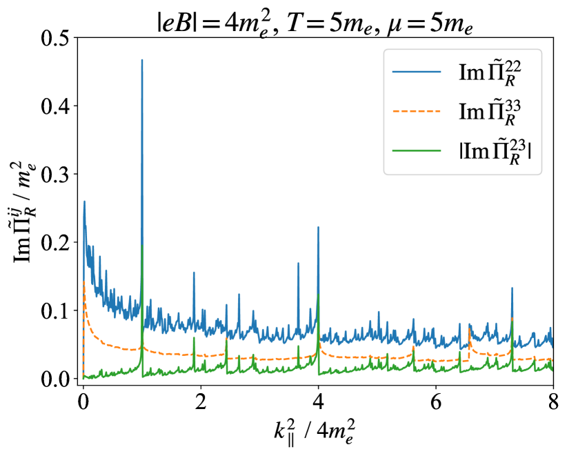
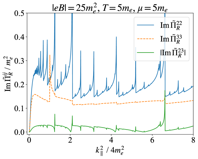
Figure 3: Imaginary part of the polarization tensor components as functions of the photon momentum parallel to the magnetic field for $T=5m_{e},\mu=5m_{e}$, and two fixed magnetic fields: $|eB|=4m_{e}^{2}$ (left panel) and $|eB|=25m_{e}^{2}$ (right panel).

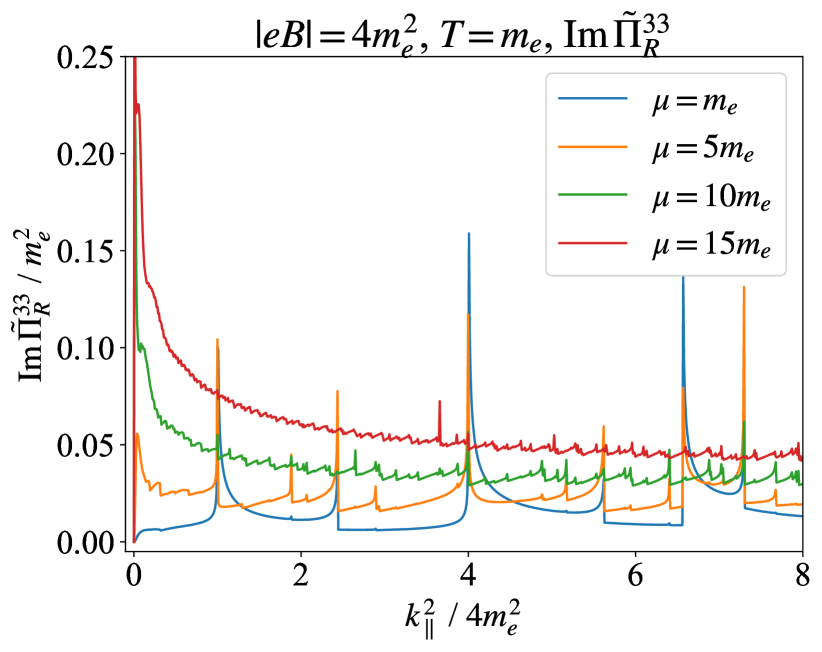
Figure 4: Imaginary part of the $33$-component of the polarization tensor component as a function of the photon momentum parallel to the magnetic field at $|eB|=4m_{e}^{2}$. (Left panel) Dependence on four different values of $T$ at $\mu=0$. (Right panel) Dependence on four different values of $\mu$ at $T=m_{e}$.

4.3 Principal value integral for the real part

To calculate the real part of the polarization tensor $\real\tilde{\Pi}_{R}^{ij}(k)$, we numerically perform the principal value integral (19). In general, we have to deal with the ultraviolet divergence in the vacuum part. However, the ultraviolet divergence vanishes for $k^{2}=0$, so that we can safely conduct the integration; see discussions in ref. Hattori:2012je .

We show the real parts in figure 5. The absolute value of the off-diagonal component is relatively small compared to the diagonal components more manifestly than figure 3 for the imaginary part. The remaining peaky behavior is mainly due to the onsets in the vacuum contribution and the offsets before the onsets arise from the medium effect.

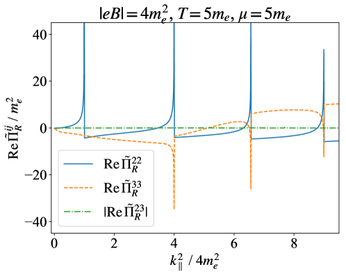
Figure 5: Real part of the polarization tensor as a function of the photon momentum parallel to the magnetic field for $T=5m_{e},\mu=5m_{e},|eB|=4m_{e}^{2}$.

4.4 Photon decay rates

One of the physical quantities given in terms of the photon polarization tensor is the photon decay rates in hot and dense medium:

$$k_{0}\derivative[3]{\Gamma^{\mathrm{X}}}{k}=\dfrac{1}{(2\pi)^{3}}\dfrac{\imaginary\tilde{\Pi}_{R}^{22}}{\mathrm{e}^{\beta k_{0}}-1}\,,\qquad k_{0}\derivative[3]{\Gamma^{\mathrm{O}}}{k}=\dfrac{1}{(2\pi)^{3}}\dfrac{\imaginary\tilde{\Pi}_{R}^{33}}{\mathrm{e}^{\beta k_{0}}-1}\,.$$ (75)

The decay rates for $i=2$ and $3$ correspond to the X-mode photons and the O-mode photons, respectively. The formula contains the processes of the splitting into an electron and a positron in figure 6 and the absorption by an electron and a positron in the magnetized medium in figure 7.

The numerical results of these rates are shown in figure 8. The rate decreases with increasing photon higher energies because of the smaller scattering amplitude of the excitation to the large Landau levels. The peak at $k_{\parallel}^{2}/(4m_{e}^{2})=1$ in figure 8 corresponds to the onset of the splitting process of the photon into a pair of electron and positron.

For practical application, it is important to quantify how much X-mode photons or O-mode photons are more absorbed by the magnetized medium. Thus, we calculate the difference in decay rates of the two modes, and the results are shown in figure 9. The X-mode decay rate ($i=2$) is dominant over the O-mode decay rate ($i=3$) up to the moderate strength of the magnetic field $|eB|\simeq 50m_{e}^{2}$. For the stronger magnetic field case, on the other hand, the O-mode overwhelms the decay rate. For the former observation at weak magnetic field, a semi-classical picture is sensible. Charged particles are accelerated by $B$ which absorb and emit photons with the polarization along the plane of the particle motion orthogonal to the magnetic field. Thus, such photons are X-mode dominated. In contrast, for the strong magnetic field, we can understand the latter from the expected suppression of the X-mode associated with large Landau level gaps. Which is more dominant at extreme environments is crucial for the account of observed polarized photons Lai:2022knd .

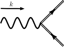
Figure 6: Photon splitting process into an electron and a positron

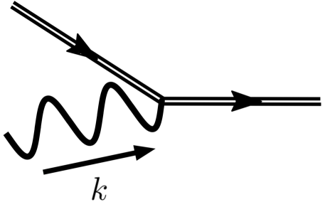
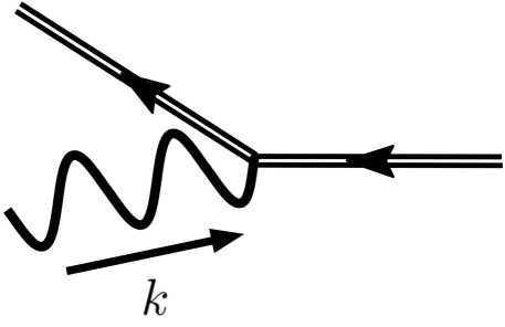
Figure 7: Photon absorption processes by an electron (left panel) and by a positron (right panel).

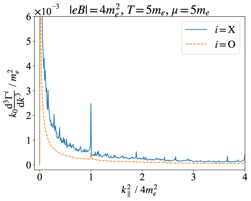
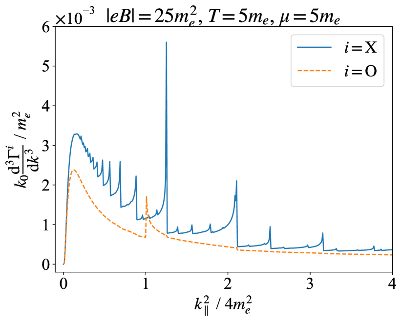
Figure 8: The photon decay rates for two fixed magnetic field: $|eB|=4m_{e}^{2}$ (left panel) and $|eB|=25m_{e}^{2}$ (right panel).

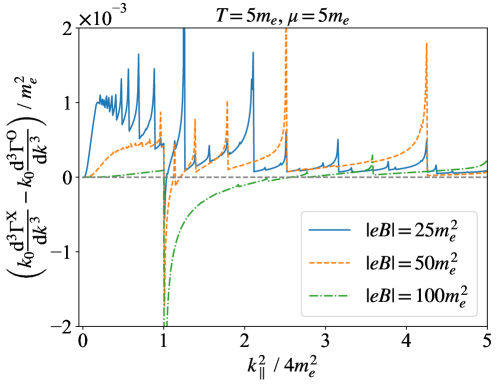
Figure 9: Difference between decay rates of two modes for three fixed magnetic fields: $|eB|=25m_{e}^{2}$, $|eB|=50m_{e}^{2}$, and $|eB|=100m_{e}^{2}$.

5 Conclusions

In this paper, we calculated the photon polarization tensor, $\Pi^{\mu\nu}$, at finite temperature and density in the constant magnetic field. Since the magnetic field breaks rotational symmetry in the system, the structure of the photon polarization tensor becomes complicated. We performed the tensor decomposition and mapped the two transverse components of the polarization tensor to the components parallel and orthogonal to the magnetic field, respectively. For the fermion loop in the polarization tensor, we analytically took the Matsubara sum, imposed the energy conservation constraint, and found closed formulas for the integration with respect to transverse momenta. As a result, we obtained the expressions for $\imaginary\Pi^{\mu\nu}$ which is to be summed numerically over the Landau levels. Specifically, we focused on the real photons with the on-shell condition and summed up the Landau levels for $\imaginary\Pi^{\mu\nu}$ with truncation up to first one hundred levels. We checked the justification of truncation by monitoring that the energy above the truncated level is sufficiently larger than the relevant energy scales of the temperature, the density, and the photon momenta. We then discussed the temperature and the density dependence of $\imaginary\Pi^{\mu\nu}$ which is generally enhanced as the medium effects increase. With resulting $\imaginary\Pi^{\mu\nu}$, we utilized the Kramers-Kronig relation and calculated $\real\Pi^{\mu\nu}$ numerically. Since we focused on the real photons only, no ultraviolet divergence arises in the calculation of the vacuum part of $\real\Pi^{\mu\nu}$ and the renormalization procedure is unnecessary.

The calculation results show how the polarization tensor is sensitive to the polarization modes. For an application example, we evaluated the decay rate of photons with different polarizations in hot and dense magnetized medium. In particular, the decay rate of photons orthogonal to the magnetic field, i.e., X-mode photons, are larger than that of photons parallel to the magnetic field, i.e., O-mode photons as long as the magnetic field is not strong. We also confirmed that the X-mode is suppressed by the Landau level gaps at strong magnetic field and then the O-mode dominates the photon decay rate.

The results in the present work are consistent with the preceding studies and add useful information about the polarization dependence of physical observables. The polarization dependence we have clarified is expected to be applied to phenomenological analyses on electromagnetic probes from hot and dense magnetized QCD matter created in the relativistic heavy-ion collision and polarized photons from the atmosphere at the surface of the magnetar. For a more complete picture for the phenomenological application especially for the polarized photons from the magnetar, we should proceed to higher-order scattering processes and we are making progress along these lines.

Appendix A Formulas for the transverse momentum integration

In this section, we prove the formulas in eqs. (55)-(59).

At first, we compute the following integral:

$$\begin{split}{\mathcal{A}}_{k,l}(z)&=\int\frac{\differential[2]{p_{\perp}}}{(2\pi)^{2}}\mathrm{e}^{-2\xi_{p}}L_{k}(4\xi_{p})\mathrm{e}^{-2\xi_{p-k}}L_{l}(4\xi_{p-k})\,.\end{split}$$ (76)

In order to calculate this, it is useful to remind of the generating functions for the generalized Laguerre polynomials:

$$\sum_{n=0}^{\infty}t^{n}L_{n}^{(\alpha)}(x)=\dfrac{\mathrm{e}^{-tx/(1-t)}}{(1-t)^{\alpha+1}}\,.$$ (77)

Using this, we define the generating function for ${\mathcal{A}}_{k,l}(z)$ as

$$\begin{split}{\mathcal{A}}(s,t,z)\coloneqq&\sum_{k=0}^{\infty}\sum_{l=0}^{\infty}s^{k}t^{l}{\mathcal{A}}_{k,l}(z)\\ =&\frac{1}{1-s}\frac{1}{1-t}\int\frac{\differential[2]{p_{\perp}}}{(2\pi)^{2}}\mathrm{e}^{-2\xi_{p}}\mathrm{e}^{-2\xi_{p-k}}\mathrm{e}^{-\frac{4s}{1-s}\xi_{p}}\mathrm{e}^{-\frac{4t}{1-t}\xi_{p-k}}\\ =&\frac{1}{1-s}\frac{1}{1-t}\int\frac{\differential[2]{p_{\perp}}}{(2\pi)^{2}}\mathrm{e}^{-\frac{1+s}{1-s}\frac{\bm{p}_{\perp}^{2}}{eB}}\mathrm{e}^{-\frac{1+t}{1-t}\frac{\bm{p}_{\perp}^{2}+\bm{k}_{\perp}^{2}-2\bm{p}_{\perp}\cdot\bm{k}_{\perp}}{eB}}\,.\end{split}$$ (78)

Replacing $\alpha=(1+s)/(1-s)$, and $\beta=(1+t)/(1-t)$, we obtain

$$\begin{split}{\mathcal{A}}(s,t,z)&=\frac{1}{1-s}\frac{1}{1-t}\int\frac{\differential[2]{p_{\perp}}}{(2\pi)^{2}}\mathrm{e}^{-\frac{\alpha}{eB}\bm{p}_{\perp}^{2}-\frac{\beta}{eB}(\bm{p}_{\perp}^{2}+\bm{k}_{\perp}^{2}-2\bm{p}_{\perp}\cdot\bm{k}_{\perp})}\\ &=\frac{1}{1-s}\frac{1}{1-t}\int\frac{\differential[2]{p_{\perp}}}{(2\pi)^{2}}\mathrm{e}^{-\frac{\alpha+\beta}{eB}\left(\bm{p}_{\perp}-\frac{\beta}{\alpha+\beta}\bm{k}_{\perp}\right)^{2}-\frac{\alpha\beta}{eB(\alpha+\beta)}\bm{k}_{\perp}^{2}}\,.\end{split}$$ (79)

Conducting Gaussian integration, we find

$$\begin{split}{\mathcal{A}}(s,t,z)&=\frac{1}{1-s}\frac{1}{1-t}\frac{1}{4\pi}\frac{eB}{\alpha+\beta}\mathrm{e}^{-\frac{\alpha\beta}{eB(\alpha+\beta)}\bm{k}_{\perp}^{2}}\\ &=\frac{eB}{8\pi}\mathrm{e}^{-z}\frac{1}{1-st}\mathrm{e}^{-\frac{s+t+2st}{1-st}z}\\ &=\frac{eB}{8\pi}\mathrm{e}^{-z}\sum_{k=0}^{\infty}\sum_{l=0}^{\infty}s^{k}t^{l}\frac{k!}{l!}(-z)^{l-k}\Bigl{[}L_{k}^{(l-k)}(z)\Bigr{]}^{2}\,.\end{split}$$ (80)

Comparing eq. (80) with eq. (78) yields the final result:

$$\begin{split}{\mathcal{A}}_{k,l}(z)&=\frac{eB}{8\pi}\mathrm{e}^{-z}\frac{k!}{l!}(-z)^{l-k}\Bigl{[}L_{k}^{(l-k)}(z)\Bigr{]}^{2}\,.\end{split}$$ (81)

Similarly, the generating functions for other quantities can be introduced as

$$\begin{split}{\mathcal{B}}(s,t,z)&\coloneqq\frac{s}{(1-s)^{2}}\frac{t}{(1-t)^{2}}\int\frac{\differential[2]{p_{\perp}}}{(2\pi)^{2}}\mathrm{e}^{-\frac{\bm{p}_{\perp}^{2}}{eB}}\mathrm{e}^{-\frac{(\bm{p}_{\perp}-\bm{k}_{\perp})^{2}}{eB}}\mathrm{e}^{-\frac{2s}{1-s}\frac{\bm{p}_{\perp}^{2}}{eB}}\mathrm{e}^{-\frac{2t}{1-t}\frac{(\bm{p}_{\perp}-\bm{k}_{\perp})^{2}}{eB}}\times\\ &\qquad\times\left(\bm{p}_{\perp}-\bm{k}_{\perp}\right)\cdot\bm{p}_{\perp}\\ &=\frac{(eB)^{2}}{16\pi}\frac{st}{(1-st)^{2}}\left[1-\frac{(1+s)(1+t)}{1-st}z\right]\mathrm{e}^{-\frac{(1+s)(1+t)}{1-st}z}\\ &=\frac{(eB)^{2}}{16\pi}\frac{st}{(1-st)^{2}}\left(1+z\frac{d}{dz}\right)\mathrm{e}^{-\frac{(1+s)(1+t)}{1-st}z}\\ &=\frac{(eB)^{2}}{16\pi}\mathrm{e}^{-z}\sum_{k=1}^{\infty}\sum_{l=1}^{\infty}s^{k}t^{l}\frac{k!}{(l-1)!}(-z)^{l-k}L_{k}^{(l-k)}(z)L_{k-1}^{(l-k)}(z)\,,\end{split}$$ (82)

$$\begin{split}{\mathcal{C}}(s,t,z)&\coloneqq\frac{s}{(1-s)^{2}}\frac{t}{(1-t)^{2}}\int\frac{\differential[2]{p_{\perp}}}{(2\pi)^{2}}\mathrm{e}^{-\frac{\bm{p}_{\perp}^{2}}{eB}}\mathrm{e}^{-\frac{(\bm{p}_{\perp}-\bm{k}_{\perp})^{2}}{eB}}\mathrm{e}^{-\frac{2s}{1-s}\frac{\bm{p}_{\perp}^{2}}{eB}}\mathrm{e}^{-\frac{2t}{1-t}\frac{(\bm{p}_{\perp}-\bm{k}_{\perp})^{2}}{eB}}\times\\ &\qquad\times\left[\bm{p}_{\perp}\cdot\bm{k}_{\perp}-\frac{2(\bm{p}_{\perp}\cdot\bm{k}_{\perp})^{2}}{\bm{k}_{\perp}^{2}}+\bm{p}_{\perp}^{2}\right]\\ &=\frac{(eB)^{2}}{16\pi}\frac{st(1+s)(1+t)}{(1-st)^{3}}z\mathrm{e}^{-\frac{(1+s)(1+t)}{1-st}z}\\ &=\frac{(eB)^{2}}{16\pi}\mathrm{e}^{-z}\sum_{k=1}^{\infty}\sum_{l=1}^{\infty}s^{k}t^{l}\frac{k!}{(l-1)!}(-z)^{l-k}\times\\ &\qquad\times\left[\frac{k}{z}F(k,l,z)-\frac{k+l}{z}L_{k}^{(l-k)}(z)L_{k-1}^{(l-k)}(z)\right]\,,\end{split}$$ (83)

$$\begin{split}{\mathcal{D}}(s,t,z)&\coloneqq\frac{s}{(1-s)^{2}}\frac{t}{(1-t)^{2}}\int\frac{\differential[2]{p_{\perp}}}{(2\pi)^{2}}\mathrm{e}^{-\frac{\bm{p}_{\perp}^{2}}{eB}}\mathrm{e}^{-\frac{(\bm{p}_{\perp}-\bm{k}_{\perp})^{2}}{eB}}\mathrm{e}^{-\frac{2s}{1-s}\frac{\bm{p}_{\perp}^{2}}{eB}}\mathrm{e}^{-\frac{2t}{1-t}\frac{(\bm{p}_{\perp}-\bm{k}_{\perp})^{2}}{eB}}\times\\ &\qquad\times\left[2\bm{p}_{\perp}^{2}-\frac{2(\bm{p}_{\perp}\cdot\bm{k}_{\perp})^{2}}{\bm{k}_{\perp}^{2}}\right]\\ &=\frac{(eB)^{2}}{16\pi}\frac{st}{(1-st)^{2}}\mathrm{e}^{-\frac{(1+s)(1+t)}{1-st}z}\\ &=\frac{(eB)^{2}}{16\pi}\mathrm{e}^{-z}\sum_{k=1}^{\infty}\sum_{l=1}^{\infty}s^{k}t^{l}\frac{k!}{(l-1)!}(-z)^{l-k}\times\\ &\qquad\times\biggl{[}\frac{k}{z}F(k,l,z)-\frac{k+l-z}{z}L_{k}^{(l-k)}(z)L_{k-1}^{(l-k)}(z)\biggr{]}\,,\end{split}$$ (84)

and

$$\begin{split}\mathcal{E}(s,t,z)&\coloneqq\frac{s}{(1-s)^{2}}\frac{1}{1-t}\int\frac{\differential[2]{p_{\perp}}}{(2\pi)^{2}}\mathrm{e}^{-\frac{\bm{p}_{\perp}^{2}}{eB}}\mathrm{e}^{-\frac{(\bm{p}_{\perp}-\bm{k}_{\perp})^{2}}{eB}}\mathrm{e}^{-\frac{2s}{1-s}\frac{\bm{p}_{\perp}^{2}}{eB}}\mathrm{e}^{-\frac{2t}{1-t}\frac{(\bm{p}_{\perp}-\bm{k}_{\perp})^{2}}{eB}}\left(\bm{p}_{\perp}\cdot\bm{k}_{\perp}\right)\\ &=\frac{(eB)^{2}}{16\pi}\frac{2s(1+t)}{(1-st)^{2}}z\mathrm{e}^{-\frac{(1+s)(1+t)}{1-st}z}\\ &=2z\biggl{[}\frac{1}{t}{\mathcal{D}}(s,t,z)+{\mathcal{D}}(s,t,z)\biggr{]}\\ &=\sum_{k=1}^{\infty}\sum_{l=0}^{\infty}s^{k}t^{l}2z\bigl{[}D_{k,l+1}(z)+D_{k,l}(z)\bigr{]}\,.\end{split}$$ (85)

With these generating functions, the formulas of our interest are immediately recovered.

References

- (1) E.S. Fraga and A.J. Mizher, Chiral transition in a strong magnetic background, Phys. Rev. D 78 (2008) 025016 [0804.1452].
- (2) A.J. Mizher, M.N. Chernodub and E.S. Fraga, Phase diagram of hot QCD in an external magnetic field: possible splitting of deconfinement and chiral transitions, Phys. Rev. D 82 (2010) 105016 [1004.2712].
- (3) E.J. Ferrer, V. de la Incera, I. Portillo and M. Quiroz, New look at the QCD ground state in a magnetic field, Phys. Rev. D 89 (2014) 085034 [1311.3400].
- (4) R. Gatto and M. Ruggieri, Dressed Polyakov loop and phase diagram of hot quark matter under magnetic field, Phys. Rev. D 82 (2010) 054027 [1007.0790].
- (5) R. Gatto and M. Ruggieri, Deconfinement and Chiral Symmetry Restoration in a Strong Magnetic Background, Phys. Rev. D 83 (2011) 034016 [1012.1291].
- (6) M. Ferreira, P. Costa, O. Lourenço, T. Frederico and C. Providência, Inverse magnetic catalysis in the (2+1)-flavor Nambu-Jona-Lasinio and Polyakov-Nambu-Jona-Lasinio models, Phys. Rev. D 89 (2014) 116011 [1404.5577].
- (7) N. Mueller and J.M. Pawlowski, Magnetic catalysis and inverse magnetic catalysis in QCD, Phys. Rev. D 91 (2015) 116010 [1502.08011].
- (8) K.G. Klimenko, Three-dimensional Gross-Neveu model at nonzero temperature and in an external magnetic field, Z. Phys. C 54 (1992) 323.
- (9) V.P. Gusynin, V.A. Miransky and I.A. Shovkovy, Catalysis of dynamical flavor symmetry breaking by a magnetic field in (2+1)-dimensions, Phys. Rev. Lett. 73 (1994) 3499 [hep-ph/9405262].
- (10) V.P. Gusynin, V.A. Miransky and I.A. Shovkovy, Dimensional reduction and catalysis of dynamical symmetry breaking by a magnetic field, Nucl. Phys. B 462 (1996) 249 [hep-ph/9509320].
- (11) I.A. Shushpanov and A.V. Smilga, Quark condensate in a magnetic field, Phys. Lett. B 402 (1997) 351 [hep-ph/9703201].
- (12) K. Fukushima and J.M. Pawlowski, Magnetic catalysis in hot and dense quark matter and quantum fluctuations, Phys. Rev. D 86 (2012) 076013 [1203.4330].
- (13) G.S. Bali, F. Bruckmann, G. Endrödi and A. Schäfer, Magnetization and pressures at nonzero magnetic fields in QCD, PoS LATTICE2013 (2014) 182 [1310.8145].
- (14) V.A. Miransky and I.A. Shovkovy, Quantum field theory in a magnetic field: From quantum chromodynamics to graphene and Dirac semimetals, Phys. Rept. 576 (2015) 1 [1503.00732].
- (15) M. D’Elia, S. Mukherjee and F. Sanfilippo, QCD Phase Transition in a Strong Magnetic Background, Phys. Rev. D 82 (2010) 051501 [1005.5365].
- (16) G.S. Bali, F. Bruckmann, G. Endrodi, Z. Fodor, S.D. Katz, S. Krieg et al., The QCD phase diagram for external magnetic fields, JHEP 02 (2012) 044 [1111.4956].
- (17) G. Endrodi, QCD with background electromagnetic fields on the lattice: a review, 2406.19780.
- (18) G.S. Bali, F. Bruckmann, G. Endrodi, Z. Fodor, S.D. Katz and A. Schafer, QCD quark condensate in external magnetic fields, Phys. Rev. D 86 (2012) 071502 [1206.4205].
- (19) F. Bruckmann, G. Endrodi and T.G. Kovacs, Inverse magnetic catalysis and the Polyakov loop, JHEP 04 (2013) 112 [1303.3972].
- (20) Y. Hidaka and A. Yamamoto, Charged vector mesons in a strong magnetic field, Phys. Rev. D 87 (2013) 094502 [1209.0007].
- (21) K. Hattori, T. Kojo and N. Su, Mesons in strong magnetic fields: (I) General analyses, Nucl. Phys. A 951 (2016) 1 [1512.07361].
- (22) H.-T. Ding, S.-T. Li, S. Mukherjee, A. Tomiya and X.-D. Wang, Meson masses in external magnetic fields with HISQ fermions, PoS LATTICE2019 (2020) 250 [2001.05322].
- (23) V. Skokov, A.Y. Illarionov and V. Toneev, Estimate of the magnetic field strength in heavy-ion collisions, Int. J. Mod. Phys. A 24 (2009) 5925 [0907.1396].
- (24) V. Voronyuk, V.D. Toneev, W. Cassing, E.L. Bratkovskaya, V.P. Konchakovski and S.A. Voloshin, (Electro-)Magnetic field evolution in relativistic heavy-ion collisions, Phys. Rev. C 83 (2011) 054911 [1103.4239].
- (25) W.-T. Deng and X.-G. Huang, Event-by-event generation of electromagnetic fields in heavy-ion collisions, Phys. Rev. C 85 (2012) 044907 [1201.5108].
- (26) L. McLerran and V. Skokov, Comments About the Electromagnetic Field in Heavy-Ion Collisions, Nucl. Phys. A 929 (2014) 184 [1305.0774].
- (27) D.E. Kharzeev, L.D. McLerran and H.J. Warringa, The Effects of topological charge change in heavy ion collisions: ’Event by event P and CP violation’, Nucl. Phys. A 803 (2008) 227 [0711.0950].
- (28) K. Fukushima, D.E. Kharzeev and H.J. Warringa, The Chiral Magnetic Effect, Phys. Rev. D 78 (2008) 074033 [0808.3382].
- (29) D.T. Son and A.R. Zhitnitsky, Quantum anomalies in dense matter, Phys. Rev. D 70 (2004) 074018 [hep-ph/0405216].
- (30) M.A. Metlitski and A.R. Zhitnitsky, Anomalous axion interactions and topological currents in dense matter, Phys. Rev. D 72 (2005) 045011 [hep-ph/0505072].
- (31) D.T. Son and P. Surowka, Hydrodynamics with Triangle Anomalies, Phys. Rev. Lett. 103 (2009) 191601 [0906.5044].
- (32) D.E. Kharzeev and D.T. Son, Testing the chiral magnetic and chiral vortical effects in heavy ion collisions, Phys. Rev. Lett. 106 (2011) 062301 [1010.0038].
- (33) D. Kharzeev, Parity violation in hot QCD: Why it can happen, and how to look for it, Phys. Lett. B 633 (2006) 260 [hep-ph/0406125].
- (34) D.E. Kharzeev, The Chiral Magnetic Effect and Anomaly-Induced Transport, Prog. Part. Nucl. Phys. 75 (2014) 133 [1312.3348].
- (35) S. Shi, Y. Jiang, E. Lilleskov and J. Liao, Anomalous Chiral Transport in Heavy Ion Collisions from Anomalous-Viscous Fluid Dynamics, Annals Phys. 394 (2018) 50 [1711.02496].
- (36) D.E. Kharzeev, J. Liao, S.A. Voloshin and G. Wang, Chiral magnetic and vortical effects in high-energy nuclear collisions—A status report, Prog. Part. Nucl. Phys. 88 (2016) 1 [1511.04050].
- (37) STAR collaboration, Global hyperon polarization in nuclear collisions: evidence for the most vortical fluid, Nature 548 (2017) 62 [1701.06657].
- (38) Z.-T. Liang and X.-N. Wang, Globally polarized quark-gluon plasma in non-central A+A collisions, Phys. Rev. Lett. 94 (2005) 102301 [nucl-th/0410079].
- (39) F. Becattini, I. Karpenko, M. Lisa, I. Upsal and S. Voloshin, Global hyperon polarization at local thermodynamic equilibrium with vorticity, magnetic field and feed-down, Phys. Rev. C 95 (2017) 054902 [1610.02506].
- (40) M.G. Alford, J. Berges and K. Rajagopal, Magnetic fields within color superconducting neutron star cores, Nucl. Phys. B 571 (2000) 269 [hep-ph/9910254].
- (41) E.J. Ferrer, V. de la Incera and C. Manuel, Magnetic color flavor locking phase in high density QCD, Phys. Rev. Lett. 95 (2005) 152002 [hep-ph/0503162].
- (42) E.J. Ferrer, V. de la Incera and C. Manuel, Color-superconducting gap in the presence of a magnetic field, Nucl. Phys. B 747 (2006) 88 [hep-ph/0603233].
- (43) J.L. Noronha and I.A. Shovkovy, Color-flavor locked superconductor in a magnetic field, Phys. Rev. D 76 (2007) 105030 [0708.0307].
- (44) K. Fukushima and H.J. Warringa, Color superconducting matter in a magnetic field, Phys. Rev. Lett. 100 (2008) 032007 [0707.3785].
- (45) T. Brauner and N. Yamamoto, Chiral Soliton Lattice and Charged Pion Condensation in Strong Magnetic Fields, JHEP 04 (2017) 132 [1609.05213].
- (46) S. Chen, K. Fukushima and Z. Qiu, Skyrmions in a magnetic field and 0 domain wall formation in dense nuclear matter, Phys. Rev. D 105 (2022) L011502 [2104.11482].
- (47) Z. Qiu and M. Nitta, Quasicrystals in QCD, JHEP 05 (2023) 170 [2304.05089].
- (48) G.W. Evans and A. Schmitt, Chiral Soliton Lattice turns into 3D crystal, JHEP 2024 (2024) 041 [2311.03880].
- (49) R. Taverna, R. Turolla, V. Suleimanov, A.Y. Potekhin and S. Zane, X-ray spectra and polarization from magnetar candidates, Mon. Not. Roy. Astron. Soc. 492 (2020) 5057 [2001.07663].
- (50) R. Taverna et al., Polarized x-rays from a magnetar, 2205.08898.
- (51) R. Taverna and R. Turolla, X-ray Polarization from Magnetar Sources, Galaxies 12 (2024) 6 [2402.05622].
- (52) S. Zane et al., A Strong X-Ray Polarization Signal from the Magnetar 1RXS J170849.0-400910, Astrophys. J. Lett. 944 (2023) L27 [2301.12919].
- (53) R. Turolla et al., IXPE and XMM-Newton Observations of the Soft Gamma Repeater SGR 1806–20, Astrophys. J. 954 (2023) 88 [2308.01238].
- (54) D. Lai and W.C.G. Ho, Polarized x-ray emission from magnetized neutron stars: Signature of strong - field vacuum polarization, Phys. Rev. Lett. 91 (2003) 071101 [astro-ph/0303596].
- (55) D. Lai, IXPE detection of polarized X-rays from magnetars and photon mode conversion at QED vacuum resonance, Proc. Nat. Acad. Sci. 120 (2023) e2216534120 [2209.13640].
- (56) W. Heisenberg and H. Euler, Consequences of Dirac’s theory of positrons, Z. Phys. 98 (1936) 714 [physics/0605038].
- (57) J.S. Schwinger, On gauge invariance and vacuum polarization, Phys. Rev. 82 (1951) 664.
- (58) G.V. Dunne, Heisenberg-Euler effective Lagrangians: Basics and extensions, in From fields to strings: Circumnavigating theoretical physics. Ian Kogan memorial collection (3 volume set), M. Shifman, A. Vainshtein and J. Wheater, eds., pp. 445–522 (2004), DOI [hep-th/0406216].
- (59) E.J. Ferrer, V. de la Incera and A. Sanchez, Non-perturbative Euler-Heisenberg Lagrangian and Paraelectricity in Magnetized Massless QED, Nucl. Phys. B 864 (2012) 469 [1204.3660].
- (60) V.N. Baier and V.M. Katkov, Pair creation by a photon in a strong magnetic field, Phys. Rev. D 75 (2007) 073009 [hep-ph/0701119].
- (61) K. Hattori and K. Itakura, Vacuum birefringence in strong magnetic fields: (I) Photon polarization tensor with all the Landau levels, Annals Phys. 330 (2013) 23 [1209.2663].
- (62) K. Hattori and K. Itakura, Vacuum birefringence in strong magnetic fields: (II) Complex refractive index from the lowest Landau level, Annals Phys. 334 (2013) 58 [1212.1897].
- (63) J. Alexandre, Vacuum polarization in thermal QED with an external magnetic field, Phys. Rev. D 63 (2001) 073010 [hep-th/0009204].
- (64) X. Wang, I.A. Shovkovy, L. Yu and M. Huang, Ellipticity of photon emission from strongly magnetized hot QCD plasma, Phys. Rev. D 102 (2020) 076010 [2006.16254].
- (65) X. Wang and I. Shovkovy, Photon polarization tensor in a magnetized plasma: Absorptive part, Phys. Rev. D 104 (2021) 056017 [2103.01967].
- (66) X. Wang and I. Shovkovy, Polarization tensor of magnetized quark-gluon plasma at nonzero baryon density, Eur. Phys. J. C 81 (2021) 901 [2106.09029].
- (67) K. Hattori and K. Itakura, In-medium polarization tensor in strong magnetic fields (I): Magneto-birefringence at finite temperature and density, Annals Phys. 446 (2022) 169114 [2205.04312].
- (68) K. Hattori and K. Itakura, In-medium polarization tensor in strong magnetic fields (II): Axial Ward identity at finite temperature and density, Annals Phys. 446 (2022) 169115 [2205.06411].
- (69) P.K. Pyatkovskiy and V.P. Gusynin, Dynamical polarization of monolayer graphene in a magnetic field, Phys. Rev. B 83 (2011) 075422 [1009.5980].
- (70) H. Perez Rojas and A.E. Shabad, POLARIZATION OF RELATIVISTIC ELECTRON AND POSITRON GAS IN A STRONG MAGNETIC FIELD. PROPAGATION OF ELECTROMAGNETIC WAVES, Annals Phys. 121 (1979) 432.