Effect of Coriolis Force on Diffusion of D Meson

Abstract

We have attempted to calculate and estimate the diffusion coefficients of D meson through rotating hadron resonance gas, which can be produced in the late stage of peripheral heavy ion collisions. According to the kinetic theory framework of relaxation time approximation and Einstein’s diffusion relation, one can express D meson diffusion as a ratio of its conductivity to its susceptibility. Here, we have tuned D meson relaxation time from the knowledge of earlier works on its spatial diffusion estimations, and then we have extended the framework for the finite rotation picture of hadronic matter, where only the effect of Coriolis force is considered. The ratio of shear viscosity to entropy density shows a valley-shaped pattern well-known in the community of heavy-ion physics. Diffusion coefficients of D meson show a similar structure. Our study also revealed the anisotropic nature of diffusion in the presence of rotation with future possibilities of phenomenological signature.

I Introduction

Quark-Gluon Plasma (QGP), a QCD state of matter, is expected to form in ultra-relativistic heavy-ion collisions (HICs) [1, 2]. Hard partons and heavy quarks (HQs) are profusely produced at Relativistic Heavy Ion Collider (RHIC) and Large Hadron Collider (LHC) energies in initial hard scattering processes. They are sensitive probes of the medium formed in the collision as they are produced at the early stages of the collision and witness the entire evolution of the QGP [3, 4, 5, 6, 7, 8, 9, 10, 11]. HQs may lose energy by collisions as well as by gluon bremsstrahlung while propagating through the medium [12, 13, 14, 15, 16, 17, 18]. The energy loss of the HQs inside the medium can be quantified by measuring the transverse momentum suppression ($R_{AA}$) [19], which may be considered as an indirect measurement of the drag and diffusion coefficient of charm quark in QGP [20, 21, 22]. For a comprehensive review of different transport models of HQ and hadronization mechanisms, one can see the Refs. [23, 24]. HQ transport in the pre-equilibrium phase of the QGP has also been studied in Refs. [25, 28, 26, 27, 29]. An extremely strong magnetic field (of the order of $10^{18}$ to $10^{19}$ Gauss [30]) is expected to produce in peripheral heavy-ion collision [31, 32]. A strong magnetic field may influence the relativistic fluids, and thus flow [33], jet quenching coefficient [34], heavy quark/ meson diffusion coefficients [35], etc. may be affected. The diffusion phenomenology of the heavy quarks and meson at a finite magnetic field was discussed in Ref. [35]. In off-central HICs, along with the creation of huge magnetic fields, a large orbital angular momentum (OAM) can also be transferred from the initial colliding nuclei to the formed medium [36, 37]. In this respect, the medium formed in off-central collisions at the RHIC can be considered to be a rotating system, possessing a significant OAM ranging up to $10^{7}\hbar$ [38, 36, 37]. This initial OAM subsequently manifests itself as local vorticity first in the quark fluid and later in the hadronic fluid. The vorticity can result in various effects such as spin polarization [39], the chiral vortical effect (CVE) [40], etc. The STAR Collaboration measured the global spin polarization of $\Lambda$ and $\bar{\Lambda}$ particles in Au + Au collisions over a range of collision energies ($\sqrt{s_{NN}}=$ 7.7-200 GeV), revealing a decreasing trend with collision energies [38]. A recent study with better statistics at $\sqrt{s_{NN}}=$ 200 GeV found that polarization depends on event-by-event charge asymmetry. This suggests that the axial current induced by the initial magnetic field might contribute to global polarization [41]. Furthermore, spin alignment has been observed in vector mesons, with recent measurements at the RHIC and LHC enhancing our understanding of spin phenomena in heavy ion collisions [42, 43, 44]. Moreover, the presence of Coriolis force in a rotating medium can also lead to anisotropic diffusion coefficients of HQs and mesons as previously studied in the presence of Lorentz force because of magnetic fields [35]. In the present work, we will focus on the diffusion phenomenology of heavy mesons due to the presence of Coriolis force in the rotating medium.

There is a notable connection between rotational effects and magnetic fields, both of which can be produced in off-central collisions. The Coriolis force, arising from rotation, and the Lorentz force, generated in the presence of magnetic fields, exhibit striking similarities in their effects on moving particles Refs. [45, 46, 47]. The presence of magnetic fields induces anisotropy in the transport coefficients and this anisotropy in the context of viscosities and conductivities of the produced nuclear matter in HICs has been investigated in Refs. [48, 49, 50, 51, 52, 53, 54, 55, 56, 57, 48, 58, 59, 60, 61]. Apart from these studies of transport coefficients of QGP and hadronic gases in the presence of magnetic fields, the effect of magnetic fields in the dynamics of HQs inside the QGP and the hadronic system has also been studied. Initial studies on the dynamics of $J/\psi$ mesons have used holographic QCD to explore the influence of magnetic fields on charmonium [62]. Simplified holographic QCD models have also been employed to examine the transport properties of $J/\psi$ and heavy quarks, showing that spatial diffusion is split into longitudinal and transverse components based on the direction of the magnetic field [63, 35]. Due to the similarity in the expression of Coriolis force and Lorentz force, one can expect a similar nature of transport phenomena in a rotating medium and a medium in the presence of magnetic fields. In connection to this the Ref. [64, 65, 66] have explored the similarity between the Coriolis force and Lorentz force to calculate the anisotropic transport coefficients of QGP and hadronic matter. Specifically, the anisotropic nature of shear viscosity and electrical conductivity in the presence of the Coriolis force was observed in Refs. [64, 65] in a non-relativistic framework. The effect of Coriolis force in the electrical conductivity of a hadron gas was also studied in a relativistic framework by employing the Hadron Resonance Gas (HRG) model in Ref. [66]. Aside from the transport phenomena of rotating QGP and hadronic medium, the HQs and mesons transport can be significantly affected inside a rotating QGP or hadronic medium. In particular, the diffusion coefficients of heavy mesons can also exhibit a similar structure in a rotating medium as it exhibits in the presence of magnetic fields [63, 35]. Nevertheless, the dynamics of heavy mesons inside a rotating medium have not been addressed thoroughly in the literature. If we see earlier references for diffusion calculation in the absence of magnetic fields or medium rotation, then we will get a long list of Refs. [20, 21, 22, 67], which is focused on the heavy quark diffusion in QGP. However, heavy meson or baryon diffusion in hadronic matter topics was completely ignored or overlooked before 2010 by assuming its negligible contribution. It was Refs.[68, 69] who addressed the non-negligible contribution of heavy meson or baryon diffusion in the hadronic matter. For a recent review of the transport of the open heavy flavors inside hadronic matter, one can see Ref. [70]. In this paper, we extend the exploration of rotating effects to the diffusion of heavy mesons ($D$ meson) inside the hadron gas. To fulfill this goal, we first write the relativistic Boltzmann transport equation (BTE) for $D$ meson distribution in a rotating frame of reference by adhering to the relaxation time approximation (RTA). The generalization of BTE to the rotating frame of references has been made with the aid of connection coefficients, which in turn can be calculated from the space-dependent rotating frame metric. The relaxation time of the $D$ meson with the background hadronic gas has been calculated by the popular HRG model. The HRG is a well-established model for describing the hadronic phase of matter produced in relativistic heavy ion collisions. In this framework, the system can be effectively treated as a multi-species gas consisting of various particles such as protons, neutrons, and pions along with the numerous unstable resonant states documented by the Particle Data Group [71]. The HRG model has been widely used to explore a wide range of phenomena, including HIC thermodynamics [72, 73, 74, 75] and fluctuations of conserved charges [76, 77, 78, 79, 80, 81]. The HRG model has proven valuable in estimating various transport coefficients that govern the system’s response to external forces  [82, 83, 84, 85, 86, 87, 88, 89, 90, 91, 92, 93]. In this investigation, we use an ideal HRG model for the estimation of $D$ meson diffusion in rotating HRG medium.

The article is arranged as follows. At the beginning of Sec. II, we recapitulate the previous works that dealt with transport coefficients of rotating nuclear matter and give a general layout for calculating the diffusion of $D$ meson through the rotating hadronic matter. Afterward, in Sec. II.1, we first develop the covariant BTE in the rotating frame by illustrating the different kinds of forces that affect the meson transport. Secondly, we calculate the diffusion tensor of the meson with the help of BTE in RTA. Then, in Sec. II.2, we briefly describe the HRG model, which we use to determine the $D$ meson relaxation time by assuming hard sphere scattering interactions. In Sec. III, we display the numerical estimations of the conductivity and diffusion of the $D$ meson and quantitatively discuss the anisotropy produced because of the rotation. Ultimately, we summarize our findings in Sec. IV. In the end, an appendix discusses the detailed derivation of heavy meson conductivity from the relativistic Boltzmann equation.

II Methodology and Model descriptions

In the previous works related to transport in the rotating nuclear medium, the Refs. [64, 65] have explored the structure of shear viscosity and electrical conductivity of a rotating QGP using Non-relativistic BTE. This calculation for the rotating nuclear matter has been extended recently to the relativistic realm in Ref. [66], where the covariant BTE is used to obtain the anisotropic conductivities for hadronic gas employing the popular HRG model. All these models have a common physical picture in which one explicitly incorporates the rotational background of the medium expected in off-central HIC in the kinetic description. Subsequently, one writes down a BTE in the rotating frame to calculate the transport properties of the QGP and the hadronic gas. Here, in contrast to the aim of the Refs. [64, 65, 66], we will be concerned with the diffusion of open charmed mesons ($D$ meson) through the rotating hadronic matter. In order to address this diffusion phenomenon, the mathematical framework of Ref. [66] can be borrowed with following important changes: the equation of motion (EOM) in the rotating frame will be that of the $D$ meson which diffuse in the background light hadrons and the covariant BTE will be set up for the distribution function of $D$ meson to determine the diffusion coefficients.

Now, let us begin by defining the dissipative current density and conductivity tensor of the $D$ meson, which we will directly connect with the diffusion coefficients later in Sec. II.1. The microscopic and macroscopic expression for the dissipative current density $J^{i}$ of the $D$ meson diffusing under a rotating hadronic background can be written as,

$$J^{i} = \int\frac{d^{3}\vec{p}}{(2\pi)^{3}}\frac{p^{i}}{p_{0}}~{}\delta f,$$ (1)

$$J^{i} = -\sigma^{ij}\nabla_{j}\mu_{D},$$ (2)

where $\mu_{D}$, $p_{0}=E$, $\delta f$ are respectively the charm meson chemical potential, energy and out-of-equilibrium part of the distribution function associated with the $D$ meson. The Eq. (1) provides the kinetic definition of the $D$ meson current, which can be evaluated by determining the out-of-equilibrium distribution $\delta f$ by solving the BTE in a rotating frame. On the other hand, Eq. (2) is reminiscent of Ohm’s law with the driving force as the electric field had replaced by the negative gradient of $\mu_{D}$. After evaluating $J^{i}$ from Eq. (1) with the help of BTE, one can obtain the $D$ meson conductivity tensor $\sigma^{ij}$ by comparing Eq. (1) with Eq. (2). Then, the diffusion coefficients of $D$ meson can be obtained by taking the ratio of its conductivity tensor with susceptibility.

Having discussed this general layout of obtaining the diffusion coefficients, we will now proceed to the next subsection for the explicit calculation of $D$ meson conductivities and diffusion coefficients from the BTE.

II.1 Diffusion coefficients for $\mathbf{D}$ meson

In this section, our final goal will be to write down the covariant BTE in the rotating frame and evaluate the diffusion coefficients for the $D$ meson. Before moving towards our final goal, we will briefly describe the mathematical tools needed in the procedure; interested readers can get the detailed mathematical framework in Ref. [66]. The coordinate transformation from inertial coordinates ${\bf x}\equiv(t,x,y,z)$ to rotating coordinates ${\bf x}^{\prime}\equiv(t^{\prime},x^{\prime},y^{\prime},z^{\prime})$ [94, 95, 96, 97]:

$${\bf x}^{\prime}=\mathbf{R}(\Omega t)~{}{\bf x},$$ (3)

is essential to describe the EOM of $D$ meson in a rotating frame, where the rotation matrix $\mathbf{R}(\Omega t)$ for transforming coordinates from the inertial frame to the rotating frame is given by:

$$\mathbf{R}(\Omega t)=\begin{pmatrix}1&0&0&0\\ 0&\cos(\Omega t)&\sin(\Omega t)&0\\ 0&-\sin(\Omega t)&\cos(\Omega t)&0\\ 0&0&0&1\end{pmatrix}.$$ (4)

Using the transformation law provided in Eq. (3) and (4) one can obtain the squared length element $ds^{2}$, metric tensor $g_{\mu\nu}$ and connection coefficients $\Gamma_{\mu\lambda}^{\alpha}$ as follows[66]:

$$ds^{2}=g_{\mu\nu}dx^{\prime\mu}dx^{\prime\nu}=dt^{\prime^{2}}(1-\Omega^{2}x^{\prime^{2}}-\Omega^{2}y^{\prime^{2}})+2\Omega y^{\prime}dt^{\prime}dx^{\prime}-2\Omega x^{\prime}dt^{\prime}dy^{\prime}-dx^{\prime^{2}}-dy^{\prime^{2}}-dz^{\prime^{2}},$$

$$g_{\mu\nu}=\begin{pmatrix}1-\Omega^{2}x^{\prime^{2}}-\Omega^{2}y^{\prime^{2}}&\Omega y^{\prime}&-\Omega x^{\prime}&0\\ \Omega y^{\prime}&-1&0&0\\ -\Omega x^{\prime}&0&-1&0\\ 0&0&0&-1\end{pmatrix},$$ (5)

$$\Gamma_{\mu\lambda}^{\alpha}=\frac{1}{2}g^{\alpha\nu}\left(\frac{\partial g_{\nu\mu}}{\partial x^{\lambda}}+\frac{\partial g_{\lambda\nu}}{\partial x^{\mu}}-\frac{\partial g_{\mu\lambda}}{\partial x^{\nu}}\right).$$ (6)

Now, we are ready to write down the EOM for the $D$ meson, which will eventually be required to establish the BTE for the $D$ meson diffusion. The EOM for the $D$ meson in the rotating frame is given by [98, 99, 100]:

$$\frac{dp^{\alpha}}{d\tau}+\frac{1}{m_{D}}p^{\mu}p^{\lambda}\Gamma_{\mu\lambda}^{\alpha}=0,$$ (7)

where $p^{\alpha}$ and $\tau$ are the four-momentum and proper time, respectively. The non zero connection coefficients in the present case can be obtained by resorting to Eq. (5) and (6) as follows [101]: $\Gamma_{00}^{1}=-\Omega^{2}x,\Gamma_{00}^{2}=-\Omega^{2}y,\Gamma_{20}^{1}=\Gamma_{02}^{1}=-\Omega,\Gamma_{10}^{2}=\Gamma_{01}^{2}=\Omega$. Let us recast Eq. (7) with the substitution of non-zero connection coefficients in order to observe the resemblance between the EOM of $D$ meson supplied by Eq. (7) and the classical nonrelativistic EOM in the rotating frame [102, 103],

$$\frac{d\vec{p}}{dt}=\gamma_{v}m_{D}(\vec{\Omega}\times\vec{r})\times\vec{\Omega}+2\gamma_{v}m_{D}(\vec{v}\times\vec{\Omega}),$$ (8)

where the four-momentum is given by, $p^{\alpha}=(\gamma_{v}m_{D},\gamma_{v}m_{D}\vec{v})=(\gamma_{v}m_{D},\vec{p})$ with the Loretz factor $\gamma_{v}=\frac{dt}{d\tau}$. A quick glance at Eq. (8) suggests that the first and second terms in the RHS of Eq. (8) are the relativistic version of the centrifugal force and Coriolis force, respectively. Now, we are equipped with all the necessary tools to write down the BTE for $D$ meson diffusing under the rotating hadronic background. The covariant BTE in the co-rotating frame can be written as:

$$p^{\mu}\frac{\partial f}{\partial x^{\mu}}-m_{D}\frac{dp^{\alpha}}{d\tau}\frac{\partial f}{\partial p^{\alpha}}=C[f]$$

$$\implies p^{\mu}\frac{\partial f}{\partial x^{\mu}}-\Gamma_{\mu\lambda}^{\alpha}p^{\mu}p^{\lambda}\frac{\partial f}{\partial p^{\alpha}}=-(u^{\alpha}p_{\alpha})\frac{\delta f}{\tau_{c}},$$ (9)

where we used Eq. (7) and approximated the collision kernel $C[f]$ by the RTA i.e., $C[f]\thickapprox-(u^{\alpha}p_{\alpha})\frac{\delta f}{\tau_{c}}$ to get the last equality. The $\tau_{c}$ that appears in the collision kernel approximated by RTA is the average time of collision between $D$ meson and the HRG system. The total distribution $f$ of the $D$ meson can be written as $f=f^{0}+\delta f$, where $f^{0}$ is given by,

$$f^{0}=\frac{1}{e^{(p^{\alpha}u_{\alpha}-\mu_{D})/T}-1},$$ (10)

where $p^{\alpha}$ is the four momenta, $u^{\alpha}=(\frac{1}{\sqrt{g_{00}}},0)$ is the static fluid four velocity. Eq. (9) can be solved to find out $\delta f$ and subsequently the conductivities of $D$ meson. Here, we write the final expression of conductivities with the detailed derivations provided in Appendix A. In the case where there is no rotation of the medium, the conductivity tensor may be written as $\sigma_{ij}=\sigma\delta_{ij}$; however, an anisotropic conductivity tensor can be generated in the presence of rotation from non-relativistic [65] to relativistic [66] calculation whose form is given by,

$$\sigma^{ij}=\sigma^{0}~{}\delta^{ij}+\sigma^{1}~{}\epsilon^{ijk}\omega^{k}+\sigma^{2}~{}\omega^{i}\omega^{j},$$ (11)

where $\epsilon^{ijk}$ is the Levi-Civita symbol and $\omega^{i}$ is a unit vector along the angular velocity $\vec{\Omega}$, i.e., $\vec{\Omega}\equiv\Omega\hat{\omega}$, which is now considered in an arbitrary direction but one can go to the special case $\vec{\Omega}=\Omega\hat{k}$ for understanding the phenomenological picture. The nonzero components of the anisotropic conductivity tensor $\sigma^{ij}$ are related to each other as,

$${\rm Perpendicular/Transverse~{}component:}~{}\sigma^{xx}=\sigma^{yy}=\sigma^{0}\equiv\sigma^{\perp},$$

$${\rm Hall~{}component:}~{}\sigma^{xy}=-\sigma^{yx}=\sigma^{1}\equiv\sigma^{\times},$$

$${\rm Parallel/Longitudinal~{}component:}~{}\sigma^{zz}=\sigma^{0}+\sigma^{2}\equiv\sigma^{\parallel}.$$ (12)

By using RTA-based kinetic theory formalism [35, 66], one can get this multicomponents conductivity of $D$ meson (see Appendix A). The parallel (or the $D$ meson conductivity in the absence of $\Omega$), perpendicular, and the Hall conductivity of the $D$ meson are respectively given by,

$$\sigma_{zz}=\sigma^{||}=\frac{1}{3T}\int\frac{d^{3}p}{(2\pi)^{3}}\tau_{c}\times\frac{p^{2}}{E^{2}}f_{0}(1+f_{0}),$$ (13)

$$\sigma_{xx}=\sigma_{yy}=\sigma^{\perp}=\frac{1}{3T}\int\frac{d^{3}p}{(2\pi)^{3}}\frac{\tau_{c}}{1+\big{(}\frac{\tau_{c}}{\tau_{\Omega}}\big{)}^{2}}\times\frac{p^{2}}{E^{2}}f_{0}(1+f_{0}),(\tau_{\Omega}\equiv 1/2\Omega)$$ (14)

$$\sigma_{xy}=-\sigma_{yx}=\sigma^{\times}=\frac{1}{3T}\int\frac{d^{3}p}{(2\pi)^{3}}\frac{\tau_{c}\big{(}\frac{\tau_{c}}{\tau_{\Omega}}\big{)}}{1+\big{(}\frac{\tau_{c}}{\tau_{\Omega}}\big{)}^{2}}\times\frac{p^{2}}{E^{2}}f_{0}(1+f_{0}),$$ (15)

where $f_{0}=1/(e^{E/T}-1)$ is the Bose-Einstein distribution function for $D$ meson. The spatial diffusion coefficients $(D^{ij})$ of $D$ meson can be represented as a ratio of its conductivity to $(\sigma_{ij})$ susceptibility $(\chi)$, in accordance with Einstein’s relation [104]. Similar to the case of $D$ meson diffusion in presence of magnetic field [35], in presence angular velocity $\vec{\Omega}$ the spatial diffusion coefficients become anisotropic and take a $3\times 3$ matrix structure provided by,

$$D^{ij}=\frac{\sigma^{ij}}{\chi}~{}.$$ (16)

,

where $\sigma^{ij}$ can be obtained from the formula given in Eqs. (13) to (15) and the susceptibility $\chi$, which is defined as:

$$\chi=\frac{1}{T}\int\frac{d^{3}p}{(2\pi)^{3}}f_{0}(1+f_{0}).$$ (17)

Using Eqs. (13) to (15) in Eq. (16), we get the expression for parallel, perpendicular, and Hall diffusion coefficients as,

$$D^{||}=\frac{\sigma^{||}}{\chi}=\frac{\frac{1}{3T}\int\frac{d^{3}p}{(2\pi)^{3}}\tau_{c}\times\frac{p^{2}}{E^{2}}f_{0}(1+f_{0})}{\frac{1}{T}\int\frac{d^{3}p}{(2\pi)^{3}}f_{0}(1+f_{0})},$$ (18)

$$D^{\perp}=\frac{\sigma^{\perp}}{\chi}=\frac{\frac{1}{3T}\int\frac{d^{3}p}{(2\pi)^{3}}\tau^{\perp}_{c}\times\frac{p^{2}}{E^{2}}f_{0}(1+f_{0})}{\frac{1}{T}\int\frac{d^{3}p}{(2\pi)^{3}}f_{0}(1+f_{0})},$$ (19)

$$D^{\times}=\frac{\sigma^{\times}}{\chi}=\frac{\frac{1}{3T}\int\frac{d^{3}p}{(2\pi)^{3}}\tau^{\times}_{c}\times\frac{p^{2}}{E^{2}}f_{0}(1+f_{0})}{\frac{1}{T}\int\frac{d^{3}p}{(2\pi)^{3}}f_{0}(1+f_{0})},$$ (20)

where $\tau^{\perp}_{c}\equiv\frac{\tau_{c}}{1+\big{(}\frac{\tau_{c}}{\tau_{\Omega}}\big{)}^{2}}$ and $\tau^{\times}_{c}\equiv\frac{\tau_{c}\big{(}\frac{\tau_{c}}{\tau_{\Omega}}\big{)}}{1+\big{(}\frac{\tau_{c}}{\tau_{\Omega}}\big{)}^{2}}$ are respectively the effective relaxation time of $D$ meson in perpendicular and Hall directions. The readers can notice that due to finite $\tau_{\Omega}$ originated from finite Coriolis force, we will get anisotropy in $D$ meson conductivity ($\sigma^{||}\neq\sigma^{\perp}$) and diffusion coefficients ($D^{||}\neq D^{\perp}$) and also their non-vanishing Hall components ($\sigma^{\times}\neq 0~{},D^{\times}\neq 0$). In the absence of rotation or Coriolis force, we get an isotropic conductivity $\sigma^{||}=\sigma^{\perp}(\Omega\rightarrow 0)=\sigma$ (say) and diffusion $D^{||}=D^{\perp}(\Omega\rightarrow 0)=D$ (say). For the complete determination of diffusion coefficients provided in Eqs. (18) to (20), we need to specify the relaxation time $\tau_{c}$ of the $D$ meson, which measures the interaction of the $D$ meson with the hadronic gas. For this purpose, we will model the hadronic gas with the HRG model and interactions of $D$ mesons with HRG with a hard sphere scattering model, which is addressed in the next section.

II.2 HRG model and relaxation time of $D$ Meson

The HRG model is a widely accepted framework for characterizing the hadronic phase of matter resulting from relativistic heavy ion collisions [105, 106, 107, 108, 109, 110]. This model offers a statistical depiction of hadrons and resonances using the grand canonical ensemble approach. At sufficiently high temperatures, the kinetic energy predominates over inter-hadronic interactions, causing hadrons and resonances to behave like an ideal gas of non-interacting particles. We have used the Ideal Hadron Resonance Gas (IHRG) model for this work. In the IHRG model, the partition function accounts for all relevant degrees of freedom associated with the system. Using S-matrix calculations, it has been shown that in the presence of narrow resonances, the thermodynamics of the interacting gas of hadrons can be approximated by an ideal gas of hadrons and their resonances [111, 112]. Here, it comprises point-like hadrons up to mass 2.6 GeV as listed in Ref. [71]. The thermal system produced in heavy-ion collider experiments bears a resemblance to the grand canonical ensemble. The thermodynamic variables like pressure ($P$), particle number density ($n$), energy density($\epsilon$), entropy density(s), etc, of the produced thermal system can be expressed in terms of the partition function (Z).

In the present work, only the total number density of the HRG system will be directly used for the calculation of $D$ meson relaxation time. According to the standard grand canonical ensemble framework, one can obtain the number density from its partition function, and we can write it as a summation of mesons and baryon contribution:

$$n_{HRG}=\sum_{B}g_{B}\int_{0}^{\infty}\frac{d^{3}p}{(2\pi)^{3}}\frac{1}{e^{E/T}+1}+\sum_{M}g_{M}\int_{0}^{\infty}\frac{d^{3}p}{(2\pi)^{3}}\frac{1}{e^{E/T}-1}~{}.$$ (21)

When $D$ meson will diffuse through the HRG matter, it will face the HRG matter density $n_{\rm HRG}$ during collisions. So, one can define $D$ meson relaxation time in HRG matter as:

$$\tau_{c}=1/(n_{\rm HRG}v_{\rm av}\pi a^{2}),$$ (22)

where,

$$v_{\rm av}=\int\frac{d^{3}p}{(2\pi)^{3}}\frac{p}{E}f_{0}\Big{/}\int\frac{d^{3}p}{(2\pi)^{3}}f_{0}$$ (23)

is the average velocity of $D$ meson having energy $E=\sqrt{p^{2}+m_{D}^{2}}$ with mass $m_{D}$ and $\pi a^{2}$ is considered to be the hard sphere cross section for the $D$ meson, having hard sphere radius scattering length a.

III Results and Discussion

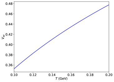
Figure 1: (Color online) Left: Number density as a function of temperature. Right: Average velocity of $D$ meson as a function of temperature.

In this section, we have numerically studied the influence of rotation on the spatial diffusion of $D$ mesons in hadronic matter using the IHRG model, which comprises all the non-interacting hadrons and their resonances up to mass 2.6 GeV as listed in Ref. [71]. To understand the rotational effect, we have investigated the results of $D$ meson diffusion coefficients in a rotating medium of hadrons and compared them with those when the medium was not rotating. We have used the RTA to calculate the diffusion coefficient, which is defined as the ratio of conductivity to susceptibility, referring to Eq. (16). The relaxation time of the $D$ meson depends on its velocity and the system’s number density as described in Eq. (22).

The temperature-dependent number density profile of the HRG system and the temperature variation of the $D$ meson velocity are presented in the left and right panels of Fig. 1, respectively. Our numerical estimation suggests that the average velocity of $D$ mesons within the hadron gas medium increases with $T$ in the hadronic temperature domain (up to 0.2 GeV), ranging from 0.35 to 0.47. As observed in the left panel of Fig. 1, the reader can guess a $T^{b}$-dependence (with $b>3$) of the actual number density of HRG, and hence, a $T^{-b}$-dependence of relaxation time can be expected as shown in the left panel of Fig. 2. The scattering length $a$ is an important parameter for estimating $\tau_{c}$. Here, we have taken $a=0.18$ and $0.85$ fm to analyze the variation on the order of magnitude of $\tau_{c}$.

Figure 2: (Color online) Left: Relaxation time of $D$ meson as a function of temperature. Right: spatial diffusion coefficient ($D$) for $D$ meson as a function of temperature and comparing the result with Ozvenchuk et al. [68], Ghosh et al.[69], He et al.[113], Torres-Rincon et al.[114], and Goswami et al.[115]

In the left panel of Fig. 2, we have presented the temperature-dependent relaxation time ($\tau_{c}$) depicted within the hadronic region using the hard sphere scattering model. As described in Eq. 22 of Sec. II.2, $\tau_{c}$ is inversely proportional to number density, velocity, and scattering length. Using two different scattering lengths: $a$=0.18 fm and $a$=0.85 fm (the reason for choosing these two specific values of $a$ will be clear later), we have shown the results that the relaxation time decreases as the temperature increases, consistent with expectations in a thermally evolving system. At a particular temperature, the relaxation time exhibits a sharp decrease as the scattering length increases, suggesting stronger particle interactions.

In the right panel of Fig. 2 we have illustrated the temperature dependence of the scaled diffusion coefficient ($2\pi TD$). The figure shows that $2\pi TD$ decreases as the temperature increases, which gives a similar nature to the earlier spatial diffusion data from Ghosh et al. [69] (open black circles), Ozvenchuk et al. [68] (solid purple stars), He et al.[113] (open blue diamond), Torres-Rincon et al.[114] (green square), and Goswami et al.[115] (red cross). To cover these earlier estimations, we have taken two different values of the scattering length, $a=0.18$ fm and $0.85$ fm, for the computation of $D^{||}\equiv D$ from Eq. 18. Furthermore, the figure also demonstrates that as the scattering length increases, the value of $2\pi TD$ decreases further, indicating that a lower diffusion coefficient results from stronger particle interactions. After tuning the relaxation time (by tuning $a$) to cover the earlier estimation of the diffusion coefficient in the absence of the rotation, we will now proceed to show the variation of perpendicular and hall conductivity and diffusion coefficients as a function of $\Omega$ and $T$.

Figure 3: (Color online) Left: Parallel, perpendicular and Hall conductivity of $D$ meson ($\sigma/T$, $\sigma^{\perp}/T$, $\sigma^{\times}/T$) as functions of temperature. Right: Parallel, perpendicular, and Hall spatial diffusion coefficients ($2\pi TD$, $2\pi TD^{\perp}$, $2\pi TD^{\times}$) as functions of temperature for $D$ meson.

We have presented the temperature dependence of the scaled conductivity component of $D$ mesons in the left panel of Fig. 3: the parallel ($\sigma$ / $T$, represented by the blue solid line), perpendicular ($\sigma^{\perp}$ / $T$, represented by the red dashed line) and Hall ($\sigma^{\times}$ / $T$, represented by the black dotted line) conductivities. These components are evaluated at a constant hard-sphere scattering length of $a=0.85$ fm and a rotational time scale of $\tau_{\Omega}=5$ fm (corresponding to $\Omega$ = 0.02 GeV). The parallel conductivity remains unchanged under rotation, while the perpendicular and Hall conductivities are affected by the rotational conditions. These calculations are performed using the framework discussed in Eq. [13- 15], in Sec. II.1. It can be noted that in the temperature region, $T\in(0.1,0.15)$ GeV, all three components of conductivity increase.

In the right panel of Fig. 3, the temperature dependence of the diffusion components of $D$ meson, i.e. parallel ($2\pi TD$), perpendicular ($2\pi TD^{\perp}$) and Hall ($2\pi TD^{\times}$) are shown at a constant value of a = 0.85 fm and $\tau_{\Omega}=5fm$. Referring to Eq. 18, 19, and 20 — it becomes evident that rotation does not affect the susceptibility ($\chi$); only the conductivity is modified. Here, we find that $2\pi TD$ remains approximately equal to $2\pi TD^{\perp}$ for temperatures $T\geq 0.17$ GeV.

Figure 4: (Color online) Left: Perpendicular and Hall conductivity of $D$ meson ($\sigma^{\perp}$ / $\sigma$ , $\sigma^{\times}$ / $\sigma$) as functions of ${\Omega}$. Right: Perpendicular and Hall spatial diffusion coefficients of $D$ meson ($D^{\perp}$ / $D$, $D^{\times}$ / $D$) as functions of ${\Omega}$ .

The left panel of Fig. 4 shows the variation of perpendicular and hall components (normalized) of conductivity with angular velocity $\Omega$. In the absence of rotation, that is, when $\Omega=0$, $\sigma^{\perp}/\sigma=1$ and $\sigma^{\times}/\sigma=0$. The right panel of Fig. 4, shows the variation of perpendicular ($D^{\perp}$) and hall ($D^{\times}$) diffusion coefficients normalized with spatial diffusion coefficient with angular velocity $\Omega$. As we have taken the ratio of the diffusion components in this case, therefore we are getting a full resemblance with the left panel of the figure 4. By comparing the right panel of Fig. 3 with Fig. 4, we can conclude that high temperatures affect the diffusion coefficient in a manner similar to low rotations ($\Omega\to 0$).

Figure 5: (Color online) Percentage deviation of $R_{AA}$ of $D$ meson as a function of ${\Omega}$ .

After the general discussions on the diffusion coefficients of $D$ meson and its dependence on $\Omega$ and $T$, we will now proceed to predict some phenomenological consequences of the $D$ meson diffusion in rotating HRG matter. Let us see how the rotation or Coriolis force impacts the nuclear modification factor $R_{AA}$ of $D$ mesons, an essential observable in relativistic heavy ion collisions. Here, we will adopt a crude and approximated expression $R_{AA}\sim e^{-\gamma\Delta t}$ [67], where $\Delta t$ denotes the duration of the hadronic phase, taken to be 5 fm, and $\gamma=\frac{1}{\tau_{c}}$ is the inverse of the $D$ meson relaxation time. Thus, we have $R_{AA}(\Omega)\sim e^{-\Delta t/\tau_{c}^{\perp}}$ and $R_{AA}(\Omega=0)\sim e^{-\Delta t/\tau_{c}}$, where we have used $\tau_{c}^{\perp}$ as an effective relaxation time in the presence of rotation. In Fig. 5, we illustrate the suppression of $D$ mesons as a function of the angular velocity $\Omega$. The average angular velocity $\Omega$ of nuclear matter produced in HIC is maximum in the QGP phase and decreases with time as the medium expands into hadron gas. For the appropriate value of the angular velocity $\Omega$ in the hadronic phase, we have considered the range $0.0028-0.0078\rm{~{}fm}^{-1}$, as indicated in Fig.(11) of Ref. [116]. With the effect of rotation, the percentage deviation in $R_{AA}$ can be defined as:

$$\dfrac{\Delta R_{AA}}{R_{AA}}=\dfrac{e^{-\Delta t/\tau_{c}^{\perp}}-e^{-\Delta t/\tau_{c}}}{e^{-\Delta t/\tau_{c}}}\times 100\%.$$

This expression quantifies the change in the nuclear modification factor due to the influence of rotation via the Coriolis force. From the analysis of the figure, we observe that the percentage deviation in the nuclear modification factor is negative, suggesting that for finite $\Omega$, the $R_{AA}$ of the $D$ meson is further suppressed. Furthermore, our calculations for the hadronic phase $\Omega$ show that $\left|\dfrac{\Delta R_{AA}}{R_{AA}}\right|\lesssim 20\%$ for rotating $D$ mesons, highlighting the significant influence of rotation on the transport properties within the hadronic phase. Readers should consider this ${\Delta R_{AA}}$ estimation due to Coriolis force as a gross measurement, which concludes that a non-zero and non-negligible impact of Coriolis force on $D$ meson diffusion may be hidden in actual ${R_{AA}}$ data. The actual 3-dimensional picture at finite rotation and realistic connection of ${R_{AA}}$ with the $D$ meson diffusion coefficients components will be a little complicated but very interesting for future research. If we assume ’z’ as a beam axis of heavy ion collision experiments, then ’y’ will be the direction of angular momentum direction or parallel component ($D^{||}$) of $D$ meson diffusion, ’x’ will be its perpendicular component ($D^{\perp}$). Our calculations suggest that finite rotation of medium via Coriolis force will create an anisotropic diffusion (as $D^{||}>D^{\perp}$) and Hall diffusion ($D^{\times}$), which can have a role in the overall modification of $R_{AA}$ due to finite rotation. Present work has projected a simple modification of $R_{AA}$ along perpendicular direction only via $D^{\perp}$ but to connect with experimental group $R_{AA}$ data, one has to consider detailed diffusion matrix at finite rotation and formulate them with phenomenological quantity $R_{AA}$, which is at present missing in literature. We are planning to explore it in the near future.

IV Summary

In this work, we calculate the diffusion coefficients of $D$ mesons diffusing through the background of a rotating hadron gas. To derive the expressions for these diffusion coefficients, we first formulate a relaxation time-approximated Boltzmann transport equation in a rotating frame. We model the background hadron gas using the hadron resonance gas model and determine the relaxation time for the interactions of $D$ meson with the hadron resonance gas using the hard sphere scattering interactions. We treat the scattering length as a free parameter to adjust the relaxation time. To obtain the diffusion coefficients of $D$ meson, we first calculate its conductivity by employing the Boltzmann transport equation. We then relate the diffusion of heavy mesons to their conductivity according to Einstein’s diffusion relation, which states that the diffusion coefficients are the ratio of conductivity to susceptibility. The Coriolis force present in the force term of the Boltzmann transport equation is the cause of the anisotropic nature of diffusion of $D$ meson. This anisotropy in the meson diffusion tensor caused by the Coriolis force in rotating frames is similar to that observed in systems influenced by the Lorentz force in magnetic fields. The tensor structure of both the meson conductivity and diffusion are similar and can be encoded in three components: the parallel, perpendicular, and Hall. The parallel component is independent of angular velocity ($\Omega$) and is equal to the conductivity or diffusion in the absence of rotation. Due to the finite rotation of the medium, parallel and perpendicular diffusion or conductivity components become different. So, anisotropic conductivity or diffusion matrices will be produced at finite rotation via this Coriolis force. Along with the anisotropic structure of diffusion or conduction, a new directional Hall component is induced completely due to the finite rotation of the medium, as it was absent in the non-rotating scenario. To accurately depict the diffusion coefficients, we first adjusted the relaxation time by tuning the scattering length from $0.18$ fm to $0.85$ fm, aligning with previous estimates of diffusion coefficients for a medium with $\Omega=0$. Following this calibration, we examined the variations of normalized parallel, perpendicular, and Hall conductivity (normalized by $T$), as well as diffusion coefficients (multiplied by $2\pi T$), as functions of temperature and angular velocity of the HRG, setting $\tau_{c}$ corresponding to $a=0.85$ fm. We have noticed that the anisotropic nature, where parallel and perpendicular components become different in magnitude, and a non-zero Hall component of $D$ meson diffusion or conductivity becomes prominent, pertains to the low temperature and high angular velocity regime. So, an isotropic conductivity or diffusion tensor of $D$ meson with negligible Hall coefficient can be expected in high temperature and low angular velocity domains.

Next, we have focused on the phenomenological range of temperature and angular velocity, which can be covered by peripheral collision of RHIC or LHC experiments. We have used an approximate relation between perpendicular diffusion or relaxation time and the phenomenological quantity - nuclear suppression factor $R_{AA}$ of $D$ meson. Our findings indicate that $R_{AA}$ becomes further suppressed as angular velocity increases, with a maximum percentage deviation of approximately $20\%$ for rotating $D$ meson. This underscores the significant role of rotation in modifying the transport dynamics within the hadronic phase, providing valuable insights for future studies on heavy-ion collisions.

V Acknowledgement

NP and AD gratefully acknowledge the Ministry of Education (MoE), Govt. of India. AD thanks Dani Rose J Marattukalam for valuable discussions.

Appendix A HEAVY MESON CONDUCTIVITY FROM RELATIVISTIC BOLTZMANN EQUATION

In this appendix, we will provide the derivation of Eq. (11) and Eq. (12) with the help of BTE. Substituting $f=f^{0}+\delta f$ we can rewrite Eq. (9) as follows:

$$p^{\mu}\frac{\partial f^{0}}{\partial x^{\mu}}-\Gamma_{\mu\lambda}^{\alpha}p^{\mu}p^{\lambda}\frac{\partial f^{0}+\delta f}{\partial p^{\alpha}}=-(u^{\alpha}p_{\alpha})\frac{\delta f}{\tau_{c}}$$

$$\implies -f^{0}(1+f^{0})\bigg{[}\frac{p^{\mu}p^{\alpha}}{T}(\partial_{\mu}u_{\alpha}-\Gamma^{\sigma}_{\mu\alpha}u_{\sigma})+p^{\mu}(u^{\alpha}p_{\alpha})\partial_{\mu}\left(\frac{1}{T}\right)-p^{\mu}\partial_{\mu}\left(\frac{\mu_{D}}{T}\right)\bigg{]}$$

$$-\Gamma^{\sigma}_{\mu\lambda}p^{\mu}p^{\lambda}\frac{\partial\delta f}{\partial p^{\sigma}}=-(u^{\alpha}p_{\alpha})\frac{\delta f}{\tau_{c}}$$

$$\implies -f^{0}(1+f^{0})\bigg{[}\frac{p_{0}}{\sqrt{g_{00}}}p^{0}\partial_{0}\left(\frac{1}{T}\right)+\frac{p_{0}}{\sqrt{g_{00}}}p^{i}\nabla_{i}\left(\frac{1}{T}\right)-p^{0}\partial_{0}\left(\frac{\mu_{D}}{T}\right)-p^{i}\nabla_{i}\left(\frac{\mu_{D}}{T}\right)\bigg{]}$$

$$+2p_{0}(\vec{p}\times\vec{\Omega})\cdot\frac{\partial\delta f}{\partial\vec{p}}=-\frac{p_{0}}{\sqrt{g_{00}}}\frac{\delta f}{\tau_{c}},$$

$$\implies -f^{0}(1+f^{0})\bigg{[}\frac{1}{T^{2}}\frac{p^{i}}{E}(\mu_{D}-E)\nabla_{i}T-\frac{p^{i}}{ET}\nabla_{i}\mu_{D}\bigg{]}+2(\vec{p}\times\vec{\Omega})\cdot\frac{\partial\delta f}{\partial\vec{p}}=-\frac{\delta f}{\tau_{c}},$$ (24)

where we implicitly assumed that the Greek indices run from $0\text{ to }4$ and Latin index $i$ run from $0\text{ to }3$; also, we defined $p_{0}\equiv E$. In the simplification process of obtaining Eq. (24) from Eq. (9), we used the following approximations: the terms which are 1st order in $\Omega x$, $\Omega y$, and $\frac{\Omega}{T}$ have been retained and the time derivatives of $\mu_{D}$ and $T$ have been ignored assuming a steady state condition [66]. In Eq. (24) keeping only the thermodynamic force $\partial_{i}\mu$, which is responsible for diffusion we have,

$$-\frac{\partial f^{0}}{\partial E}\frac{p^{i}}{E}\nabla_{i}\mu+2(\vec{p}\times\vec{\Omega})\cdot\frac{\partial\delta f}{\partial\vec{p}}=-\frac{\delta f}{\tau_{c}}.$$ (25)

For the calculation of current density $J^{i}$, we have to solve Eq. (25) for $\delta f$. A glance at Eq. (25) suggest that the solution $\delta f$ should have the following form: $\delta f=-\vec{p}\cdot\vec{X}\frac{\partial f^{0}}{\partial E}$, where $\vec{X}$ is an arbitrary vector. The vector $\vec{X}$ can be decomposed in terms of the available basis vector at our hand, $\hat{\mu}_{D}=\frac{-\vec{\nabla}\mu_{D}}{||\vec{\nabla}\mu_{D}||}$, $\hat{\omega}\equiv\frac{\vec{\Omega}}{||\vec{\Omega}||}$, and $\hat{\mu}_{D}\times\hat{\omega}$ as: $\vec{X}=\alpha\hat{\mu}_{D}+\beta\hat{\omega}+\gamma(\hat{\mu}_{D}\times\hat{\omega})$ with the unknowns $\alpha$, $\beta$, and $\gamma$. Therefore, the final task boils down to determining the unknowns $\alpha$, $\beta$, and $\gamma$ by substituting $\delta f$ in Eq. (25 )as follows:

$$\frac{\partial f^{0}}{\partial E}\frac{\vec{p}}{E}\cdot(-\vec{\nabla}\mu_{D})+2(\vec{p}\times\vec{\Omega})\cdot\frac{\partial}{\partial\vec{p}}\left(-\vec{p}\cdot\vec{X}\frac{\partial f^{0}}{\partial E}\right)=\frac{\vec{p}\cdot\vec{X}}{\tau_{c}}\frac{\partial f^{0}}{\partial E}$$

$$\implies \frac{\partial f^{0}}{\partial E}\frac{\vec{p}}{E}\cdot(-\vec{\nabla}\mu_{D})-2(\vec{p}\times\vec{\Omega})\cdot\vec{X}\frac{\partial f}{\partial E}=\frac{\vec{p}\cdot\vec{X}}{\tau_{c}}\frac{\partial f^{0}}{\partial E}$$

$$\implies \frac{\partial f^{0}}{\partial E}\vec{p}\cdot\bigg{[}-\frac{1}{E}\vec{\nabla}\mu_{D}-2(\vec{\Omega}\times\vec{X})\bigg{]}=\frac{\vec{X}}{\tau_{c}}\frac{\partial f^{0}}{\partial E}\cdot\vec{p}$$

$$\implies -\frac{1}{E}\vec{\nabla}\mu_{D}-2(\vec{\Omega}\times\vec{X})=\frac{X}{\tau_{c}}.$$ (26)

Substituting the result $2(\vec{X}\times\vec{\Omega})=(\alpha\hat{\mu}_{D}+\beta\hat{\omega}+\gamma(\hat{\mu}_{D}\times\hat{\omega}))\times\Omega\hat{\omega}=2\alpha\Omega(\hat{\mu}_{D}\times\hat{\omega})-2\gamma\Omega\hat{\mu}_{D}+2\gamma\Omega(\hat{\mu}_{D}\cdot\hat{\omega})\hat{\omega}$, in Eq. (26) we have,

$$\left(\frac{||\vec{\nabla}\mu_{D}||}{E}-\frac{\gamma}{\tau_{\Omega}}\right)\hat{\mu}_{D}+\frac{\gamma}{\tau_{\Omega}}(\hat{\mu}_{D}\cdot\hat{\omega})\hat{\omega}+\frac{\alpha}{\tau_{\Omega}}(\hat{\mu}_{D}\times\hat{\omega})=\frac{\alpha}{\tau_{c}}\hat{\mu}_{D}+\frac{\beta}{\tau_{c}}\hat{\omega}+\frac{\gamma}{\tau_{c}}(\hat{\mu}_{D}\times\hat{\omega}),$$ (27)

where we defined $\tau_{\Omega}\equiv\frac{1}{2\Omega}$. Simplifying Eq. (27), one obtain the following expressions for the unknowns $\alpha$, $\beta$ and $\gamma$,

$$\alpha =\frac{||\vec{\nabla}\mu_{D}||}{E}\frac{\tau_{c}}{1+\big{(}\frac{\tau_{c}}{\tau_{\Omega}}\big{)}^{2}}, \beta =\left(\frac{\tau_{c}}{\tau_{\Omega}}\right)^{2}(\hat{\omega}\cdot\hat{\mu}_{D})\frac{||\vec{\nabla}\mu_{D}||}{E}\frac{\tau_{c}}{1+\big{(}\frac{\tau_{c}}{\tau_{\Omega}}\big{)}^{2}}, \gamma =\left(\frac{\tau_{c}}{\tau_{\Omega}}\right)\frac{||\vec{\nabla}\mu_{D}||}{E}\frac{\tau_{c}}{1+\big{(}\frac{\tau_{c}}{\tau_{\Omega}}\big{)}^{2}}.$$

The $\delta f$ upon substitution of $\alpha$, $\beta$ and $\gamma$ becomes,

$$\delta f = -p^{j}X^{j}\frac{\partial f^{0}}{\partial E}$$ (28)

$$= -\frac{\partial f^{0}}{\partial E}p^{j}(\alpha\hat{\mu}_{D}^{j}+\beta\omega^{j}+\gamma(\hat{\mu}_{D}\times\hat{\omega})^{j})$$

$$= -\frac{\partial f^{0}}{\partial E}p^{j}(\alpha\hat{\mu}_{D}^{j}+\beta\omega^{j}+\gamma\epsilon^{jkl}\hat{\mu}_{D}^{k}\omega^{l})$$

$$= -\frac{\partial f^{0}}{\partial E}\frac{\tau_{c}}{1+\big{(}\frac{\tau_{c}}{\tau_{\Omega}}\big{)}^{2}}\frac{p^{j}}{E}\bigg{[}||\vec{\nabla}\mu_{D}||\hat{\mu}_{D}^{j}+\left(\frac{\tau_{c}}{\tau_{\Omega}}\right)^{2}\omega^{j}\omega^{k}\hat{\mu}_{D}^{k}||\vec{\nabla}\mu_{D}||+\frac{\tau_{c}}{\tau_{\Omega}}||\vec{\nabla}\mu_{D}||\epsilon^{jkl}\hat{\mu}_{D}^{k}\omega^{l}\bigg{]}$$

$$= -\frac{\partial f^{0}}{\partial E}\frac{p^{j}}{E}\frac{\tau_{c}}{1+\big{(}\frac{\tau_{c}}{\tau_{\Omega}}\big{)}^{2}}\bigg{[}\delta^{ij}+\frac{\tau_{c}}{\tau_{\Omega}}\epsilon^{jik}\omega^{k}+\left(\frac{\tau_{c}}{\tau_{\Omega}}\right)^{2}\omega^{i}\omega^{j}\bigg{]}(-\nabla_{i}\mu_{D})$$

The current density $J^{i}$ can now be expressed as,

$$J^{i} = \int\frac{d^{3}\vec{p}}{(2\pi)^{3}}\frac{p^{i}}{E}\delta f$$ (29)

$$= \int\frac{d^{3}\vec{p}}{(2\pi)^{3}}\frac{p^{i}p^{j}}{E^{2}}\left(-\frac{\partial f^{0}}{\partial E}\right)\frac{\tau_{c}}{1+\big{(}\frac{\tau_{c}}{\tau_{\Omega}}\big{)}^{2}}(-\nabla_{k}\mu_{D})\bigg{[}\delta^{kj}+\frac{\tau_{c}}{\tau_{\Omega}}\epsilon^{jkl}\omega^{l}+\left(\frac{\tau_{c}}{\tau_{\Omega}}\right)^{2}\omega^{k}\omega^{j}\bigg{]}$$

$$= \int\frac{d^{3}p}{(2\pi)^{3}}\frac{p^{2}}{3E^{2}}\delta^{ij}\left(-\frac{\partial f^{0}}{\partial E}\right)\frac{\tau_{c}}{1+\big{(}\frac{\tau_{c}}{\tau_{\Omega}}\big{)}^{2}}(-\nabla_{k}\mu_{D})\bigg{[}\delta^{kj}+\frac{\tau_{c}}{\tau_{\Omega}}\epsilon^{jkl}\omega^{l}+\left(\frac{\tau_{c}}{\tau_{\Omega}}\right)^{2}\omega^{k}\omega^{j}\bigg{]},(d^{3}p\equiv 4\pi p^{2}dp)$$

$$= \int\frac{d^{3}p}{(2\pi)^{3}}\frac{p^{2}}{3E^{2}}\left(-\frac{\partial f^{0}}{\partial E}\right)\frac{\tau_{c}}{1+\big{(}\frac{\tau_{c}}{\tau_{\Omega}}\big{)}^{2}}(-\nabla_{k}\mu_{D})\bigg{[}\delta^{ki}+\frac{\tau_{c}}{\tau_{\Omega}}\epsilon^{ikl}\omega^{l}+\left(\frac{\tau_{c}}{\tau_{\Omega}}\right)^{2}\omega^{k}\omega^{i}\bigg{]}$$

$$= \frac{1}{T}\int\frac{d^{3}p}{(2\pi)^{3}}\frac{p^{2}}{3E^{2}}\frac{\tau_{c}}{1+\big{(}\frac{\tau_{c}}{\tau_{\Omega}}\big{)}^{2}}(-\nabla_{j}\mu_{D})\bigg{[}\delta^{ij}+\frac{\tau_{c}}{\tau_{\Omega}}\epsilon^{ijk}\omega^{k}+\left(\frac{\tau_{c}}{\tau_{\Omega}}\right)^{2}\omega^{i}\omega^{j}\bigg{]}f^{0}(1+f^{0})$$

Comparing it with Eq. (2) we obtain the conductivity matrix as follows:

$$\sigma^{ij}=\sigma^{0}\delta^{ij}+\sigma^{1}\epsilon^{ijk}\omega^{k}+\sigma^{2}\omega^{i}\omega^{j},$$ (30)

where $\sigma^{n}$ are expressed as,

$$\sigma^{n}=\frac{1}{T}\int\frac{d^{3}p}{(2\pi)^{3}}\frac{p^{2}}{3E^{2}}f^{0}(1+f^{0})\frac{\tau_{c}(\tau_{c}/\tau_{\Omega})^{n}}{1+(\tau_{c}/\tau_{\Omega})^{2}}$$ (31)

References

- Shuryak [2005] E. V. Shuryak, What RHIC experiments and theory tell us about properties of quark-gluon plasma?, Nucl. Phys. A 750, 64 (2005), arXiv:hep-ph/0405066 .
- Wong [1995] C. Y. Wong, Introduction to high-energy heavy ion collisions (1995).
- Gossiaux and Aichelin [2008] P. B. Gossiaux and J. Aichelin, Toward an understanding of the single electron data measured at the bnl relativistic heavy ion collider (rhic), Phys. Rev. C 78, 014904 (2008).
- Gossiaux et al. [2009] P. B. Gossiaux, R. Bierkandt, and J. Aichelin, Tomography of quark gluon plasma at energies available at the bnl relativistic heavy ion collider (rhic) and the cern large hadron collider (lhc), Physical Review C 79, 10.1103/physrevc.79.044906 (2009).
- Gossiaux and Aichelin [2009a] P. B. Gossiaux and J. Aichelin, Tomography of the quark–gluon plasma by heavy quarks, Journal of Physics G: Nuclear and Particle Physics 36, 064028 (2009a).
- Nahrgang et al. [2015a] M. Nahrgang, J. Aichelin, S. Bass, P. B. Gossiaux, and K. Werner, Elliptic and triangular flow of heavy flavor in heavy-ion collisions, Physical Review C 91, 10.1103/physrevc.91.014904 (2015a).
- Das et al. [2015] S. K. Das, F. Scardina, S. Plumari, and V. Greco, Toward a solution to the raa and v2 puzzle for heavy quarks, Physics Letters B 747, 260 (2015).
- Scardina et al. [2017] F. Scardina, S. K. Das, V. Minissale, S. Plumari, and V. Greco, Estimating the charm quark diffusion coefficient and thermalization time from meson spectra at energies available at the bnl relativistic heavy ion collider and the cern large hadron collider, Phys. Rev. C 96, 044905 (2017).
- Chandra and Das [2024] V. Chandra and S. K. Das, B-mesons as essential probes of hot QCD matter, Eur. Phys. J. ST 233, 429 (2024), arXiv:2402.18870 [hep-ph] .
- Pooja et al. [2023a] Pooja, S. K. Das, V. Greco, and M. Ruggieri, Thermalization and isotropization of heavy quarks in a non-Markovian medium in high-energy nuclear collisions, Phys. Rev. D 108, 054026 (2023a), arXiv:2306.13749 [hep-ph] .
- Prakash et al. [2023] J. Prakash, V. Chandra, and S. K. Das, Heavy quark radiation in an anisotropic hot QCD medium, Phys. Rev. D 108, 096016 (2023), arXiv:2306.07966 [hep-ph] .
- Thoma [1991] M. H. Thoma, Collisional energy loss of high-energy jets in the quark gluon plasma, Phys. Lett. B 273, 128 (1991).
- Mustafa et al. [1998] M. G. Mustafa, D. Pal, D. K. Srivastava, and M. Thoma, Radiative energy loss of heavy quarks in a quark gluon plasma, Phys. Lett. B 428, 234 (1998), arXiv:nucl-th/9711059 .
- Gossiaux and Aichelin [2009b] P. Gossiaux and J. Aichelin, Energy loss of heavy quarks in a qgp with a running coupling constant approach, Nuclear Physics A 830, 203c–206c (2009b).
- Gossiaux et al. [2010] P. B. Gossiaux, J. Aichelin, T. Gousset, and V. Guiho, Competition of heavy quark radiative and collisional energy loss in deconfined matter, Journal of Physics G: Nuclear and Particle Physics 37, 094019 (2010).
- Kumar et al. [2022] A. Kumar, M. Kurian, S. K. Das, and V. Chandra, Drag of heavy quarks in an anisotropic QCD medium beyond the static limit, Phys. Rev. C 105, 054903 (2022), arXiv:2111.07563 [hep-ph] .
- Ruggieri et al. [2022] M. Ruggieri, Pooja, J. Prakash, and S. K. Das, Memory effects on energy loss and diffusion of heavy quarks in the quark-gluon plasma, Phys. Rev. D 106, 034032 (2022), arXiv:2203.06712 [hep-ph] .
- Prakash et al. [2021] J. Prakash, M. Kurian, S. K. Das, and V. Chandra, Heavy quark transport in an anisotropic hot QCD medium: Collisional and Radiative processes, Phys. Rev. D 103, 094009 (2021), arXiv:2102.07082 [hep-ph] .
- Acharya et al. [2022] S. Acharya et al. (ALICE), Prompt D0, D+, and D∗+ production in Pb–Pb collisions at = 5.02 TeV, JHEP 01, 174, arXiv:2110.09420 [nucl-ex] .
- Prino and Rapp [2016] F. Prino and R. Rapp, Open Heavy Flavor in QCD Matter and in Nuclear Collisions, J. Phys. G 43, 093002 (2016), arXiv:1603.00529 [nucl-ex] .
- Beraudo et al. [2018] A. Beraudo et al., Extraction of Heavy-Flavor Transport Coefficients in QCD Matter, Nucl. Phys. A 979, 21 (2018), arXiv:1803.03824 [nucl-th] .
- Das et al. [2010] S. K. Das, J.-e. Alam, and P. Mohanty, Dragging Heavy Quarks in Quark Gluon Plasma at the Large Hadron Collider, Phys. Rev. C 82, 014908 (2010), arXiv:1003.5508 [nucl-th] .
- Cao et al. [2019] S. Cao, G. Coci, S. K. Das, W. Ke, S. Y. F. Liu, S. Plumari, T. Song, Y. Xu, J. Aichelin, S. Bass, E. Bratkovskaya, X. Dong, P. B. Gossiaux, V. Greco, M. He, M. Nahrgang, R. Rapp, F. Scardina, and X.-N. Wang, Toward the determination of heavy-quark transport coefficients in quark-gluon plasma, Physical Review C 99, 10.1103/physrevc.99.054907 (2019).
- Zhao et al. [2023] J. Zhao, J. Aichelin, P. B. Gossiaux, A. Beraudo, S. Cao, W. Fan, M. He, V. Minissale, T. Song, I. Vitev, R. Rapp, S. Bass, E. Bratkovskaya, V. Greco, and S. Plumari, Hadronization of heavy quarks (2023), arXiv:2311.10621 [hep-ph] .
- Boguslavski et al. [2020] K. Boguslavski, A. Kurkela, T. Lappi, and J. Peuron, Heavy quark diffusion in an overoccupied gluon plasma, JHEP 09, 077, arXiv:2005.02418 [hep-ph] .
- Boguslavski et al. [2024] K. Boguslavski, A. Kurkela, T. Lappi, F. Lindenbauer, and J. Peuron, Heavy quark diffusion coefficient in heavy-ion collisions via kinetic theory, Phys. Rev. D 109, 014025 (2024), arXiv:2303.12520 [hep-ph] .
- Pooja et al. [2024] Pooja, M. Y. Jamal, P. P. Bhaduri, M. Ruggieri, and S. K. Das, cc¯ and bb¯ suppression in the glasma, Phys. Rev. D 110, 094018 (2024), arXiv:2404.05315 [hep-ph] .
- Pooja et al. [2023b] Pooja, S. K. Das, V. Greco, and M. Ruggieri, Anisotropic fluctuations of angular momentum of heavy quarks in the Glasma, Eur. Phys. J. Plus 138, 313 (2023b), arXiv:2212.09725 [hep-ph] .
- Backfried et al. [2024] L. Backfried, K. Boguslavski, and P. Hotzy, Heavy-quark diffusion in 2+1D and Glasma-like plasmas: evidence of a transport peak, (2024), arXiv:2408.12646 [hep-ph] .
- Tuchin [2013] K. Tuchin, Particle production in strong electromagnetic fields in relativistic heavy-ion collisions, Adv. High Energy Phys. 2013, 490495 (2013), arXiv:1301.0099 [hep-ph] .
- Skokov et al. [2009] V. Skokov, A. Y. Illarionov, and V. Toneev, Estimate of the magnetic field strength in heavy-ion collisions, Int. J. Mod. Phys. A 24, 5925 (2009), arXiv:0907.1396 [nucl-th] .
- Bzdak and Skokov [2012] A. Bzdak and V. Skokov, Event-by-event fluctuations of magnetic and electric fields in heavy ion collisions, Phys. Lett. B 710, 171 (2012), arXiv:1111.1949 [hep-ph] .
- Das et al. [2017] S. K. Das, S. Plumari, S. Chatterjee, J. Alam, F. Scardina, and V. Greco, Directed Flow of Charm Quarks as a Witness of the Initial Strong Magnetic Field in Ultra-Relativistic Heavy Ion Collisions, Phys. Lett. B 768, 260 (2017), arXiv:1608.02231 [nucl-th] .
- Banerjee et al. [2023] D. Banerjee, P. Das, S. Paul, A. Modak, A. Budhraja, S. Ghosh, and S. K. Prasad, Effect of magnetic field on jet transport coefficient , Pramana 97, 206 (2023), arXiv:2103.14440 [hep-ph] .
- Satapathy et al. [2024] S. Satapathy, S. De, J. Dey, and S. Ghosh, Spatial diffusion of quarks in a background magnetic field, Phys. Rev. C 109, 024904 (2024), arXiv:2212.08933 [hep-ph] .
- Liang and Wang [2005] Z.-T. Liang and X.-N. Wang, Globally polarized quark-gluon plasma in non-central A+A collisions, Phys. Rev. Lett. 94, 102301 (2005), [Erratum: Phys.Rev.Lett. 96, 039901 (2006)], arXiv:nucl-th/0410079 .
- Becattini et al. [2008] F. Becattini, F. Piccinini, and J. Rizzo, Angular momentum conservation in heavy ion collisions at very high energy, Phys. Rev. C 77, 024906 (2008), arXiv:0711.1253 [nucl-th] .
- Adamczyk et al. [2017] L. Adamczyk et al. (STAR), Global hyperon polarization in nuclear collisions: evidence for the most vortical fluid, Nature 548, 62 (2017), arXiv:1701.06657 [nucl-ex] .
- Becattini et al. [2013] F. Becattini, V. Chandra, L. Del Zanna, and E. Grossi, Relativistic distribution function for particles with spin at local thermodynamical equilibrium, Annals of Physics 338, 32 (2013).
- Son and Surówka [2009] D. T. Son and P. Surówka, Hydrodynamics with triangle anomalies, Phys. Rev. Lett. 103, 191601 (2009).
- Adam et al. [2018] J. Adam et al. (STAR), Global polarization of hyperons in Au+Au collisions at = 200 GeV, Phys. Rev. C 98, 014910 (2018), arXiv:1805.04400 [nucl-ex] .
- Acharya et al. [2020] S. Acharya et al. (ALICE), Evidence of Spin-Orbital Angular Momentum Interactions in Relativistic Heavy-Ion Collisions, Phys. Rev. Lett. 125, 012301 (2020), arXiv:1910.14408 [nucl-ex] .
- Abdallah et al. [2023] M. S. Abdallah et al. (STAR), Pattern of global spin alignment of and K∗0 mesons in heavy-ion collisions, Nature 614, 244 (2023), arXiv:2204.02302 [hep-ph] .
- Acharya et al. [2023] S. Acharya et al. (ALICE), Measurement of the J/ Polarization with Respect to the Event Plane in Pb-Pb Collisions at the LHC, Phys. Rev. Lett. 131, 042303 (2023), arXiv:2204.10171 [nucl-ex] .
- Sivardiere [1983] J. Sivardiere, On the analogy between inertial and electromagnetic forces, European Journal of Physics 4, 162 (1983).
- Johnson [2000] B. L. Johnson, Inertial forces and the hall effect, Am. J. Phys. 68, 649 (2000).
- Sakurai [1980] J. J. Sakurai, Comments on quantum-mechanical interference due to the earth’s rotation, Phys. Rev. D 21, 2993 (1980).
- Dey et al. [2021a] J. Dey, S. Satapathy, P. Murmu, and S. Ghosh, Shear viscosity and electrical conductivity of the relativistic fluid in the presence of a magnetic field: A massless case, Pramana 95, 125 (2021a), arXiv:1907.11164 [hep-ph] .
- Dash et al. [2020] A. Dash, S. Samanta, J. Dey, U. Gangopadhyaya, S. Ghosh, and V. Roy, Anisotropic transport properties of a hadron resonance gas in a magnetic field, Phys. Rev. D 102, 016016 (2020), arXiv:2002.08781 [nucl-th] .
- Dey et al. [2022] J. Dey, S. Samanta, S. Ghosh, and S. Satapathy, Quantum expression for the electrical conductivity of massless quark matter and of the hadron resonance gas in the presence of a magnetic field, Phys. Rev. C 106, 044914 (2022), arXiv:2002.04434 [nucl-th] .
- Ghosh et al. [2020] S. Ghosh, A. Bandyopadhyay, R. L. S. Farias, J. Dey, and G. a. Krein, Anisotropic electrical conductivity of magnetized hot quark matter, Phys. Rev. D 102, 114015 (2020), arXiv:1911.10005 [hep-ph] .
- Dey et al. [2021b] J. Dey, S. Satapathy, A. Mishra, S. Paul, and S. Ghosh, From noninteracting to interacting picture of quark–gluon plasma in the presence of a magnetic field and its fluid property, Int. J. Mod. Phys. E 30, 2150044 (2021b), arXiv:1908.04335 [hep-ph] .
- Kalikotay et al. [2020] P. Kalikotay, S. Ghosh, N. Chaudhuri, P. Roy, and S. Sarkar, Medium effects on the electrical and Hall conductivities of a hot and magnetized pion gas, Phys. Rev. D 102, 076007 (2020), arXiv:2009.10493 [hep-ph] .
- Dey et al. [2023] J. Dey, A. Bandyopadhyay, A. Gupta, N. Pujari, and S. Ghosh, Electrical conductivity of strongly magnetized dense quark matter - possibility of quantum Hall effect, Nucl. Phys. A 1034, 122654 (2023), arXiv:2103.15364 [hep-ph] .
- Satapathy et al. [2021] S. Satapathy, S. Ghosh, and S. Ghosh, Kubo estimation of the electrical conductivity for a hot relativistic fluid in the presence of a magnetic field, Phys. Rev. D 104, 056030 (2021), arXiv:2104.03917 [hep-ph] .
- Das et al. [2019] A. Das, H. Mishra, and R. K. Mohapatra, Electrical conductivity and Hall conductivity of a hot and dense hadron gas in a magnetic field: A relaxation time approach, Phys. Rev. D 99, 094031 (2019), arXiv:1903.03938 [hep-ph] .
- Das et al. [2020] A. Das, H. Mishra, and R. K. Mohapatra, Electrical conductivity and Hall conductivity of a hot and dense quark gluon plasma in a magnetic field: A quasiparticle approach, Phys. Rev. D 101, 034027 (2020), arXiv:1907.05298 [hep-ph] .
- Chatterjee et al. [2021] B. Chatterjee, R. Rath, G. Sarwar, and R. Sahoo, Centrality dependence of Electrical and Hall conductivity at RHIC and LHC energies for a Conformal System, Eur. Phys. J. A 57, 45 (2021), arXiv:1908.01121 [hep-ph] .
- Hattori and Satow [2016] K. Hattori and D. Satow, Electrical Conductivity of Quark-Gluon Plasma in Strong Magnetic Fields, Phys. Rev. D 94, 114032 (2016), arXiv:1610.06818 [hep-ph] .
- Hattori et al. [2017] K. Hattori, S. Li, D. Satow, and H.-U. Yee, Longitudinal Conductivity in Strong Magnetic Field in Perturbative QCD: Complete Leading Order, Phys. Rev. D 95, 076008 (2017), arXiv:1610.06839 [hep-ph] .
- Satapathy et al. [2022] S. Satapathy, S. Ghosh, and S. Ghosh, Quantum field theoretical structure of electrical conductivity of cold and dense fermionic matter in the presence of a magnetic field, Phys. Rev. D 106, 036006 (2022), arXiv:2112.08236 [hep-ph] .
- Dudal and Mertens [2015] D. Dudal and T. G. Mertens, Melting of charmonium in a magnetic field from an effective AdS/QCD model, Phys. Rev. D 91, 086002 (2015), arXiv:1410.3297 [hep-th] .
- Dudal and Mertens [2018] D. Dudal and T. G. Mertens, Holographic estimate of heavy quark diffusion in a magnetic field, Phys. Rev. D 97, 054035 (2018), arXiv:1802.02805 [hep-th] .
- Aung et al. [2024] C. W. Aung, A. Dwibedi, J. Dey, and S. Ghosh, Effect of Coriolis force on the shear viscosity of quark matter: A nonrelativistic description, Phys. Rev. C 109, 034913 (2024), arXiv:2303.16462 [nucl-th] .
- Dwibedi et al. [2024a] A. Dwibedi, C. W. Aung, J. Dey, and S. Ghosh, Effect of the Coriolis force on the electrical conductivity of quark matter: A nonrelativistic description, Phys. Rev. C 109, 034914 (2024a), arXiv:2305.10183 [nucl-th] .
- Padhan et al. [2024] N. Padhan, A. Dwibedi, A. Chatterjee, and S. Ghosh, Effect of Coriolis force on electrical conductivity tensor for the rotating hadron resonance gas, Phys. Rev. C 110, 024904 (2024), arXiv:2403.16647 [hep-ph] .
- Rahaman et al. [2021] M. Rahaman, S. K. Das, J.-e. Alam, and S. Ghosh, Effect of magnetic screening mass on the diffusion of heavy quarks, Int. J. Mod. Phys. E 30, 2150093 (2021), arXiv:2001.07071 [nucl-th] .
- Ozvenchuk et al. [2014] V. Ozvenchuk, J. M. Torres-Rincon, P. B. Gossiaux, J. Aichelin, and L. Tolos, -meson propagation in hadronic matter and consequences for heavy-flavor observables in ultrarelativistic heavy-ion collisions, Phys. Rev. C 90, 054909 (2014).
- Ghosh et al. [2011] S. Ghosh, S. K. Das, S. Sarkar, and J.-e. Alam, Drag coefficient of mesons in hot hadronic matter, Phys. Rev. D 84, 011503 (2011).
- Das et al. [2024] S. K. Das, J. M. Torres-Rincon, and R. Rapp, Charm and Bottom Hadrons in Hot Hadronic Matter, (2024), arXiv:2406.13286 [hep-ph] .
- Amsler et al. [2008] C. Amsler et al. (Particle Data Group), Review of Particle Physics, Phys. Lett. B 667, 1 (2008).
- Karsch et al. [2003] F. Karsch, K. Redlich, and A. Tawfik, Thermodynamics at nonzero baryon number density: A Comparison of lattice and hadron resonance gas model calculations, Phys. Lett. B 571, 67 (2003), arXiv:hep-ph/0306208 .
- Vovchenko et al. [2015a] V. Vovchenko, D. V. Anchishkin, and M. I. Gorenstein, Hadron Resonance Gas Equation of State from Lattice QCD, Phys. Rev. C 91, 024905 (2015a), arXiv:1412.5478 [nucl-th] .
- Vovchenko and Stoecker [2019] V. Vovchenko and H. Stoecker, Thermal-FIST: A package for heavy-ion collisions and hadronic equation of state, Comput. Phys. Commun. 244, 295 (2019), arXiv:1901.05249 [nucl-th] .
- Pradhan et al. [2024] K. K. Pradhan, B. Sahoo, D. Sahu, and R. Sahoo, Thermodynamics of a rotating hadron resonance gas with van der waals interaction, The European Physical Journal C 84, 936 (2024).
- Begun et al. [2006] V. V. Begun, M. I. Gorenstein, M. Hauer, V. P. Konchakovski, and O. S. Zozulya, Multiplicity Fluctuations in Hadron-Resonance Gas, Phys. Rev. C 74, 044903 (2006), arXiv:nucl-th/0606036 .
- Nahrgang et al. [2015b] M. Nahrgang, M. Bluhm, P. Alba, R. Bellwied, and C. Ratti, Impact of resonance regeneration and decay on the net-proton fluctuations in a hadron resonance gas, Eur. Phys. J. C 75, 573 (2015b), arXiv:1402.1238 [hep-ph] .
- Bazavov et al. [2012] A. Bazavov et al. (HotQCD), Fluctuations and Correlations of net baryon number, electric charge, and strangeness: A comparison of lattice QCD results with the hadron resonance gas model, Phys. Rev. D 86, 034509 (2012), arXiv:1203.0784 [hep-lat] .
- Bhattacharyya et al. [2014] A. Bhattacharyya, S. Das, S. K. Ghosh, R. Ray, and S. Samanta, Fluctuations and correlations of conserved charges in an excluded volume hadron resonance gas model, Phys. Rev. C 90, 034909 (2014), arXiv:1310.2793 [hep-ph] .
- Chatterjee et al. [2016] A. Chatterjee, S. Chatterjee, T. K. Nayak, and N. R. Sahoo, Diagonal and off-diagonal susceptibilities of conserved quantities in relativistic heavy-ion collisions, J. Phys. G 43, 125103 (2016), arXiv:1606.09573 [nucl-ex] .
- Vovchenko et al. [2018] V. Vovchenko, L. Jiang, M. I. Gorenstein, and H. Stoecker, Critical point of nuclear matter and beam energy dependence of net proton number fluctuations, Phys. Rev. C 98, 024910 (2018), arXiv:1711.07260 [nucl-th] .
- Greif et al. [2016] M. Greif, C. Greiner, and G. S. Denicol, Electric conductivity of a hot hadron gas from a kinetic approach, Phys. Rev. D 93, 096012 (2016), [Erratum: Phys.Rev.D 96, 059902 (2017)], arXiv:1602.05085 [nucl-th] .
- Prakash et al. [1993] M. Prakash, M. Prakash, R. Venugopalan, and G. Welke, Nonequilibrium properties of hadronic mixtures, Phys. Rept. 227, 321 (1993).
- Gorenstein et al. [2008] M. I. Gorenstein, M. Hauer, and O. N. Moroz, Viscosity in the excluded volume hadron gas model, Phys. Rev. C 77, 024911 (2008), arXiv:0708.0137 [nucl-th] .
- Noronha-Hostler et al. [2012] J. Noronha-Hostler, J. Noronha, and C. Greiner, Hadron Mass Spectrum and the Shear Viscosity to Entropy Density Ratio of Hot Hadronic Matter, Phys. Rev. C 86, 024913 (2012), arXiv:1206.5138 [nucl-th] .
- Tiwari et al. [2012] S. K. Tiwari, P. K. Srivastava, and C. P. Singh, Description of Hot and Dense Hadron Gas Properties in a New Excluded-Volume model, Phys. Rev. C 85, 014908 (2012), arXiv:1111.2406 [hep-ph] .
- Pradhan et al. [2023] K. K. Pradhan, D. Sahu, R. Scaria, and R. Sahoo, Conductivity, diffusivity, and violation of the Wiedemann-Franz Law in a hadron resonance gas with van der Waals interactions, Phys. Rev. C 107, 014910 (2023), arXiv:2205.03149 [hep-ph] .
- Ghosh et al. [2014] S. Ghosh, G. a. Krein, and S. Sarkar, Shear viscosity of a pion gas resulting from and interactions, Phys. Rev. C 89, 045201 (2014), arXiv:1401.5392 [nucl-th] .
- Dwibedi et al. [2024b] A. Dwibedi, N. Padhan, A. Chatterjee, and S. Ghosh, Transport Coefficients of Relativistic Matter: A Detailed Formalism with a Gross Knowledge of Their Magnitude, Universe 10, 132 (2024b), arXiv:2404.01421 [nucl-th] .
- Wiranata et al. [2014] A. Wiranata, V. Koch, M. Prakash, and X. N. Wang, Shear viscosity of a multi-component hadronic system, J. Phys. Conf. Ser. 509, 012049 (2014).
- Noronha-Hostler et al. [2009] J. Noronha-Hostler, J. Noronha, and C. Greiner, Transport Coefficients of Hadronic Matter near T(c), Phys. Rev. Lett. 103, 172302 (2009), arXiv:0811.1571 [nucl-th] .
- Kadam and Mishra [2014] G. P. Kadam and H. Mishra, Bulk and shear viscosities of hot and dense hadron gas, Nucl. Phys. A 934, 133 (2014), arXiv:1408.6329 [hep-ph] .
- Rose et al. [2018] J. B. Rose, J. M. Torres-Rincon, A. Schäfer, D. R. Oliinychenko, and H. Petersen, Shear viscosity of a hadron gas and influence of resonance lifetimes on relaxation time, Phys. Rev. C 97, 055204 (2018), arXiv:1709.03826 [nucl-th] .
- Chernodub and Gongyo [2017a] M. N. Chernodub and S. Gongyo, Interacting fermions in rotation: chiral symmetry restoration, moment of inertia and thermodynamics, JHEP 01, 136, arXiv:1611.02598 [hep-th] .
- Chernodub and Gongyo [2017b] M. N. Chernodub and S. Gongyo, Effects of rotation and boundaries on chiral symmetry breaking of relativistic fermions, Phys. Rev. D 95, 096006 (2017b), arXiv:1702.08266 [hep-th] .
- Chernodub [2021] M. N. Chernodub, Inhomogeneous confining-deconfining phases in rotating plasmas, Phys. Rev. D 103, 054027 (2021), arXiv:2012.04924 [hep-ph] .
- Fujimoto et al. [2021] Y. Fujimoto, K. Fukushima, and Y. Hidaka, Deconfining phase boundary of rapidly rotating hot and dense matter and analysis of moment of inertia, Physics Letters B 816, 136184 (2021).
- Cercignani and Kremer [2002] C. Cercignani and G. M. Kremer, Tensor calculus in general coordinates, in The Relativistic Boltzmann Equation: Theory and Applications (Birkhäuser Basel, Basel, 2002) pp. 271–290.
- Misner et al. [2017] C. Misner, K. Thorne, J. Wheeler, and D. Kaiser, Gravitation (Princeton University Press, 2017).
- Schutz [2009] B. Schutz, A First Course in General Relativity (Cambridge University Press, 2009).
- Kapusta et al. [2020] J. I. Kapusta, E. Rrapaj, and S. Rudaz, Relaxation Time for Strange Quark Spin in Rotating Quark-Gluon Plasma, Phys. Rev. C 101, 024907 (2020), arXiv:1907.10750 [nucl-th] .
- Goldstein [2011] H. Goldstein, Classical mechanics (Pearson Education India, 2011).
- Kleppner and Kolenkow [2014] D. Kleppner and R. Kolenkow, An Introduction to Mechanics (Cambridge University Press, 2014).
- Romatschke and Romatschke [2019] P. Romatschke and U. Romatschke, Relativistic Fluid Dynamics In and Out of Equilibrium, Cambridge Monographs on Mathematical Physics (Cambridge University Press, 2019) arXiv:1712.05815 [nucl-th] .
- Karsch and Redlich [2011] F. Karsch and K. Redlich, Probing freeze-out conditions in heavy ion collisions with moments of charge fluctuations, Physics Letters B 695, 136 (2011).
- Garg et al. [2013] P. Garg, D. Mishra, P. Netrakanti, B. Mohanty, A. Mohanty, B. Singh, and N. Xu, Conserved number fluctuations in a hadron resonance gas model, Physics Letters B 726, 691 (2013).
- Vovchenko et al. [2015b] V. Vovchenko, D. V. Anchishkin, M. I. Gorenstein, and R. V. Poberezhnyuk, Scaled variance, skewness, and kurtosis near the critical point of nuclear matter, Phys. Rev. C 92, 054901 (2015b).
- Savchuk et al. [2020] O. Savchuk, V. Vovchenko, R. V. Poberezhnyuk, M. I. Gorenstein, and H. Stoecker, Traces of the nuclear liquid-gas phase transition in the analytic properties of hot qcd, Phys. Rev. C 101, 035205 (2020).
- Mishra et al. [2016] D. K. Mishra, P. Garg, P. K. Netrakanti, and A. K. Mohanty, Effect of resonance decay on conserved number fluctuations in a hadron resonance gas model, Phys. Rev. C 94, 014905 (2016).
- Albright et al. [2014] M. Albright, J. Kapusta, and C. Young, Matching excluded-volume hadron-resonance gas models and perturbative qcd to lattice calculations, Phys. Rev. C 90, 024915 (2014).
- Dashen et al. [1969] R. Dashen, S.-K. Ma, and H. J. Bernstein, S Matrix formulation of statistical mechanics, Phys. Rev. 187, 345 (1969).
- Dashen and Rajaraman [1974] R. F. Dashen and R. Rajaraman, Narrow Resonances in Statistical Mechanics, Phys. Rev. D 10, 694 (1974).
- He et al. [2011] M. He, R. J. Fries, and R. Rapp, Thermal Relaxation of Charm in Hadronic Matter, Phys. Lett. B 701, 445 (2011), arXiv:1103.6279 [nucl-th] .
- Torres-Rincon et al. [2022] J. M. Torres-Rincon, G. Montaña, A. Ramos, and L. Tolos, In-medium kinetic theory of D mesons and heavy-flavor transport coefficients, Phys. Rev. C 105, 025203 (2022), arXiv:2106.01156 [hep-ph] .
- Goswami et al. [2023] K. Goswami, K. K. Pradhan, D. Sahu, and R. Sahoo, Diffusion and fluctuations of open charmed hadrons in an interacting hadronic medium, Phys. Rev. D 108, 074011 (2023), arXiv:2307.04396 [hep-ph] .
- Jiang et al. [2016] Y. Jiang, Z.-W. Lin, and J. Liao, Rotating quark-gluon plasma in relativistic heavy ion collisions, Phys. Rev. C 94, 044910 (2016), [Erratum: Phys.Rev.C 95, 049904 (2017)], arXiv:1602.06580 [hep-ph] .