Dense ReLU Neural Networks for Temporal-spatial Model

Abstract

In this paper, we focus on fully connected deep neural networks utilizing the Rectified Linear Unit (ReLU) activation function for nonparametric estimation. We derive non-asymptotic bounds that lead to convergence rates, addressing both temporal and spatial dependence in the observed measurements. By accounting for dependencies across time and space, our models better reflect the complexities of real-world data, enhancing both predictive performance and theoretical robustness. We also tackle the curse of dimensionality by modeling the data on a manifold, exploring the intrinsic dimensionality of high-dimensional data. We broaden existing theoretical findings of temporal-spatial analysis by applying them to neural networks in more general contexts and demonstrate that our proof techniques are effective for models with short-range dependence. Our empirical simulations across various synthetic response functions underscore the superior performance of our method, outperforming established approaches in the existing literature. These findings provide valuable insights into the strong capabilities of dense neural networks for temporal-spatial modeling across a broad range of function classes.

Keywords: Dense ReLU Neural Network, Temporal-spatial Model, Nonparametric Statistics

1 Introduction

Neural networks have become a cornerstone in nonparametric statistical methodologies, offering robust capabilities for modeling and deciphering intricate data relationships across a wide range of fields, including vision and image classification (Krizhevsky et al., 2017), facial recognition (Taigman et al., 2014), time series forecasting (Graves and Graves, 2012), generative models (Goodfellow et al., 2014), and advanced architectures such as transformers (Vaswani, 2017) and GPT models (Radford, 2018).

In modern statistical modeling and machine learning, the prevalence of high-dimensional complex data has made the curse of dimensionality one of the most significant challenges, particularly in nonparametric regression problems (Donoho, 2000). When dealing with high-dimensional data, recent research has demonstrated that deep neural networks possess the capability to overcome the so-called curse of dimensionality (Bauer and Kohler, 2019).

In recent years, the study of complex datasets exhibiting both temporal and spatial dependencies has garnered significant attention across diverse fields such as environmental science (Wikle et al., 2019), epidemiology (Lawson, 2013), urban planning (Tian et al., 2021), and economics (Wu et al., 2021). The intrinsic complexity of such data, including correlations over time and space, presents unique challenges for traditional regression techniques. Addressing temporal and spatial dependence offers a more accurate representation of the complexities inherent in real-world data. Numerous datasets, such as those from environmental monitoring and medical studies, demonstrate both temporal correlations and spatial dependencies.

Within the context of the deep neural network (DNN) estimators for the temporal-spatial models, the curse of dimensionality remains a major concern, especially when dealing with conventionally used smooth function spaces (e.g., Hölder and Sobolev) (Rosasco et al., 2004). To address this, we adopt a similar perspective as in the cross-sectional nonparametric model and explore various function spaces with low intrinsic dimensionality, such as the hierarchical composition models, anisotropic Hölder smoothness, and manifold inputs (Belkin and Niyogi, 2003; Hastie et al., 2009). The DNN estimators are then demonstrated to be adaptive to these unknown structures, thereby enabling them to partially overcome the curse of dimensionality.

Contributions of our paper. In this paper, we concentrate on fully connected deep neural networks utilizing the ReLU activation function. We derive non-asymptotic bounds for nonparametric estimation with deep neural networks, which inherently lead to convergence rates. Distinct from previous studies, our approach accounts for the dependence of measurements. By integrating these dependencies, our models more faithfully mirror the underlying data structure, thereby improving both predictive performance and theoretical robustness.

To mitigate some of the challenges posed by the curse of dimensionality, we identify and operate within a lower-dimensional subspace, manifold, and derive the first non-asymptotic bounds for nonparametric estimation with temporal-spatial dependence, leading to more efficient and interpretable models.

1.1 Temporal-Spatial Model

This paper examines a nonparametric regression model that captures temporal and spatial dependencies. Next, we proceed by detailing the fundamental structure of the model, which forms the basis of our study.

Our model assumes that we are given data $\left\{\left(y_{ij},x_{ij}\right)\right\}_{i=1,j=1}^{n,m_{i}}$ generated as

$$y_{ij}=f^{*}(x_{ij})+\gamma_{i}(x_{ij})+\epsilon_{ij}.$$ (1)

Here, the index $i$ represents time, and $1\leq j\leq n_{i}$ indicates the different measurements sampled at time $i$. The observations $\left\{x_{ij}\right\}_{i=1,j=1}^{n,m_{i}}\subseteq[0,1]^{d}$ represent the random locations where the (noisy) temporal-spatial data $\left\{y_{ij}\right\}_{i=1,j=1}^{n,m_{i}}\subseteq\mathbb{R}$ are observed.

The function $f^{*}:[0,1]^{d}\rightarrow\mathbb{R}$ denotes the deterministic function of interest, while the stochastic processes $\left\{\gamma_{i}:[0,1]^{d}\rightarrow\mathbb{R}\right\}_{i=1}^{n}$ represent the functional spatial noise. Finally, $\left\{\epsilon_{ij}\right\}_{i=1,j=1}^{n,m_{i}}\subseteq\mathbb{R}$ account for the measurement error.

It is well-known that without smoothness assumptions on the regression function $f^{*}$ it is not possible to derive nontrivial results on the rate of convergence of nonparametric regression estimators (Cover, 1968). If $f^{*}$ is $(p,C)$-smooth, a classical result by Stone (1982) establishes that the optimal minimax rate of convergence for estimating $f^{*}$ is $n^{-2p/(2p+d)}$, where $d$ represents the dimension of the input variables $X$. This rate underscores the well-known problem referred to as the curse of dimensionality: as $d$ increases while $p$ remains fixed, the convergence rate becomes significantly slower. Given that $d$ tends to be large in numerous machine learning applications, addressing this challenge is of paramount importance. As was shown in Stone (1985, 1994) it is possible to circumvent this curse of dimensionality by imposing structural assumptions like additivity on the regression function.

In this paper, we adopt a generalized hierarchical interaction model, as examined in Kohler and Langer (2019). This class of functions encompasses a variety of models, including additive and single index models. However, unlike Kohler and Langer (2019), our approach accommodates temporal and spatial dependencies in the data generation process. Additionally, we extend the framework to allow data to reside on a manifold, demonstrating that DNN estimators can adapt effectively to such structures.

1.2 Some More Facts about the Choice of Our Estimator

We consider estimators with fully connected Dense NN. Overcoming the curse of dimensionality for DNN is largely predicated on the assumption of network sparsity. In previous works, Schmidt-Hieber (2020) and Bauer and Kohler (2019) established convergence rates for deep ReLU neural networks in nonparametric regression under specific sparsity assumptions concerning neuron connections. More recent developments in the fields of approximation theory and complexity for fully connected deep ReLU neural networks include Kohler and Langer (2019) and Kohler et al. (2023). These have offered additional perspectives, revealing that comparable approximation outcomes can be attained with Dense NN in broader, more general settings.

In this paper, we focus on neural networks with ReLU activation. Prior to the rise of deep learning, shallow neural networks employing smooth activation functions (such as sigmoid or tanh) were celebrated for their strong theoretical underpinnings. However, recent advancements have steered applications toward deep learning, particularly utilizing the ReLU activation function (Nair and Hinton, 2010; Sharma et al., 2017). ReLU has gained prominence due to its computational efficiency and its resilience against the vanishing gradient problem, a challenge that becomes increasingly significant as the number of network layers grows (Glorot et al., 2011). This makes ReLU an especially suitable choice for deep neural network architectures.

1.3 Summary of Results

In this paper, we focus on a neural network estimator that minimizes a weighted version of the empirical $\ell_{2}$ loss within the network class $\mathcal{F}(L,r)$, as defined in (7), where the network consists of $L$ hidden layers and $r$ neurons per layer. The estimator is given by:

$$\widehat{f}=\underset{f\in\mathcal{F}(L,r)}{\arg\min}\frac{1}{n}\sum_{i=1}^{n}\frac{1}{m_{i}}\sum_{j=1}^{m_{i}}\left(y_{ij}-f(x_{ij})\right)^{2}.$$ (2)

A key aspect of our study lies in the assumption of dependent measurements and the inclusion of spatial noise, which marks a departure from the typical scenario where independent observations are assumed. The presence of $n_{i}$ measurements for each $i$ is reflected in the loss used in (2). Notably, the work by Ma and Safikhani (2022) addresses only temporal data, without accounting for spatial noise, which is a novel consideration in our approach.

Beyond Independence, Temporal-Spatial Result.

Our framework assumes that the sequences $\{(x_{i1},\ldots,x_{im_{i}})\}_{i=1}^{n}$, $\{(\epsilon_{i1},\ldots,\epsilon_{im_{i}})\}_{i=1}^{n}$, and $\{\gamma_{i}\}_{i=1}^{n}\subset\mathcal{L}_{2}([0,1])$ consist of identically distributed elements that are $\beta$-mixing with coefficients exhibiting exponential decay, as specified in Assumption 3.1. Additionally, we require that $\gamma_{i}$ has its $q$-th ($q\geq 2$) moments bounded. Temporal dependence in this context is characterized by a $\beta$-mixing condition, a widely used concept in time series analysis that allows for dependence between different points in the time series (Doukhan, 2012). Detailed technical conditions regarding the model can be found in Assumption 3.1.

Spatial dependence is represented by $\gamma_{i}$ for each time point $i$ at varying locations $x_{ij}$. Moreover, when incorporating spatial noise, we do not assume $m_{i}=O(1)$, instead, we keep track of the parameters $m_{i}$, even allowing them to be diverging functions of $n$.

Under the above assumptions, we demonstrate that the estimator $\widehat{f}$ defined in (2) satisfies

$$\|\widehat{f}_{\mathcal{A}_{nm}}-f^{*}\|_{\mathcal{L}_{2}}^{2}\lesssim\left(\sigma_{\epsilon}^{2}+\sigma_{\gamma}^{2}+1\right)\left(\frac{1}{nm}\right)^{\frac{2p}{2p+K}}\log^{7.3}(nm)+\frac{\left(\sigma_{\epsilon}^{2}+\sigma_{\gamma}^{2}\right)\log(nm)}{n}+\frac{\sigma_{\gamma}^{2}}{n},$$ (3)

with probability approaching one for estimating functions in the hierarchical composition function class $\mathcal{H}(s,p)$, as defined in Definition 2.3, which contains functions that are $(p,C)$-smooth and using recursive modular structures to capture complex input-output relationships while allowing varying smoothness and order constraints. Here the $p$ represents the smoothness, and $K\leq d$ denotes the order constraints of functions in $\mathcal{H}(s,p)$. Detailed definitions of these parameters are provided in Definition 2.3. This result assumes $m_{i}\asymp m$ for all $i$, where $\widehat{f}_{\mathcal{A}_{nm}}$ is a truncated version of $\widehat{f}$ such that $\widehat{f}=\operatorname{sign}(\widehat{f})\cdot\min\{|\widehat{f}|,\mathcal{A}_{nm}\}$, and $\mathcal{A}_{nm}>0$ is a truncation threshold. Later sections contain detailed discussion about this. Furthermore, there is a line of previous work, such as that of Kohler and Langer (2019), who considered the $\ell_{2}$ risk of the truncated estimator. The $\sigma_{\gamma}$ measures the variance of $\gamma_{i}$ and $\sigma_{\epsilon}$ is the sub-Gaussian parameter of $\epsilon_{ij}$. Moreover, notice that the rate is an addition of three terms, where the second term appears due to the temporal dependence and the third due to the spatial dependence. We also explore examples where the $\beta$-mixing coefficients show order other than exponential decay, such as polynomial decay. Additional results for various mixing rates are discussed in the remarks following Theorem 3.1.

Under the model without spatial noise, $\sigma_{\gamma}^{2}=0$, and without temporal dependence, we achieve the same rate (up to a logarithmic factor) compared to the upper bound obtained in Theorem 1 of Kohler and Langer (2019). Thus, our findings effectively generalize Theorem 1 from Kohler and Langer (2019) to the temporal-spatial data context. These results are particularly pertinent for nonparametric temporal-spatial data analysis in multivariate settings when neural networks are considered.

Our research demonstrates the adaptability of our proof techniques, which can be extended to various models that exhibit short-range dependence in temporal-spatial data. Specifically, in the Euclidean setting, we introduce concentration inequalities that hold even in the presence of spatial noise, such as the coupling between empirical and $\ell_{2}$ norms (see Lemma B.17). Detailed proofs can be found in Appendix B.2.1. Notably, our results broaden the scope of the work studied in Kohler and Langer (2019) and Ma and Safikhani (2022). The analysis in Kohler and Langer (2019) was conducted on data without spatial noise, assuming independence between the data and measurement errors. Similarly, the findings in Ma and Safikhani (2022) are also based on data free of spatial noise.

To better understand the results presented, it’s important to note their departure from conventional nonparametric theories applied to neural networks. These distinctions arise primarily in two aspects: the dependence of the data and the incorporation of spatial noise. Analyzing the first aspect requires a detailed study of $\beta$-mixing conditions. On the other hand, addressing the spatial noise involves the use of careful arguments involving localization steps, symmetrization, the Ledoux-Talagrand inequality and a peeling argument.

Overcoming the Curse of Dimensionality with Deep Neural Networks and Manifold Learning.

One way to mitigate the curse of dimensionality is to model the data as lying on a manifold, thereby leveraging the intrinsic dimensionality of high-dimensional data. A manifold is a topological space that locally resembles a Euclidean space. Many real-world datasets, such as images, text, and sensor data, may not be adequately characterized by an Euclidean space but can be more naturally represented as residing on a manifold (Roweis and Saul, 2000a; Tenenbaum et al., 2000b). Techniques such as manifold learning and dimensionality reduction seek to uncover lower-dimensional structures embedded within high-dimensional datasets (Belkin and Niyogi, 2003; Hastie et al., 2009).

This paper also explores the estimation problem for nonparametric temporal-spatial data when inputs lie on a Lipschitz continuous manifold with dimension $d^{*}\leq d$. Let $\mathcal{M}$ be a $d^{*}$-dimensional Lipschitz manifold. Then, with the notation $\widehat{f}_{\mathcal{A}_{nm}}$ from before, we show that

$$\left\|\widehat{f}_{\mathcal{A}_{nm}}-f^{*}\right\|_{\mathcal{L}_{2}}^{2}\lesssim\left(\sigma_{\epsilon}^{2}+\sigma_{\gamma}^{2}+1\right)\left(\frac{1}{nm}\right)^{\frac{2p}{2p+d^{*}}}\log^{7.3}(nm)+\frac{\left(\sigma_{\epsilon}^{2}+\sigma_{\gamma}^{2}\right)\log(nm)}{n}+\frac{\sigma_{\gamma}^{2}}{n},$$ (4)

with probability approaching to one. When there is no spatial dependence, $\sigma_{\gamma}=0$, and no temporal dependence, we recover the rate (up to a logarithmic factor) by Theorem 1 of Kohler et al. (2023).

Generalization from Other Related Works

When $\gamma_{i}(\cdot)=0$, $m_{i}=1$, and no temporal dependence exists, our model reduces to a special case without temporal and spatial dependence. The estimation error of fully connected dense neural networks in this simplified setting has been studied by Kohler and Langer (2019) for Euclidean inputs, and by Kohler et al. (2023) for inputs lying in a manifold.

Our result also encompasses the special case where there is no temporal dependence, corresponding to a functional regression model as studied by Cai and Yuan (2012), Cardot et al. (1999), and Petersen and Müller (2016). The convergence rate in this scenario is given by $\left(nm\right)^{-\frac{2p}{2p+K}}\log^{7.3}(nm)+n^{-1},$ which includes, due to the spatial noise, the term $n^{-1}$. For this setting, we could fix $i=1$ without loss of generality, and our model simplifies to a functional model given by $y_{1j}=f^{*}(x_{1j})+\gamma_{1}(x_{1j})+\epsilon_{1j}$. More specifically, if $\gamma_{1}(\cdot)$ follows a linear structure, this model corresponds to the functional linear model studied by Cai and Yuan (2012), where the minimax rate for an estimator within a reproducing kernel Hilbert space was established. Note, our convergence rate compared to them is under a more general model. Additionally, our main work accounts for temporal dependence, capturing more complex models, with the rate including an additional term $n^{-1}\log(nm)$.

Our result also generalizes the model where temporal dependence is present, and spatial noise is absent, where $\gamma_{i}(\cdot)=0$ and $m_{i}=1$ in the temporal-spatial model (1). This model then simplifies to a time series model without spatial dependence. Theorem 1 of Ma and Safikhani (2022) investigated the convergence rate of neural networks for this time series modes, which is a special case of our broader models, excluding spatial noise. Our theoretical results for the convergence rate of dense neural networks in the temporal-spatial model can be specialized to this time series scenario, as discussed in Theorem 3.4.

1.4 Notation

Throughout this article, the following notation is used:

The set of positive integers is denoted by $\mathbf{Z}^{+}$, and the set of natural numbers is denoted by $\mathbf{N}=\mathbf{Z}^{+}\cup\{0\}$. For two positive sequences $\{a_{n}\}_{n\in\mathbf{Z}^{+}}$ and $\{b_{n}\}_{n\in\mathbf{Z}^{+}}$, we write $a_{n}=O(b_{n})$ or $a_{n}\lesssim b_{n}$ if $a_{n}\leq Cb_{n}$ with some constant $C>0$ that does not depend on $n$, and $a_{n}=\Theta(b_{n})$ or $a_{n}\asymp b_{n}$ if $a_{n}=O(b_{n})$ and $b_{n}=O(a_{n})$.

Given a $d$-dimensional multi-index $\mathbf{j}=\left(j^{(1)},\ldots,j^{(d)}\right)^{T}\in\mathbf{N}^{d}$, we write $\|\mathbf{j}\|_{1}=j^{(1)}+\cdots+j^{(d)},\mathbf{j}!=j^{(1)}!\cdots j^{(d)}$ !,

$$\mathbf{x}^{\mathbf{j}}=x_{1}^{j^{(1)}}\cdots x_{d}^{j^{(d)}}\text{ and }\partial^{\mathbf{j}}=\frac{\partial^{j^{(1)}}\cdots\partial^{j^{(d)}}}{\partial x_{1}^{j^{(1)}}\cdots\partial x_{d}^{j^{(d)}}}.$$

For a $d$-dimensional vector $\mathbf{x}\in\mathbb{R}^{d}$, the Euclidean and the supremum norms of $\mathbf{x}$ are denoted by $\|\mathbf{x}\|$ and $\|\mathbf{x}\|_{\infty}$, respectively. The $\ell_{\infty}$ norm of a function $f:\mathbb{R}^{d}\rightarrow\mathbb{R}$ is defined by

$$\|f\|_{\infty}=\sup_{\mathbf{x}\in\mathbb{R}^{d}}|f(\mathbf{x})|.$$

We denote the supremum norm of $f$ restricted to a subset $\mathcal{A}\subset\mathbb{R}^{d}$ by $\|f\|_{\infty,\mathcal{A}}$.

Given a function $f:\mathcal{X}\rightarrow\mathbb{R}$ and a probability distribution $\mathbb{P}$ over $\mathcal{X}$, the usual $\mathcal{L}_{2}(\mathbb{P})$-norm is given by

$$\|f\|_{\mathcal{L}_{2}(\mathbb{P})}:=\bigl{(}\int_{\mathcal{X}}f^{2}(x)\mathbb{P}(dx)\bigr{)}^{1/2}=\mathbb{E}\left[f^{2}(X)\right]^{1/2},$$

where $X$ is a random variable with distribution $\mathbb{P}$. The space of functions such that $\|f\|_{\mathcal{L}_{2}(\mathbb{P})}<\infty$ is denoted by $\mathcal{L}_{2}(\mathbb{P})$. Similarly, the $\mathcal{L}_{2}(\mathbb{P})$-inner product is given by

$$\langle f,g\rangle_{\mathcal{L}_{2}(\mathbb{P})}:=\int_{\mathcal{X}}f(x)g(x)\mathbb{P}(dx)=\mathbb{E}\left[f(X)g(X)\right].$$

Given a collection of samples $\left\{x_{ij}\right\}_{i=1,j=1}^{n,m_{i}}=x_{11},\cdots x_{1m_{1}},\cdots,x_{n1},\cdots,x_{nm_{n}}$ that are identically distributed according to a probability distribution $\mathbb{P}$, define the empirical probability distribution as

$$\mathbb{P}_{nm}(x):=\frac{1}{n}\sum_{i=1}^{n}\frac{1}{m_{i}}\sum_{j=1}^{m_{i}}\delta_{x_{ij}}(x).$$

Then the empirical $\mathcal{L}_{2}$-norm is given by

$$\|f\|_{\mathcal{L}_{2}\left(\mathbb{P}_{nm}\right)}:=\bigl{(}\frac{1}{n}\sum_{i=1}^{n}\frac{1}{m_{i}}\sum_{j=1}^{m_{i}}f^{2}\left(x_{ij}\right)\bigr{)}^{1/2}=\bigl{(}\int_{\mathcal{X}}f^{2}(x)\mathbb{P}_{nm}(dx)\bigr{)}^{1/2}.$$

Furthermore, the empirical $\mathcal{L}_{2}$-inner product is given by

$$\langle f,g\rangle_{\mathcal{L}_{2}\left(\mathbb{P}_{nm}\right)}:=\frac{1}{n}\sum_{i=1}^{n}\frac{1}{m_{i}}\sum_{j=1}^{m_{i}}f\left(x_{ij}\right)g\left(x_{ij}\right)=\int_{\mathcal{X}}f(x)g(x)\mathbb{P}_{nm}(dx).$$

When there is no ambiguity, $\|f\|_{nm}$, $\|f\|_{2}$, $\langle f,g\rangle_{nm}$ and $\langle f,g\rangle_{2}$ are written as convenient shorthands for $\|f\|_{\mathcal{L}_{2}(\mathbb{P}_{nm})}$, $\|f\|_{\mathcal{L}_{2}(\mathbb{P})}$, $\langle f,g\rangle_{\mathcal{L}_{2}(\mathbb{P}_{n,m})}$ and $\langle f,g\rangle_{\mathcal{L}_{2}(\mathbb{P})}$, respectively. Additionally, if the probability distribution is supported on a subset $\mathcal{A}$, we write $\|f\|_{nm}$ as $\|f\|_{nm,\mathcal{A}}$ to highlight the dependence on $\mathcal{A}$. Furthermore, for random variable $x$, if $\mathbb{E}(\exp(tx))\leq\exp(\frac{t^{2}}{2\varpi^{2}})$ for any $t>0$, we say $x$ is a sub-Gaussian with parameter $\varpi$.

1.5 Outline

The remainder of this paper is organized as follows: Section 2 provides background on nonparametric regression and the role of neural networks approximation in this context. Section 3 starts describing the convergence rate of neural network estimator with both temporal and spatial dependence, and then moves to the convergence rate of neural network estimators with spatial dependence but independent temporal measurements and with temporal dependence only. Section 4 extends the convergence rate to the case where the input data lies on a lower dimensional manifold. Section 5 presents the numerical experimental setup and results, showcasing the performance of our method on simulated data and real-world datasets. Outlines of our theoretical proofs can be accessed in Sections 6 and 7. Finally, Section 8 concludes the paper and discusses potential directions for future research. All proofs can be found in the Appendix.

2 An Overview of Fully Connected Neural Network Architecture

In this section, we provide a comprehensive overview of the architecture of fully connected neural networks. The architecture of a neural network, denoted by $(L,\mathbf{k})$, is characterized by two primary components: the number of hidden layers $L$, which is a positive integer, and the width vector $\mathbf{k}=(k_{1},\ldots,k_{L})\in\mathbf{N}^{L}$, which specifies the number of neurons in each of the $L$ hidden layers.

A multilayer feedforward neural network with architecture $(L,\mathbf{k})$, employing the ReLU activation function $\rho(x)=\max(0,x)$ for any $x\in\mathbb{R}$, can be mathematically represented as a real-valued function $f:\mathbb{R}^{d}\rightarrow\mathbb{R}$ defined as

$$f(\mathbf{x})=\sum_{i=1}^{k_{L}}c_{1,i}^{(L)}f_{i}^{(L)}(\mathbf{x})+c_{1,0}^{(L)}$$ (5)

for some weights $c_{1,0}^{(L)},\ldots,c_{1,k_{L}}^{(L)}\in\mathbb{R}$ and for $f_{i}^{(L)}$ ’s recursively defined by

$$f_{i}^{(s)}(\mathbf{x})=\rho\left(\sum_{j=1}^{k_{s-1}}c_{i,j}^{(s-1)}f_{j}^{(s-1)}(\mathbf{x})+c_{i,0}^{(s-1)}\right)$$ (6)

for some $c_{i,0}^{(s-1)},\dots,c_{i,k_{s-1}}^{(s-1)}\in\mathbb{R}$, $s\in\{2,\dots,L\}$, and $f_{i}^{(1)}(\mathbb{x})=\rho\left(\sum_{j=1}^{d}c_{i,j}^{(0)}x^{(j)}+c_{i,0}^{(0)}\right)$ for some $c_{i,0}^{(0)},\dots,c_{i,d}^{(0)}\in\mathbb{R}$.

For simplification, we assume that all hidden layers possess an identical number of neurons. Consequently, we define the space $\mathcal{F}(L,r)$, as per Kohler and Langer (2019), to represent the set of neural networks with $L$ hidden layers and $r$ neurons per layer:

Definition 2.1.

The space of neural networks with $L$ hidden layers and $r$ neurons per layer is defined by

$$\mathcal{F}(L,r)=\left\{f:f\text{ is of the form \eqref{eq:form of approximation function 0} and \eqref{eq:form of approximation function L} with }k_{1}=k_{2}=\ldots=k_{L}=r\right\}.$$ (7)

Here, the neurons in the neural network can be viewed as a computational unit. The input of any neuron $i$ in the $s-$th layer is associated with the output of all $k_{s-1}$ units $j$ in the $(s-1)-$th layer with weights $c_{i,j}^{(s-1)}$ through the ReLU function $\rho(\cdot)$. Such a kind of recursive construction of a fully connected neural network can be represented as an acyclic graph.

One key feature of our neural network architecture is that no network sparsity assumption is needed. In a sparse neural network, each neuron is connected to only a subset of neurons in the preceding layer, resulting in a network where the majority of the weights are zero. This leads to a sparse connection structure. In contrast, the network class $\mathcal{F}(L,r)$ represents a fully connected feedforward neural network, where each neuron is connected to every neuron in the previous layer.

As already mentioned in introduction, the only possible way to avoid the so–called curse of dimensionality is to restrict the underlying function class. We therefore consider $f^{*}$ be in the space of hierarchical composition models $\mathcal{H}(l,\mathcal{P})$. To give a full description of $\mathcal{H}(l,\mathcal{P})$, we first introduce the following definition of $(p,C)$-smoothness, which quantifies the smoothness of the function class $\mathcal{H}(l,\mathcal{P})$.

Definition 2.2.

Let $p=q+s$ for some $q\in\mathbf{N}=\mathbf{Z}^{+}\cup\left\{0\right\}$ and $0<s\leq 1$. A function $g:\mathbb{R}^{d}\rightarrow\mathbb{R}$ is called $(p,C)$-smooth, if for every $\bm{\alpha}=\left(\alpha_{1},\ldots,\alpha_{d}\right)\in\mathbf{N}^{d}$, where $d\in\mathbf{Z}^{+}$, with $\|\bm{\alpha}\|_{1}=q$ the partial derivative $\partial^{q}g/\left(\partial z_{1}^{\alpha_{1}}\ldots\partial z_{d}^{\alpha_{d}}\right)$ exists and satisfies

$$\left|\frac{\partial^{q}g}{\partial z_{1}^{\alpha_{1}}\ldots\partial z_{d}^{\alpha_{d}}}\left(\mathbf{z}\right)-\frac{\partial^{q}g}{\partial z_{1}^{\alpha_{1}}\ldots\partial z_{d}^{\alpha_{d}}}\left(\mathbf{w}\right)\right|\leq C\|\mathbf{z}-\mathbf{w}\|^{s}$$

for all $\mathbf{z},\mathbf{w}\in\mathbb{R}^{d}$, where $\|\cdot\|$ denotes the Euclidean norm.

Then, we assume a structural assumption known as the hierarchical composition model for the function class $\mathcal{H}(l,\mathcal{P})$.

Definition 2.3 (Hierarchical Composition Models, Kohler and Langer (2019)).

Let $d\in\mathbb{N}$, $\mathcal{P}\subset(0,\infty)\times\mathbb{R}$, and $g:\mathbb{R}^{d}\rightarrow\mathbb{R}$. We say that,

a) $m$ satisfies a hierarchical composition model of level 0 with smoothness and order constraint $\mathcal{P}$ if there exists a $K\in\{1,\ldots,d\}$ such that

$$g(\mathbf{z})=z^{(K)}\quad\text{for all }\mathbf{z}=(z^{(1)},\ldots,z^{(d)})^{\top}\in\mathbb{R}^{d}.$$ (8)

b) $g$ satisfies a hierarchical composition model of level $l+1$ with smoothness and order constraint $\mathcal{P}$ if there exist $(p,K)\in\mathcal{P}$, $C>0$, $u:\mathbb{R}^{K}\rightarrow\mathbb{R}$, and $f_{1},\ldots,f_{K}:\mathbb{R}^{d}\rightarrow\mathbb{R}$ such that:

(1) $u$ is $(p,C)$-smooth,

(2) $f_{1},\ldots,f_{K}$ satisfy a hierarchical composition model of level $l$ with order and smoothness constraint $\mathcal{P}$, and

(3) $g(\mathbf{z})=u\left(f_{1}(\mathbf{z}),\ldots,f_{K}(\mathbf{z})\right)\text{ for all }\mathbf{z}\in\mathbb{R}^{d}.$

Then, the space of hierarchical composition models $\mathcal{H}(l,\mathcal{P})$ is defined recursively as below.

Definition 2.4 (Space of Hierarchical Composition Models, Kohler and Langer (2019)).

For $l=1$ and some order and smoothness constraint $\mathcal{P}\subseteq(0,\infty)\times\mathbf{N}$ the space of hierarchical composition models becomes

$$\mathcal{H}(1,\mathcal{P}):= \left\{h:\mathbb{R}^{d}\rightarrow\mathbb{R}:h(\mathbf{z})=u\left(z^{(\pi(1))},\ldots,z^{(\pi(K))}\right),\right.\text{ where }$$

$$u:\mathbb{R}^{K}\rightarrow\mathbb{R}\text{ is }(p,C)\text{-smooth for some }(p,K)\in\mathcal{P}$$

$$\text{ and }\pi:\{1,\ldots,K\}\rightarrow\{1,\ldots,d\}\}.$$

For $l>1$, we recursively define

$$\mathcal{H}(l,\mathcal{P}):= \left\{h:\mathbb{R}^{d}\rightarrow\mathbb{R}:h(\mathbf{z})=u\left(f_{1}(\mathbf{z}),\ldots,f_{K}(\mathbf{z})\right),\right.\text{ where }$$

$$u:\mathbb{R}^{K}\rightarrow\mathbb{R}\text{ is }(p,C)\text{-smooth for some }(p,K)\in\mathcal{P}$$

$$\text{ and }\left.f_{i}\in\mathcal{H}(l-1,\mathcal{P})\right\}.$$

Here, the function class $\mathcal{H}(l,\mathcal{P})$ describes the relationships between the input and output of the network, where $(p,K)\in\mathcal{P}$ describes the smoothness and order constraint of the hierarchical composition model. The structural assumption above for the underlying function class leads to a solution to the curse of dimensionality.

One way to account for the curse of dimensionality is to impose an additivity assumption on the regression function. Additive models can be viewed as special cases of the hierarchical composition model. For example, for a single index modes, the function $m$ is of the form $g(\mathbf{z})=u\left(\mathbf{a}^{\top}\mathbf{z}\right)$, $\mathbf{a}\in\mathbb{R}^{d},\mathbf{z}\in\mathbb{R}^{d}.$ For projection pursuit, the function $g$ is of the form $g(\mathbf{z})=\sum_{k=1}^{K}u_{k}\left(\mathbf{a}_{k}^{\top}\mathbf{z}\right),\,\mathbf{z}\in\mathbb{R}^{d},$ where $K\in\mathbf{N},u_{k}:\mathbb{R}\rightarrow\mathbb{R}$ and $\mathbf{a}_{k}\in\mathbb{R}^{d}$.

3 ReLU Neural Networks for Temporal-spatial Models

3.1 Main Result

In this section, we begin by offering essential background on mixing coefficients, which are crucial for defining the assumptions regarding temporal dependence. For additional proofs and detailed explanations, we refer to Doukhan (2012). Let $X$ be a random variable in $\mathbb{R}^{d}$. We denote by $\sigma(X)$ the $\sigma$-algebra generated by the random variable $X$. Moreover for a set of random variables $\left(X_{t},t\in I\right)\subset\mathbb{R}^{d}$, we define $\sigma\left(X_{t},t\in I\right)$, as the $\sigma$-algebra generated by the random variables $X_{t},t\in I$ . Now, a sequence of random variables $\left(X_{t},t\in\mathbb{Z}\right)\subset\mathbb{R}^{d}$ is said to be $\beta$-mixing if

$$\beta_{s}=\sup_{t\in\mathbb{Z}}\beta\left(\sigma\left(X_{l},l\leq t\right),\sigma\left(X_{l},l\geq t+s\right)\right)\underset{s\rightarrow+\infty}{\longrightarrow}0,$$

where the $\beta$ coefficients are defined as,

$$\beta(\sigma\left(X_{l},l\leq t\right),\sigma\left(X_{l},l\geq t+s\right))=\mathbb{E}\sup_{C\in\sigma\left(X_{l},l\geq t+s\right)}|\mathbb{P}(C)-\mathbb{P}(C\mid\sigma\left(X_{l},l\leq t\right))|.$$

If the data are independent, then the coefficients are all zero.

In Appendix B.2.1, relying on the concept of $\beta$ coefficients, we utilize Theorem B.12 to establish Lemma B.13. Subsequently, we employ a block construction to convert the dependent $\beta$-mixing sequences into independent blocks, leveraging the independence within each block to manage the temporal-spatial dependence.

We now present the key assumptions needed for our main results.

Assumption 3.1.

For $1\leq i\leq n$ and $1\leq j\leq m_{i}$, the observed data are generated based on the following model:

$$y_{ij}=f^{*}(x_{ij})+\gamma_{i}(x_{ij})+\epsilon_{ij}.$$ (9)

a. [Support of $x$] The design points $\{x_{ij}\}_{i=1,j=1}^{n,m_{i}}$ are supported on $[0,1]^{d}$.
b. [$\beta$-mixing time series] Let $\sigma_{x}(i)=\sigma(\{x_{ij}\}_{j=1}^{m_{i}})$, $\sigma_{\gamma}(i)=\sigma(\gamma_{i})$, $\sigma_{\epsilon}(i)=\sigma(\{\epsilon_{ij}\}_{j=1}^{m_{i}})$. Suppose that $\{\sigma_{x}(i)\}_{i=0}^{n}$, $\{\sigma_{\gamma}(i)\}_{i=0}^{n}$, $\{\sigma_{\epsilon}(i)\}_{i=0}^{n}$ are $\beta$-mixing with $\beta$ coefficients $\beta(s)$. See Appendix B.2.1 for the $\beta$-mixing definition. The $\beta$ coefficients are assumed to have exponential decay, $\beta(s)\lesssim e^{-C_{\beta}s}$ for some constant $C_{\beta}>0$.
c. [Independence between $x$, $\gamma$, and $\epsilon$] For $(i,j)\in\{1,...,n\}\times\{1,...,m_{i}\}$, the $\sigma(x_{ij})$, $\sigma_{\gamma}=\sigma(\{\gamma_{i}\}_{i=1}^{n})$ and $\sigma_{\epsilon}^{(ij)}=\sigma(\{\epsilon_{i^{\prime}j^{\prime}}\}_{i^{\prime}=1,j^{\prime}=1}^{n,m_{i}}\backslash{\epsilon_{ij}})$ are mutually independent. In addition, for each fix $i\in\{1,...,n\}$ we assume that $\{x_{ij}\}_{j=1}^{m_{i}}$ are independent and identically distributed.
d. [sub-Gaussian property of $\epsilon$] For a fixed $i\in\{1,\ldots,n\}$, let $j\in\{1,\ldots,m_{i}\}$, we assume $\mathbb{E}(\epsilon_{ij}|x_{ij})=0$ and for all $t\in\mathbb{R}$, there exists a constant $\sigma_{\epsilon}>0$, such that for all $i$ and $j$, almost surely,

$$\mathbb{E}\{\exp(t\epsilon_{ij})|x_{ij}\}\leq\exp\bigl{(}\frac{\sigma_{\epsilon}^{2}t^{2}}{2}\bigr{)}.$$

e. [Marginal spatial distribution] For a fixed $i\in\{1,\ldots,n\}$, let $\sigma_{\gamma}^{2}=\sup_{x\in\left[0,1\right]^{d}}\operatorname*{{\mathbb{E}}}\gamma_{i}(x)^{2}$. Suppose that $\operatorname*{{\mathbb{E}}}(\gamma_{i})=0$ and there exists a constant $c>0$ such that

$$\sup_{x\in[0,1]^{d}}\operatorname*{{\mathbb{E}}}(\exp\{c\gamma_{i}^{2}(x)\})<\infty.$$

f. [Moment condition] Let $r,q>1$ be such that $\frac{1}{r}+\frac{1}{q}=1$, suppose that $\sup_{i\in\mathbb{Z}^{+}}\,\mathbb{E}\left(\|\gamma_{i}\|_{\mathcal{L}_{2}}^{2q}\right)<\infty$ (See Lemma G.6.)
g. [Same order condition of $m_{i}$] For any fixed $i$, we assume that $cm\leq m_{i}\leq Cm$, where $m$ is the harmonic mean of $m_{i}$ defined as follows:

$$m=\left(\frac{1}{n}\sum_{i=1}^{n}\frac{1}{m_{i}}\right)^{-1}.$$ (10)

Here, $c$ and $C$ are two positive constants.
h. [$\ell_{\infty}$-bound of regression function] Suppose that

$$\left\|f^{*}\right\|_{\infty}\leq\frac{\mathcal{A}_{nm}}{4},$$

where $\mathcal{A}_{nm}$ is some parameter depending on $n$ and $m$, with $m$ as in f. We allow the parameter $\mathcal{A}_{nm}$ grow to infinity as $n$ or $m$ increase.
i. Let $f^{*}$ be in the class $\mathcal{H}(l,\mathcal{P})$ as in Definition 2.3. Denote by $\mathcal{P}$ be the collection of parameters associated with the space $\mathcal{H}(l,\mathcal{P})$ and

$$\phi_{nm}=\max_{(p,K)\in\mathcal{P}}(\sum_{i=1}^{n}m_{i})^{-\frac{2p}{2p+K}}\asymp\max_{(p,K)\in\mathcal{P}}\left(nm\right)^{-\frac{2p}{2p+K}},$$

where $(p,K)\in\mathcal{P}$, with smoothness constraint $p$ and order constraint $K$.

With the previous assumption in hand, we are now ready to state the main result of this section.

Theorem 3.1.

Suppose Assumption 3.1 holds and let $\widehat{f}$ be the estimator in $\mathcal{F}(L,r)$ defined in (2), with its number of layers $L$ and number of neurons per layer $r$ set as either one of the two cases:

Case 1. a wide network with $$L\asymp\log(nm)\quad\text{and}\quad r\asymp\max_{(p,K)\in\mathcal{P}}(nm)^{\frac{K}{2(2p+K)}},$$

Case 2. a deep network with $$L\asymp\log(nm)\cdot\max_{(p,K)\in\mathcal{P}}(nm)^{\frac{K}{2(2p+K)}}\quad\text{and}\quad r=O(1).$$ (11)

Let $\mathcal{A}_{nm}\asymp\max\left\{\sigma_{\epsilon},\sigma_{\gamma}\right\}\cdot\log^{1/2}(nm)$. Then with probability approaching to one, it holds that

$$\|\widehat{f}_{\mathcal{A}_{nm}}-f^{*}\|_{\mathcal{L}_{2}}^{2}\lesssim(\mathcal{A}^{2}_{nm}+1)\phi_{\frac{nm}{\log(n)}}\log^{5.3}(nm)+\frac{\mathcal{A}^{2}_{nm}}{n}.$$ (12)

Remark 3.1.

Our rate is for the truncated estimator $\widehat{f}_{\mathcal{A}_{nm}}$. Theorem 3.1 implies that the error rate is

$$\left(\sigma_{\epsilon}^{2}+\sigma_{\gamma}^{2}+1\right)\left(\frac{1}{nm}\right)^{\frac{2p}{2p+K}}\log^{7.3}(nm)+\frac{\left(\sigma_{\epsilon}^{2}+\sigma_{\gamma}^{2}\right)\log(nm)}{n}.$$

In the case where each hierarchical composition model at level $i\ (i\in\{1,\ldots,l\})$ has smoothness $p_{i}$ and dimension $K_{i}$, with $K_{l}\leq K_{l-1}\leq\cdots\leq K_{1}\leq d$, and assuming the absence of spatial noise, our rate is $\left(\sigma_{\epsilon}^{2}+1\right)\left(\frac{1}{nm}\right)^{\frac{2p}{2p+K}}\log^{7.3}(nm).$ Up to a logarithmic factor, this rate aligns with the $\mathcal{L}_{2}$ upper bound presented in Theorem 3 in Schmidt-Hieber (2020), for this specific case.

After establishing the rate of $(nm)^{\frac{-2p}{2p+K}}+n^{-1}$, a natural question arises: is this rate optimal? The answer is provided in the following lemma, which extends Theorem 3 in Schmidt-Hieber (2020) to the Temporal-spatial setting.

Lemma 3.2.

Suppose Assumption 3.1 holds. Let $\widetilde{f}$ any estimate based on the observations $\{(x_{ij},y_{ij})\}_{i=1,j=1}^{n,m_{i}}$, it holds that

$$\underset{n\rightarrow\infty}{\lim\sup}\,\underset{f^{*}\in\mathcal{F}(L,r)}{\sup}\,\mathbb{P}\left(\|\widetilde{f}-f^{*}\|_{\mathcal{L}_{2}}^{2}\,\geq\,C_{\text{opt}}\left(\frac{1}{n}\,+\,\left(\frac{1}{nm}\right)^{\frac{2p}{2p+K}}\right)\right)\,>0.\,$$

where $C_{\text{opt}}>0$ is constant, and $\mathcal{F}(L,r)$ defined in (2) satisfying conditions specified in (30).

Therefore, in the case each hierarchical composition model at level $i\ (i\in\{1,\ldots,l\})$ has smoothness $p_{i}$ and dimension $K_{i}$, with $K_{l}\leq K_{l-1}\leq\cdots\leq K_{1}\leq d$, and assuming the absence of spatial noise, the Theorem 3 in Schmidt-Hieber (2020) shows that rate $\left(\sigma_{\epsilon}^{2}+1\right)\left(\frac{1}{nm}\right)^{\frac{2p}{2p+K}}\log^{7.3}(nm)$ is minimax optimal, except for logarithmic factors, as established in Remark 2 of Kohler and Langer (2019). Under the same aforementioned hierarchical composition model, for the temporal-spatial setting, our lower bound rate of $(nm)^{\frac{-2p}{2p+K}}+n^{-1}$ matches the upper bound rate, therefore, it is also minimax optimal. See Appendix F for the proof of Lemma 3.2.

Finally, it is worth considering the implications of relaxing Assumption 3.1 a. When we relax Assumption 3.1 a to polynomial decay, meaning $\beta(s)\lesssim s^{-\alpha}$ for some $\alpha>0$. We can achieve the rate

$$\frac{\sigma_{\epsilon}^{2}+\sigma_{\gamma}^{2}+1}{n^{\alpha}}\log^{6.3}(nm)+\frac{\sigma_{\gamma}^{2}}{n},$$

provided that $m\geq n^{\alpha(\frac{2p+K}{2p})}.$ See Appendix Corollary A.3 for details.

3.2 Functional Regression with Independent Observations

In the case that there is no temporal dependence, our model in (1) reduces to the usual functional regression model. This includes as a particular case the linear functional regression setting studied in Cardot et al. (1999, 2003); Cai and Hall (2006); Hall and Horowitz (2007); Cai and Yuan (2012); Petersen and Müller (2016).

We now give the estimation error of estimator under functional regression model with no temporal dependence.

Corollary 3.3.

Consider the model

$$y_{ij}=f^{*}(x_{ij})+\gamma_{i}(x_{ij})+\epsilon_{ij},$$

where $\{x_{ij}\}_{i=1,j=1}^{n,m_{i}}$ are i.i.d. $d$-dimensional random variables supported on $[0,1]^{d}$, $\{\epsilon_{ij}\}_{i=1,j=1}^{n,m_{i}}$ are i.i.d sub-Gaussian random variables with sub-Gaussian parameter $\sigma_{\epsilon}$, $\{\gamma_{i}:[0,1]^{d}\to\mathbb{R}\}_{i=1}^{n}$ is a collection of i.i.d. separable stochastic processes satisfying Assumption 3.1 f and e. Then with $L$, $r$ and $\mathcal{A}_{nm}$ as in Theorem 3.1,

$$\|\widehat{f}_{\mathcal{A}_{nm}}-f^{*}\|_{\mathcal{L}_{2}}^{2}\lesssim(\mathcal{A}_{nm}^{2}+1)\phi_{nm}\log^{5.3}(nm)+\frac{\sigma_{\gamma}^{2}}{n},$$ (13)

holds with probability approaching to one.

Remark 3.2.

Based on (13), it further implies the error rate is

$$\left(\sigma_{\epsilon}^{2}+\sigma_{\gamma}^{2}+1\right)\left(\frac{1}{nm}\right)^{\frac{2p}{2p+K}}\log^{6.3}(nm)+\frac{\sigma_{\gamma}^{2}}{n}.$$

Thus, compared to the original temporal-spatial model upper bound in Theorem 3.1, the rate for functional regression with independent observations does not include the term which is due to the temporal dependence.

3.3 Model with Temporal Dependence without Spatial Dependence

When $\gamma_{i}(\cdot)=0$, $m_{i}=1$, with temporal dependence, the model in (1) becomes a time series model without spatial dependence. This simplified model is still of interest as the assumptions of independence of input variables and error terms is restrictive and may not hold in time series models. The modeling framework is similar to Kohler and Langer (2019) where the independence assumption is relaxed. Compared to the full model in (1), no spatial noise term is considered, thus, it is natural that $m_{i}=1$. Under a $\beta$-mixing condition of temporal dependent observations, we study the risk of the estimator defined in (2). Compared to an earlier analysis in Ma and Safikhani (2022) for studying a similar problem, we use different conditions for analyzing the dependence, so our proofs are different to theirs. Our result offers a new perspective on the theoretical analysis of estimation using deep feed-forward neural networks for temporally dependent observations in a nonparametric setting. Because the next corollary is for $m_{i}=1$ for all $i$, we will denote $x_{i}$ instead of $x_{i1}$, $y_{i}$ instead of $y_{i1}$ and $\epsilon_{i}$ instead of $\epsilon_{i1}$.

Corollary 3.4.

Suppose that Assumption 3.1 holds with $m_{i}=1$ and $\gamma_{i}=0$ for all $i\in\{1,\ldots,n\}$. Then the model can be written as

$$y_{i}=f^{*}(x_{i})+\epsilon_{i}.$$

Moreover, with the $L$ and $r$ chosen as Theorem 3.1, and $\mathcal{A}_{n}\asymp\sigma_{\epsilon}\cdot\log^{1/2}(n)$, the estimator (2) satisfies

$$\left\|\widehat{f}_{\mathcal{A}_{n}}-f^{*}\right\|_{\mathcal{L}_{2}}^{2}\lesssim (\mathcal{A}_{n}^{2}+1)\phi_{\frac{n}{\log(n)}}\log^{5.3}(n)+\frac{\mathcal{A}_{n}^{2}}{n},$$

with probability approaching to one.

Remark 3.3.

Corollary 3.4 implies that the error rate is

$$(\sigma^{2}_{\epsilon}+1)\log^{7.3}(n)\left(\frac{1}{n}\right)^{\frac{2p}{2p+K}}.$$

Compared to the rate in Theorem 3.1, it does not contain $\sigma_{\gamma}$ which is due to the spatial dependence.  

4 Theoretical /Results for Manifold Data

It is widely believed that many real-world data sets exhibit low-dimensional structures. For example, many images are essentially projections of three-dimensional objects that have undergone various transformations like rotation, translation, and skeletal changes. This process generates data characterized by a limited number of intrinsic parameters. Similarly, speech data, which consist of words and sentences governed by grammatical rules, have relatively low degrees of freedom. More generally, visuals, acoustic, textuals, and other data types often display low-dimensional structures due to factors such as local regularities, global symmetries, repetitive patterns, or redundant sampling. It is plausible to model these data as samples near a low-dimensional manifold Tenenbaum et al. (2000a); Roweis and Saul (2000b).

Distinctive from classical nonparametric regression estimators, a crucial preponderance of DNN estimators is the adaptability to various low intrinsic-dimensional structures, which can circumvent the curse of dimensionality and attain faster convergence rates. This is possible because the input data often lie on an embedded low-dimensional set. For DNN estimators, Chen et al. (2022), Cloninger and Klock (2021), Jiao et al. (2023), and Kohler et al. (2023) have shown their adaptivity to (nearly) manifold input.

In this section, we assume that $f^{*}$ is a $(p,C)$-smooth function on a $d^{*}$-dimensional Lipschitz-manifold as defined next.

Definition 4.1 (Definition 2 of Kohler et al. (2023), $d^{*}$-dimensional Lipschitz-manifold).

Let $\mathcal{M}\subseteq\mathbb{R}^{d}$ be compact set and let $d^{*}\in\{1,\ldots,d\}$. Then $\mathcal{M}$ is a $d^{*}$-dimensional Lipschitz-manifold if  

$$\mathcal{M}=\bigcup_{l=1}^{r}\mathcal{M}\cap U_{l}=\bigcup_{l=1}^{r}\psi_{l}\left((0,1)^{d^{*}}\right),$$

where $U_{1},\ldots,U_{r}$ is an open covering of $\mathcal{M}$, where $\psi_{i}:[0,1]^{d^{*}}\rightarrow\mathbb{R}^{d}(i\in\{1,\ldots,r\})$ are bi-Lipschitz functions, such that

$$\psi_{l}\left((0,1)^{d^{*}}\right)=\mathcal{M}\cap U_{l}.$$

Here, bi-Lipschitz means that there exist constants $0<C_{\psi,1}\leq C_{\psi,2}<\infty$ such that

$$C_{\psi,1}\cdot\left\|\mathbf{a}_{1}-\mathbf{a}_{2}\right\|\leq\left\|\psi_{l}\left(\mathbf{a}_{1}\right)-\psi_{l}\left(\mathbf{a}_{2}\right)\right\|\leq C_{\psi,2}\cdot\left\|\mathbf{a}_{1}-\mathbf{a}_{2}\right\|$$ (14)

for any $\mathbf{a}_{1},\mathbf{a}_{2}\in[0,1]^{d^{*}}$ and any $l\in\{1,\ldots,r\}$.

We now present the main assumption for this section.

Assumption 4.1.

For $1\leq i\leq n$ and $1\leq j\leq m_{i}$, let

$$y_{ij}=f^{*}(x_{ij})+\gamma_{i}(x_{ij})+\epsilon_{ij},$$ (15)

where $x_{ij}$ is supported on some $d^{*}$-dimensional Lipschitz-manifold $\mathcal{M}\subseteq[-1,1]^{d}$, and $d^{*}\in\{1,\ldots,d\}$. We also assume that the rest of the assumptions from Assumption 3.1 hold.  

With Assumption 4.1 in hand, we are now in position to state the main result of this section.

Theorem 4.1.

Suppose that Assumption 4.1 holds and consider the estimator $\widehat{f}$ defined (2) with its number of layers $L$ and number of neurons per layer $r$ set as either one of the following:

Case 1. a wide network with $$L\asymp\log(nm)\quad\text{and}\quad r\asymp(nm)^{\frac{d^{*}}{2(2p+d^{*})}},$$

Case 2. a deep network with $$L\asymp\log(nm)\cdot(nm)^{\frac{d^{*}}{2(2p+d^{*})}}\quad\text{and}\quad r=O(1).$$ (16)

Let $\mathcal{A}_{nm}\asymp\max\left\{\sigma_{\epsilon},\sigma_{\gamma}\right\}\cdot\log^{1/2}(nm)$. Then with probability approaching to one, it holds that

$$\left\|\widehat{f}_{\mathcal{A}_{nm}}-f^{*}\right\|_{\mathcal{L}_{2}}^{2}\lesssim(\mathcal{A}^{2}_{nm}+1)\phi_{\frac{nmC_{\beta}}{\log(n)},\mathcal{M}}\log^{5.3}(nm)+\frac{\mathcal{A}^{2}_{nm}}{n}.$$ (17)

Remark 4.1.

Theorem 4.1 implies that the error rate is

$$\left(\sigma_{\epsilon}^{2}+\sigma_{\gamma}^{2}+1\right)\left(\frac{\log(nm)}{nm}\right)^{\frac{2p}{2p+d^{*}}}\log^{6.3}(nm)+\left(\sigma_{\epsilon}^{2}+\sigma_{\gamma}^{2}\right)\frac{\log(nm)}{n}.$$

When no spatial noise is present, $\sigma_{\gamma}=0$, we recover the upper bound obtained in Theorem 1 in Kohler et al. (2023), up to a logarithmic factor.

5 Numerical Experiments

5.1 Simulated data

To conduct our simulations, we consider various generative models, referred to as scenarios. We describe these scenarios in the following subsections. Next, we outline the common aspects of our simulations for both the univariate and multivariate settings.

The performance of each method is evaluated by the MSE obtained when using the true quantile function. We then report the average MSE over 100 Monte Carlo simulations.

For each setting below, we consider dimension $d\in\{2,5,7,10\}.$ For each fix dimension, we vary $n$ in $\{500,1000,2000\}$. Moreover, for each fix value $n$ we then vary a parameter $m_{mult}$ in $\{1,2\}$, to obtain different sets of values for $\{m_{i}\}_{i=1}^{n}$.

Specifically, we consider:

• $m_{1}=\ldots=m_{n/4}=16m_{mult}$,

• $m_{n/4+1}=\ldots=m_{n/2}=24m_{mult}$,

• $m_{n/2+1}=\ldots=m_{3n/4}=20m_{mult}$,

• $m_{3n/4+1}=\ldots=m_{n}=10m_{mult}$.

The spatial noise is generated as $\gamma_{i}(x)=0.5\gamma_{i-1}(x)+\sum_{t=1}^{25}t^{-1}b_{i,t}h_{t}(x)$, where

$$\Bigl{\{}h_{t}(x)=\prod_{j=1}^{d}\frac{1}{\sqrt{2}\pi}\sin(t\pi x^{(j)})\Bigr{\}}_{t=1}^{25},$$

are basis functions and $b_{i,t}\sim G_{i}$ for some distributions $G_{i}$ which we will specify later.

The measurement error is generated as follows: For each $i\in[n]$, the vector $\tilde{e}_{i}\in\mathbb{R}^{M}$ is generated recursively as, $\tilde{e}_{i}=0.3\tilde{e}_{i-1}+\xi_{i}$, where $\{\xi_{i}\}_{i=1}^{n}$ are independent errors with $\xi_{i}\sim\mathscr{F}_{i}$, for some distributions $\mathscr{F}_{i}$ which we will specify later. To form the measurement errors, for each $i\in[n]$, we take the first $m_{i}$ entries of the vector $\tilde{e}_{i}$ and denote the resulting vector as $e_{i}$, since the $m_{i}$ vary across $i$.

We observe the noisy temporal-spatial data $\{y_{ij}\}_{i=1,j=1}^{n,m_{i}}$ at design points $\{x_{ij}\}_{j=1}^{m_{1}}$ sampled in $[0,1]^{d}$ as follows.

First, we generate $\{x_{1j}\}_{j=1}^{m_{1}}\sim\text{Unif}([0,1]^{d})$. Then, for any $1<i\leq n$,

$$x_{ij}=\begin{cases}x_{i-1j},&\text{with probability }\phi=0.1,\\ x_{ij}\sim\text{Unif}([0,1]^{d}),&\text{otherwise},\end{cases}$$

for all $j=1,\ldots,m_{i}$.

We investigate the subsequent scenarios.

$\bullet$ Scenario 1 In this scenario, we use a step function. The function $f^{*}:[0,1]^{d}\rightarrow\mathbb{R}$ is defined as

$$f^{*}(q)=\begin{cases}2&\text{ if }\left\|q-q_{1}\right\|_{2}<\min\left\{\left\|q-q_{2}\right\|_{2},\left\|q-q_{3}\right\|_{2},\left\|q-q_{4}\right\|_{2}\right\},\\ 1&\text{ if }\left\|q-q_{2}\right\|_{2}<\min,\left\{\left\|q-q_{1}\right\|_{2},\left\|q-q_{3}\right\|_{2},\left\|q-q_{4}\right\|_{2}\right\},\\ 0&\text{ if }\left\|q-q_{3}\right\|_{2}<\min\left\{\left\|q-q_{1}\right\|_{2},\left\|q-q_{2}\right\|_{2},\left\|q-q_{4}\right\|_{2}\right\},\\ -1&\text{ otherwise, }\end{cases}$$

where $q_{1}=\left(\frac{1}{4}\mathbf{1}_{\lfloor d/2\rfloor}^{T},\frac{1}{2}\mathbf{1}_{d-\lfloor d/2\rfloor}^{T}\right)^{T},q_{2}=\left(\frac{1}{2}\mathbf{1}_{\lfloor d/2\rfloor}^{T},\frac{1}{4}\mathbf{1}_{d-\lfloor d/2\rfloor}^{T}\right)^{T},q_{3}=\left(\frac{3}{4}\mathbf{1}_{\lfloor d/2\rfloor}^{T},\frac{1}{2}\mathbf{1}_{d-\lfloor d/2\rfloor}^{T}\right)^{T}$ and $q_{4}=\left(\frac{1}{2}\mathbf{1}_{\lfloor d/2\rfloor}^{T},\frac{3}{4}\mathbf{1}_{d-\lfloor d/2\rfloor}^{T}\right)^{T}$.

$\bullet$ Scenario 2 In this scenario, we apply a simple sine function to the sum of inputs to examine smooth, periodic variation across the input space. The function $f^{*}:[0,1]^{d}\rightarrow\mathbb{R}$ is defined as

$$f^{*}(q)=\sin(\mathbf{1}_{d}^{T}q).$$

$\bullet$ Scenario 3 This scenario uses a two-level hierarchical function to test the performance on layered non-linearities. We set

$$\begin{array}[]{lll}f^{*}(q)&=&g_{2}\circ g_{1}(q),\,\,\,\,\forall q\in\mathbb{R}^{d}\\ g_{1}(q)&=&\left(\sqrt{q_{1}}+\sum_{i=1}^{d-1}q_{i}\cdot q_{i+1},\cos\left(2\pi\sum_{i=1}^{d}q_{i}\right)\right)^{\top},\,\,\,\,\,\forall q\in\mathbb{R}^{d},\\ g_{2}(q)&=&\sqrt{q_{1}+q_{2}^{2}}+q_{1}^{2}\cdot q_{2},,\,\,\,\,\,\forall q\in\mathbb{R}^{2}.\\ \end{array}$$

$\bullet$ Scenario 4 This scenario employs a three-level hierarchical function with distinct transformations at each level to test adaptability to deeper compositions with layered structures with varying smoothness. Specifically, the function $f^{*}\,:\,[0,1]^{d}\rightarrow\mathbb{R}$ is defined as $f^{*}(q)=g_{3}\circ g_{2}\circ g_{1}(q)$, where

$$\begin{array}[]{lll}g_{1}(q)&=&(\sqrt{q_{1}^{2}+\sum_{j=2}^{d}q_{j}},(\sum_{j=1}^{d}q_{j})^{3})^{\top},\,\,q\in[0,1]^{d},\\ g_{2}(q)&=&(|q_{1}|,q_{2}\cdot q_{1})^{\top},\,\,q\in[0,1]^{2},\\ g_{3}(q)&=&q_{1}+\sqrt{q_{1}+q_{2}},\,\,q\in[0,1]^{2}.\\ \end{array}$$

$\bullet$ Scenario 5 In this scenario, we use a highly non-linear function with interaction terms:

$$f^{*}(q) =\begin{cases}\sin(2\pi q_{1}q_{2}),&\text{if }d=2\\ \sin(2\pi q_{1}q_{2})+\cos(2\pi q_{3}),&\text{if }d=3\\ \sin(2\pi q_{1}q_{2})+\cos(2\pi q_{3}q_{4})+\ldots+\sin(2\pi q_{d-1}q_{d}),&\text{if }d\text{ is even }d\geq 4,\\ \sin(2\pi q_{1}q_{2})+\cos(2\pi q_{3}q_{4})+\ldots+\sin(2\pi q_{d}),&\text{if }d\text{ is odd }d>4.\end{cases}$$

$$\quad q\in[0,1]^{d}.$$

$\bullet$ Scenario 6 In this scenario, we use a function with a hierarchical structure that combines quadratic and sinusoidal transformations across separate partitions of the input space. Here, we use a function with a hierarchical structure:

$$f^{*}(q)=\Bigl{(}\sum_{i=1}^{\lfloor d/2\rfloor}q_{i}^{2}\Bigr{)}\cdot\sin\Bigl{(}\sum_{i=\lfloor d/2\rfloor+1}^{d}q_{i}\Bigr{)},\quad q\in[0,1]^{d}.$$

We compare our estimator with four competitors,

• $K$-NN-FL (Padilla et al. (2018)). We construct the $K$-NN graphs using standard Matlab functions such as knnsearch and bsxfun. We solve the fused lasso with the parametric max-flow algorithm from Chambolle and Darbon (2009), for which software is available from the authors’ website, http://www.cmap.polytechnique.fr/~antonin/software/. We let the number of neighbors in $K$-NN-FL be $K=5,10,15$, and the $\lambda$ parameter to be adjusted with $5$-fold cross-validation.

• Additive Model with Trend Filtering (Sadhanala and Tibshirani (2019)), a multivariate estimator with additive modes. This is implemented by using the backfitting algorithm to fit each component of the univariate trend filtering estimator. For the univariate trend filtering solver, we used the trendfilter function in the glmgen package, which is an implementation of the fast ADMM algorithm given in Ramdas and Tibshirani (2016). The order of trend filtering (the order of weak derivatives of total variation difference)$k$ is chosen from $0,1,2$, and the regularization parameter $\lambda$ is picked to fit by cross-validation.

• Generalized Additive Models (Wood (2017)), implemented in the Python package pyGAM. The feature functions are built using penalized B splines. The number of splines, the spline order, the type of basis functions, the strength of smoothing penalty $\lambda$ are all chosen by cross-validation.

• Kernel ridge regression (Hofmann et al. (2008)), implemented in sklearn.kernel_ridge package, with the regularization strength parameter $\alpha$ and type of kernels treated as tuning parameters, the best parameters are selected with $5$-fold cross-validation.

In this paper, we consider functions in the hierarchical composition model class $\mathcal{H}(l,\mathcal{P})$, which introduces structural assumptions to mitigate the curse of dimensionality. In Scenario 1 to Scenario 6, the data generation process spans a broad spectrum of setups, covering various levels of compositional complexity and smoothness. It is important to highlight that our method is not restricted to any specific degree of hierarchical composition; rather, it is designed to accommodate a general degree, with parameters $(p,K)$ in $\mathcal{P}$ defining the smoothness and order constraints. This broad scope ensures that our results remain consistent across different simulation settings, emphasizing the adaptability and general applicability of our method.

Figure 1 displays the best-performing methods for Scenarios 1 and 2 with dimensions $d\in\{7,10\}$. Figures 2 and 3 show the results for Scenarios 3 and 4, and for Scenarios 5 and 6, respectively. Detailed performance values for each method are available in Tables 2, 3, and 4 in Appendix H. The evaluation metric we used is the relative error, which is defined as

$$\text{Relative Error}=\frac{\|\hat{f}-f^{*}\|_{nm}^{2}}{\|f^{*}\|_{nm}^{2}}.$$ (18)

Notably, the Dense NN estimator defined in (2) consistently outperforms all other methods. It is important to highlight that in each scenario, as spatial noise, measurement error, and mixture probability vary, the relative error of Dense NN is the only method that consistently shows a decreasing trend as the sample size increases. This superiority in performance aligns with our expectations. As previously established in our theoretical findings, the Dense NN estimator for temporal-spatial data attains nearly minimax rates for estimating hierarchical composition functions under broad structural assumptions.

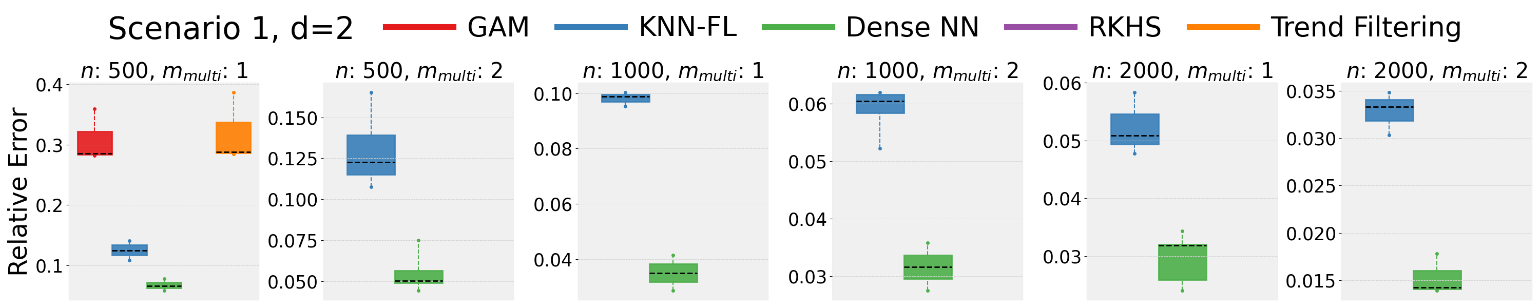
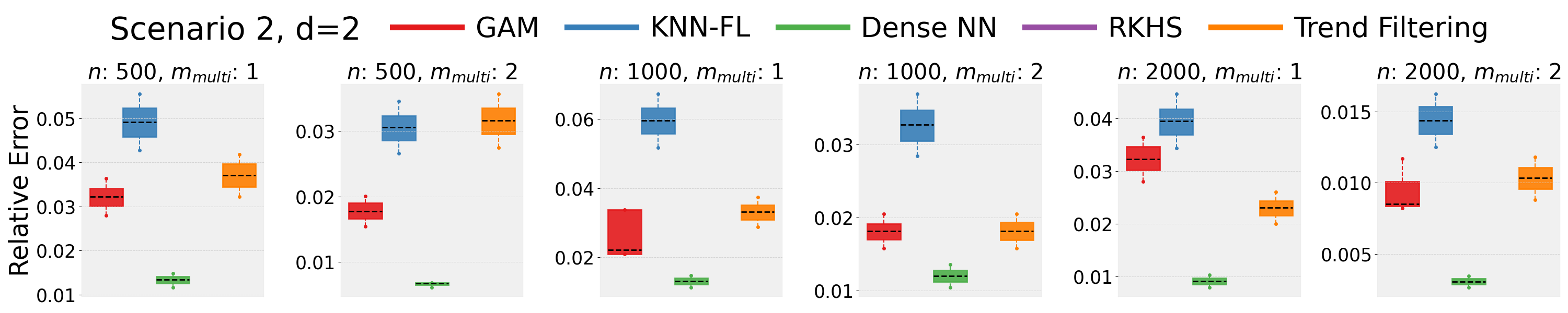
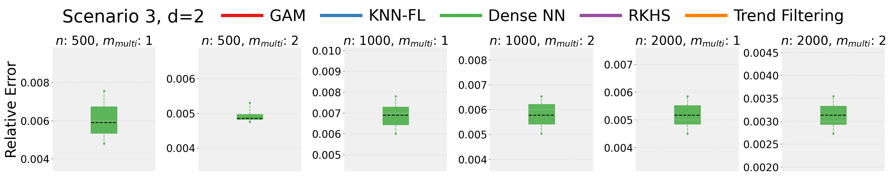
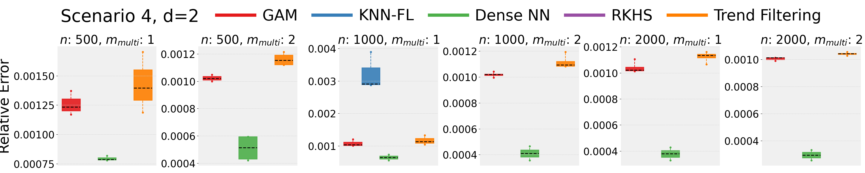
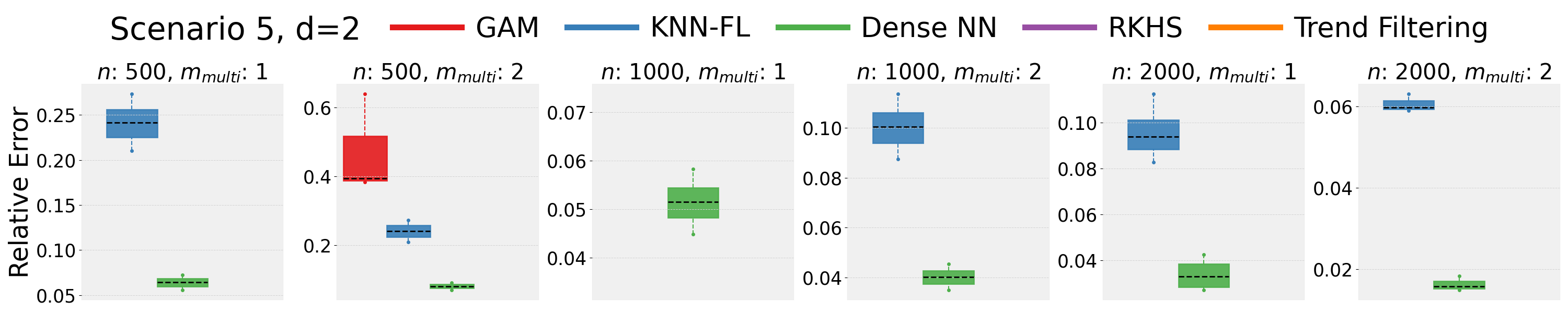
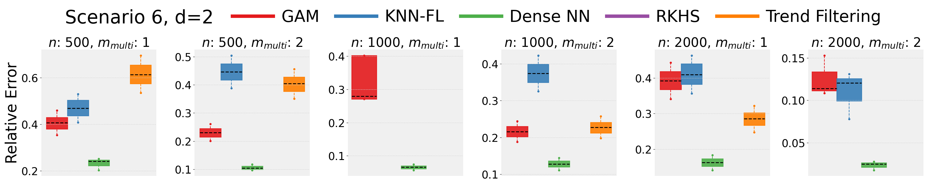
Figure 8: Comparison of methods across different scenarios, $d=2$, $n$, and $m_{mult}$ by box-plot. For each $(n,m_{mult})$ setting, we present the errors of the competitors in the range of within 5 times the smallest error.

In Figure 8 and 9 in the Appendix, we report additional simulations with dimensions $d\in\{2,5\}$. Moreover, also in the Appendix, Tables 5,  6,  7,  8, and  9 give the hyperparameters selected for each competing method.

aboveskip=-1pt, belowskip=-1pt, font=footnotesize

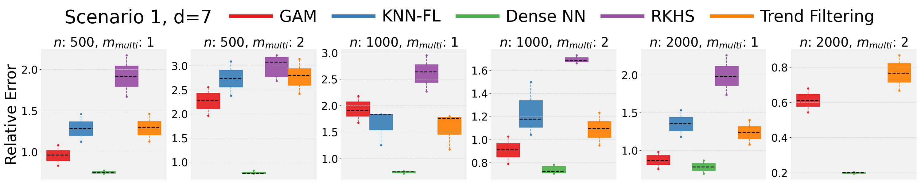
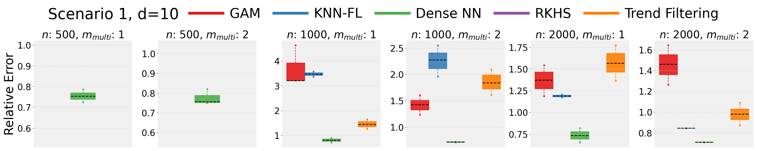
Figure 1: Comparison of methods for Scenario 1 with $d=7$ (top) and $d=10$ (bottom). Each $(n,m_{mult})$ setting presents the errors of the competitors within 5 times the smallest error.

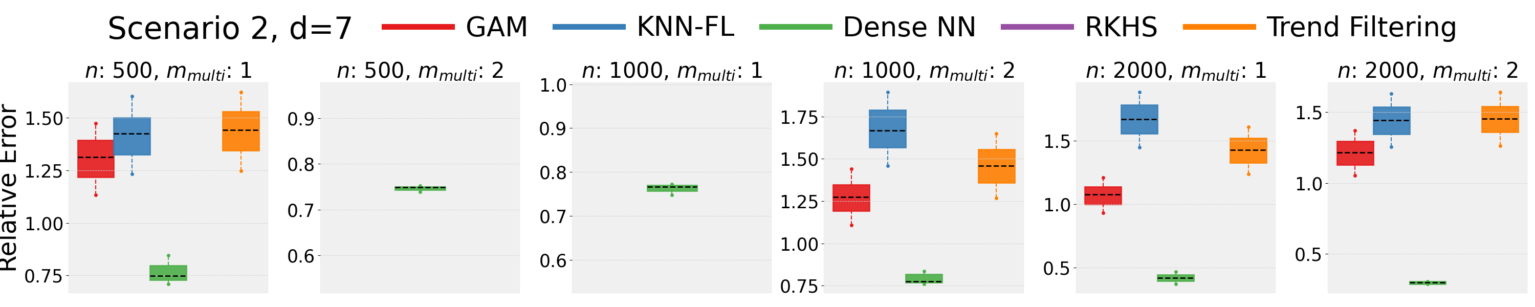
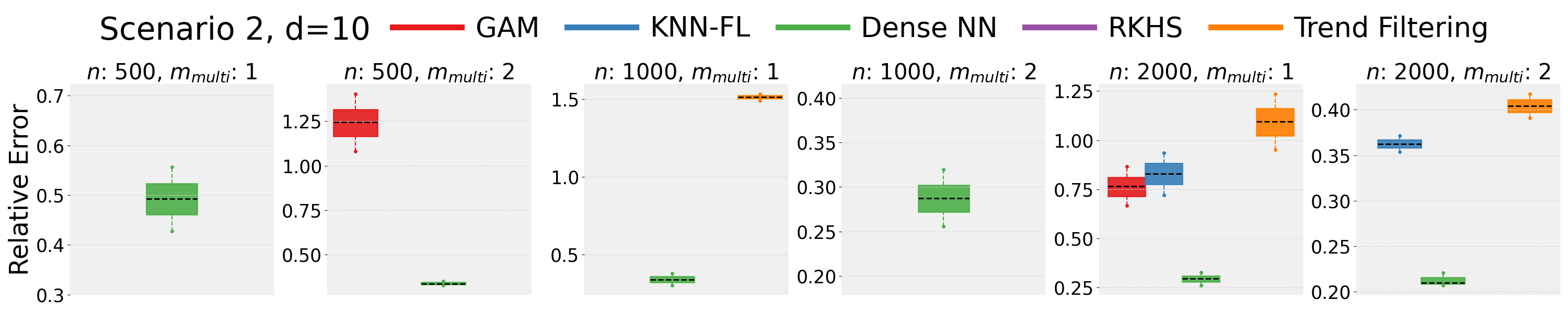
Figure 2: Comparison of methods for Scenario 2.

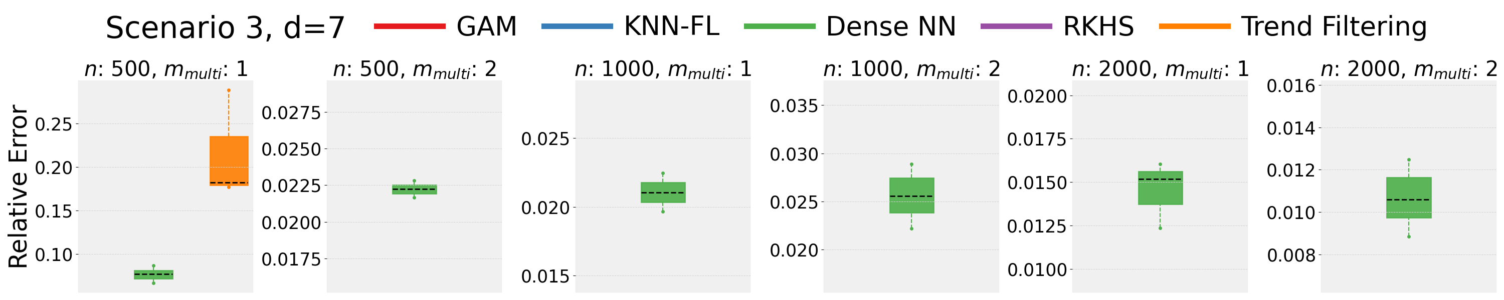
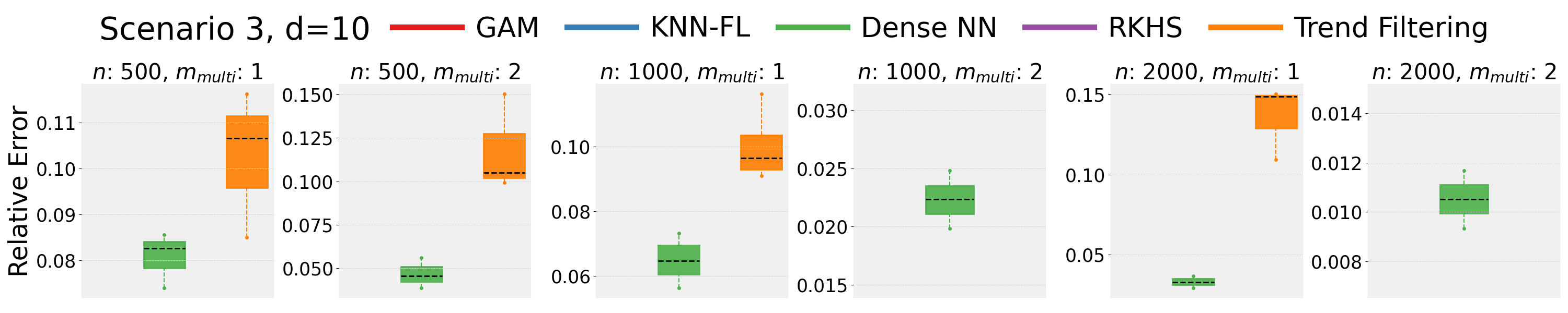
Figure 3: Comparison of methods for Scenario 3.

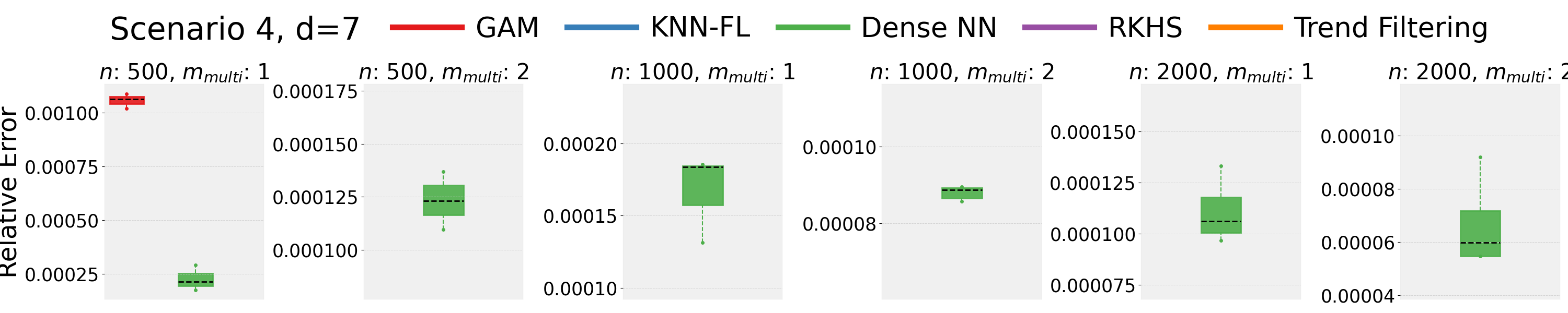
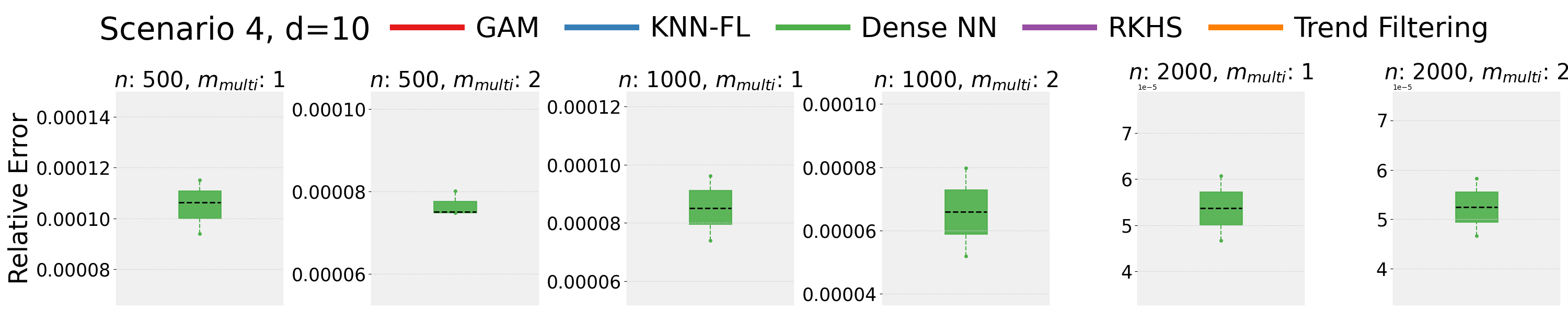
Figure 4: Comparison of methods for Scenario 4.

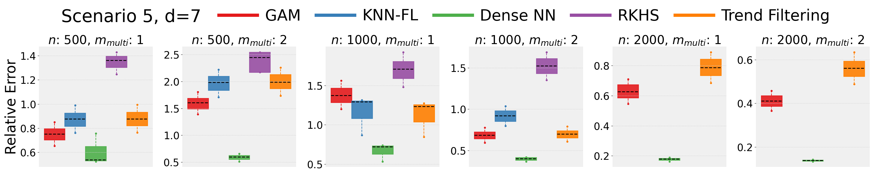
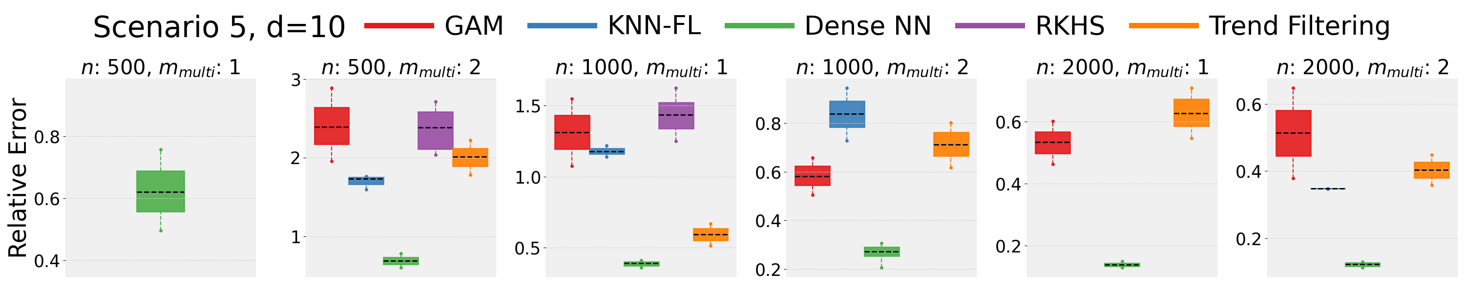
Figure 5: Comparison of methods for Scenario 5.

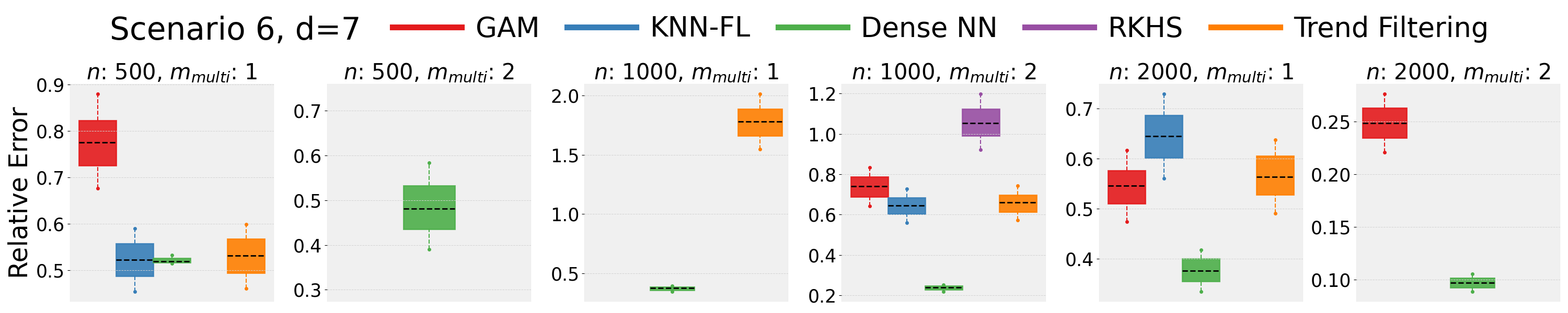
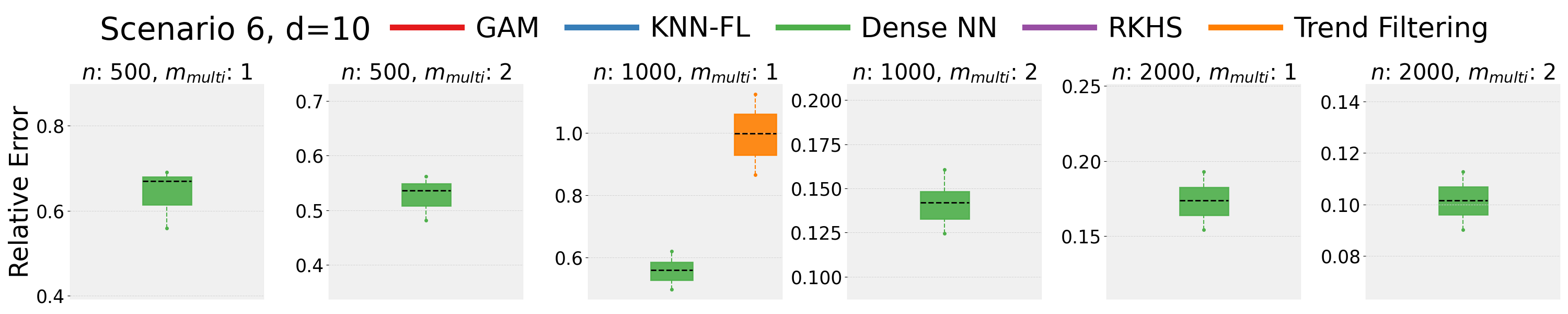
Figure 6: Comparison of methods for Scenario 6.

5.2 Real data application

We consider the EPA Regional dataset, which consists of daily ozone measurements collected across various monitoring stations in different regions of the United States (https://www.epa.gov/enviro/data-downloads). The dataset includes measurements of ozone concentration and associated variables such as Air Quality Index (AQI), wind speed, temperature, Latitude, and Longitude. The specific variables in the dataset are: State Code, County Code, Site Number, Latitude, Longitude, Date (Year, Month, Day), Ozone (in parts per million), AQI, Wind (in miles per hour), and Temperature (in Fahrenheit). Data were collected daily over multiple years.

For our analysis, we focus on predicting daily ozone levels based on these geographic and meteorological variables. We randomly selected monitoring stations across different states in various EPA regions, ensuring a representative variety of locations. The observations cover an entire year of daily measurements. The regions considered include latitude and longitude ranges of $63^{\circ}N-70^{\circ}N$ and $148^{\circ}W-153^{\circ}W$, respectively, including several representative sites across the continental United States.

To implement our analysis, we have applied our proposed Dense NN method alongside other methods such as GAM, KNN-FL, Trend Filtering, and RKHS. For each model, we used daily data from the year 2023. A total of 260 days were considered for each region, with an average of 40 sites per day, resulting in 12,240 measurements. Categorical variables were encoded using one-hot encoding, and numeric variables were scaled to the range $[0,1]$.

We split the data into training and test sets using $75\%/25\%$ splits for each EPA region. All models were trained on the training data, and 5-fold cross-validation was used to select tuning parameters. Prediction performance was evaluated on the test set for each method. We assessed the accuracy of the ozone predictions based on relative error defined as

$$\text{Relative Error}=\frac{\|\hat{f}-y\|_{nm}^{2}}{\|y\|_{nm}^{2}}.$$ (19)

The results provide insights into the effectiveness of different methods for modeling and predicting daily ozone levels based on meteorological variables.

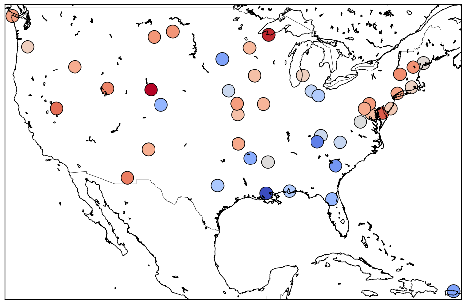
(a) Ozone, $y$

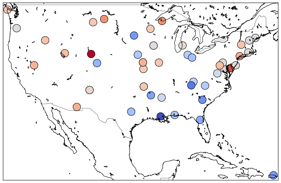
(b) Dense NN, $\hat{y}$

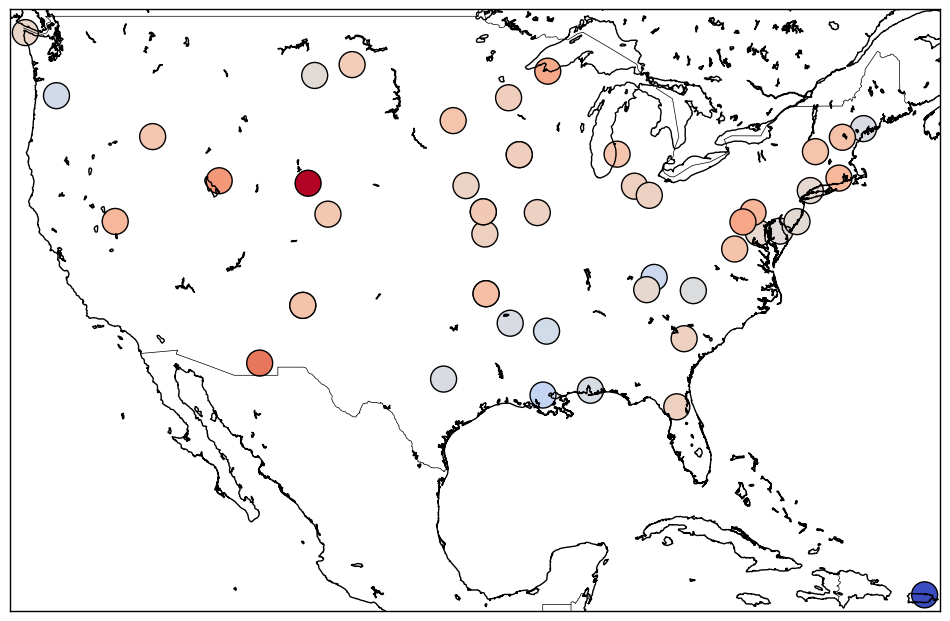
(c) GAM, $\hat{y}$

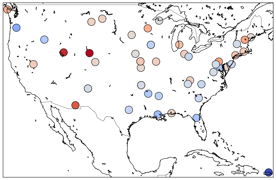
(d) KNN-FL, $\hat{y}$

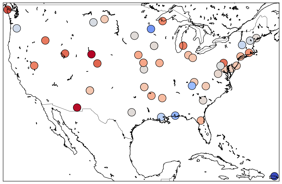
(e) RKHS, $\hat{y}$

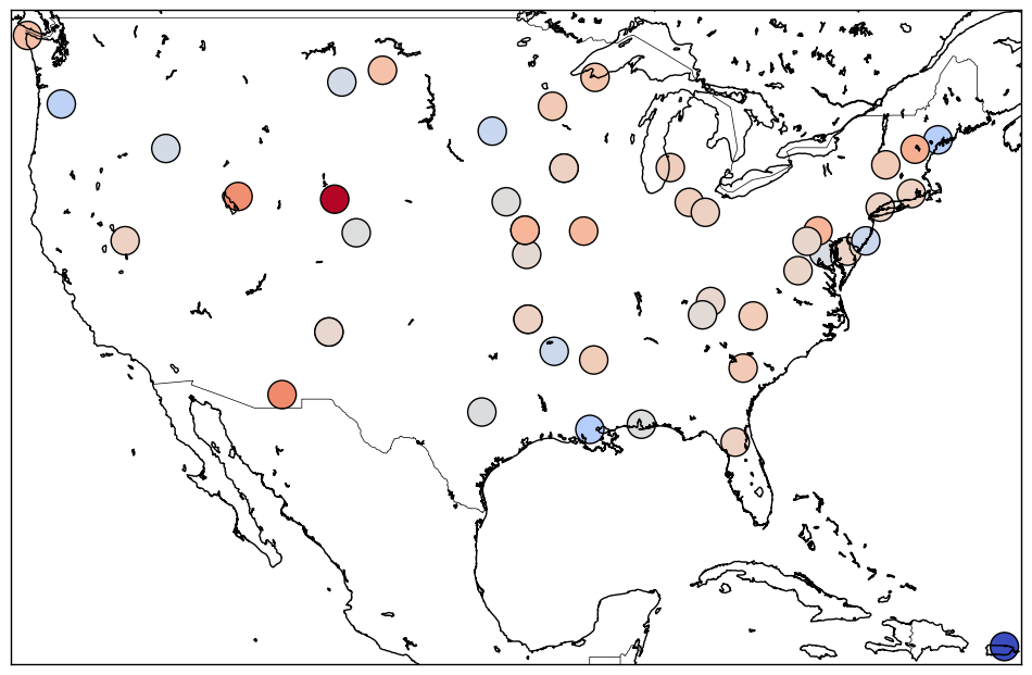
(f) Trend Filtering, $\hat{y}$

Figure 7: Visualization of predicted ozone levels for selected regions on March 3rd. Subplots (a) show the $y$, the observed ozone levels, while subplots (b) to (f) represent predictions from Dense NN, GAM, KNN-FL, RKHS, and Trend Filtering, respectively.

Table 1: Prediction performance (Relative Error) of different methods for ozone level prediction. The values in parentheses represent standard deviations.

Dense NN	GAM	KNN-FL	RKHS	Trend Filtering
0.0086 (0.009)	0.0574 (0.015)	0.0255 (0.010)	0.1374 (0.022)	0.0518 (0.020)

The results, presented in Table 1, show that the Dense NN achieved the lowest relative error among all methods. Figure 7 visualizes the selected regions analyzed in this study. March 3rd was chosen as a representative day from the year-long dataset to streamline the analysis and enhance clarity. The figure’s results further corroborate those presented in Table 1. Our proposed method, Dense NN, produces predictions that are closest to the true ozone levels, as clearly demonstrated in the figures.

6 Outline of the proof of Theorem 3.1, Corollary 3.3 and Corollary 3.4

Theorem 3.1: The proof of Theorem 3.1 is divided into two critical steps. The initial step entails a decomposition of the estimation error, measured via the $\mathcal{L}_{2}$ norm. In doing this, we use two key features. A minimization attribute and the coupling characteristic between empirical and $\mathcal{L}_{2}$ norms. The subsequent step is dedicated to the derivation of deviation bounds. These bounds incorporate Rademacher complexities and pertain to measurement errors as well as spatial noise.

Both stages come with a significant challenge, the interplay between time and space, known as the temporal-spatial dependence. To provide an overview of how we tackled this throughout the proof, in the following we expose our strategy. In Appendix B.2.1, a blocking method is crafted, which effectively transforms dependent $\beta$-mixing sequences into a sequence of independent blocks. The number of these blocks scales as $O(\log(n))$. By analyzing each block independently, we ensure that the examination of the $\beta$-mixing sequences is confined within these blocks. This approach ultimately allows us to analyze a process of length $O(\log(n))$, leveraging the independence within each block to manage the temporal-spatial dependence.
Proof Sketch:

• Step $1$: We find an approximator $\overline{f}\in\mathcal{F}(L,r)$ such that

  $$\left\|f^{*}-\overline{f}\right\|_{\infty}^{2}\leq 2\phi_{nm},$$

  where $\phi_{nm}$ is the upper bound of approximation error for class $\mathcal{F}(L,r)$, as shown in (25). Choosing $\mathcal{A}_{nm}=\max\{\sigma_{\epsilon},\sigma_{\gamma}\}\cdot o\left(\log(nm)\right)$, leads to $\left\|\overline{f}\right\|_{\infty}\leq{\mathcal{A}_{nm}}$.

• Step $2$: Next, we decompose the $\mathcal{L}_{2}$ error of estimator as

  $$\|\widehat{f}_{\mathcal{A}_{nm}}-f^{*}\|_{\mathcal{L}_{2}}^{2}\leq 2\|\overline{f}_{\mathcal{A}_{nm}}-f^{*}\|_{\mathcal{L}_{2}}^{2}+2\|\overline{f}_{\mathcal{A}_{nm}}-\widehat{f}_{\mathcal{A}_{nm}}\|_{\mathcal{L}_{2}}^{2}\leq 4\phi_{nm}+2\|\overline{f}_{\mathcal{A}_{nm}}-\widehat{f}_{\mathcal{A}_{nm}}\|_{\mathcal{L}_{2}}^{2}.$$ (20)

• Step $3$: Our subsequent objective is to transition from the $\mathcal{L}_{2}$ norm to the empirical norm. Lemma B.17 provides a coupling of empirical and $\mathcal{L}_{2}$ norms. Specificially, with high probability,

  $$\left\|\widehat{f}_{\mathcal{A}_{nm}}-\overline{f}_{\mathcal{A}_{nm}}\right\|_{\mathcal{L}_{2}}^{2}\leq 2\left\|\widehat{f}_{\mathcal{A}_{nm}}-\overline{f}_{\mathcal{A}_{nm}}\right\|_{nm}^{2}+C\left\{\phi_{\frac{nm}{S}}\log^{5.3}(\frac{nm}{S})+\mathcal{A}^{2}_{nm}\beta(S)\right\},$$ (21)

  where $S\asymp\log(n)$.

• Step $4$: At this point, coupled with the minimization property of $\widehat{f}_{\mathcal{A}_{nm}}$, it follows that

  $$\frac{1}{2}\left\|\widehat{f}_{\mathcal{A}_{nm}}-\overline{f}_{\mathcal{A}_{nm}}\right\|_{nm}^{2}$$

  $$\leq \frac{1}{32}\|\widehat{f}_{\mathcal{A}_{nm}}-\overline{f}_{\mathcal{A}_{nm}}\|_{nm}^{2}+16\phi_{nm}$$

  $$+ \sum_{i=1}^{n}\sum_{j=1}^{m_{i}}\frac{1}{nm_{i}}\left\{\widehat{f}_{\mathcal{A}_{nm}}(x_{ij})-\overline{f}_{\mathcal{A}_{nm}}(x_{ij})\right\}\left\{\gamma_{i}(x_{ij})+\epsilon_{ij}\right\}.$$

• Step $5$: To analyze the second term where involving $\epsilon_{ij}$, by Lemma G.2 and Corollary B.16, the deviation bounds for $\epsilon$,

  $$\sum_{i=1}^{n}\sum_{j=1}^{m_{i}}\frac{1}{nm_{i}}\left\{\widehat{f}_{\mathcal{A}_{nm}}-\overline{f}_{\mathcal{A}_{nm}}\right\}(x_{ij})\epsilon_{ij}$$

  $$\leq C\mathcal{A}_{nm}\cdot\phi_{\frac{nm}{S}}\left\{\log^{4.3}\left(nm\right)\log(\|\widehat{f}_{\mathcal{A}_{nm}}-\overline{f}_{\mathcal{A}_{nm}}\|_{\frac{nm}{S}}^{-1})\right\}+\frac{1}{32}\left\|\widehat{f}_{\mathcal{A}_{nm}}-\overline{f}_{\mathcal{A}_{nm}}\right\|_{nm}^{2},$$

  with high probability.

  Then by Lemma G.6, Corollary B.10, Lemma B.17, also with high probability, we have

  $$\sum_{i=1}^{n}\sum_{j=1}^{m_{i}}\frac{1}{nm_{i}}\left\{\widehat{f}_{\mathcal{A}_{nm}}-\overline{f}_{\mathcal{A}_{nm}}\right\}(x_{ij})\gamma_{i}(x_{ij})$$

  $$\leq \frac{8\sigma_{\gamma}^{2}}{n}+\frac{3}{16}\left\|\widehat{f}_{\mathcal{A}_{nm}}-\overline{f}_{\mathcal{A}_{nm}}\right\|_{nm}^{2}+C\left\{\mathcal{A}^{2}_{nm}\phi_{\frac{nm}{S}}\log^{5.3}(nm)+\mathcal{A}^{2}_{nm}\beta(S)\right\}.$$

  Putting the previous steps together, it follows that

  $$\left\|\widehat{f}_{\mathcal{A}_{n}}-\overline{f}_{\mathcal{A}_{nm}}\right\|_{nm}^{2}\leq C_{4}\left\{\mathcal{A}_{nm}^{2}\phi_{\frac{nm}{S}}\log^{5.3}(nm)+\mathcal{A}_{nm}^{2}\beta(S)+\frac{1}{n}\right\},$$ (22)

  which, together with (20) and (21), holds with high probability.

  Then, assuming Assumption 3.1 a, choosing $\mathcal{A}_{nm}=\max\{\sigma_{\epsilon},\sigma_{\gamma}\}\cdot o\left(\log(nm)\right)$, and recalling $\phi_{\frac{nm}{S}}=\max_{(p,K)\in\mathcal{P}}\left(\frac{nm}{S}\right)^{-\frac{2p}{2p+K}},$ we obtain the final bound in (3).

Corollary 3.3: The proof of Corollary 3.3 follows similar logic, with t different steps relating the $\mathcal{L}_{2}$ with the empirical norm. Thus, by Lemma B.17, we can show that

$$\left\|\widehat{f}_{\mathcal{A}_{nm}}-\overline{f}_{\mathcal{A}_{nm}}\right\|_{\mathcal{L}_{2}}^{2}\leq 2\left\|\widehat{f}_{\mathcal{A}_{nm}}-\overline{f}_{\mathcal{A}_{nm}}\right\|_{nm}^{2}+C\mathcal{A}_{nm}\phi_{nm}\log^{5.3}(nm).$$ (23)

The rest proofs follow a similar logic where the additional $\beta$ terms appearing in the previous proofs are all gone.

Corollary 3.4: The proof of Corollary 3.4 adheres to a similar trajectory, with the incorporation of simpler step into the first phase of Theorem 3.1. The condition $m_{i}=1$ for all $i$, means that $\left\{x_{ij}\right\}_{i=1,j=1}^{n,m_{i}}$ and $\left\{\epsilon_{ij}\right\}_{i=1,j=1}^{n,m_{i}}$ can replaced by $\left\{x_{i}\right\}_{i=1}^{n}$, noises $\left\{\epsilon_{i}\right\}_{i=1}^{n}$, respectively. This yields

$$\left\|\widehat{f}_{\mathcal{A}_{n}}-f^{*}\right\|_{\mathcal{L}_{2}}^{2}\lesssim(\mathcal{A}_{n}^{2}+1)\phi_{\frac{n}{S}}\log^{5.3}(n)+\mathcal{A}_{n}^{2}\beta(S),$$

where $S\asymp\log(n)$.

7 Outline of the proof of Theorems 4.1

For inputs on a low-dimensional manifold, the approximation theory leads to a different result.

When the input variable $x_{ij}$ is supported on some $d^{*}$-dimensional Lipschitz-manifold $\mathcal{M}\subseteq[0,1]^{d}$, and $d^{*}\in\{1,\ldots,d\}$, the approximation error is $\sqrt{\phi_{nm,\mathcal{M}}}$, presented in (61).

We use $\phi_{nm,\mathcal{M}}$ throughout our proof to derive new deviation bounds.

The proof steps for the manifold case follow a similar logical structure to those in the non-manifold case, thus we omit them.

8 Conclusion and Future Directions

In this paper, we explored the use of fully connected deep neural networks (Dense NN) with ReLU activation functions for nonparametric regression in the presence of both temporal and spatial dependencies in the data. Our study revealed that, even under the complexities of such dependencies, Dense NN can achieve robust non-asymptotic convergence rates. We demonstrated that by incorporating temporal and spatial dependencies, models can better capture the intricate relationships inherent in real-world data, leading to improved predictive performance and theoretical robustness. Furthermore, we addressed the curse of dimensionality by exploring the use of manifold learning, showing that Dense NN can effectively leverage the intrinsic low-dimensional structure of high-dimensional data to achieve better convergence rates.

We extended existing theories in neural network-based nonparametric regression, particularly by incorporating spatial noise and dependence, and provided a detailed analysis of the convergence rates under these more general settings. Our work broadens the scope of neural network applications in nonparametric statistics, offering new insights into the adaptability of Dense NN in complex data environments.

8.1 Future Directions

While this work provides significant advancements in understanding the performance of Dense NN in temporal-spatial data contexts, several avenues for future research remain open:

1. Extension to Higher-Order Function Spaces: Our current framework primarily deals with $(p,C)$-smooth function classes with hierarchical composition structure. Extending the analysis to higher-order smoothness function spaces, especially under temporal-spatial dependence, remains an open challenge. This could involve developing new approximation techniques and error bounds for Dense NN in such spaces.

2. Relaxation of Decay Assumptions: The mixing coefficients in our study are assumed to exhibit exponential decay. Investigating the implications of relaxing this assumption to polynomial decay or other forms of weaker dependencies could provide a broader understanding of the applicability of our results across various temporal-spatial settings.

3. Generalization to Other Activation Functions: Although ReLU is a popular choice due to its computational advantages, exploring the performance of Dense NN with other activation functions under temporal-spatial dependence could lead to more versatile models. Extending our theoretical results to a broader class of activation functions would be a valuable addition.

4. Incorporating Additional Data Structures: Future research could explore incorporating other forms of data structures, such as hierarchical data or network data, into the temporal-spatial framework. This would involve adapting our current models to account for these additional complexities, potentially leading to new insights and applications.

By pursuing these directions, we can continue to refine and expand the theoretical and practical capabilities of Dense NN in nonparametric regression, particularly in complex and high-dimensional data environments.

Appendices

Appendix A Proof of Theorem 3.1

A.1 Preliminary Result for Proof of Theorem 3.1

Lemma A.1 (Neural Networks Approximation Result.).

Let $L_{nm},r_{nm}\in\mathbf{N}$, there exists a neural network $f\in\mathcal{F}(L,r)$ such that it can either take the form as

Case 1. a wide network with $$L=L_{nm}\asymp\log(nm)\quad\text{and}\quad r=r_{nm}\asymp\max_{(p,K)\in\mathcal{P}}(nm)^{\frac{K}{2(2p+K)}},$$

Case 2. a deep network with $$L=L_{nm}\asymp\log(nm)\cdot\max_{(p,K)\in\mathcal{P}}(nm)^{\frac{K}{2(2p+K)}}\quad\text{and}\quad r=O(1).$$ (24)

In either case, it holds that

$$\inf_{f\in\mathcal{F}(L,r)}\|f-f^{*}\|_{\infty}\leq\sqrt{\phi_{nm}},$$ (25)

where

$$\phi_{nm}=\max_{(p,K)\in\mathcal{P}}\left(\sum_{i=1}^{n}m_{i}\right)^{\frac{-2p}{(2p+K)}}\asymp\max_{(p,K)\in\mathcal{P}}\left(nm\right)^{\frac{-2p}{\left(2p+K\right)}},$$

provided $m_{i}\asymp m$ for all $i$.

Proof.

The result follows from Theorem 2 of Kohler and Langer (2019). Theorem 2 of Kohler and Langer (2019) states that: let $d\in\mathbf{N}$, let $f:\mathbb{R}^{d}\rightarrow\mathbb{R}$ be $(p,C)$-smooth for some $p\geq 0$ and $C>0$. Let $M\in\mathbf{N}$ sufficiently large (independent of the size but up to multiplied by a large constant). For $\mathcal{F}(L,r)$, let $L_{nm},r_{nm}\in\mathbf{N}$ such that when $M$ is sufficiently large

$$\text{Case 1}: \text{(i)}\quad\left.L\geq 5+\left\lceil\log_{4}\left(M^{2p}\right)\right\rceil\cdot\left(\left\lceil\log_{2}(\max\{q,d\}+1\}\right)\right\rceil+1\right)$$

$$\text{(ii)}\quad r\geq 2^{d}\cdot 64\cdot\left(\begin{array}[]{c}d+q\\ d\end{array}\right)\cdot d^{2}\cdot(q+1)\cdot M^{d}$$

$$\text{or Case 2}: \text{(i)}\quad L\geq 5M^{d}+\left\lceil\log_{4}\left(M^{2p+4\cdot d\cdot(q+1)}\cdot e^{4\cdot(q+1)\cdot\left(M^{d}-1\right)}\right)\right\rceil\cdot\left\lceil\log_{2}(\max\{q,d\}+1)\right\rceil$$

$$\quad\quad+\left\lceil\log_{4}\left(M^{2\bar{p}}\right)\right\rceil$$

$$\text{(ii)}\quad r\geq 132\cdot 2^{d}\cdot\left\lceil e^{d}\right\rceil\cdot\left(\begin{array}[]{c}d+q\\ d\end{array}\right)\cdot\max\left\{q+1,d^{2}\right\}$$

hold. There exists a neural network $\hat{f}_{\text{net}}\in\mathcal{F}(L,r)$ with the property that

$$\left\|f-\hat{f}_{\text{net}}\right\|_{\infty,[-a,a]^{d}}\lesssim M^{-2p}$$

First, choose $a=1$ and evenly extend the function $f$ above from $\left[0,1\right]^{d}$ to $\left[-1,1\right]^{d}$. Then by choosing $M\asymp\max_{(p,K)\in\mathcal{P}}\left(nm\right)^{\frac{1}{2(2p+K)}}$ in Case 1 above, it suffices to choose $L=L_{nm}\asymp\log\left(\sum_{i=1}^{n}m_{i}\right)\asymp\log\left(nm\right)$ and $r=r_{nm}\asymp\max_{(p,K)\in\mathcal{P}}\left(\sum_{i=1}^{n}m_{i}\right)^{\frac{K}{2(2p+K)}}\asymp\max_{(p,K)\in\mathcal{P}}\left(nm\right)^{\frac{K}{2\left(2p+K\right)}}$. On the other hand, by choosing $M\asymp\max_{(p,K)\in\mathcal{P}}(nm)^{\frac{1}{2(2p+K)}}$in Case 2 above, it suffices to choose $L=L_{nm}\asymp\log(nm)\max_{(p,K)\in\mathcal{P}}\left(nm\right)^{\frac{K}{2(2p+K)}}$ and $r=r_{nm}\asymp 1$.

∎

Overall, we have

$$Lr\asymp\log\left(nm\right)\max_{(p,K)\in\mathcal{P}}\left(nm\right)^{\frac{K}{2(2p+K)}},$$ (26)

$$Lr^{2}\lesssim\log\left(nm\right)\left[\max_{(p,K)\in\mathcal{P}}\left(nm\right)^{\frac{K}{2(2p+K)}}\right]^{2}\lesssim nm.$$

Remark A.1.

The rate above indicates that the networks of the class $\mathcal{F}(L,r)$, which is the so-called fully connected feedfoward neural networks class, can achieve the $\ell_{\infty}$-error bound that does not depend on the dimension of predictors $d$ and therefore circumvents the curse of dimensionality.

Lemma A.2.

Suppose Assumption 3.1 holds, there exists a parameter $\mathcal{B}_{nm}$ depending only on $n$, $m$ and a parameter $\mathcal{C}_{n}$ depending only on $n$, such that

$$\mathbb{P}\left(|\epsilon_{ij}|\leq\sigma_{\epsilon}\cdot\frac{\mathcal{B}_{nm}}{4}\text{ for all }1\leq i\leq n,1\leq j\leq m_{i}\right)=1-o(1),$$ (27)

$$\mathbb{P}\left(\|\gamma_{i}\|_{\infty}\leq\sigma_{\gamma}\cdot\frac{\mathcal{C}_{n}}{4}\text{ for all }1\leq i\leq n\right)=1-o(1),$$ (28)

where $\operatorname*{{\mathbb{E}}}(\epsilon^{2})\leq\sigma_{\epsilon}^{2}<\infty,\sigma_{\gamma}^{2}=\sup_{x\in\left[0,1\right]^{d}}\operatorname*{{\mathbb{E}}}\gamma_{i}(x)^{2}<\infty$.

Proof.

By assuming that $\{\epsilon_{ij}\}_{i=1,j=1}^{n,m_{i}}$ are sub-Gaussian random variables with sub-Gaussian parameter $\sigma_{\epsilon}$, we have

$$\mathbb{P}\left(|\epsilon_{ij}|\leq\sigma_{\epsilon}\cdot\frac{\mathcal{B}_{nm}}{4}\text{ for all }1\leq i\leq n,1\leq j\leq m_{i}\right)$$

$$= 1-\mathbb{P}\left(\max_{i=1,j=1}^{n,m_{i}}|\epsilon_{ij}|\geq\sigma_{\epsilon}\cdot\frac{1}{4}\mathcal{B}_{nm}\right)\geq 1-\left(\sum_{i=1}^{n}m_{i}\right)\exp\left(\sigma_{\epsilon}^{2}\cdot\frac{-\mathcal{B}_{nm}^{2}}{32\sigma_{\epsilon}^{2}}\right)$$

$$\geq 1-\exp\left(\sigma_{\epsilon}^{2}\cdot\frac{-\mathcal{B}_{nm}^{2}}{32\sigma_{\epsilon}^{2}}+\log\left(\sum_{i=1}^{n}{m_{i}}\right)\right).$$

Therefore, it suffices to choose $\mathcal{B}_{nm}\asymp\sqrt{\log(nm)}$. Then it remains to find $\mathcal{C}_{n}$ that satisfies

$$\mathbb{P}(\left\|\gamma_{i}\right\|_{\infty}\leq\sigma_{\gamma}\cdot\frac{\mathcal{C}_{n}}{4}\text{ for all }1\leq i\leq n)$$

$$=1-\mathbb{P}(\max_{1\leq i\leq n}\|\gamma_{i}\|_{\infty}>\sigma_{\gamma}\cdot\frac{\mathcal{C}_{n}}{4})$$

$$\geq 1-n\mathbb{P}(\sup_{x\in[0,1]^{d}}|\gamma_{i}(x)|>\sigma_{\gamma}\cdot\frac{\mathcal{C}_{n}}{4})$$

$$=1-o(1).$$

For each $i=1,2,\ldots,n$, let $\gamma_{i}$ be a separable centered Gaussian process on $[0,1]^{d}$, which is a totally bounded set. If $\sigma_{\gamma}^{2}:=\sup_{x\in\left[0,1\right]^{d}}\mathbb{E}\gamma_{i}(x)^{2}<\infty$, then by Borell’s inequality (see Theorem 5.8 of Boucheron et al. (2013) or Corollary 8.6 of Kühn and Schilling (2023)), for any $u>0$

$$\mathbb{P}\left\{\left|\sup_{x\in\left[0,1\right]^{d}}\gamma_{i}(x)-\mathbb{E}\left[\sup_{x\in\left[0,1\right]^{d}}\gamma_{i}(x)\right]\right|\geq u\right\}\leq 2\exp\left\{-\frac{u^{2}}{2\sigma_{\gamma}^{2}}\right\}.$$

Besides, by Fernique’s theorem (see Corollary 8.7 of Kühn and Schilling (2023)),

$$\mathbb{E}\left[e^{c\left[\sup_{x\in\left[0,1\right]^{d}}\gamma_{i}(x)\right]^{2}}\right]<\infty,\quad 0\leq c<\frac{1}{2}\sigma_{\gamma}.$$

Then there exists $C>0$ such that

$$\mathbb{P}\left\{\sup_{x\in\left[0,1\right]^{d}}\gamma_{i}(x)\geq\frac{1}{2}(C+u)\right\}\leq 2\exp\left\{-\frac{u^{2}}{8\sigma_{\gamma}^{2}}\right\}.$$ (29)

Note that

$$\mathbb{P}\left\{\sup_{x\in\left[0,1\right]^{d}}|{\gamma_{i}(x)}|\geq C+u\right\}$$

$$=\mathbb{P}\left\{\sup_{x\in\left[0,1\right]^{d}}\left[\gamma_{i}^{+}(x)+\gamma_{i}^{-}(x)\right]\geq C+u\right\}$$

$$\leq\mathbb{P}\left\{\sup_{x\in\left[0,1\right]^{d}}\gamma_{i}^{+}(x)+\sup_{x\in\left[0,1\right]^{d}}\gamma_{i}^{-}(x)\geq C+u\right\}$$

$$\leq\mathbb{P}\left\{\sup_{x\in\left[0,1\right]^{d}}\gamma_{i}^{+}(x)\geq\frac{1}{2}(C+u)\right\}+\mathbb{P}\left\{\sup_{x\in\left[0,1\right]^{d}}\gamma_{i}^{-}(x)\geq\frac{1}{2}(C+u)\right\}$$

$$\leq\mathbb{P}\left\{\sup_{x\in\left[0,1\right]^{d}}\gamma_{i}(x)\geq\frac{1}{2}(C+u)\right\}+\mathbb{P}\left\{\sup_{x\in\left[0,1\right]^{d}}-\gamma_{i}(x)\geq\frac{1}{2}(C+u)\right\}$$

$$\leq 4\exp\left\{-\frac{u^{2}}{8\sigma_{\gamma}^{2}}\right\},$$

where given a function $\gamma(x)$, $\gamma^{+}(x)=\max(\gamma(x),0),\gamma^{-}(x)=\max(-\gamma(x),0),$ where the first inequality follows by subadditivity of the supremum, $0<C=2\mathbb{E}\left[\sup_{x\in\left[0,1\right]^{d}}\gamma_{i}(x)\right]<\infty$, and the last inequality holds because $\gamma_{i}$ is symmetric on zero and by (29). Therefore, we have

$$\mathbb{P}\left(\left\|\gamma_{i}\right\|_{\infty}\leq\sigma_{\gamma}\cdot\frac{\mathcal{C}_{n}}{4}\text{ for all }1\leq i\leq n\right)$$

$$\geq 1-n\mathbb{P}\left(\sup_{x\in[0,1]^{d}}\left|\gamma_{i}(x)\right|>\sigma_{\gamma}\cdot\frac{\mathcal{C}_{n}}{4}\right)$$

$$\geq 1-4\exp\left\{-\sigma_{\gamma}^{2}\cdot\frac{(\mathcal{C}_{n}-C)^{2}}{128\sigma_{\gamma}^{2}}+\log(n)\right\}.$$

Combining the arguments above on the tail bounds for $\epsilon$ and $\gamma_{i}$, it suffices to choose $\mathcal{B}_{nm}\asymp\sqrt{\log\left(nm\right)}$, $\mathcal{C}_{n}\asymp\sqrt{\log(n)}$ such that

$$\mathbb{P}\left(\left|\epsilon_{ij}\right|\leq\sigma_{\epsilon}\cdot\frac{\mathcal{B}_{nm}}{4}\text{ for all }1\leq i\leq n,1\leq j\leq m_{i}\right)=1-o(1),$$

and

$$\mathbb{P}\left(\ \left\|\gamma_{i}\right\|_{\infty}\leq\sigma_{\gamma}\cdot\frac{\mathcal{C}_{n}}{4}\text{ for all }1\leq i\leq n\right)=1-o(1).$$

∎

A.2 Proof of Theorem 3.1

To facilitate reading, we provide the Theorem 3.1 again.

Theorem (Theorem 3.1).

Suppose Assumption 3.1 holds and let $\widehat{f}$ be the estimator in $\mathcal{F}(L,r)$ defined in (2), with its number of layers $L$ and number of neurons per layer $r$ set as either one of the two cases:

Case 1. a wide network with $$L\asymp\log(nm)\quad\text{and}\quad r\asymp\max_{(p,K)\in\mathcal{P}}(nm)^{\frac{K}{2(2p+K)}},$$

Case 2. a deep network with $$L\asymp\log(nm)\cdot\max_{(p,K)\in\mathcal{P}}(nm)^{\frac{K}{2(2p+K)}}\quad\text{and}\quad r=O(1).$$ (30)

Let $\mathcal{A}_{nm}\asymp\max\left\{\sigma_{\epsilon},\sigma_{\gamma}\right\}\cdot\log^{1/2}(nm).$ Then with probability approaching to one, it holds that

$$\|\widehat{f}_{\mathcal{A}_{nm}}-f^{*}\|_{\mathcal{L}_{2}}^{2}\lesssim(\mathcal{A}^{2}_{nm}+1)\phi_{\frac{nm}{\log(n)}}\log^{5.3}(nm)+\frac{\mathcal{A}^{2}_{nm}}{n}.$$ (31)

Proof.

Let $\mathcal{A}_{nm}\asymp\max\left\{\sigma_{\epsilon}\cdot\mathcal{B}_{nm},\sigma_{\gamma}\cdot\mathcal{C}_{n}\right\}\asymp\max\left\{\sigma_{\epsilon}\cdot\sqrt{\log(nm)},\sigma_{\gamma}\cdot\sqrt{\log(n)}\right\}$,
or $\max\{\sigma_{\epsilon},\sigma_{\gamma}\}\cdot\sqrt{\log(nm)}$.

Then, we will show that with probability approaching to one, it holds that

$$\|\widehat{f}_{\mathcal{A}_{nm}}-f^{*}\|_{\mathcal{L}_{2}}^{2}\lesssim{\mathcal{A}^{2}_{nm}}\phi_{\frac{nm}{S}}\log^{5.3}(nm)+\mathcal{A}^{2}_{nm}\beta(S)+\frac{\sigma_{\gamma}^{2}}{n},$$

for sufficiently large $n$, with $S\asymp\log(n)$. Finally, by Assumption 3.1 for $\beta$ coefficients, we obtain the bound.

Let $\overline{f}\in\mathcal{F}(L,r)$ be such that

$$\|f^{*}-\overline{f}\|_{\infty}^{2}\leq 2\phi_{nm},$$ (32)

where the existence of $\overline{f}$ is valid by Lemma A.1. Since $\mathcal{A}_{nm}$ can be chosen appropriately large with respect to $n$ while $\phi_{nm}$ decays with respect to $n$, assume that $\sqrt{2\phi_{nm}}\leq\frac{3}{4}\mathcal{A}_{nm}$. In addition, assume $1\leq\mathcal{A}_{nm}=\max\{\sigma_{\epsilon},\sigma_{\gamma}\}\cdot\sqrt{\log(nm)}$ where $m$ and $m_{i}$ satisfy $cm\leq m_{i}\leq Cm$ for any $i=1,2,\ldots,n$. Then,

$$\left\|\overline{f}\right\|_{\infty}\leq\left\|f^{*}\right\|_{\infty}+\left\|f^{*}-\overline{f}\right\|_{\infty}\leq\frac{1}{4}\mathcal{A}_{nm}+\sqrt{2\phi_{nm}}\leq{\mathcal{A}_{nm}},$$

where the second inequality holds by Assumption 3.1 g and (32). It follows that $\overline{f}=\overline{f}_{\mathcal{A}_{nm}}$. Since

$$\|\widehat{f}_{\mathcal{A}_{nm}}-f^{*}\|_{\mathcal{L}_{2}}^{2}\leq 2\|\overline{f}_{\mathcal{A}_{nm}}-f^{*}\|_{\mathcal{L}_{2}}^{2}+2\|\overline{f}_{\mathcal{A}_{nm}}-\widehat{f}_{\mathcal{A}_{nm}}\|_{\mathcal{L}_{2}}^{2}\leq 4\phi_{nm}+2\|\overline{f}_{\mathcal{A}_{nm}}-\widehat{f}_{\mathcal{A}_{nm}}\|_{\mathcal{L}_{2}}^{2},$$

where the second inequality holds by (32), it suffices to show with probability approaching to one,

$$\|\overline{f}_{\mathcal{A}_{nm}}-\widehat{f}_{\mathcal{A}_{nm}}\|_{\mathcal{L}_{2}}^{2}\lesssim{\mathcal{A}^{2}_{nm}}\phi_{\frac{nm}{S}}\log^{5.3}(nm)+\mathcal{A}^{2}_{nm}\beta(S)+\frac{\sigma_{\gamma}^{2}}{n}.$$ (33)

The following steps are made conditioning on $\{x_{ij}\}^{n,m_{i}}_{i=1,j=1}$ except for (36).  
Step 1. Denote the event

$$\mathcal{E}=\left\{|\epsilon_{ij}|\leq\frac{1}{4}\mathcal{A}_{nm}\text{ for all }1\leq i\leq n,1\leq j\leq m_{i}\quad\text{and}\quad\left\|\gamma_{i}\right\|_{\infty}\leq\frac{1}{4}\mathcal{A}_{nm}\text{ for all }1\leq i\leq n\right\}.$$

Suppose the event $\mathcal{E}$ holds. By Lemma A.2, we have

$$\mathbb{P}\left(\left|\epsilon_{ij}\right|\leq\frac{\mathcal{A}_{nm}}{4}\text{ for all }1\leq i\leq n,1\leq j\leq m_{i}\ \text{and}\ \left\|\gamma_{i}\right\|_{\infty}\leq\frac{\mathcal{A}_{nm}}{4}\text{ for all }1\leq i\leq n\right)=1-o(1),$$

or

$$\mathbb{P}\left(\mathcal{E}^{c}\right)=o(1).$$

Note that under $\mathcal{E}$, $|y_{ij}|\leq\|f^{*}\|_{\infty}+|\epsilon_{ij}|+\|\gamma_{i}\|_{\infty}\leq{\mathcal{A}_{nm}}$ for any $1\leq i\leq n,1\leq j\leq m_{i}$. It follows that

$$\sum_{i=1}^{n}\sum_{j=1}^{m_{i}}\frac{1}{nm_{i}}\left(y_{ij}-\widehat{f}_{\mathcal{A}_{nm}}(x_{ij})\right)^{2}\leq\sum_{i=1}^{n}\sum_{j=1}^{m_{i}}\frac{1}{nm_{i}}\left(y_{ij}-\widehat{f}(x_{ij})\right)^{2}.$$ (34)

Additionally, from the minimization property of $\widehat{f}(\cdot)$,

$$\sum_{i=1}^{n}\sum_{j=1}^{m_{i}}\frac{1}{nm_{i}}\left(y_{ij}-\widehat{f}(x_{ij})\right)^{2}\leq\sum_{i=1}^{n}\sum_{j=1}^{m_{i}}\frac{1}{nm_{i}}\left(y_{ij}-\overline{f}(x_{ij})\right)^{2}=\sum_{i=1}^{n}\sum_{j=1}^{m_{i}}\frac{1}{nm_{i}}\left(y_{ij}-\overline{f}_{\mathcal{A}_{nm}}(x_{ij})\right)^{2}$$

where the second identity follows from the fact $\overline{f}=\overline{f}_{\mathcal{A}_{nm}}$ mentioned above. Therefore

$$\sum_{i=1}^{n}\sum_{j=1}^{m_{i}}\frac{1}{nm_{i}}\left(y_{ij}-\widehat{f}_{\mathcal{A}_{nm}}(x_{ij})\right)^{2}\leq\sum_{i=1}^{n}\sum_{j=1}^{m_{i}}\frac{1}{nm_{i}}\left(y_{ij}-\overline{f}_{\mathcal{A}_{nm}}(x_{ij})\right)^{2}.$$ (35)

Rewriting the left-hand side and expanding the squared term, we get

$$\sum_{i=1}^{n}\sum_{j=1}^{m_{i}}\frac{1}{nm_{i}}\left(y_{ij}-\widehat{f}_{\mathcal{A}_{nm}}(x_{ij})\right)^{2} =\sum_{i=1}^{n}\sum_{j=1}^{m_{i}}\frac{1}{nm_{i}}\left[\left(y_{ij}-\overline{f}_{\mathcal{A}_{nm}}(x_{ij})\right)+\left(\overline{f}_{\mathcal{A}_{nm}}(x_{ij})-\widehat{f}_{\mathcal{A}_{nm}}(x_{ij})\right)\right]^{2}$$

$$=\sum_{i=1}^{n}\sum_{j=1}^{m_{i}}\frac{1}{nm_{i}}\left(y_{ij}-\overline{f}_{\mathcal{A}_{nm}}(x_{ij})\right)^{2}$$

$$\quad+\sum_{i=1}^{n}\sum_{j=1}^{m_{i}}\frac{2}{nm_{i}}\left(y_{ij}-\overline{f}_{\mathcal{A}_{nm}}(x_{ij})\right)\left(\overline{f}_{\mathcal{A}_{nm}}(x_{ij})-\widehat{f}_{\mathcal{A}_{nm}}(x_{ij})\right)$$

$$\quad+\sum_{i=1}^{n}\sum_{j=1}^{m_{i}}\frac{1}{nm_{i}}\left(\overline{f}_{\mathcal{A}_{nm}}(x_{ij})-\widehat{f}_{\mathcal{A}_{nm}}(x_{ij})\right)^{2}$$

$$\leq\sum_{i=1}^{n}\sum_{j=1}^{m_{i}}\frac{1}{nm_{i}}\left(y_{ij}-\overline{f}_{\mathcal{A}_{nm}}(x_{ij})\right)^{2}.$$

Subtracting $\sum_{i=1}^{n}\sum_{j=1}^{m_{i}}\frac{1}{nm_{i}}\left(y_{ij}-\overline{f}_{\mathcal{A}_{nm}}(x_{ij})\right)^{2}$ from both sides, we get

$$\sum_{i=1}^{n}\sum_{j=1}^{m_{i}}\frac{1}{nm_{i}}\left(\overline{f}_{\mathcal{A}_{nm}}(x_{ij})-\widehat{f}_{\mathcal{A}_{nm}}(x_{ij})\right)^{2}\leq-\frac{2}{nm}\sum_{i=1}^{n}\sum_{j=1}^{m_{i}}\left(y_{ij}-\overline{f}_{\mathcal{A}_{nm}}(x_{ij})\right)\left(\overline{f}_{\mathcal{A}_{nm}}(x_{ij})-\widehat{f}_{\mathcal{A}_{nm}}(x_{ij})\right),$$

which implies

$$\frac{1}{2}\left\|\widehat{f}_{\mathcal{A}_{nm}}-\overline{f}_{\mathcal{A}_{nm}}\right\|_{nm}^{2}\leq\sum_{i=1}^{n}\sum_{j=1}^{m_{i}}\frac{1}{nm_{i}}\left\{\widehat{f}_{\mathcal{A}_{nm}}(x_{ij})-\overline{f}_{\mathcal{A}_{nm}}(x_{ij})\right\}\left\{y_{ij}-\overline{f}_{\mathcal{A}_{nm}}(x_{ij})\right\}.$$

It follows that

$$\frac{1}{2}\left\|\widehat{f}_{\mathcal{A}_{nm}}-\overline{f}_{\mathcal{A}_{nm}}\right\|_{nm}^{2}$$

$$\leq \sum_{i=1}^{n}\sum_{j=1}^{m_{i}}\frac{1}{nm_{i}}\left\{\widehat{f}_{\mathcal{A}_{nm}}(x_{ij})-\overline{f}_{\mathcal{A}_{nm}}(x_{ij})\right\}\left\{f^{*}(x_{ij})+\gamma_{i}(x_{ij})+\epsilon_{ij}-\overline{f}_{\mathcal{A}_{nm}}(x_{ij})\right\}$$

$$= \sum_{i=1}^{n}\sum_{j=1}^{m_{i}}\frac{1}{nm_{i}}\left\{\widehat{f}_{\mathcal{A}_{nm}}(x_{ij})-\overline{f}_{\mathcal{A}_{nm}}(x_{ij})\right\}\left\{f^{*}(x_{ij})-\overline{f}_{\mathcal{A}_{nm}}(x_{ij})\right\}$$

$$+ \sum_{i=1}^{n}\sum_{j=1}^{m_{i}}\frac{1}{nm_{i}}\left\{\widehat{f}_{\mathcal{A}_{nm}}(x_{ij})-\overline{f}_{\mathcal{A}_{nm}}(x_{ij})\right\}\left\{\gamma_{i}(x_{ij})+\epsilon_{ij}\right\}.$$

Step 2. Note that

$$\sum_{i=1}^{n}\sum_{j=1}^{m_{i}}\frac{1}{nm_{i}}\left\{\widehat{f}_{\mathcal{A}_{nm}}(x_{ij})-\overline{f}_{\mathcal{A}_{nm}}(x_{ij})\right\}\left\{f^{*}(x_{ij})-\overline{f}_{\mathcal{A}_{nm}}(x_{ij})\right\}$$

$$= \sum_{i=1}^{n}\sum_{j=1}^{m_{i}}\frac{1}{nm_{i}}\left\{\widehat{f}_{\mathcal{A}_{nm}}(x_{ij})-\overline{f}_{\mathcal{A}_{nm}}(x_{ij})\right\}\left\{f^{*}(x_{ij})-\overline{f}(x_{ij})\right\}$$

$$\leq \left\|\widehat{f}_{\mathcal{A}_{nm}}-\overline{f}_{\mathcal{A}_{nm}}\right\|_{nm}\sqrt{2\phi_{nm}}$$

$$\leq \frac{1}{32}\|\widehat{f}_{\mathcal{A}_{nm}}-\overline{f}_{\mathcal{A}_{nm}}\|_{nm}^{2}+16\phi_{nm},$$

where the first inequality follows from the definition of empirical norm $\left\|\cdot\right\|_{nm}$ and (32).

Step 3. By Lemma G.2 and Corollary B.16,

$$\sum_{i=1}^{n}\sum_{j=1}^{m_{i}}\frac{1}{nm_{i}}\left\{\widehat{f}_{\mathcal{A}_{nm}}-\overline{f}_{\mathcal{A}_{nm}}\right\}(x_{ij})\epsilon_{ij}$$

$$\leq C_{1}^{\prime\prime}\sigma_{\epsilon}^{2}\cdot\phi_{\frac{nm}{S}}\left\{\log^{4.3}\left(nm\right)\log(\mathcal{A}_{nm}\cdot\|\widehat{f}_{\mathcal{A}_{nm}}-\overline{f}_{\mathcal{A}_{nm}}\|_{\frac{nm}{S}}^{-1})\right\}+\frac{1}{32}\left\|\widehat{f}_{\mathcal{A}_{nm}}-\overline{f}_{\mathcal{A}_{nm}}\right\|_{nm}^{2}$$

$$\leq C_{1}^{\prime\prime\prime}\mathcal{A}_{nm}\cdot\phi_{\frac{nm}{S}}\left\{\log^{4.3}\left(nm\right)\log(\|\widehat{f}_{\mathcal{A}_{nm}}-\overline{f}_{\mathcal{A}_{nm}}\|_{\frac{nm}{S}}^{-1})\right\}+\frac{1}{32}\left\|\widehat{f}_{\mathcal{A}_{nm}}-\overline{f}_{\mathcal{A}_{nm}}\right\|_{nm}^{2},$$

where the last inequality follows from the assumption that ${\mathcal{A}_{nm}}=o(\log(nm))$ when $nm$ is sufficiently large.  
Step 4. By Lemma B.17,

$$\left\|\widehat{f}_{\mathcal{A}_{nm}}-\overline{f}_{\mathcal{A}_{nm}}\right\|_{\mathcal{L}_{2}}^{2}\leq 2\left\|\widehat{f}_{\mathcal{A}_{nm}}-\overline{f}_{\mathcal{A}_{nm}}\right\|_{nm}^{2}+C\left\{\phi_{\frac{nm}{S}}\log^{5.3}(\frac{nm}{S})+\mathcal{A}^{2}_{nm}\beta(S)\right\},$$ (36)

Observe that

$$\sum_{i=1}^{n}\sum_{j=1}^{m_{i}}\frac{1}{nm_{i}}\left[\widehat{f}_{\mathcal{A}_{nm}}-\overline{f}_{\mathcal{A}_{nm}}\right](x_{ij})\gamma_{i}(x_{ij})$$

$$= \sum_{i=1}^{n}\sum_{j=1}^{m_{i}}\frac{1}{nm_{i}}\left\{\left[\widehat{f}_{\mathcal{A}_{nm}}-\overline{f}_{\mathcal{A}_{nm}}\right](x_{ij})\gamma_{i}(x_{ij})-\langle\gamma_{i},\widehat{f}_{\mathcal{A}_{nm}}-\overline{f}_{\mathcal{A}_{nm}}\rangle_{\mathcal{L}_{2}}\right\}+\frac{1}{n}\sum_{i=1}^{n}\langle\gamma_{i},\widehat{f}_{\mathcal{A}_{nm}}-\overline{f}_{\mathcal{A}_{nm}}\rangle_{\mathcal{L}_{2}}$$

and that

$$\frac{1}{n}\sum_{i=1}^{n}\left\langle\gamma_{i},\widehat{f}_{\mathcal{A}_{nm}}-\overline{f}_{\mathcal{A}_{nm}}\right\rangle_{\mathcal{L}_{2}}=\left\langle\frac{1}{n}\sum_{i=1}^{n}\gamma_{i},\widehat{f}_{\mathcal{A}_{nm}}-\overline{f}_{\mathcal{A}_{nm}}\right\rangle_{\mathcal{L}_{2}}\leq\left\|\frac{1}{n}\sum_{i=1}^{n}\gamma_{i}\right\|_{\mathcal{L}_{2}}\left\|\widehat{f}_{\mathcal{A}_{nm}}-\overline{f}_{\mathcal{A}_{nm}}\right\|_{\mathcal{L}_{2}}$$

$$\leq \frac{\sigma_{\gamma}^{2}}{\sqrt{n}}\left\|\widehat{f}_{\mathcal{A}_{nm}}-\overline{f}_{\mathcal{A}_{nm}}\right\|_{\mathcal{L}_{2}}\leq\frac{8\sigma_{\gamma}^{2}}{n}+\frac{1}{32}\left\|\widehat{f}_{\mathcal{A}_{nm}}-\overline{f}_{\mathcal{A}_{nm}}\right\|_{\mathcal{L}_{2}}^{2}$$

$$\leq \frac{8\sigma_{\gamma}^{2}}{n}+\frac{1}{16}\left\|\widehat{f}_{\mathcal{A}_{nm}}-\overline{f}_{\mathcal{A}_{nm}}\right\|_{nm}^{2}+C\left\{\phi_{\frac{nm}{S}}\log^{5.3}(\frac{nm}{S})+\mathcal{A}^{2}_{nm}\beta(S)\right\},$$

where the second inequality follows from Lemma G.6 and the last inequality follows from Lemma B.17.

In addition,

$$\sum_{i=1}^{n}\sum_{j=1}^{m_{i}}\frac{1}{nm_{i}}\left\{\big{[}\widehat{f}_{\mathcal{A}_{nm}}-\overline{f}_{\mathcal{A}_{nm}}\big{]}(x_{ij})\gamma_{i}(x_{ij})-\langle\gamma_{i},\widehat{f}_{\mathcal{A}_{nm}}-\overline{f}_{\mathcal{A}_{nm}}\rangle_{\mathcal{L}_{2}}\right\}$$

$$\leq \frac{1}{16}\|\widehat{f}_{\mathcal{A}_{nm}}-\overline{f}_{\mathcal{A}_{nm}}\|_{\mathcal{L}_{2}}^{2}+C\sigma_{\gamma}\mathcal{C}_{n}\phi_{nm}\log^{5.3}(nm)$$

$$\leq \frac{1}{8}\|\widehat{f}_{\mathcal{A}_{nm}}-\overline{f}_{\mathcal{A}_{nm}}\|_{nm}^{2}+C^{\prime\prime}\left\{\phi_{\frac{nm}{S}}\log^{5.3}(\frac{nm}{S})+\mathcal{A}^{2}_{nm}\beta(S)\right\}+C\sigma_{\gamma}\mathcal{C}_{n}\phi_{nm}\log^{5.3}(nm)$$

where the first inequality follows from Corollary B.10 , and the second inequality follows from Lemma B.17.

Step 5. Putting the previous steps together, it follows that

$$\frac{1}{2}\|\widehat{f}_{\mathcal{A}_{nm}}-\overline{f}_{\mathcal{A}_{nm}}\|_{nm}^{2}$$

$$\leq \frac{1}{32}\|\widehat{f}_{\mathcal{A}_{nm}}-\overline{f}_{\mathcal{A}_{nm}}\|_{nm}^{2}+16\phi_{nm}$$

$$+ C_{1}^{\prime\prime}\sigma_{\epsilon}^{2}\cdot\phi_{\frac{nm}{S}}\left\{\log^{4.3}(nm)\log(\left\|\widehat{f}_{\mathcal{A}_{nm}}-\overline{f}_{\mathcal{A}_{nm}}\right\|_{\frac{nm}{S}}^{-1})\right\}+\frac{1}{32}\left\|\widehat{f}_{\mathcal{A}_{nm}}-\overline{f}_{\mathcal{A}_{nm}}\right\|_{nm}^{2}$$

$$+ \frac{8\sigma_{\gamma}^{2}}{n}+\frac{1}{16}\left\|\widehat{f}_{\mathcal{A}_{nm}}-\overline{f}_{\mathcal{A}_{nm}}\right\|_{nm}^{2}+C\sigma_{\gamma}\mathcal{C}_{n}\phi_{nm}\log^{5.3}(nm)$$

$$+ \frac{1}{8}\|\widehat{f}_{\mathcal{A}_{nm}}-\overline{f}_{\mathcal{A}_{nm}}\|_{nm}^{2}+C^{\prime\prime}\left\{\phi_{\frac{nm}{S}}\log^{5.3}(\frac{nm}{S})+\mathcal{A}^{2}_{nm}\beta(S)\right\}$$

$$\leq \frac{1}{4}\left\|\widehat{f}_{\mathcal{A}_{nm}}-\overline{f}_{\mathcal{A}_{nm}}\right\|_{nm}^{2}+$$

$$C_{1}\left\{\sigma_{\epsilon}^{2}\phi_{\frac{nm}{S}}\log^{4.3}(nm)\log(\left\|\widehat{f}_{\mathcal{A}_{nm}}-\overline{f}_{\mathcal{A}_{nm}}\right\|_{\frac{nm}{S}}^{-1})+\phi_{\frac{nm}{S}}\log^{5.3}(nm)+\mathcal{A}^{2}_{nm}\beta(S)+\frac{\sigma_{\gamma}^{2}}{n}\right\},$$

or simply

$$\|\widehat{f}_{\mathcal{A}_{nm}}-\overline{f}_{\mathcal{A}_{nm}}\|_{nm}^{2}$$ (37)

$$\leq C_{2}\left\{\mathcal{A}^{2}_{nm}\phi_{\frac{nm}{S}}\log^{4.3}(nm)\log(\|\widehat{f}_{\mathcal{A}_{nm}}-\overline{f}_{\mathcal{A}_{nm}}\|_{\frac{nm}{S}}^{-1})+\phi_{\frac{nm}{S}}\log^{5.3}(nm)+\mathcal{A}^{2}_{nm}\beta(S)+\frac{\mathcal{A}^{2}_{nm}}{n}\right\}.$$ (38)

If $\|\widehat{f}_{\mathcal{A}_{nm}}-\overline{f}_{\mathcal{A}_{nm}}\|^{2}_{\frac{nm}{S}}\leq\frac{1}{n}$, then (37) holds. Otherwise, if $\|\widehat{f}_{\mathcal{A}_{nm}}-\overline{f}_{\mathcal{A}_{nm}}\|^{2}_{\frac{nm}{S}}\geq\frac{1}{n}$, then (37) implies

$$\|\widehat{f}_{\mathcal{A}_{nm}}-\overline{f}_{\mathcal{A}_{nm}}\|_{nm}^{2}\leq C_{3}\left\{\phi_{\frac{nm}{S}}\log^{5.3}(nm)+\mathcal{A}^{2}_{nm}\phi_{\frac{nm}{S}}\log^{4.3}(nm)\log(n)+\mathcal{A}^{2}_{nm}\beta(S)+\frac{\mathcal{A}^{2}_{nm}}{n}\right\}$$

$$\leq 2C_{3}\left\{\mathcal{A}^{2}_{nm}\phi_{\frac{nm}{S}}\log^{5.3}(nm)+\mathcal{A}^{2}_{nm}\beta(S)+\frac{\mathcal{A}^{2}_{nm}}{n}\right\}.$$

Thus (37) gives

$$\left\|\widehat{f}_{\mathcal{A}_{n}}-\overline{f}_{{\mathcal{A}_{nm}}}\right\|_{nm}^{2}\leq(2C_{3}+1)\left\{\mathcal{A}^{2}_{nm}\phi_{\frac{nm}{S}}\log^{5.3}(nm)+\mathcal{A}^{2}_{nm}\beta(S)+\frac{\mathcal{A}^{2}_{nm}}{n}\right\},$$ (39)

which together with (36), which holds with high probability with respect to the probability on $\{x_{ij}\}^{n,m_{i}}_{i=1,j=1}$.

So the above implies that, up to a constant, the rate is

$$(\mathcal{A}^{2}_{nm}+1)\left(\frac{S}{nm}\right)^{\frac{2p}{2p+K}}\log^{5.3}(nm)+\mathcal{A}_{nm}^{2}\beta(S)+\frac{\sigma_{\gamma}^{2}}{n}.$$

Our rate is for the truncated estimator $\widehat{f}_{\mathcal{A}_{nm}}$.

a. By choosing $\mathcal{A}_{nm}\asymp\max\left\{\sigma_{\epsilon},\sigma_{\gamma}\right\}\cdot\sqrt{\log(nm)}$ based on Lemma A.2;

b. By Assumption 3.1, if the mixing rate $\beta(S)\lesssim\exp(-C_{\beta}S)$, then it suffices to choose $S=O(\log(n))$.

a and b imply the rate is

$$\left(\sigma_{\epsilon}^{2}+\sigma_{\gamma}^{2}+1\right)\left(\frac{1}{nm}\right)^{\frac{2p}{2p+K}}\log^{7.3}(nm)+\frac{\left(\sigma_{\epsilon}^{2}+\sigma_{\gamma}^{2}\right)\log(nm)}{n}+\frac{\sigma_{\gamma}^{2}}{n}.$$

which gives the rate in (31). The rate holds by selecting the network architecture in (30) to guarantee the approximation error.

∎

Corollary A.3 (Polynomial Decay for Mixing Coefficient).

Under the setting in Theorem 3.1, If $\beta(S)\lesssim S^{-\alpha}$ for some $\alpha>0$. We can achieve the rate

$$\frac{\sigma_{\epsilon}^{2}+\sigma_{\gamma}^{2}+1}{n^{\alpha}}\log^{6.3}(nm)+\frac{\sigma_{\gamma}^{2}}{n},$$

with $S=n$ and $m\geq n^{\alpha(\frac{2p+K}{2p})}.$ If $m\leq n^{\alpha(\frac{2p+K}{2p})},$ we achieve the rate

$$(nm)^{\frac{-2p}{2p+K}}\log^{6.3}(nm)+\frac{\sigma_{\gamma}^{2}}{n},$$

with $S=(nm)^{\frac{2p}{2p+2p\alpha+\alpha K}}$ and $\alpha\to\infty$.

Proof.

Case a. If $\beta(S)\lesssim S^{-\alpha}$ for some $\alpha>0$, and

$$m\leq n^{\alpha(\frac{2p+K}{2p})}.$$

Then $S=(nm)^{\frac{2p}{2p+2p\alpha+\alpha K}}\leq n$ is a valid choice of $S$ and this implies the error bound is

$$\left(\sigma_{\epsilon}^{2}+\sigma_{\gamma}^{2}+1\right)(nm)^{\frac{-2p\alpha}{2p+2p\alpha+\alpha K}}\log^{6.3}(nm)+\left(\sigma_{\epsilon}^{2}+\sigma_{\gamma}^{2}\right)(nm)^{\frac{-2p\alpha}{2p+2p\alpha+\alpha K}}\log(nm)+\frac{\sigma_{\gamma}^{2}}{n}.$$

When $\alpha\to\infty$, so that the data are independent, it follows that this rate goes to

$$(nm)^{\frac{-2p}{2p+K}}\log^{6.3}(nm)+\frac{\sigma_{\gamma}^{2}}{n}.$$

Case b. If $\beta(S)\lesssim S^{-\alpha}$ and

$$m\geq n^{\alpha(\frac{2p+K}{2p})}.$$

Then $S=n$ is a valid choice and this implies the error bound is

$$\left(\sigma_{\epsilon}^{2}+\sigma_{\gamma}^{2}+1\right)\cdot m^{\frac{-2p}{2p+K}}\log^{6.3}(nm)+\frac{\sigma_{\epsilon}^{2}+\sigma_{\gamma}^{2}}{n^{\alpha}}\log^{2}(nm)+\frac{\sigma_{\gamma}^{2}}{n}$$

$$\leq\left(\sigma_{\epsilon}^{2}+\sigma_{\gamma}^{2}+1\right)\cdot\left(\frac{1}{n^{\alpha}}\log^{6.3}(nm)+\frac{1}{n^{\alpha}}\log^{2}(nm)\right)+\frac{\sigma_{\gamma}^{2}}{n}\leq\frac{\sigma_{\epsilon}^{2}+\sigma_{\gamma}^{2}+1}{n^{\alpha}}\log^{6.3}(nm)+\frac{\sigma_{\gamma}^{2}}{n}.$$

∎

Appendix B Additional Technical Results for Theorem 3.1

B.1 Deviation Bounds for Independent Case

The proof below assumes the data are independent, meaning the $\beta$ coefficients are all zero. We focus on the independent case here, and address the dependent case later in Section B.2.

Let $g\in\mathcal{L}_{2}$ and recall

$$\left\|g\right\|_{nm}^{2}=\frac{1}{n}\sum_{i=1}^{n}\frac{1}{m_{i}}\sum_{j=1}^{m_{i}}g^{2}\left(x_{ij}\right)=\sum_{i=1}^{n}\sum_{j=1}^{m_{i}}\frac{1}{nm_{i}}g^{2}\left(x_{ij}\right).$$

Let $m$ be the is the harmonic mean of $\left\{m_{i}\right\}_{i=1}^{n}$ defined as

$$m=\left(\frac{1}{n}\sum_{i=1}^{n}\frac{1}{m_{i}}\right)^{-1}.$$

By the assumption that

$$cm\leq m_{i}\leq Cm,$$

it follows that for any $i=1,2,\cdots,n$,

$$\frac{1}{Cm}\leq\frac{1}{m_{i}}\leq\frac{1}{cm}.$$

B.1.1 Deviation bounds for $\epsilon$

In this section, we assume $\epsilon$ is a vector of independent random variables. The general case is given in Section B.2.2. Denote

$$D_{nm}\left(g\right)=\sum_{i=1}^{n}\sum_{j=1}^{m_{i}}\frac{1}{\sqrt{nm_{i}}}g\left(x_{ij}\right)\epsilon_{ij}.$$

In this section, the analysis is made conditioning on $\left\{x_{ij}\right\}_{i=1,j=1}^{n,m_{i}}$. We denote the conditional probability conditioning on $\left\{x_{ij}\right\}_{i=1,j=1}^{n,m_{i}}$ by $\mathbb{P}_{\cdot\mid\left\{x_{ij}\right\}_{i=1,j=1}^{n,m_{i}}}$, and we use $\mathbb{P}_{\cdot\mid x}$ as its shorthand notation.

Corollary B.1.

Let $g,f\in{\mathcal{L}_{2}}$ be two deterministic functions. Then there exists a constant $c>0$ such that

$$\mathbb{P}_{\cdot\mid x}\left(D_{nm}(g)\geq t\right)\leq\exp\left(-\frac{ct^{2}}{\sigma_{\epsilon}^{2}\cdot\left\|g\right\|_{nm}^{2}}\right),$$ (40)

$$\mathbb{P}_{\cdot\mid x}\left(D_{nm}(g)-D_{nm}(f)\geq t\right)\leq\exp\left(-\frac{ct^{2}}{\sigma_{\epsilon}^{2}\cdot\left\|f-g\right\|_{nm}^{2}}\right).$$ (41)

Proof.

Since $\left\{\epsilon_{ij}\right\}_{i=1,j=1}^{n,m_{i}}$ are i.i.d. from a sub-Gaussian distribution with sub-Gaussian parameter $\sigma_{\epsilon}$. Conditioning on $\left\{x_{ij}\right\}_{i=1,j=1}^{n,m_{i}}$, the first bound is a direct consequence of classical Hoeffding bound. To see this, notice that for $\left\{g(x_{ij})\epsilon_{ij}\right\}_{i=1,j=1}^{n,m_{i}}$ are independent sub-Gaussian variables with sub-Gaussian parameter $|g(x_{ij})|\sigma_{\epsilon}$. This implies that $D_{nm}(g)=\sum_{i=1}^{n}\sum_{j=1}^{m_{i}}\frac{1}{\sqrt{nm_{i}}}g\left(x_{ij}\right)\epsilon_{ij}$ is sub-Gaussian with sub-Gaussian parameters

$$\sqrt{\sigma_{\epsilon}^{2}\sum_{i=1}^{n}\sum_{j=1}^{m_{i}}\frac{1}{nm_{i}}g^{2}\left(x_{ij}\right)}=\sigma_{\epsilon}\left\|g\right\|_{nm}.$$

The second bound holds from the linearity of $D_{nm}(g)$ with respect to g: for $i=1,\dots,n$, $j=1,\dots,m_{i}$, conditioning on $x_{ij}$, $\left[g\left(x_{ij}\right)-f\left(x_{ij}\right)\right]\epsilon_{ij}$ are independent sub-Gaussian variables with sub-Gaussian parameter $\left|\left(g-f\right)\left(x_{ij}\right)\right|\sigma_{\epsilon}$. Then conditioning on $\left\{x_{ij}\right\}_{i=1,j=1}^{n,m_{i}}$,

$$D_{nm}(g)-D_{nm}(f)=\sum_{i=1}^{n}\sum_{j=1}^{m_{i}}\frac{1}{\sqrt{nm_{i}}}\left[g\left(x_{ij}\right)-f\left(x_{ij}\right)\right]\epsilon_{ij}$$

is sub-Gaussian with parameter $\sqrt{\sigma_{\epsilon}^{2}\sum_{i=1}^{n}\sum_{j=1}^{m_{i}}\frac{1}{nm_{i}}\left[(g-f)(x_{ij})\right]^{2}}=\sigma_{\epsilon}\left\|g-f\right\|_{nm}$.

By the same arguments for the first and second inequality, it immediately follows that

$$\mathbb{P}_{\cdot\mid x}\left(D_{nm}(g)\geq t\right) \leq\exp\left(-\frac{c_{0}t^{2}}{\sigma_{\epsilon}^{2}\cdot\sum_{i=1}^{n}\sum_{j=1}^{m_{i}}\frac{1}{nm_{i}}g^{2}(x_{ij})}\right)$$

$$\leq\exp\left(-\frac{c_{0}t^{2}}{\sigma_{\epsilon}^{2}\cdot\left\|g\right\|_{nm}^{2}}\right),$$

$$\mathbb{P}_{\cdot\mid x}\left(D_{nm}(g)-D_{nm}(f)\geq t\right) \leq\exp\left(-\frac{c_{0}t^{2}}{\sigma_{\epsilon}^{2}\cdot\sum_{i=1}^{n}\sum_{j=1}^{m_{i}}\frac{1}{nm_{i}}\left[g(x_{ij})-f(x_{ij})\right]^{2}}\right)$$

$$\leq\exp\left(-\frac{c_{0}t^{2}}{\sigma_{\epsilon}^{2}\cdot\left\|f-g\right\|_{nm}^{2}}\right).$$

∎

Next, for $\lambda>0$, we introduce the notation

$$B_{nm}\left(\lambda\right)=\left\{g:\left\|g\right\|_{nm}\leq\lambda\right\}.$$

Corollary B.2.

Let $\mathcal{F}$ be a function class such that

$$\log\mathcal{N}\left(\delta,\mathcal{F},\left\|\cdot\right\|_{nm}\right)\leq C^{\prime}nm\phi_{nm}\left(\log^{4.3}(nm)\log\left(\delta^{-1}\right)\right).$$ (42)

For

$$t\geq\lambda\sqrt{2C^{\prime}\phi_{nm}nm\left\{\log^{4.3}(nm)\log\left(\lambda^{-1}\right)\right\}}$$

with $\lambda\leq\frac{1}{4}$, it holds that

$$\mathbb{P}_{\cdot\mid x}\left(\sup_{g\in\mathcal{F}\cap B_{nm}\left(\lambda\right)}D_{nm}(g)\geq\sigma_{\epsilon}\cdot t\right)\leq\exp\left(-\frac{c^{\prime}t^{2}}{\lambda^{2}}\right),$$

for some positive constants $c^{\prime}$ and $C^{\prime}$.

Proof.

For $l\in\mathbf{Z}^{+}$, let $\mathcal{T}_{l}$ be the $2^{-l}\lambda$ covering set of $\mathcal{F}\cap B_{nm}\left(\lambda\right)$. Then by setting $\delta=2^{-l}\lambda$ in (42),

$$\left|\mathcal{T}_{l}\right|\leq\exp\left(C^{\prime}nm\phi_{nm}\log^{4.3}(nm)\left\{l\log(2)+\log(\lambda^{-1})\right\}\right).$$

Denote $\psi_{l}(g)\in\mathcal{T}_{l}$ be such that

$$\left\|g-\psi_{l}(g)\right\|_{nm}\leq 2^{-l}\lambda.$$

Step 1. Observe that by union bound,

$$\mathbb{P}_{\cdot\mid x}\left(\sup_{g\in\mathcal{F}\cap B_{nm}\left(\lambda\right)}D_{nm}\left(g\right)\geq\sigma_{\epsilon}\cdot t\right)$$ (43)

$$\leq\mathbb{P}_{\cdot\mid x}\left(\sup_{g\in\mathcal{F}\cap B_{nm}\left(\lambda\right)}D_{nm}\left(\psi_{0}\left(g\right)\right)\geq\sigma_{\epsilon}\cdot t/2\right)$$

$$+\mathbb{P}_{\cdot\mid x}\left(\sup_{g\in\mathcal{F}\cap B_{nm}(\lambda)}D_{nm}(g)-D_{nm}(\psi_{0}(g))\geq\sigma_{\epsilon}\cdot t/2\right).$$

Since $D_{nm}(\psi_{0}(g))$ is sub-Gaussian with parameter $\left\|\psi_{0}(g)\right\|_{nm}\sigma_{\epsilon}\leq\lambda\sigma_{\epsilon}$, it follows that

$$\mathbb{P}_{\cdot\mid x}\left(\sup_{g\in\mathcal{F}\cap B_{nm}(\lambda)}D_{nm}(\psi_{0}(g))\geq\sigma_{\epsilon}\cdot t/2\right)$$ (44)

$$\leq \mathbb{P}_{\cdot\mid x}\left(\sup_{\psi_{0}(g)\in\mathcal{T}_{0}}D_{nm}(\psi_{0}(g))\geq\sigma_{\epsilon}\cdot t/2\right)$$

$$\leq \sum_{\psi_{0}(g)\in\mathcal{T}_{0}}\mathbb{P}_{\cdot\mid x}\left(D_{nm}(\psi_{0}(g))\geq\sigma_{\epsilon}\cdot t/2\right)$$

$$\leq \exp\left(C^{\prime}nm\phi_{nm}\left\{\log^{4.3}(nm)\log(\lambda^{-1})\right\}-\frac{c_{0}t^{2}}{\lambda^{2}}\right)$$

$$\leq \exp\left(-\frac{c_{0}t^{2}}{2\lambda^{2}}\right),$$

where the last inequality follows if $t\geq\lambda\sqrt{2C^{\prime}\phi_{nm}nm\left\{\log^{4.3}(nm)\log(\lambda^{-1})\right\}}.$

Step 2. Note that

$$D_{nm}(\psi_{0}(g))-D_{nm}(g)=\sum_{l=1}^{\infty}D_{nm}(\psi_{l-1}(g))-D_{nm}(\psi_{l}(g)).$$

Therefore, for $\eta_{l}\geq 0$ and $\sum_{l=1}^{\infty}\eta_{l}\leq 1$,

$$\mathbb{P}_{\cdot\mid x}\left(\sup_{g\in\mathcal{F}\cap B_{nm}(\lambda)}D_{nm}(g)-D_{nm}(\psi_{0}(g))\geq\sigma_{\epsilon}\cdot t/2\right)$$

$$\leq \mathbb{P}_{\cdot\mid x}\left(\exists l\in Z^{+},\text{such that}\sup_{g\in\mathcal{F}\cap B_{nm}(\lambda)}D_{nm}(\psi_{l}(g))-D_{nm}(\psi_{l-1}(g))\geq\eta_{l}\sigma_{\epsilon}\cdot t/2\right)$$

$$= \mathbb{P}_{\cdot\mid x}\left(\bigcup_{l=1}^{\infty}\left\{\sup_{g\in\mathcal{F}\cap B_{nm}(\lambda)}D_{nm}(\psi_{l}(g))-D_{nm}(\psi_{l-1}(g))\geq\eta_{l}\sigma_{\epsilon}\cdot t/2\right\}\right)$$

$$\leq \sum_{l=1}^{\infty}\mathbb{P}_{\cdot\mid x}\left(\sup_{g\in\mathcal{F}\cap B_{nm}(\lambda)}D_{nm}(\psi_{l}(g))-D_{nm}(\psi_{l-1}(g))\geq\eta_{l}\sigma_{\epsilon}\cdot t/2\right)$$

$$= \sum_{l=1}^{\infty}\mathbb{P}_{\cdot\mid x}\left(\sup_{\psi_{l-1}(g)\in\mathcal{T}_{l-1},\psi_{l}(g)\in\mathcal{T}_{l}}D_{nm}(\psi_{l}(g))-D_{nm}(\psi_{l-1}(g))\geq\eta_{l}\sigma_{\epsilon}\cdot t/2\right)$$

$$\leq \sum_{l=1}^{\infty}\sum_{\psi_{l-1}(g)\in\mathcal{T}_{l-1},\psi_{l}(g)\in\mathcal{T}_{l}}\mathbb{P}_{\cdot\mid x}\left(D_{nm}(\psi_{l-1}(g)-\psi_{l}(g))\geq\eta_{l}\sigma_{\epsilon}\cdot t/2\right).$$

Since

$$\|\psi_{l-1}(g)-\psi_{l}(g)\|_{nm}\leq\|\psi_{l-1}(g)-g\|_{nm}+\|\psi_{l}(g)-g\|_{nm}\leq 2^{-l+1}\lambda+2^{-l}\lambda=3\cdot 2^{-l}\lambda\leq 2^{-l+2}\lambda,$$

and

$$\left|\mathcal{T}_{l-1}\right|\leq\left|\mathcal{T}_{l}\right|\leq\exp\left(C^{\prime}nm\phi_{nm}\log^{4.3}(nm)\left\{l\log(2)+\log\left(\lambda^{-1}\right)\right\}\right),$$

by plugging $\|\psi_{l-1}(g)-\psi_{l}(g)\|_{nm}\leq 2^{-l+2}\lambda$ in (41),

$$\mathbb{P}_{\cdot\mid x}\left(\sup_{g\in\mathcal{F}\cap B_{nm}(\lambda)}D_{nm}(g)-D_{nm}(\psi_{0}(g))\geq\sigma_{\epsilon}\cdot t/2\right)$$

$$\leq \sum_{l=1}^{\infty}\sum_{\psi_{l-1}(g)\in\mathcal{T}_{l-1},\psi_{l}(g)\in\mathcal{T}_{l}}\mathbb{P}_{\cdot\mid x}\left(D_{nm}(\psi_{l-1}(g)-\psi_{l}(g))\geq\eta_{l}\sigma_{\epsilon}\cdot t/2\right)$$

$$\leq \sum_{l=1}^{\infty}2\exp\left(C^{\prime}nm\phi_{nm}\log^{4.3}(nm)\left\{l\log(2)+\log\left(\lambda^{-1}\right)\right\}\right)\exp\left(-\frac{c^{\prime\prime}2^{2l}\eta_{l}^{2}t^{2}}{\lambda^{2}}\right),$$

for some $c^{\prime\prime}>0$. 
If $C^{\prime}nm\phi_{nm}\log^{4.3}(nm)\left\{l\log(2)+\log(\lambda^{-1})\right\}\leq\frac{c^{\prime\prime}2^{2l}\eta_{l}^{2}t^{2}}{2\lambda^{2}}$, or simply

$$\eta_{l}^{2}\geq\frac{2C^{\prime}\lambda^{2}nm\phi_{nm}\log^{4.3}(nm)\left\{l\log(2)+\log(\lambda^{-1})\right\}}{c^{\prime\prime}t^{2}2^{2l}},$$ (45)

following the previous derivation, we have

$$\mathbb{P}_{\cdot\mid x}\left(\sup_{g\in\mathcal{F}\cap B_{nm}(\lambda)}D_{nm}(g)-D_{nm}(\psi_{0}(g))\geq\sigma_{\epsilon}\cdot t/2\right)$$

$$\leq \sum_{l=1}^{\infty}2\exp\left(C^{\prime}nm\phi_{nm}\log^{4.3}(nm)\left\{l\log(2)+\log\left(\lambda^{-1}\right)\right\}\right)\exp\left(-\frac{c^{\prime\prime}2^{2l}\eta_{l}^{2}t^{2}}{\lambda^{2}}\right)$$

$$\leq \sum_{l=1}^{\infty}2\exp\left(-\frac{c^{\prime\prime}2^{2l}\eta_{l}^{2}t^{2}}{2\lambda^{2}}\right).$$

Since $t\geq\lambda\sqrt{2C^{\prime}\phi_{nm}nm\log^{4.3}(nm)\log(\lambda^{-1})}$, we have

$$\frac{2C^{\prime}\lambda^{2}nm\phi_{nm}\log^{4.3}(nm)\left\{l\log(2)+\log(\lambda^{-1})\right\}}{c^{\prime\prime}t^{2}2^{2l}}$$

$$\leq \frac{1}{c^{\prime\prime}2^{2l}}+\frac{l\log(2)}{\log(\lambda^{-1})c^{\prime\prime}2^{2l}}=\frac{l}{c^{\prime\prime}2^{2l}}\left(\frac{1}{l}+\frac{\log(2)}{\log(\lambda^{-1})}\right)$$

$$\leq \frac{C_{1}l}{c^{\prime\prime}2^{2l}},$$

for some constant $\frac{1}{2}>C_{1}>0$, where the last inequality holds by $\lambda\leq\frac{1}{4}$.

Thus, to satisfy (45), it suffices to choose $\eta_{l}^{2}=C_{1}l2^{-2l}$ for some positive constant $C_{1}$. Furthermore, with such $\eta_{l}$, we have $\sum_{l=1}^{\infty}\eta_{l}=\sqrt{C_{1}}\sum_{l=1}^{\infty}l^{1/2}2^{-l}.$ For large $l$, $2^{-l}$ decreases exponentially faster than $l^{1/2}$ increases, so the series $\sum_{l=1}^{\infty}l^{1/2}2^{-l}$ converges. And further by $\frac{1}{2}>C_{1}$, we have $\sum_{l=1}^{\infty}\eta_{l}\leq 1$. Thus

$$\mathbb{P}_{\cdot\mid x}\left(\sup_{g\in\mathcal{F}\cap B_{nm}(\lambda)}D_{nm}(g)-D_{nm}(\psi_{0}(g))\geq\sigma_{\epsilon}\cdot t/2\right)$$ (46)

$$\leq\sum_{l=1}^{\infty}2\exp\left(-\frac{c^{\prime\prime}lt^{2}}{2\lambda^{2}}\right)\leq\exp(-\frac{c^{\prime\prime\prime}t^{2}}{2\lambda^{2}}).$$

for some positive constant $c^{\prime\prime\prime}$. By (43), (44), (46), we have

$$\mathbb{P}_{\cdot\mid x}\left(\sup_{g\in\mathcal{F}\cap B_{nm}\left(\lambda\right)}D_{nm}(g)\geq\sigma_{\epsilon}\cdot t\right)\leq\exp\left(-\frac{c^{\prime}t^{2}}{\lambda^{2}}\right),$$

for some positive constant $c^{\prime}$. ∎

Corollary B.3.

Let $\mathcal{F}$ be a function class such that

$$\log\mathcal{N}(\delta,\mathcal{F},\|\cdot\|_{nm})\leq C^{\prime}nm\phi_{nm}\left(\log^{4.3}(nm)\log(\delta^{-1})\right)$$ (47)

and that $\mathcal{F}\subset B_{\infty}\left(\tau\right)$, where $\tau\leq\frac{1}{2}$. Then it holds that for any $s\geq 1$,

$$\mathbb{P}_{\cdot\mid x}\left(\sup_{g\in\mathcal{F}}\frac{D_{mn}\left(g\right)}{\left\|g\right\|_{nm}\sqrt{nm\phi_{nm}\left\{\log^{4.3}(nm)\log(\|g\|_{nm}^{-1})\right\}}}\geq C_{1}\sigma_{\epsilon}\cdot s\right)$$

$$\leq C_{2}\exp(-cs^{2}nm\phi_{nm}\log^{4.3}(nm)).$$

Proof.

Since $\mathcal{F}\subset B_{\infty}\left(\tau\right)\subset B_{nm}\left(\tau\right)$, it holds that

$$\mathcal{F}\cap B_{nm}\left(\tau\right)=\mathcal{F}.$$

Therefore, it suffices to show that for any $s\geq 1$,

$$\mathbb{P}_{\cdot\mid x}\left(\sup_{g\in\mathcal{F}\cap B_{nm}\left(\tau\right)}\frac{D_{mn}\left(g\right)}{\left\|g\right\|_{nm}\sqrt{nm\phi_{nm}\left\{\log^{4.3}(nm)\log\left(\|g\|_{nm}^{-1}\right)\right\}}}\geq C_{1}\sigma_{\epsilon}\cdot s\right)$$

$$\leq C_{2}\exp(-cs^{2}nm\phi_{nm}\log^{4.3}(nm)).$$

Choose $\lambda=2^{-l+1}\tau$ in Corollary B.2. For a positive constant $C_{1}^{\prime}$ that depends on $C^{\prime}$, if $s\geq 1$ and

$$t\geq C_{1}^{\prime}s2^{-l+1}\tau\sqrt{nm\phi_{nm}\left\{\log^{4.3}(nm)\log\left((2^{-l+1}\tau)^{-1}\right)\right\}},$$

it holds that

$$\mathbb{P}_{\cdot\mid x}\left(\sup_{g\in\mathcal{F}\cap B_{nm}(2^{-l+1}\tau)}D_{nm}(g)\geq C_{1}^{\prime}\sigma_{\epsilon}\cdot s2^{-l+1}\tau\sqrt{nm\phi_{nm}\left\{\log^{4.3}(nm)\log(\tau^{-1}2^{l-1})\right\}}\right)$$

$$\leq \exp\left(-c^{\prime\prime}s^{2}nm\phi_{nm}\left\{\log^{4.3}(nm)\log(\tau^{-1}2^{l-1})\right\}\right)$$

$$\leq \exp\left(-c^{\prime\prime}s^{2}nm\phi_{nm}\log^{4.3}(nm)l\log(2)\right):=\exp\left(-c^{\prime\prime\prime}s^{2}nm\phi_{nm}\log^{4.3}(nm)l\right),$$

for some positive constants $c^{\prime\prime}$ and $c^{\prime\prime\prime}$, where the second inequality holds since $\tau\leq\frac{1}{2}$, so $\tau^{-1}2^{l-1}\geq 2^{l}$. Thus,

$$\mathbb{P}_{\cdot\mid x}\left(\sup_{g\in\mathcal{F}\cap\left\{f:2^{-l}\tau\leq\|f\|_{nm}\leq 2^{-l+1}\tau\right\}}D_{nm}(g)\right.$$

$$\quad\left.\geq C_{1}^{\prime}\sigma_{\epsilon}\cdot s2^{-l+1}\tau\sqrt{nm\phi_{nm}\left(\log^{4.3}(nm)\log(\tau^{-1}2^{l-1})\right)}\right)$$

$$\leq\exp\left(-c^{\prime\prime\prime}s^{2}nm\phi_{nm}\log^{4.3}(nm)l\right).$$

Note that if $g\in\{f:2^{-l}\tau\leq\|f\|_{nm}\leq 2^{-l+1}\tau\}$, then $\|g\|^{-1}_{nm}\geq\tau^{-1}2^{l-1}$ and $2^{-l+1}\tau\leq 2\left\|g\right\|_{nm}$. It follows that

$$\mathbb{P}_{\cdot\mid x}\left(\sup_{g\in\mathcal{F}\cap\{f:2^{-l}\tau\leq\|f\|_{nm}\leq 2^{-l+1}\tau\}}D_{nm}(g)\right.$$

$$\quad\left.\geq C_{1}^{\prime}\sigma_{\epsilon}\cdot s2^{-l+1}\tau\sqrt{nm\phi_{nm}\left\{\log^{4.3}(nm)\log(\tau^{-1}2^{l-1})\right\}}\right)$$

$$= \mathbb{P}_{\cdot\mid x}\left(\sup_{g\in\mathcal{F}\cap\{f:2^{-l}\tau\leq\|f\|_{nm}\leq 2^{-l+1}\tau\}}\frac{D_{mn}\left(g\right)}{2^{-l+1}\tau\sqrt{nm\phi_{nm}\left\{\log^{4.3}(nm)\log(\tau^{-1}2^{l-1})\right\}}}\geq C_{1}^{\prime}\sigma_{\epsilon}\cdot s\right)$$

$$\geq \mathbb{P}_{\cdot\mid x}\left(\sup_{g\in\mathcal{F}\cap\{f:2^{-l}\tau\leq\|f\|_{nm}\leq 2^{-l+1}\tau\}}\frac{D_{mn}\left(g\right)}{2\left\|g\right\|_{nm}\sqrt{nm\phi_{nm}\left\{\log^{4.3}(nm)\log(\|g\|^{-1}_{nm})\right\}}}\geq C_{1}^{\prime}\sigma_{\epsilon}\cdot s\right)$$

$$= \mathbb{P}_{\cdot\mid x}\left(\sup_{g\in\mathcal{F}\cap\{f:2^{-l}\tau\leq\|f\|_{nm}\leq 2^{-l+1}\tau\}}\frac{D_{mn}\left(g\right)}{\left\|g\right\|_{nm}\sqrt{nm\phi_{nm}\left\{\log^{4.3}(nm)\log(\|g\|^{-1}_{nm})\right\}}}\geq 2C_{1}^{\prime}\sigma_{\epsilon}\cdot s\right).$$

Thus,

$$\mathbb{P}_{\cdot\mid x}\left(\sup_{g\in\mathcal{F}\cap\{f:2^{-l}\tau\leq\|f\|_{nm}\leq 2^{-l+1}\tau\}}\frac{D_{mn}\left(g\right)}{\|g\|_{nm}\sqrt{nm\phi_{nm}\left\{\log^{4.3}(nm)\log\left(\|g\|_{nm}^{-1}\right)\right\}}}\geq C_{1}\sigma_{\epsilon}\cdot s\right)$$

$$\leq \exp\left(-c^{\prime\prime\prime\prime}s^{2}nm\phi_{nm}\log^{4.3}(nm)l\right).$$

Therefore,

$$\mathbb{P}_{\cdot\mid x}\left(\sup_{g\in\mathcal{F}\cap B_{nm}\left(\tau\right)}\frac{D_{nm}(g)}{\|g\|_{nm}\sqrt{nm\phi_{nm}\left\{\log^{4.3}(nm)\log(\|g\|_{nm}^{-1})\right\}}}\geq C_{1}\sigma_{\epsilon}\cdot s\right)$$

$$= \ \mathbb{P}_{\cdot\mid x}\Bigg{(}\exists l\in Z^{+},\text{such that}$$

$$\ \sup_{g\in\mathcal{F}\cap\left\{f:2^{-l}\tau\leq\|f\|_{nm}\leq 2^{-l+1}\tau\right\}}\frac{D_{nm}(g)}{\|g\|_{nm}\sqrt{nm\phi_{nm}\left\{\log^{4.3}(nm)\log(\|g\|_{nm}^{-1})\right\}}}\geq C_{1}\sigma_{\epsilon}\cdot s\Bigg{)}$$

$$\leq \sum_{l=1}^{\infty}\mathbb{P}_{\cdot\mid x}\left(\sup_{g\in\mathcal{F}\cap\{f:2^{-l}\tau\leq\|f\|_{nm}\leq 2^{-l+1}\tau\}}\frac{D_{nm}(g)}{\|g\|_{nm}\sqrt{nm\phi_{nm}\left\{\log^{4.3}(nm)\log(\|g\|_{nm}^{-1})\right\}}}\right.$$

$$\quad\left.\geq C_{1}\sigma_{\epsilon}\cdot s\right)$$

$$\leq \sum_{l=1}^{\infty}\exp\left(-c^{\prime\prime\prime\prime}s^{2}nm\phi_{nm}\log^{4.3}(nm)l\right)$$

$$\leq C_{2}\exp(-cs^{2}nm\phi_{nm}\log^{4.3}(nm)),$$

where the first identity follows from a peeling argument, noticing that $\bigcup_{l=1}^{\infty}\mathcal{F}\cap\{f:2^{-l}\tau\leq\|f\|_{nm}\leq 2^{-l+1}\tau\}=\mathcal{F}\cap\bigcup_{l=1}^{\infty}\{f:2^{-l}\tau\leq\|f\|_{nm}\leq 2^{-l+1}\tau\}=\mathcal{F}\cap B_{nm}(\tau)$. ∎

B.1.2 Deviation bounds for $\xi$

Suppose $\{\xi_{ij}\}_{i=1,j=1}^{n,m_{i}}$ are i.i.d. Rademacher random variables and denote

$$H(g)=\sum_{i=1}^{n}\sum_{j=1}^{m_{i}}\frac{1}{\sqrt{nm_{i}}}g^{2}(x_{ij})\xi_{ij}.$$

In Corollary B.4, Corollary B.5 and Corollary B.6, the analysis is conditioning on $\{x_{ij}\}_{i=1,j=1}^{n,m_{i}}$. We denote the conditional probability conditioning on $\left\{x_{ij}\right\}_{i=1,j=1}^{n,m_{i}}$ by $\mathbb{P}_{\cdot\mid x}$.

Corollary B.4.

Let $g,f\in{\mathcal{L}_{2}}$ be two deterministic functions such that $\|g\|_{\infty}\leq\tau,\|f\|_{\infty}\leq\tau$. Then there exists a constant $c>0$ such that

$$\mathbb{P}_{\cdot\mid x}\left(H\left(g\right)\geq t\right)\leq\exp\left(-\frac{ct^{2}}{\tau^{2}\left\|g\right\|_{mn}^{2}}\right),$$

$$\mathbb{P}_{\cdot\mid x}\left(H\left(g\right)-H\left(f\right)\geq t\right)\leq\exp\left(-\frac{ct^{2}}{\tau^{2}\|f-g\|_{mn}^{2}}\right).$$

Proof.

For the first bound, it suffices to note that $\left\{g^{2}(x_{ij})\xi_{ij}\right\}_{i=1,j=1}^{n,m_{i}}$’s are independent sub-Gaussian with parameter $g^{2}(x_{ij})$. So $H(g)$ is sub-Gaussian with parameter

$$\sqrt{\sum_{i=1}^{n}\sum_{j=1}^{m_{i}}\frac{1}{nm_{i}}g^{4}(x_{ij})}\leq\tau\left\|g\right\|_{mn},$$

since $\left\|g\right\|_{\infty}\leq\tau$. For the second bound, it suffices to note that $\left\{\left(f^{2}(x_{ij})-g^{2}(x_{ij})\right)\xi_{ij}\right\}_{i=1,j=1}^{n,m_{i}}$ are independent sub-Gaussian with parameter $\left\{|f^{2}(x_{ij})-g^{2}(x_{ij})|\right\}_{i=1,j=1}^{n,m_{i}}$. So $H(f)-H(g)$ is sub-Gaussian with parameter

$$\sqrt{\sum_{i=1}^{n}\sum_{j=1}^{m_{i}}\frac{1}{nm_{i}}(f^{2}(x_{ij})-g^{2}(x_{ij}))^{2}}=\sqrt{\sum_{i=1}^{n}\sum_{j=1}^{m_{i}}\frac{1}{nm_{i}}(f(x_{ij})-g(x_{ij}))^{2}(f(x_{ij})+g(x_{ij}))^{2}}$$

$$\leq\sqrt{\sum_{i=1}^{n}\sum_{j=1}^{m_{i}}\frac{4\tau^{2}}{nm_{i}}(f(x_{ij})-g(x_{ij}))^{2}}\leq 2\tau\|f-g\|_{mn}.$$

Since $\|g\|_{\infty}\leq\tau,\|f\|_{\infty}\leq\tau$, the claim follows. ∎

Corollary B.5.

Let $\mathcal{F}$ be a function class such that

$$\log\mathcal{N}(\delta,\mathcal{F},\|\cdot\|_{nm})\leq C^{\prime}nm\phi_{nm}\left(\log^{4.3}(nm)\log(\delta^{-1})\right),$$

and suppose that $g\in\mathcal{F}$ implies that $\|g\|_{\infty}\leq\tau$. For

$$t\geq C^{\prime\prime}\lambda\tau\sqrt{nm\phi_{nm}\left\{\log^{4.3}(nm)\log(\lambda^{-1})\right\}}$$

with $\tau\leq\frac{1}{2}$, it holds that

$$\mathbb{P}_{\cdot\mid x}\left(\sup_{g\in\mathcal{F}\cap B_{nm}(\lambda)}H_{nm}(g)\geq t\right)\leq\exp(-\frac{c^{\prime}t^{2}}{\tau^{2}\lambda^{2}}),$$

for some positive constants $c^{\prime}$ and $C^{\prime\prime}$.

Proof.

The proof of the above bound follows from the same argument as in Corollary B.2. ∎

Corollary B.6.

Let $\mathcal{F}$ be a function class such that

$$\log\mathcal{N}(\delta,\mathcal{F},\|\cdot\|_{nm})\leq C^{\prime}nm\phi_{nm}\left(\log^{4.3}(nm)\log(\delta^{-1})\right),$$

and suppose that $g\in\mathcal{F}$ implies that $\|g\|_{\infty}\leq\tau$, where $\tau\leq\frac{1}{2}$. For any $s\geq 1$, it holds that

$$\mathbb{P}_{\cdot\mid x}\left(\sup_{g\in\mathcal{F}}\frac{H_{nm}(g)}{\|g\|_{nm}\sqrt{nm\phi_{nm}\left\{\log^{4.3}(nm)\log(\|g\|_{nm}^{-1})\right\}}}\geq C_{1}\tau s\right)$$

$$\leq C_{2}\exp(-cs^{2}nm\phi_{nm}\log^{4.3}(nm)).$$

Proof.

Since $\mathcal{F}\subset B_{\infty}\left(\tau\right)\subset B_{nm}\left(\tau\right)$, it holds that

$$\mathcal{F}\cap B_{nm}\left(\tau\right)=\mathcal{F}.$$

Therefore it suffices to show that for any $s\geq 1$,

$$\mathbb{P}_{\cdot\mid x}\left(\sup_{g\in\mathcal{F}\cap B_{nm}\left(\tau\right)}\frac{H_{nm}(g)}{\left\|g\right\|_{nm}\sqrt{nm\phi_{nm}\left\{\log^{4.3}(nm)\log\left(\tau\left\|g\right\|_{nm}^{-1}\right)\right\}}}\geq C_{1}\tau s\right)$$

$$\leq C_{2}\exp\left(-cs^{2}nm\phi_{nm}\log^{4.3}\left(n\right)\right).$$

Choose $\lambda=2^{-l+1}\tau$ in Corollary B.5. For any $s\geq 1$, and

$$t\geq C_{1}^{\prime}s2^{-l+1}\tau^{2}\sqrt{nm\phi_{nm}\left\{\log^{4.3}(nm)\log\left((2^{-l+1}\tau)^{-1}\right)\right\}}$$

it holds that

$$\mathbb{P}_{\cdot\mid x}\left(\sup_{g\in\mathcal{F}\cap B_{nm}(2^{-l+1}\tau)}H_{nm}(g)\geq C_{1}^{\prime}s2^{-l+1}\tau^{2}\sqrt{nm\phi_{nm}\left\{\log^{4.3}(nm)\tau^{-1}\log(\tau^{-1}2^{l-1})\right\}}\right)$$

$$\leq \exp\left(-c^{\prime\prime}s^{2}nm\phi_{nm}\left\{\log^{4.3}(nm)\log(2^{l-1}\tau^{-1})\right\}\right)$$

$$\leq \exp\left(-c^{\prime\prime}s^{2}nm\phi_{nm}\left\{\log^{4.3}(nm)\log(2^{l})\right\}\right)$$

$$\leq \exp\left(-c^{\prime\prime}s^{2}nm\phi_{nm}\log^{4.3}(nm)l\log\left(2\right)\right),$$

for a positive constant $c^{\prime\prime}$. Thus, for a positive constant $c^{\prime\prime\prime}$, we have

$$\mathbb{P}_{\cdot\mid x}\left(\sup_{g\in\mathcal{F}\cap\{f:2^{-l}\tau\leq\|f\|_{nm}\leq 2^{-l+1}\tau\}}H_{nm}(g)\geq C_{1}^{\prime}s2^{-l+1}\tau^{2}\sqrt{nm\phi_{nm}\left\{\log^{4.3}(nm)\log(\tau^{-1}2^{l-1})\right\}}\right)$$

$$\leq \exp\left(-c^{\prime\prime\prime}s^{2}nm\phi_{nm}\log^{4.3}(nm)l\right).$$

Note that if $g\in\{f:2^{-l}\tau\leq\|f\|_{nm}\leq 2^{-l+1}\tau\}$, then $\|g\|^{-1}_{nm}\geq\tau^{-1}2^{l-1}$ and $2^{-l+1}\tau\leq 2\left\|g\right\|_{nm}$.It follows that

$$\mathbb{P}_{\cdot\mid x}\left(\sup_{g\in\mathcal{F}\cap\{f:2^{-l}\tau^{2}\leq\|f\|_{nm}\leq 2^{-l+1}\tau\}}H_{nm}(g)\right.$$

$$\quad\left.\geq C_{1}^{\prime}s2^{-l+1}\tau^{2}\sqrt{nm\phi_{nm}\left\{\log^{4.3}(nm)\log(\tau^{-1}2^{l-1})\right\}}\right)$$

$$= \mathbb{P}_{\cdot\mid x}\left(\sup_{g\in\mathcal{F}\cap\{f:2^{-l}\tau^{2}\leq\|f\|_{nm}\leq 2^{-l+1}\tau\}}\frac{H_{nm}(g)}{2^{-l+1}\tau\sqrt{nm\phi_{nm}\left\{\log^{4.3}(nm)\log(\tau^{-1}2^{l-1})\right\}}}\geq C_{1}^{\prime}\tau s\right)$$

$$\geq \mathbb{P}_{\cdot\mid x}\left(\sup_{g\in\mathcal{F}\cap\{f:2^{-l}\tau^{2}\leq\|f\|_{nm}\leq 2^{-l+1}\tau\}}\frac{H_{nm}(g)}{2\left\|g\right\|_{nm}\sqrt{nm\phi_{nm}\left\{\log^{4.3}(nm)\log(\|g\|_{nm}^{-1})\right\}}}\geq C_{1}^{\prime}\tau s\right).$$

Thus,

$$\mathbb{P}_{\cdot\mid x}\left(\sup_{g\in\mathcal{F}\cap\{f:2^{-l}\tau\leq\|f\|_{nm}\leq 2^{-l+1}\tau\}}\frac{H_{nm}(g)}{\left\|g\right\|_{nm}\sqrt{nm\phi_{nm}\left\{\log^{4.3}(nm)\log(\left\|g\right\|_{nm}^{-1})\right\}}}\geq C_{1}\tau s\right)$$

$$\leq \exp\left(-c^{\prime\prime\prime\prime}s^{2}nm\phi_{nm}\log^{4.3}(nm)l\right).$$

Therefore,

$$\mathbb{P}_{\cdot\mid x}\left(\sup_{g\in\mathcal{F}\cap B_{nm}(\tau)}\frac{H_{nm}(g)}{\left\|g\right\|_{nm}\sqrt{nm\phi_{nm}\left\{\log^{4.3}(nm)\log(\|g\|_{nm}^{-1})\right\}}}\geq C_{1}\tau s\right)$$

$$= \ \mathbb{P}_{\cdot\mid x}\Bigg{(}\exists l\in Z^{+},\text{such that}$$

$$\ \sup_{g\in\mathcal{F}\cap\left\{f:2^{-l}\tau\leq\|f\|_{nm}\leq 2^{-l+1}\tau\right\}}\frac{H_{nm}(g)}{\|g\|_{nm}\sqrt{nm\phi_{nm}\left\{\log^{4.3}(nm)\log(\|g\|_{nm}^{-1})\right\}}}\geq C_{1}\tau s\Bigg{)}$$

$$\leq \sum_{l=1}^{\infty}\mathbb{P}_{\cdot\mid x}\left(\sup_{g\in\mathcal{F}\cap\{f:2^{-l}\tau\leq\|f\|_{nm}\leq 2^{-l+1}\tau\}}\frac{H_{nm}(g)}{\left\|g\right\|_{nm}\sqrt{nm\phi_{nm}\left\{\log^{4.3}(nm)\log(\|g\|_{nm}^{-1})\right\}}}\geq C_{1}\tau s\right)$$

$$\leq \sum_{l=1}^{\infty}\exp\left(-c^{\prime\prime\prime\prime}s^{2}nm\phi_{nm}\log^{4.3}(nm)l\right)$$

$$\leq C_{2}\exp(-cs^{2}nm\phi_{nm}\log^{4.3}(nm)),$$

where the first identity follows from a peeling argument that $\bigcup_{l=1}^{\infty}\mathcal{F}\cap\{f:2^{-l}\tau\leq\|f\|_{nm}\leq 2^{-l+1}\tau\}=\mathcal{F}\cap\bigcup_{l=1}^{\infty}\{f:2^{-l}\tau\leq\|f\|_{nm}\leq 2^{-l+1}\tau\}=\mathcal{F}\cap B_{nm}(\tau)$. ∎

For Corollary B.7, we assume $x$ is a vector of independent random variables. The general case is given in Section B.2.3, Lemma B.17.

Corollary B.7.

Let $n$ be sufficiently large. For any $\eta\in(0,\frac{1}{4})$, there exists a constant $C_{\eta}$ only depending on $\eta$ such that

$$\operatorname*{{\mathbb{E}}}\left(\sup_{g\in\mathcal{F}}\left|\frac{\|g\|_{nm}^{2}-\|g\|_{\mathcal{L}_{2}}^{2}}{\eta\|g\|_{\mathcal{L}_{2}}^{2}+C_{\eta}\phi_{nm}\log^{5.3}(nm)}\right|\right)\leq 12.$$

Consequently, there exists a constant $C^{\prime}_{\eta}>0$ such that

$$\mathbb{P}\left(\sup_{g\in\mathcal{F}}\frac{\big{|}\|g\|_{nm}^{2}-\|g\|_{\mathcal{L}_{2}}^{2}|}{\|g\|_{\mathcal{L}_{2}}^{2}+C^{\prime}_{\eta}\phi_{nm}\log^{5.3}(nm)}\leq\frac{1}{2}\right)\geq 1-24\eta.$$ (48)

Proof.

By the symmetrization argument,

$$\operatorname*{{\mathbb{E}}}\left(\sup_{g\in\mathcal{F}}\big{|}\frac{\|g\|_{nm}^{2}-\|g\|_{\mathcal{L}_{2}}^{2}}{\eta\|g\|_{\mathcal{L}_{2}}^{2}+C_{\eta}\phi_{nm}\log^{5.3}(nm)}\big{|}\right)$$

$$= \operatorname*{{\mathbb{E}}}\left(\sup_{g\in\mathcal{F}}\big{|}\frac{\sum_{i=1}^{n}\sum_{j=1}^{m_{i}}\frac{1}{nm_{i}}g^{2}(x_{ij})-\operatorname*{{\mathbb{E}}}(g^{2}(x_{ij}))}{\eta\|g\|_{\mathcal{L}_{2}}^{2}+C_{\eta}\phi_{nm}\log^{5.3}(nm)}\big{|}\right)$$

$$= \operatorname*{{\mathbb{E}}}\left(\sup_{g\in\mathcal{F}}\big{|}\frac{\sum_{i=1}^{n}\sum_{j=1}^{m_{i}}\frac{1}{nm_{i}}{\operatorname*{{\mathbb{E}}}}_{x^{\prime}\mid x}(g^{2}(x_{ij})-g^{2}(x^{\prime}_{ij}))}{\eta\|g\|_{\mathcal{L}_{2}}^{2}+C_{\eta}\phi_{nm}\log^{5.3}(nm)}\big{|}\right)$$

$$\leq \operatorname*{{\mathbb{E}}}\left[{\operatorname*{{\mathbb{E}}}}_{x^{\prime}\mid x}\left(\sup_{g\in\mathcal{F}}\big{|}\frac{\sum_{i=1}^{n}\sum_{j=1}^{m_{i}}\frac{1}{nm_{i}}(g^{2}(x_{ij})-g^{2}(x^{\prime}_{ij}))}{\eta\|g\|_{\mathcal{L}_{2}}^{2}+C_{\eta}\phi_{nm}\log^{5.3}(nm)}\big{|}\right)\right]$$

$$= \operatorname*{{\mathbb{E}}}\left(\sup_{g\in\mathcal{F}}\big{|}\frac{\sum_{i=1}^{n}\sum_{j=1}^{m_{i}}\frac{1}{nm_{i}}(g^{2}(x_{ij})-g^{2}(x^{\prime}_{ij}))}{\eta\|g\|_{\mathcal{L}_{2}}^{2}+C_{\eta}\phi_{nm}\log^{5.3}(nm)}\big{|}\right)$$

$$= \operatorname*{{\mathbb{E}}}\left(\sup_{g\in\mathcal{F}}\big{|}\frac{\sum_{i=1}^{n}\sum_{j=1}^{m_{i}}\frac{1}{nm_{i}}\xi_{ij}(g^{2}(x_{ij})-g^{2}(x^{\prime}_{ij}))}{\eta\|g\|_{\mathcal{L}_{2}}^{2}+C_{\eta}\phi_{nm}\log^{5.3}(nm)}\big{|}\right)$$

$$\leq \operatorname*{{\mathbb{E}}}\left(\sup_{g\in\mathcal{F}}\big{|}\frac{\sum_{i=1}^{n}\sum_{j=1}^{m_{i}}\frac{1}{nm_{i}}\xi_{ij}g^{2}(x_{ij})}{\eta\|g\|_{\mathcal{L}_{2}}^{2}+C_{\eta}\phi_{nm}\log^{5.3}(nm)}\big{|}\right)+\operatorname*{{\mathbb{E}}}\left(\sup_{g\in\mathcal{F}}\big{|}\frac{\sum_{i=1}^{n}\sum_{j=1}^{m_{i}}\frac{1}{nm_{i}}\xi_{ij}g^{2}(x^{\prime}_{ij})}{\eta\|g\|_{\mathcal{L}_{2}}^{2}+C_{\eta}\phi_{nm}\log^{5.3}(nm)}\big{|}\right)$$

$$= 2\operatorname*{{\mathbb{E}}}\left(\sup_{g\in\mathcal{F}}\big{|}\frac{\sum_{i=1}^{n}\sum_{j=1}^{m_{i}}\frac{1}{nm_{i}}\xi_{ij}g^{2}(x_{ij})}{\eta\|g\|_{\mathcal{L}_{2}}^{2}+C_{\eta}\phi_{nm}\log^{5.3}(nm)}\big{|}\right),$$

where we use ${\operatorname*{{\mathbb{E}}}}_{x^{\prime}\mid x}$ to indicate ${\operatorname*{{\mathbb{E}}}}_{\{x^{\prime}_{ij}\}_{i=1,j=1}^{n,m_{i}}\mid\{x_{ij}\}_{i=1,j=1}^{n,m_{i}}}$, where $\left\{x^{\prime}_{ij}\right\}_{i=1,j=1}^{n,m_{i}}$ are ghost samples of $\left\{x_{ij}\right\}_{i=1,j=1}^{n,m_{i}}$, which means that $\left\{x_{ij}\right\}$ and $\left\{x^{\prime}_{ij}\right\}$ are i.i.d drawn from the same distribution as $\left\{x^{\prime}_{ij}\right\}_{i=1,j=1}^{n,m_{i}}$ and $\left\{x_{ij}\right\}_{i=1,j=1}^{n,m_{i}}$ are independent of $\left\{x^{\prime}_{ij}\right\}_{i=1,j=1}^{n,m_{i}}$. In addition, we use $x_{ij}$ to denote a random variable that follows the same distribution as $x_{ij}$. $\left\{\xi_{ij}\right\}_{i=1,j=1}^{n,m_{i}}$ are i.i.d. Rademacher variables. The fourth identity follows from the fact that $\xi_{ij}(g(x_{ij})-g(x^{\prime}_{ij}))$ and $g(x_{ij})-g(x^{\prime}_{ij})$ have the same distribution.

We use ${\operatorname*{{\mathbb{E}}}}_{x}$ to indicate ${\operatorname*{{\mathbb{E}}}}_{\{x_{ij}\}_{i=1,j=1}^{n,m_{i}}}$, and use ${\operatorname*{{\mathbb{E}}}}_{\xi\mid x}$ to indicate ${\operatorname*{{\mathbb{E}}}}_{\{\xi_{ij}\}_{i=1,j=1}^{n,m_{i}}\mid\{x_{ij}\}_{i=1,j=1}^{n,m_{i}}}$.

Therefore,

$$\operatorname*{{\mathbb{E}}}\left(\sup_{g\in\mathcal{F}}\left|\frac{\|g\|_{nm}^{2}-\|g\|_{\mathcal{L}_{2}}^{2}}{\eta\|g\|_{\mathcal{L}_{2}}^{2}+C_{\eta}\phi_{nm}\log^{5.3}(nm)}\right|\right)$$

$$\leq 2\operatorname*{{\mathbb{E}}}\left(\sup_{g\in\mathcal{F}}\left|\frac{\sum_{i=1}^{n}\sum_{j=1}^{m_{i}}\frac{1}{nm_{i}}g^{2}(x_{ij})\xi_{ij}}{\eta\|g\|_{\mathcal{L}_{2}}^{2}+C_{\eta}\phi_{nm}\log^{5.3}(nm)}\right|\right)$$

$$= 2{\operatorname*{{\mathbb{E}}}}_{x}\left[{\operatorname*{{\mathbb{E}}}}_{\xi\mid x}\left(\sup_{g\in\mathcal{F}}\left|\frac{\sum_{i=1}^{n}\sum_{j=1}^{m_{i}}\frac{1}{nm_{i}}g^{2}(x_{ij})\xi_{ij}}{\eta\|g\|_{\mathcal{L}_{2}}^{2}+C_{\eta}\phi_{nm}\log^{5.3}(nm)}\right|\right)\right]$$

$$= 2{\operatorname*{{\mathbb{E}}}}_{x}\left[{\operatorname*{{\mathbb{E}}}}_{\xi\mid x}\left(\sup_{g\in\mathcal{F}}\left|\frac{\sum_{i=1}^{n}\sum_{j=1}^{m_{i}}\frac{1}{nm_{i}}g^{2}(x_{ij})\xi_{ij}}{\eta\|g\|_{nm}^{2}+C_{\eta}\phi_{nm}\log^{5.3}(nm)}\right|\cdot\frac{\eta\|g\|_{nm}^{2}+C_{\eta}\phi_{nm}\log^{5.3}(nm)}{\eta\|g\|_{\mathcal{L}_{2}}^{2}+C_{\eta}\phi_{nm}\log^{5.3}(nm)}\right)\right]$$

$$\leq 2{\operatorname*{{\mathbb{E}}}}_{x}\left[{\operatorname*{{\mathbb{E}}}}_{\xi\mid x}\left(\sup_{g\in\mathcal{F}}\left|\frac{\sum_{i=1}^{n}\sum_{j=1}^{m_{i}}\frac{1}{nm_{i}}g^{2}(x_{ij})\xi_{ij}}{\eta\|g\|_{nm}^{2}+C_{\eta}\phi_{nm}\log^{5.3}(nm)}\right|\cdot\sup_{g\in\mathcal{F}}\frac{\eta\|g\|_{nm}^{2}+C_{\eta}\phi_{nm}\log^{5.3}(nm)}{\eta\|g\|_{\mathcal{L}_{2}}^{2}+C_{\eta}\phi_{nm}\log^{5.3}(nm)}\right)\right]$$

$$\leq 2{\operatorname*{{\mathbb{E}}}}_{x}\left[\sup_{g\in\mathcal{F}}\frac{\eta\|g\|_{nm}^{2}+C_{\eta}\phi_{nm}\log^{5.3}(nm)}{\eta\|g\|_{\mathcal{L}_{2}}^{2}+C_{\eta}\phi_{nm}\log^{5.3}(nm)}{\operatorname*{{\mathbb{E}}}}_{\xi\mid x}\left(\sup_{g\in\mathcal{F}}\left|\frac{\sum_{i=1}^{n}\sum_{j=1}^{m_{i}}\frac{1}{nm_{i}}g^{2}(x_{ij})\xi_{ij}}{\eta\|g\|_{nm}^{2}+C_{\eta}\phi_{nm}\log^{5.3}(nm)}\right|\right)\right].$$

Step 1. Denote

$$B_{nm}(a,b)=\{g:a\leq\|g\|_{nm}\leq b\}.$$

Observe that

$${\operatorname*{{\mathbb{E}}}}_{\xi\mid x}\left(\sup_{g\in\mathcal{F}}\left|\frac{\sum_{i=1}^{n}\sum_{j=1}^{m_{i}}\frac{1}{nm_{i}}g^{2}(x_{ij})\xi_{ij}}{\eta\|g\|_{nm}^{2}+C_{\eta}\phi_{nm}\log^{5.3}(nm)}\right|\right)$$

$$\leq {\operatorname*{{\mathbb{E}}}}_{\xi\mid x}\left(\sup_{g\in\mathcal{F}\cap B_{nm}\left((nm)^{-1}\right)}\left|\frac{\sum_{i=1}^{n}\sum_{j=1}^{m_{i}}\frac{1}{nm_{i}}g^{2}(x_{ij})\xi_{ij}}{\eta\|g\|_{nm}^{2}+C_{\eta}\phi_{nm}\log^{5.3}(nm)}\right|\right)$$

$$+{\operatorname*{{\mathbb{E}}}}_{\xi\mid x}\left(\sup_{g\in\mathcal{F}\cap B_{nm}((nm)^{-1},\infty)}\big{|}\frac{\sum_{i=1}^{n}\sum_{j=1}^{m_{i}}\frac{1}{nm_{i}}g^{2}(x_{ij})\xi_{ij}}{\eta\|g\|_{nm}^{2}+C_{\eta}\phi_{nm}\log^{5.3}(nm)}\big{|}\right).$$

Since $\sum_{i=1}^{n}\sum_{j=1}^{m_{i}}\frac{1}{nm_{i}}g^{2}(x_{ij})\xi_{ij}\leq\|g\|_{nm}^{2}$,

$${\operatorname*{{\mathbb{E}}}}_{\xi\mid x}\left(\sup_{g\in\mathcal{F}\cap B_{nm}((nm)^{-1})}\left|\frac{\sum_{i=1}^{n}\sum_{j=1}^{m_{i}}\frac{1}{nm_{i}}g^{2}(x_{ij})\xi_{ij}}{\eta\|g\|_{nm}^{2}+C_{\eta}\phi_{nm}\log^{5.3}(nm)}\right|\right)$$

$$\leq {\operatorname*{{\mathbb{E}}}}_{\xi\mid x}\left(\sup_{g\in\mathcal{F}\cap B_{nm}((nm)^{-1})}\left|\frac{\frac{1}{(nm)^{2}}}{\eta\|g\|_{nm}^{2}+C_{\eta}\phi_{nm}\log^{5.3}(nm)}\right|\right)$$

$$\leq \frac{1}{C_{\eta}(nm)^{2}\phi_{nm}\log^{5.3}(nm)}.$$

In addition,

$${\operatorname*{{\mathbb{E}}}}_{\xi\mid x}\left(\sup_{g\in\mathcal{F}\cap B_{nm}\left((nm)^{-1},\infty\right)}\left|\frac{\sum_{i=1}^{n}\sum_{j=1}^{m_{i}}\frac{1}{nm_{i}}g^{2}(x_{ij})\xi_{ij}}{\eta\|g\|_{nm}^{2}+\tau C_{\eta}\phi_{nm}\log^{5.3}(nm)}\right|\right)$$

$$\leq {\operatorname*{{\mathbb{E}}}}_{\xi\mid x}\left(\sup_{g\in\mathcal{F}\cap B_{nm}((nm)^{-1},\infty)}\left|\frac{\sum_{i=1}^{n}\sum_{j=1}^{m_{i}}\frac{1}{nm_{i}}g^{2}(x_{ij})\xi_{ij}}{\eta\|g\|_{nm}^{2}+\tau C_{\eta}\phi_{nm}\{\log^{4.3}(nm)\log(\|g\|_{nm}^{-1})\}}\right|\right)$$

$$\leq {\operatorname*{{\mathbb{E}}}}_{\xi\mid x}\left(\sup_{g\in\mathcal{F}}\left|\frac{\sum_{i=1}^{n}\sum_{j=1}^{m_{i}}\frac{1}{nm_{i}}g^{2}(x_{ij})\xi_{ij}}{\eta\|g\|_{nm}^{2}+C_{\eta}\phi_{nm}\{\log^{4.3}(nm)\log(\|g\|_{nm}^{-1})\}}\right|\right)$$

$$\leq \int_{0}^{\infty}\mathbb{P}_{\cdot\mid x}\left(\sup_{g\in\mathcal{F}}\left|\frac{\sum_{i=1}^{n}\sum_{j=1}^{m_{i}}\frac{1}{nm_{i}}g^{2}(x_{ij})\xi_{ij}}{\eta\|g\|_{nm}^{2}+C_{\eta}\phi_{nm}\{\log^{4.3}(nm)\log(\|g\|_{nm}^{-1})\}}\right|\geq s\right)ds$$

$$\leq \int_{0}^{1}1ds+\int_{1}^{\infty}\mathbb{P}_{\cdot\mid x}\left(\sup_{g\in\mathcal{F}}\left|\frac{\sum_{i=1}^{n}\sum_{j=1}^{m_{i}}\frac{1}{nm_{i}}g^{2}(x_{ij})\xi_{ij}}{\eta\|g\|_{nm}^{2}+C_{\eta}\phi_{nm}\{\log^{4.3}(nm)\log(\|g\|_{nm}^{-1})\}}\right|\geq s\right)ds,$$

where the first inequality follows from the fact that $g\in B_{nm}((nm)^{-1},\infty)$ so that $\log(\|g\|_{nm}^{-1})\leq\log(nm)$.

Note that

$$\int_{1}^{\infty}\mathbb{P}_{\cdot\mid x}\left(\sup_{g\in\mathcal{F}}\left|\frac{\sum_{i=1}^{n}\sum_{j=1}^{m_{i}}\frac{1}{nm_{i}}g^{2}(x_{ij})\xi_{ij}}{\eta\|g\|_{nm}^{2}+C_{\eta}\phi_{nm}\{\log^{4.3}(nm)\log(\|g\|_{nm}^{-1})\}}\right|\geq s\right)ds$$

$$\leq \int_{1}^{\infty}\mathbb{P}_{\cdot\mid x}\left(\sup_{g\in\mathcal{F}}\left|\frac{\sum_{i=1}^{n}\sum_{j=1}^{m_{i}}\frac{1}{nm_{i}}g^{2}(x_{ij})\xi_{ij}}{\|g\|_{nm}\sqrt{C_{\eta}\phi_{nm}\{\log^{4.3}(nm)\log(\|g\|_{nm}^{-1})\}}}\right|\geq s\right)ds$$

$$\leq \int_{1}^{\infty}\mathbb{P}_{\cdot\mid x}\left(\sup_{g\in\mathcal{F}}\frac{\sum_{i=1}^{n}\sum_{j=1}^{m_{i}}\frac{1}{nm_{i}}g^{2}(x_{ij})\xi_{ij}}{\|g\|_{nm}\sqrt{C_{\eta}\phi_{nm}\{\log^{4.3}(nm)\log(\|g\|_{nm}^{-1})\}}}\geq s\right)ds$$

$$+ \int_{1}^{\infty}\mathbb{P}_{\cdot\mid x}\left(\sup_{g\in\mathcal{F}}\frac{-\sum_{i=1}^{n}\sum_{j=1}^{m_{i}}\frac{1}{nm_{i}}g^{2}(x_{ij})\xi_{ij}}{\|g\|_{nm}\sqrt{C_{\eta}\phi_{nm}\{\log^{4.3}(nm)\log(\|g\|_{nm}^{-1})\}}}\geq s\right)ds$$

$$\leq 2C_{2}\int_{1}^{\infty}\exp(-cs^{2}nm\phi_{nm}\log^{4.3}(nm))ds$$

$$\leq 2C_{2}\frac{1}{\sqrt{cnm\phi_{nm}\log^{4.3}(nm)}}\int_{0}^{\infty}\exp(-u^{2})du=\frac{\sqrt{\pi}C_{2}}{\sqrt{cnm\phi_{nm}\log^{4.3}(nm)}},$$

where the third inequality follows from Corollary B.6 for sufficiently large positive constant $C_{\eta}$ and the fact that $\{-\xi_{ij}\}_{i=1}^{n}$ are i.i.d. Rademacher random variables. So for sufficiently large $n$,

$${\operatorname*{{\mathbb{E}}}}_{\xi\mid x}\left(\sup_{g\in\mathcal{F}}\left|\frac{\sum_{i=1}^{n}\sum_{j=1}^{m_{i}}\frac{1}{nm_{i}}g^{2}(x_{ij})\xi_{ij}}{\eta\left\|g\right\|_{nm}^{2}+C_{\eta}\phi_{nm}\log^{5.3}(nm)}\right|\right)$$

$$\leq{\operatorname*{{\mathbb{E}}}}_{\xi\mid x}\left(\sup_{g\in\mathcal{F}\cap B_{nm}\left((nm)^{-1}\right)}\left|\frac{\sum_{i=1}^{n}\sum_{j=1}^{m_{i}}\frac{1}{nm_{i}}g^{2}(x_{ij})\xi_{ij}}{\eta\left\|g\right\|_{nm}^{2}+C_{\eta}\phi_{nm}\log^{5.3}(nm)}\right|\right)+$$

$${\operatorname*{{\mathbb{E}}}}_{\xi\mid x}\left(\sup_{g\in\mathcal{F}\cap B_{nm}\left((nm)^{-1},\infty\right)}\left|\frac{\sum_{i=1}^{n}\sum_{j=1}^{m_{i}}\frac{1}{nm_{i}}g^{2}(x_{ij})\xi_{ij}}{\eta\left\|g\right\|_{nm}^{2}+C_{\eta}\phi_{nm}\log^{5.3}(nm)}\right|\right)$$

$$\leq\frac{1}{C_{\eta}(nm)^{2}\phi_{nm}\log^{5.3}(nm)}+1+\frac{\sqrt{\pi}C_{2}}{\sqrt{cnm\phi_{nm}\log^{4.3}(nm)}}\leq\frac{3}{2}.$$

This implies that

$$\operatorname*{{\mathbb{E}}}\left(\sup_{g\in\mathcal{F}}\left|\frac{\left\|g\right\|_{nm}^{2}-\left\|g\right\|_{\mathcal{L}_{2}}^{2}}{\eta\left\|g\right\|_{\mathcal{L}_{2}}^{2}+C_{\eta}\phi_{nm}\log^{5.3}(nm)}\right|\right)$$

$$\leq 2\mathbb{E}_{x}\left[\sup_{g\in\mathcal{F}}\frac{\eta\left\|g\right\|_{nm}^{2}+C_{\eta}\phi_{nm}\log^{5.3}(nm)}{\eta\left\|g\right\|_{\mathcal{L}_{2}}^{2}+C_{\eta}\phi_{nm}\log^{5.3}(nm)}\mathbb{E}_{\xi\mid x}\left(\sup_{g\in\mathcal{F}}\left|\frac{\frac{1}{n}\sum_{i=1}^{n}g^{2}\left(x_{ij}\right)\xi_{ij}}{\eta\left\|g\right\|_{nm}^{2}+C_{\eta}\phi_{nm}\log^{5.3}(nm)}\right|\right)\right]$$

$$\leq 2\mathbb{E}_{x}\left(\sup_{g\in\mathcal{F}}\frac{\eta\left\|g\right\|_{nm}^{2}+C_{\eta}\phi_{nm}\log^{5}(nm)}{\eta\left\|g\right\|_{\mathcal{L}_{2}}^{2}+C_{\eta}\phi_{nm}\log^{5}(nm)}\cdot\frac{3}{2}\right)$$

$$\leq 3{\operatorname*{{\mathbb{E}}}}_{x}\left(\sup_{g\in\mathcal{F}}\frac{\eta\|g\|_{nm}^{2}+\tau C_{\eta}\phi_{nm}\log^{5.3}(nm)}{\eta\|g\|_{\mathcal{L}_{2}}^{2}+C_{\eta}\phi_{nm}\log^{5.3}(nm)}\right).$$

Step 3. Note that

$${\operatorname*{{\mathbb{E}}}}_{x}\left(\sup_{g\in\mathcal{F}}\frac{\eta\left\|g\right\|_{nm}^{2}+C_{\eta}\phi_{nm}\log^{5.3}(nm)}{\eta\left\|g\right\|_{\mathcal{L}_{2}}^{2}+C_{\eta}\phi_{nm}\log^{5.3}(nm)}\right)$$

$$= {\operatorname*{{\mathbb{E}}}}_{x}\left(\sup_{g\in\mathcal{F}}\frac{\eta\left\|g\right\|_{nm}^{2}+C_{\eta}\phi_{nm}\log^{5.3}(nm)}{\eta\left\|g\right\|_{\mathcal{L}_{2}}^{2}+C_{\eta}\phi_{nm}\log^{5.3}(nm)}-1\right)+1$$

$$\leq {\operatorname*{{\mathbb{E}}}}_{x}\left(\sup_{g\in\mathcal{F}}\frac{\left|\eta\left\|g\right\|_{nm}^{2}-\eta\left\|g\right\|_{\mathcal{L}_{2}}^{2}\right|}{\eta\left\|g\right\|_{\mathcal{L}_{2}}^{2}+C_{\eta}\phi_{nm}\log^{5.3}(nm)}\right)+1$$

$$= \eta{\operatorname*{{\mathbb{E}}}}_{x}\left(\sup_{g\in\mathcal{F}}\left|\frac{\left\|g\right\|_{nm}^{2}-\left\|g\right\|_{\mathcal{L}_{2}}^{2}}{\eta\left\|g\right\|_{\mathcal{L}_{2}}^{2}+C_{\eta}\phi_{nm}\log^{5.3}(nm)}\right|\right)+1.$$ (49)

Thus,

$$\operatorname*{{\mathbb{E}}}\left(\sup_{g\in\mathcal{F}}\left|\frac{\|g\|_{nm}^{2}-\left\|g\right\|_{\mathcal{L}_{2}}^{2}}{\eta\left\|g\right\|_{\mathcal{L}_{2}}^{2}+C_{\eta}\phi_{nm}\log^{5.3}(nm)}\right|\right)$$

$$\leq 3\mathbb{E}_{x}\left(\sup_{g\in\mathcal{F}}\frac{\eta\left\|g\right\|_{nm}^{2}+C_{\eta}\phi_{nm}\log^{5}(nm)}{\eta\|g\|_{\mathcal{L}_{2}}^{2}+C_{\eta}\phi_{nm}\log^{5}(nm)}\right)$$

$$\leq 3\eta{\operatorname*{{\mathbb{E}}}}_{x}\left(\sup_{g\in\mathcal{F}}\left|\frac{\left\|g\right\|_{nm}^{2}-\left\|g\right\|_{\mathcal{L}_{2}}^{2}}{\eta\left\|g\right\|_{\mathcal{L}_{2}}^{2}+C_{\eta}\phi_{nm}\log^{5.3}(nm)}\right|\right)+3,$$

i.e. $${\operatorname*{{\mathbb{E}}}}_{x}\left(\sup_{g\in\mathcal{F}}\left|\frac{\left\|g\right\|_{nm}^{2}-\left\|g\right\|_{\mathcal{L}_{2}}^{2}}{\eta\left\|g\right\|_{\mathcal{L}_{2}}^{2}+C_{\eta}\phi_{nm}\log^{5.3}(nm)}\right|\right)\leq\frac{3}{1-3\eta}$$

for any $0\leq\eta<1/3$. Since $0\leq\eta<1/4$, this implies that

$$\operatorname*{{\mathbb{E}}}\left(\sup_{g\in\mathcal{F}}\left|\frac{\left\|g\right\|_{nm}^{2}-\left\|g\right\|_{\mathcal{L}_{2}}^{2}}{\eta\left\|g\right\|_{\mathcal{L}_{2}}^{2}+C_{\eta}\phi_{nm}\log^{5.3}(nm)}\right|\right)\leq 12.$$

Step 3. By Markov’s inequality,

$$\mathbb{P}\left(\sup_{g\in\mathcal{F}}\left|\frac{\left\|g\right\|_{nm}^{2}-\|g\|_{\mathcal{L}_{2}}^{2}}{\left\|g\right\|_{\mathcal{L}_{2}}^{2}+C_{\eta}\phi_{nm}\log^{5.3}(nm)}\right|\geq\frac{1}{2}\right) \leq\mathbb{P}\left(\sup_{g\in\mathcal{F}}\left|\frac{\left\|g\right\|_{nm}^{2}-\left\|g\right\|_{\mathcal{L}_{2}}^{2}}{\eta\left\|g\right\|_{\mathcal{L}_{2}}^{2}+C_{\eta}\phi_{nm}\log^{5.3}(nm)}\right|\geq\frac{1}{2\eta}\right)$$

$$\leq 2\eta\operatorname*{{\mathbb{E}}}\left(\sup_{g\in\mathcal{F}}\left|\frac{\left\|g\right\|_{nm}^{2}-\left\|g\right\|_{\mathcal{L}_{2}}^{2}}{\eta\left\|g\right\|_{\mathcal{L}_{2}}^{2}+C_{\eta}\phi_{nm}\log^{5.3}(nm)}\right|\right)\leq 24\eta.$$

∎

B.1.3 Deviation bounds for $\gamma$

Conditioning on $\{\gamma_{i}\}_{i=1}^{n}$, we aim to bound

$$\sup_{g\in\mathcal{F}\cap B_{nm}(\lambda)}\sum_{i=1}^{n}\sum_{j=1}^{m_{i}}\frac{1}{nm_{i}}\left\{g(x_{ij})\gamma_{i}(x_{ij})-\left\langle g,\gamma_{i}\right\rangle_{{\mathcal{L}_{2}}}\right\}.$$

Suppose $\left\{\xi_{ij}\right\}_{i=1,j=1}^{n,m_{i}}$ are i.i.d. Rademacher random variables and denote

$$J_{nm}(g) =\sum_{i=1}^{n}\sum_{j=1}^{m_{i}}\frac{1}{\sqrt{nm_{i}}}g\left(x_{ij}\right)\gamma_{i}\left(x_{ij}\right)\xi_{ij}.$$

In Corollary B.8 and Corollary B.9, the analysis is conditioning on $\left\{x_{ij}\right\}_{i=1,j=1}^{n,m_{i}}$, as well as conditioning on $\left\{\gamma_{i}\right\}_{i=1}^{n}$ as mentioned above. We denote the conditional probability conditioning on $\left\{x_{ij}\right\}_{i=1,j=1}^{n,m_{i}}$ by $\mathbb{P}_{\cdot\mid\left\{x_{ij}\right\}_{i=1,j=1}^{n,m_{i}}}$, and conditioning on $\left\{x_{ij}\right\}_{i=1,j=1}^{n,m_{i}}$ and $\left\{\gamma_{i}\right\}_{i=1}^{n}$ by $\mathbb{P}_{\cdot\mid\left\{x_{ij}\right\}_{i=1,j=1}^{n,m_{i}},\left\{\gamma_{i}\right\}_{i=1}^{n}}$, and we use $\mathbb{P}_{\cdot\mid x}$ and $\mathbb{P}_{\cdot\mid x,\gamma}$ as their shorthand notations.

Corollary B.8.

Let $g,f\in{\mathcal{L}_{2}}$ be two deterministic functions, furthermore, let $\|\gamma\|_{\infty}\leq\tau$. Then conditioning on $\{x_{ij}\}_{i=1,j=1}^{n,m_{i}}$, and $\left\{\gamma_{i}\right\}_{i=1}^{n}$, there exists a constant $c>0$ such that

$$\mathbb{P}_{\cdot\mid x,\gamma}\left(J_{nm}(g)\geq t\right)\leq\exp\left(-\frac{ct^{2}}{\tau^{2}\|g\|_{nm}^{2}}\right),$$

$$\mathbb{P}_{\cdot\mid x,\gamma}\left(J_{nm}(g)-J_{n}(f)\geq t\right)\leq\exp\left(-\frac{ct^{2}}{\tau^{2}\|f-g\|_{nm}^{2}}\right).$$

Proof.

For the first bound, it suffices to note that $g(x_{ij})\gamma_{i}(x_{ij})\xi_{ij}$ is sub-Gaussian with parameter $|g(x_{ij})\gamma_{i}(x_{ij})|\$. So $J(g)$ is sub-Gaussian with parameter

$$\sqrt{\sum_{i=1}^{n}\sum_{j=1}^{m_{i}}\frac{1}{nm_{i}}g^{2}(x_{ij})\gamma_{i}^{2}(x_{ij})}\leq\tau\|g\|_{nm}.$$

The second bound follows from the fact that $J(g)$ is linear in $g$. The second part of this lemma follows by the same argument. ∎

Corollary B.9.

Let $\mathcal{F}$ be a function class such that

$$\log\mathcal{N}\left(\delta,\mathcal{F},\left\|\cdot\right\|_{nm}\right)\leq nm\phi_{nm}\left(\log^{4.3}(nm)\log(\delta^{-1})\right)$$

and that $\mathcal{F}\subset B_{\infty}(\tau)$. For

$$t\geq C\lambda\tau\sqrt{nm\phi_{nm}\left\{\log^{4.3}(nm)\log(\lambda^{-1})\right\}},$$

it holds that

$$\mathbb{P}_{\cdot\mid x,\gamma}\left(\sup_{g\in\mathcal{F}\cap B_{n}(\lambda)}J_{nm}(g)\geq t\right)\leq\exp(-\frac{c^{\prime}t^{2}}{\tau^{2}\lambda^{2}}).$$

In addition, for any $s\geq 1$, it holds that

$$\mathbb{P}_{\cdot\mid x,\gamma}\left(\sup_{g\in\mathcal{F}}\frac{J_{nm}(g)}{\|g\|_{nm}\sqrt{nm\phi_{nm}\left\{\log^{4.3}(nm)\log(\|g\|_{nm}^{-1})\right\}}}\geq C_{1}\tau s\right)$$

$$\leq C_{2}\exp(-cs^{2}nm\phi_{nm}\log^{4.3}(nm)).$$

Proof.

The proof of the first bound follows from the same argument as in Corollary B.5 and the second bound follows from the same argument as in Corollary B.6. ∎

Corollary B.10.

Let $n$ be sufficiently large and suppose that $\|\gamma_{i}\|_{\infty}\leq\tau$, there exists a constant $C_{\eta}$ only depending on $\eta$ such that

$$\operatorname*{{\mathbb{E}}}\left(\sup_{g\in\mathcal{F}}\big{|}\frac{\sum_{i=1}^{n}\sum_{j=1}^{m_{i}}\frac{1}{nm_{i}}\left[g(x_{ij})\gamma_{i}(x_{ij})-\langle g,\gamma_{i}\rangle_{{\mathcal{L}_{2}}}\right]}{\eta\|g\|_{\mathcal{L}_{2}}^{2}+\tau C_{\eta}\phi_{nm}\log^{5.3}(nm)}\big{|}\right)\leq 12.$$

Consequently, for any $\eta\in(0,\frac{1}{4})$, there exists a constant $C^{\prime}_{\eta}>0$ such that

$$\mathbb{P}\left(\sup_{g\in\mathcal{F}}\left|\frac{\sum_{i=1}^{n}\sum_{j=1}^{m_{i}}\frac{1}{nm_{i}}\left[g(x_{ij})\gamma_{i}(x_{ij})-\langle g,\gamma_{i}\rangle_{{\mathcal{L}_{2}}}\right]}{\|g\|_{\mathcal{L}_{2}}^{2}+\tau C_{\eta}^{\prime}\phi_{nm}\log^{5.3}(nm)}\right|\leq\frac{1}{16}\right)\geq 1-192\eta.$$ (50)

Proof.

By symmetrization argument,

$$\operatorname*{{\mathbb{E}}}\left(\sup_{g\in\mathcal{F}}\big{|}\frac{\sum_{i=1}^{n}\sum_{j=1}^{m_{i}}\frac{1}{nm_{i}}\left[g(x_{ij})\gamma_{i}(x_{ij})-\langle g,\gamma_{i}\rangle_{{\mathcal{L}_{2}}}\right]}{\eta\|g\|_{\mathcal{L}_{2}}^{2}+\tau C_{\eta}\phi_{nm}\log^{5.3}(nm)}\big{|}\right)$$

$$\leq 2\operatorname*{{\mathbb{E}}}\left(\sup_{g\in\mathcal{F}}\big{|}\frac{\sum_{i=1}^{n}\sum_{j=1}^{m_{i}}\frac{1}{nm_{i}}g(x_{ij})\gamma_{i}(x_{ij})\xi_{ij}}{\eta\|g\|_{\mathcal{L}_{2}}^{2}+\tau C_{\eta}\phi_{nm}\log^{5.3}(nm)}\big{|}\right)$$

$$= 2{\operatorname*{{\mathbb{E}}}}_{x,\gamma}\left[{\operatorname*{{\mathbb{E}}}}_{\xi|x,\gamma}\left(\sup_{g\in\mathcal{F}}\left|\frac{\sum_{i=1}^{n}\sum_{j=1}^{m_{i}}\frac{1}{nm_{i}}g(x_{ij})\gamma_{i}(x_{ij})\xi_{ij}}{\eta\|g\|_{\mathcal{L}_{2}}^{2}+\tau C_{\eta}\phi_{nm}\log^{5.3}(nm)}\right|\right)\right]$$

$$= 2{\operatorname*{{\mathbb{E}}}}_{x,\gamma}\left[{\operatorname*{{\mathbb{E}}}}_{\xi|x,\gamma}\left(\sup_{g\in\mathcal{F}}\left|\frac{\sum_{i=1}^{n}\sum_{j=1}^{m_{i}}\frac{1}{nm_{i}}g(x_{ij})\gamma_{i}(x_{ij})\xi_{ij}}{\eta\|g\|_{nm}^{2}+\tau C_{\eta}\phi_{nm}\log^{5.3}(nm)}\right|\cdot\frac{\eta\|g\|_{nm}^{2}+\tau C_{\eta}\phi_{nm}\log^{5.3}(nm)}{\eta\|g\|_{\mathcal{L}_{2}}^{2}+\tau C_{\eta}\phi_{nm}\log^{5.3}(nm)}\right)\right]$$

$$\leq 2{\operatorname*{{\mathbb{E}}}}_{x,\gamma}\left[{\operatorname*{{\mathbb{E}}}}_{\xi|x,\gamma}\left(\sup_{g\in\mathcal{F}}\big{|}\frac{\sum_{i=1}^{n}\sum_{j=1}^{m_{i}}\frac{1}{nm_{i}}g(x_{ij})\gamma_{i}(x_{ij})\xi_{ij}}{\eta\|g\|_{nm}^{2}+\tau C_{\eta}\phi_{nm}\log^{5.3}(nm)}\big{|}\sup_{g\in\mathcal{F}}\frac{\eta\|g\|_{nm}^{2}+\tau C_{\eta}\phi_{nm}\log^{5.3}(nm)}{\eta\|g\|_{\mathcal{L}_{2}}^{2}+\tau C_{\eta}\phi_{nm}\log^{5.3}(nm)}\right)\right]$$

$$\leq 2{\operatorname*{{\mathbb{E}}}}_{x,\gamma}\left[\sup_{g\in\mathcal{F}}\frac{\eta\|g\|_{nm}^{2}+\tau C_{\eta}\phi_{nm}\log^{5.3}(nm)}{\eta\|g\|_{\mathcal{L}_{2}}^{2}+\tau C_{\eta}\phi_{nm}\log^{5.3}(nm)}\cdot{\operatorname*{{\mathbb{E}}}}_{\xi|x,\gamma}\left(\sup_{g\in\mathcal{F}}\left|\frac{\sum_{i=1}^{n}\sum_{j=1}^{m_{i}}\frac{1}{nm_{i}}g(x_{ij})\gamma_{i}(x_{ij})\xi_{ij}}{\eta\|g\|_{nm}^{2}+\tau C_{\eta}\phi_{nm}\log^{5.3}(nm)}\right|\right)\right].$$

Step 1. Denote

$$B_{nm}(a,b)=\{g:a\leq\|g\|_{nm}\leq b\}.$$

Observe that

$${\operatorname*{{\mathbb{E}}}}_{\xi|x,\gamma}\left(\sup_{g\in\mathcal{F}}\left|\frac{\sum_{i=1}^{n}\sum_{j=1}^{m_{i}}\frac{1}{nm_{i}}g(x_{ij})\gamma_{i}(x_{ij})\xi_{ij}}{\eta\|g\|_{nm}^{2}+\tau C_{\eta}\phi_{nm}\log^{5.3}(nm)}\right|\right)$$

$$\leq {\operatorname*{{\mathbb{E}}}}_{\xi|x,\gamma}\left(\sup_{g\in\mathcal{F}\cap B_{nm}((nm)^{-1})}\left|\frac{\sum_{i=1}^{n}\sum_{j=1}^{m_{i}}\frac{1}{nm_{i}}g(x_{ij})\gamma_{i}(x_{ij})\xi_{ij}}{\eta\|g\|_{nm}^{2}+\tau C_{\eta}\phi_{nm}\log^{5.3}(nm)}\right|\right)+$$

$${\operatorname*{{\mathbb{E}}}}_{\xi|x,\gamma}\left(\sup_{g\in\mathcal{F}\cap B_{nm}((nm)^{-1},\infty)}\left|\frac{\sum_{i=1}^{n}\sum_{j=1}^{m_{i}}\frac{1}{nm_{i}}g(x_{ij})\gamma_{i}(x_{ij})\xi_{ij}}{\eta\|g\|_{nm}^{2}+\tau C_{\eta}\phi_{nm}\log^{5.3}(nm)}\right|\right).$$

Since

$$\left|\sum_{i=1}^{n}\sum_{j=1}^{m_{i}}\frac{1}{nm_{i}}g(x_{ij})\gamma_{i}(x_{ij})\xi_{ij}\right|\leq\sum_{i=1}^{n}\sum_{j=1}^{m_{i}}\frac{1}{nm_{i}}\left|g(x_{ij})\gamma_{i}(x_{ij})\right|$$

$$\leq\sqrt{\sum_{i=1}^{n}\sum_{j=1}^{m_{i}}\frac{1}{nm_{i}}g^{2}(x_{ij})}\sqrt{\sum_{i=1}^{n}\sum_{j=1}^{m_{i}}\frac{1}{nm_{i}}\gamma_{i}^{2}(x_{ij})}\leq\tau\|g\|_{nm},$$

$${\operatorname*{{\mathbb{E}}}}_{\xi|x,\gamma}\left(\sup_{g\in\mathcal{F}\cap B_{nm}\left((nm)^{-1}\right)}\big{|}\frac{\sum_{i=1}^{n}\sum_{j=1}^{m_{i}}\frac{1}{nm_{i}}g(x_{ij})\gamma_{i}(x_{ij})\xi_{ij}}{\eta\|g\|_{nm}^{2}+\tau C_{\eta}\phi_{nm}\log^{5.3}(nm)}\big{|}\right)$$

$$\leq {\operatorname*{{\mathbb{E}}}}_{\xi|x,\gamma}\left(\sup_{g\in\mathcal{F}\cap B_{nm}((nm)^{-1})}\big{|}\frac{\tau\|g\|_{nm}}{\eta\|g\|_{nm}^{2}+\tau C_{\eta}\phi_{nm}\log^{5.3}(nm)}\big{|}\right)$$

$$\leq {\operatorname*{{\mathbb{E}}}}_{\xi|x,\gamma}\left(\sup_{g\in\mathcal{F}\cap B_{nm}((nm)^{-1})}\left|\frac{\frac{\tau}{nm}}{\eta\|g\|_{nm}^{2}+\tau C_{\eta}\phi_{nm}\log^{5.3}(nm)}\right|\right)$$

$$\leq {\operatorname*{{\mathbb{E}}}}_{\xi|x,\gamma}\left(\sup_{g\in\mathcal{F}\cap B_{nm}((nm)^{-1})}\big{|}\frac{\frac{\tau}{nm}}{\tau C_{\eta}\phi_{nm}\log^{5.3}(nm)}\big{|}\right)\leq\frac{1}{C_{\eta}nm\phi_{nm}\log^{5.3}(nm)}.$$

In addition,

$${\operatorname*{{\mathbb{E}}}}_{\xi|x,\gamma}\left(\sup_{g\in\mathcal{F}\cap B_{nm}\left((nm)^{-1},\infty\right)}\left|\frac{\sum_{i=1}^{n}\sum_{j=1}^{m_{i}}\frac{1}{nm_{i}}g(x_{ij})\gamma_{i}(x_{ij})\xi_{ij}}{\eta\|g\|_{nm}^{2}+\tau C_{\eta}\phi_{nm}\log^{5.3}(nm)}\right|\right)$$

$$\leq {\operatorname*{{\mathbb{E}}}}_{\xi|x,\gamma}\left(\sup_{g\in\mathcal{F}\cap B_{nm}\left((nm)^{-1},\infty\right)}\left|\frac{\sum_{i=1}^{n}\sum_{j=1}^{m_{i}}\frac{1}{nm_{i}}g(x_{ij})\gamma_{i}(x_{ij})\xi_{ij}}{\eta\|g\|_{nm}^{2}+\tau C_{\eta}\phi_{nm}\{\log^{4.3}(nm)\log(\|g\|_{nm}^{-1})\}}\right|\right)$$

$$\leq {\operatorname*{{\mathbb{E}}}}_{\xi|x,\gamma}\left(\sup_{g\in\mathcal{F}}\big{|}\frac{\sum_{i=1}^{n}\sum_{j=1}^{m_{i}}\frac{1}{nm_{i}}g(x_{ij})\gamma_{i}(x_{ij})\xi_{ij}}{\eta\|g\|_{nm}^{2}+\tau C_{\eta}\phi_{nm}\{\log^{4.3}(nm)\log(\|g\|_{nm}^{-1})\}}\big{|}\right)$$

$$\leq \int_{0}^{\infty}\mathbb{P}_{\cdot\mid x,\gamma}\left(\sup_{g\in\mathcal{F}}\big{|}\frac{\sum_{i=1}^{n}\sum_{j=1}^{m_{i}}\frac{1}{nm_{i}}g(x_{ij})\gamma_{i}(x_{ij})\xi_{ij}}{\eta\|g\|_{nm}^{2}+\tau C_{\eta}\phi_{nm}\{\log^{4.3}(nm)\log(\|g\|_{nm}^{-1})\}}\big{|}\geq s\right)ds$$

$$\leq \int_{0}^{1}1ds+\int_{1}^{\infty}\mathbb{P}_{\cdot\mid x,\gamma}\left(\sup_{g\in\mathcal{F}}\big{|}\frac{\sum_{i=1}^{n}\sum_{j=1}^{m_{i}}\frac{1}{nm_{i}}g(x_{ij})\gamma_{i}(x_{ij})\xi_{ij}}{\eta\|g\|_{nm}^{2}+\tau C_{\eta}\phi_{nm}\{\log^{4.3}(nm)\log(\|g\|_{nm}^{-1})\}}\big{|}\geq s\right)ds.$$

where the first inequality follows from the restriction on the function class that $\|g\|_{nm}\geq\frac{1}{nm}$, which implies that $\|g\|^{-1}_{nm}\leq nm$.

Note that

$$\int_{1}^{\infty}\mathbb{P}_{\cdot\mid x,\gamma}\left(\sup_{g\in\mathcal{F}}\left|\frac{\sum_{i=1}^{n}\sum_{j=1}^{m_{i}}\frac{1}{nm_{i}}g(x_{ij})\gamma_{i}(x_{ij})\xi_{ij}}{\eta\|g\|_{nm}^{2}+\tau C_{\eta}\phi_{nm}\{\log^{4.3}(nm)\log(\|g\|_{nm}^{-1})\}}\right|\geq s\right)ds$$

$$\leq \int_{1}^{\infty}\mathbb{P}_{\cdot\mid x,\gamma}\left(\sup_{g\in\mathcal{F}}\big{|}\frac{\sum_{i=1}^{n}\sum_{j=1}^{m_{i}}\frac{1}{nm_{i}}g(x_{ij})\gamma_{i}(x_{ij})\xi_{ij}}{\|g\|_{nm}\sqrt{\tau C_{\eta}\phi_{nm}\{\log^{4.3}(nm)\log(\|g\|_{nm}^{-1})\}}}\big{|}\geq s\right)ds$$

$$\leq \int_{1}^{\infty}\mathbb{P}_{\cdot\mid x,\gamma}\left(\sup_{g\in\mathcal{F}}\frac{\sum_{i=1}^{n}\sum_{j=1}^{m_{i}}\frac{1}{nm_{i}}g(x_{ij})\gamma_{i}(x_{ij})\xi_{ij}}{\|g\|_{nm}\sqrt{\tau C_{\eta}\phi_{nm}\{\log^{4.3}(nm)\log(\|g\|_{nm}^{-1})\}}}\geq s\right)ds$$

$$+ \int_{1}^{\infty}\mathbb{P}_{\cdot\mid x,\gamma}\left(\sup_{g\in\mathcal{F}}\frac{-\sum_{i=1}^{n}\sum_{j=1}^{m_{i}}\frac{1}{nm_{i}}g(x_{ij})\gamma_{i}(x_{ij})\xi_{ij}}{\|g\|_{nm}\sqrt{\tau C_{\eta}\phi_{nm}\{\log^{4.3}(nm)\log(\|g\|_{nm}^{-1})\}}}\geq s\right)ds$$

$$\leq 2C_{2}\int_{1}^{\infty}\exp(-cs^{2}nm\phi_{nm}\log^{4.3}(nm))ds$$

$$\leq 2C_{2}\frac{1}{\sqrt{cnm\phi_{nm}\log^{4.3}(nm)}}\int_{0}^{\infty}\exp(-u^{2})du=\frac{\sqrt{\pi}C_{2}}{\sqrt{cnm\phi_{nm}\log^{4.3}(nm)}},$$

where the second inequality follows from Corollary B.9 for sufficiently large constant $C_{\eta}$ and the fact that $\{-\xi_{ij}\}_{i=1,j=1}^{n,m_{i}}$ are also i.i.d. Rademacher random variables. Since $r=o\left({nm\phi_{nm}\log^{5.3}(nm)}\right)$, for sufficiently large $n$,

$${\operatorname*{{\mathbb{E}}}}_{\xi|x,\gamma}\left(\sup_{g\in\mathcal{F}}\big{|}\frac{\sum_{i=1}^{n}\sum_{j=1}^{m_{i}}\frac{1}{nm_{i}}g(x_{ij})\gamma_{i}(x_{ij})\xi_{ij}}{\eta\|g\|_{nm}^{2}+C_{\eta}\phi_{nm}\log^{5.3}(nm)}\big{|}\right)$$

$$\leq {\operatorname*{{\mathbb{E}}}}_{\xi|x,\gamma}\left(\sup_{g\in\mathcal{F}\cap B_{nm}\left((nm)^{-1}\right)}\left|\frac{\sum_{i=1}^{n}\sum_{j=1}^{m_{i}}\frac{1}{nm_{i}}g\left(x_{ij}\right)\gamma_{i}\left(x_{ij}\right)\xi_{ij}}{\eta\|g\|_{nm}^{2}+\tau C_{\eta}\phi_{nm}\log^{5.3}(nm)}\right|\right)+$$

$${\operatorname*{{\mathbb{E}}}}_{\xi|x,\gamma}\left(\sup_{g\in\mathcal{F}\cap B_{nm}\left((nm)^{-1},\infty\right)}\left|\frac{\sum_{i=1}^{n}\sum_{j=1}^{m_{i}}\frac{1}{nm_{i}}g\left(x_{ij}\right)\gamma_{i}\left(x_{ij}\right)\xi_{ij}}{\eta\|g\|_{nm}^{2}+\tau C_{\eta}\phi_{nm}\log^{5.3}(nm)}\right|\right)$$

$$\leq \frac{\tau^{2}}{C_{\eta}(nm)^{2}\phi_{nm}\log^{5.3}(nm)}+1+\frac{\sqrt{\pi}C_{2}}{\sqrt{cnm\phi_{nm}\log^{4.3}(nm)}}\leq\frac{3}{2}.$$

This implies that

$$2\operatorname*{{\mathbb{E}}}\left(\sup_{g\in\mathcal{F}}\big{|}\frac{\sum_{i=1}^{n}g(x_{ij})\gamma_{i}(x_{ij})\xi_{ij}}{\eta\|g\|_{\mathcal{L}_{2}}^{2}+C_{\eta}\phi_{nm}\log^{5.3}(nm)}\big{|}\right)$$

$$\leq 2{\operatorname*{{\mathbb{E}}}}_{x,\gamma}\left[\sup_{g\in\mathcal{F}}\frac{\eta\|g\|_{nm}^{2}+\tau C_{\eta}\phi_{nm}\log^{5.3}(nm)}{\eta\|g\|_{\mathcal{L}_{2}}^{2}+\tau C_{\eta}\phi_{nm}\log^{5.3}(nm)}{\operatorname*{{\mathbb{E}}}}_{\xi|x,\gamma}\left(\sup_{g\in\mathcal{F}}\left|\frac{\sum_{i=1}^{n}\sum_{j=1}^{m_{i}}\frac{1}{nm_{i}}g\left(x_{ij}\right)\gamma_{i}\left(x_{ij}\right)\xi_{ij}}{\eta\|g\|_{nm}^{2}+\tau C_{\eta}\phi_{nm}\log^{5.3}(nm)}\right|\right)\right]$$

$$\leq 3{\operatorname*{{\mathbb{E}}}}_{x}\left(\sup_{g\in\mathcal{F}}\frac{\eta\|g\|_{nm}^{2}+C_{\eta}\phi_{nm}\log^{5.3}(nm)}{\eta\|g\|_{\mathcal{L}_{2}}^{2}+C_{\eta}\phi_{nm}\log^{5.3}(nm)}\right).$$

Step 2. Note that since $0\leq\eta\leq 1/4$

$${\operatorname*{{\mathbb{E}}}}_{x}\left(\sup_{g\in\mathcal{F}}\frac{\eta\|g\|_{nm}^{2}+C_{\eta}\phi_{nm}\log^{5.3}(nm)}{\eta\|g\|_{\mathcal{L}_{2}}^{2}+C_{\eta}\phi_{nm}\log^{5.3}(nm)}\right)$$

$$\leq \eta{\operatorname*{{\mathbb{E}}}}_{x}\left(\sup_{g\in\mathcal{F}}\big{|}\frac{\|g\|_{nm}^{2}-\|g\|_{\mathcal{L}_{2}}^{2}}{\eta\|g\|_{\mathcal{L}_{2}}^{2}+C_{\eta}\phi_{nm}\log^{5.3}(nm)}\big{|}\right)+1\leq 12\eta+1=4.$$

where the first inequality follows from (B.1.2), and the second inequality follows from Corollary B.7. Thus

$$\operatorname*{{\mathbb{E}}}\left(\sup_{g\in\mathcal{F}}\big{|}\frac{\sum_{i=1}^{n}\sum_{j=1}^{m_{i}}\frac{1}{nm_{i}}\left[g(x_{ij})\gamma_{i}(x_{ij})-\langle g,\gamma_{i}\rangle_{{\mathcal{L}_{2}}}\right]}{\eta\|g\|_{\mathcal{L}_{2}}^{2}+\tau C_{\eta}\phi_{nm}\log^{5.3}(nm)}\big{|}\right)\leq 2\operatorname*{{\mathbb{E}}}\left(\sup_{g\in\mathcal{F}}\big{|}\frac{\sum_{i=1}^{n}g(x_{ij})\gamma_{i}(x_{ij})\xi_{ij}}{\eta\|g\|_{\mathcal{L}_{2}}^{2}+C_{\eta}\phi_{nm}\log^{5.3}(nm)}\big{|}\right)\leq 12.$$

Step 3. By Markov’s inequality,

$$\mathbb{P}\left(\sup_{g\in\mathcal{F}}\left|\frac{\sum_{i=1}^{n}\sum_{j=1}^{m_{i}}\frac{1}{nm_{i}}\left[g(x_{ij})\gamma_{i}(x_{ij})-\langle g,\gamma_{i}\rangle_{{\mathcal{L}_{2}}}\right]}{\|g\|_{\mathcal{L}_{2}}^{2}+\tau C_{\eta}^{\prime}\phi_{nm}\log^{5.3}(nm)}\right|\geq\frac{1}{16}\right)$$

$$=\mathbb{P}\left(\sup_{g\in\mathcal{F}}\left|\frac{\sum_{i=1}^{n}\sum_{j=1}^{m_{i}}\frac{1}{nm_{i}}\left[g(x_{ij})\gamma_{i}(x_{ij})-\langle g,\gamma_{i}\rangle_{{\mathcal{L}_{2}}}\right]}{\eta\|g\|_{\mathcal{L}_{2}}^{2}+\tau\eta C_{\eta}^{\prime}\phi_{nm}\log^{5.3}(nm)}\right|\geq\frac{1}{16\eta}\right)$$

$$\leq 16\eta\operatorname*{{\mathbb{E}}}\left(\sup_{g\in\mathcal{F}}\left|\frac{\sum_{i=1}^{n}\sum_{j=1}^{m_{i}}\frac{1}{nm_{i}}\left[g(x_{ij})\gamma_{i}(x_{ij})-\langle g,\gamma_{i}\rangle_{{\mathcal{L}_{2}}}\right]}{\|g\|_{\mathcal{L}_{2}}^{2}+\tau C_{\eta}\phi_{nm}\log^{5.3}(nm)}\right|\right)\leq 192\eta,$$

where $\eta C_{\eta}^{\prime}=C_{\eta}$. ∎

Lemma B.11.

Suppose $X$ is a sub-Gaussian random variable and that for some constant $c$, it holds that

$$\operatorname*{{\mathbb{E}}}(\exp(cX^{2}))<\infty.$$

For any $t>0$, let $\mathcal{E}=\{|X|\leq t\}$ and suppose that $\mathbb{P}(\mathcal{E})\geq 1/2$. Then $X|\mathcal{E}$ is also a sub-Gaussian random variable.

Proof.

For any $A\subset\mathbb{R}$. Observe that

$$\mathbb{P}(X\in A|\mathcal{E})=\frac{\mathbb{P}(X\in A\text{ and }|X|\leq t)}{\mathbb{P}(|X|\leq t)}\leq 2\mathbb{P}(X\in A).$$

Therefore

$$\operatorname*{{\mathbb{E}}}(\exp(cX^{2})|\mathcal{E})=\int_{0}^{\infty}\mathbb{P}(\exp(cX^{2})\geq s|\mathcal{E})\leq\int_{0}^{\infty}2\mathbb{P}(\exp(cX^{2})\geq s)ds=2\operatorname*{{\mathbb{E}}}(\exp(cX^{2}))<\infty.$$

∎

B.2 Deviation Bounds for Temporal Dependence with $\beta$-mixing Conditions

Now we address the general case of $\epsilon$ and $x$. The proof strategy involves constructing ’ghost’ versions of $\epsilon$ and $x$ that are independent but closely mimic the behavior of the original $\epsilon$ and $x$. The details are provided below.

B.2.1 The $\beta$-mixing Lemmas for Theorem 3.1

A important Theorem we will use is present below.

Theorem B.12 (Doukhan (2012) Theorem 1).

Let $E$ and $F$ be two Polish spaces and $(X,Y)$ some $E\times F$-values random variables. A random variable $Y^{*}$ can be defined with the same probability distribution as $Y$, independent of $X$ and such that

$$\mathbb{P}(Y\not=Y^{*})=\beta(\sigma(X),\sigma(Y)).$$

For some measurable function $f$ on $E\times F\times[0,1]$, and some uniform random variable $\Delta$ on the interval $[0,1]$, $Y^{*}$ takes the form $Y^{*}=f(X,Y,\Delta)$.

For any $S\in\{1,\ldots,n\}$ and $K=\lfloor n/S\rfloor$, denote

$${\mathcal{I}}_{k}=\begin{cases}(0+(k-1)S,\ kS]&\text{when }1\leq k\leq K,\\ (KS,n]&\text{when }k=K+1.\end{cases}$$

Denote for $0\leq s\leq S-1$,

$${\mathcal{J}}_{e,s}= \{i\in\mathcal{I}_{k}\text{ for }k\%2=0\text{ and }i\%S=s\}\quad\text{and}$$

$${\mathcal{J}}_{o,s}= \{i\in\mathcal{I}_{k}\text{ for }k\%2=1\text{ and }i\%S=s\}.$$

Then

$$\frac{k-1}{2}\leq|\mathcal{J}_{e,s}|\leq\frac{k+2}{2}\text{ and }\frac{k-1}{2}\leq|\mathcal{J}_{o,s}|\leq\frac{k+2}{2}$$ (51)

and that

$$\bigcup_{s=0}^{S-1}\mathcal{J}_{e,s}\cup\bigcup_{s=0}^{S-1}\mathcal{J}_{o,s}=[1,\ldots,n].$$

Lemma B.13.

For any $s\in[0,\ldots S-1]$, there exists a collection of independent identically distributed random variables $\left\{x^{*}_{ij}\right\}_{1\leq j\leq m_{i},i\in\mathcal{J}_{e,s}}$ such that for any $i\in\mathcal{J}_{e,s}$,

$$\mathbb{P}(x_{ij}^{*}\not=x_{ij}\text{ for some }j\in[1,\ldots,m_{i}])\leq\beta(S).$$

The exact same result is attained for $\mathcal{J}_{o,s}.$

Proof.

By Theorem B.12, for any $i\in[1,\ldots,n]$, there exists $\left\{x_{ij}^{*}\right\}_{j=1}^{m_{i}}$ such that

$$\mathbb{P}(x_{ij}^{*}\not=x_{ij}\text{ for some }j\in[0,\ldots,m_{i}])=\beta(S),$$ (52)

that $\left\{x_{ij}\right\}_{j=1}^{m_{i}}$ and $\left\{x_{ij}^{*}\right\}_{j=1}^{m_{i}}$ have the same marginal distribution, and that $\{x_{ij}^{*}\}_{j=1}^{m_{i}}$ is independent of $\sigma(\{x_{tj}\}_{t\leq i-S,1\leq j\leq m_{i}}).$ In addition, there exists a uniform random variable $\Delta_{i}$ independent of $\sigma_{x}$ such that $\{x_{ij}^{*}\}_{j=1}^{m_{i}}$ is measurable with respect to $\sigma(\{x_{ij}\}_{j=1}^{m_{i}},\{x_{tj}\}_{t\leq i-S,1\leq j\leq{m_{i}}},\Delta)$.

Note that $\{x^{*}_{ij}\}_{i\in{\mathcal{J}}_{e,s}}$ are identically distributed because $\{x^{*}_{ij}\}_{i\in{\mathcal{J}}_{e,s}}$ have the same marginal density. Therefore it suffices to justify the independence.

Note that

$${\mathcal{J}}_{e,s}=\{s,2S+s,4S+s,\dots\}\cap[1,n].$$

Denote

$${\mathcal{J}}_{e,s,K}=\{s,2S+s,4S+s,\dots,2KS+s\}\cap[1,n]$$

and so $\bigcup_{K\geq 0}{\mathcal{J}}_{e,s,K}={\mathcal{J}}_{e,s}$. By induction, suppose $\{x^{*}_{ij}\}_{i\in\mathcal{J}_{e,s,K},1\leq j\leq m_{i}}$ are jointly independent. Let $\{[a_{ij},b_{ij}]\}_{i\in{\mathcal{J}}_{e,s},1\leq j\leq m_{i}}$ be any collection of intervals in $\mathbb{R}$. Then

$$\mathbb{P}\left(x^{*}_{ij}\in[a_{ij},b_{ij}],i\in\mathcal{J}_{e,s,K+1},1\leq j\leq m_{i}\right)$$

$$= \mathbb{P}\left(x^{*}_{ij}\in[a_{ij},b_{ij}],i\in\mathcal{J}_{e,s,K},1\leq j\leq m_{i}\right)\mathbb{P}\left(x^{*}_{2(K+1)S+s,j}\in[a_{2(K+1)S+s,j},b_{2(K+1)S+s,j}],1\leq j\leq m_{i}\right),$$

where equality follows because $\{x^{*}_{2(K+1)S+s,j}\}_{1\leq j\leq m_{i}}$ are independent of $\sigma(\{x_{tj}\}_{t\leq 2KS+s,1\leq j\leq m_{i}}).$ By induction,

$$\mathbb{P}\left(x^{*}_{ij}\in[a_{ij},b_{ij}],i\in\mathcal{J}_{e,s,K},1\leq j\leq m_{i}\right)=\prod_{i\in{\mathcal{J}}_{e,s,K},1\leq j\leq m_{i}}\mathbb{P}\left(x^{*}_{ij}\in[a_{ij},b_{ij}]\right).$$

Since for any $i\in[1,\ldots,n]$, $\{x_{ij}\}_{j=1}^{m}$ and $\{x_{ij}^{*}\}_{j=1}^{m_{i}}$ have the same marginal distribution,

$$\mathbb{P}\left(x^{*}_{2(K+1)S+s,j}\in[a_{2(K+1)S+s,j},b_{2(K+1)S+s,j}],1\leq j\leq m_{i}\right)$$

$$= \prod_{1\leq j\leq m}\mathbb{P}\left(x^{*}_{2(K+1)S+s,j}\in[a_{2(K+1)S+s,j},b_{2(K+1)S+s,j}]\right).$$

So

$$\mathbb{P}\left(x^{*}_{ij}\in[a_{ij},b_{ij}],i\in\mathcal{J}_{e,s,K+1},1\leq j\leq m_{i}\right)=\prod_{i\in{\mathcal{J}}_{e,s,K+1},1\leq j\leq m_{i}}\mathbb{P}\left(x^{*}_{ij}\in[a_{ij},b_{ij}]\right).$$

This implies that $\{x^{*}_{ij}\}_{i\in\mathcal{J}_{e,s,K+1},1\leq j\leq m_{i}}$ are jointly independent. ∎

Lemma B.14.

Let $\{\epsilon_{ij}\}_{i=1,j=1}^{n,m_{i}}$ in $\mathbb{R}$ are identically distributed random variables such that $\{\sigma_{\epsilon}(i)\}_{i=0}^{n}$ are $\beta$-mixing, where $\sigma_{\epsilon}(i)=\sigma(\epsilon_{ij},j\in[m_{i}])$. Moreover, suppose that for any $i\in[n]$ fixed, $\{\epsilon_{ij}\}_{j=1}^{m_{i}}$ are independent. For any $s\in[1,\ldots S]$, there exists a collection of independent identically distributed random variables $\{\epsilon^{*}_{ij}\}_{1\leq j\leq m_{i},i\in\mathcal{J}_{e,s}}$, with same distribution as $\epsilon_{1,1}$, such that for any $i\in\mathcal{J}_{e,s}$,

$$\mathbb{P}(\epsilon_{ij}^{*}\not=\epsilon_{ij}\text{ for some }j\in[1,\ldots,m_{i}])\leq\beta(S).$$

The exact same result is attained for $\mathcal{J}_{o,s}.$

Proof.

The arguments used in this proof parallel to those employed in the proof of Lemma B.13. ∎

Lemma B.15.

Let $\{\delta_{i}\}_{i=1}^{n}$ be identically distributred random functions in $[0,1]^{d},$ such that $\{\sigma_{\delta}(i)\}_{i=1}^{n}$ are $\beta$-mixing, where $\sigma_{\delta}(i)=\sigma(\delta_{i}).$ For any $s\in[0,\ldots S-1]$, there exists a collection $\{\delta^{*}_{i}\}_{i\in\mathcal{J}_{e,s}}$ of independent identically distributed random functions in $[0,1]^{d},$ with same distribution as $\delta_{1},$ such that for any $i\in\mathcal{J}_{e,s}$,

$$\mathbb{P}(\delta_{i}^{*}\not=\delta_{i})\leq\beta(S).$$

The exact same result is attained for $\mathcal{J}_{o,s}.$

Proof.

By Theorem B.12, for any $i\in[1,\ldots,n]$, there exists $\delta_{i}^{*}$ such that

$$\mathbb{P}(\delta_{i}^{*}\not=\delta_{i})=\beta(S),$$ (53)

that $\delta_{i}$ and $\delta_{i}^{*}$ have the same marginal distribution, and that $\delta_{i}^{*}$ is independent of $\sigma(\{\delta_{t}\}_{t\leq i-S}).$ In addition, there exists a uniform random variable $\Delta_{i}$ independent of $\sigma_{\delta}$ such that $\delta_{i}^{*}$ is measurable with respect to $\sigma(\{\delta_{i},\{\delta_{t}\}_{t\leq i-S},\Delta)$.

Note that $\{\delta^{*}_{i}\}_{i\in\mathcal{J}_{e,s}}$ are identically distributed because $\{\delta^{*}_{i}\}_{i\in\mathcal{J}_{e,s}}$ have the same marginal density. Therefore it suffices to justify the independence.

Note that

$$\mathcal{J}_{e,s}=\{S+s,3S+s,5S+s,\dots\}\cap[1,n].$$

Denote

$$\mathcal{J}_{e,s,K}=\{S+s,3S+s,5S+s,\dots,(2K+1)S+s\}\cap[1,n],$$

and so $\bigcup_{K\geq 0}\mathcal{J}_{e,s,K}=\mathcal{J}_{e,s}$. By induction, suppose $\{\delta^{*}_{i}\}_{i\in\mathcal{J}_{e,s,K}}$ are jointly independent. Let $\{t_{i}\}_{i\in\mathcal{J}_{e,s}}\subset[0,1]^{d}$ and $\{B_{i}\}_{i\in\mathcal{J}_{e,s}}$ be any collection of Borel sets in $\mathbb{R}$. Then

$$\mathbb{P}\bigg{(}\delta^{*}_{i}(t_{i})\in B_{i},i\in\mathcal{J}_{e,s,K+1}\bigg{)}$$

$$= \mathbb{P}\bigg{(}\delta^{*}_{i}(t_{i})\in B_{i},i\in\mathcal{J}_{e,s,K}\bigg{)}\mathbb{P}\bigg{(}\delta^{*}_{(2K+3)S+s}(t_{(2K+3)S+s})\in B_{(2K+3)S+s}\bigg{)},$$

where equation follows because $\delta^{*}_{(2K+3)S+s}$ is independent of $\sigma(\{\delta_{t}\}_{t\leq 2(K+1)S+s}).$ By induction,

$$\mathbb{P}\bigg{(}\delta^{*}_{i}(t_{i})\in B_{i},i\in\mathcal{J}_{e,s,K}\bigg{)}=\prod_{i\in\mathcal{J}_{e,s,K}}\mathbb{P}\bigg{(}\delta^{*}_{i}(t_{i})\in B_{i}\bigg{)}.$$

Therefore

$$\mathbb{P}\bigg{(}\delta^{*}_{i}(t_{i})\in B_{i},i\in\mathcal{J}_{e,s,K+1}\bigg{)}=\prod_{i\in\mathcal{J}_{e,s,K+1}}\mathbb{P}\bigg{(}\delta^{*}_{i}(t_{i})\in B_{i}\bigg{)}.$$

This implies that $\{\delta^{*}_{i}\}_{i\in\mathcal{J}_{e,s,K+1}}$ are jointly independent. To analyze the case where the indices are considered in $\mathcal{J}_{o,s}$, we follow the same line of arguments, but now we note that

$$\mathcal{J}_{o,s}=\{s,2S+s,4S+s,\dots\}\cap[1,n],$$

and denote,

$$\mathcal{J}_{o,s,K}=\{s,2S+s,4S+s,\dots,(2K)S+s\}\cap[1,n],$$

which implies $\bigcup_{K\geq 0}\mathcal{J}_{o,s,K}=\mathcal{J}_{o,s}$. Therefore, the result is followed by replicating the analysis performed above. ∎

B.2.2 Deviation bounds for $\epsilon$

Now we handle the general case, where $\epsilon^{*}$ is the ghost version of $\epsilon$.

Let

$$D^{\prime}_{mn}\left(g\right)=\sum_{i=1}^{n}\sum_{j=1}^{m_{i}}\frac{1}{nm_{i}}g\left(x_{ij}\right)\epsilon_{ij}.$$

Corollary B.16.

Let $\mathcal{F}$ be a function class such that

$$\log\mathcal{N}(\delta,\mathcal{F},\|\cdot\|_{nm})\leq nm\phi_{nm}\left(\log^{4.3}(nm)\log(\delta^{-1})\right)$$ (54)

and that $\mathcal{F}\subset B_{\infty}\left(\tau\right)$, where $\tau\geq 1$. Let $S\asymp\log(n)$, then it holds that for any $t\geq 1$, there exist a positive constant $C_{1}^{\prime\prime}$,

$$\mathbb{P}_{\cdot\mid x}\left(\sup_{g\in\mathcal{F}}\frac{D^{\prime}_{mn}\left(g\right)}{C_{1}^{\prime\prime}\sigma_{\epsilon}^{2}\phi_{\frac{nm}{S}}\left\{\log^{4.3}(nm)\log(\|g\|_{\frac{nm}{S}}^{-1})\right\}+\frac{1}{32}\left\|g\right\|_{nm}^{2}}\geq 1\right)$$

$$\leq 2\frac{S}{nm}C_{2}\exp(-ct^{2}\frac{nm}{S}\phi_{\frac{nm}{S}}\log^{4.3}(\frac{nm}{S}))+\beta(S).$$

Proof.

Observe that

$$D^{\prime}_{mn}\left(g\right)=\sum_{i=1}^{n}\sum_{j=1}^{m_{i}}\frac{1}{nm_{i}}g\left(x_{ij}\right)\epsilon_{ij}$$ (55)

$$= \sum_{i=1}^{n}\sum_{j=1}^{m_{i}}\frac{1}{nm_{i}}\left\{g\left(x_{ij}\right)\epsilon_{ij}-g\left(x_{ij}\right)\epsilon_{ij}^{*})\right\}+\sum_{s=0}^{S-1}\sum_{i\in{\mathcal{J}}_{e,s}}\sum_{j=1}^{m_{i}}\frac{1}{nm_{i}}g\left(x_{ij}\right)\epsilon_{ij}^{*}+\sum_{s=0}^{S-1}\sum_{i\in{\mathcal{J}}_{o,s}}\sum_{j=1}^{m_{i}}\frac{1}{nm_{i}}g\left(x_{ij}\right)\epsilon_{ij}^{*}.$$

Since $\mathcal{F}\subset B_{\infty}\left(\tau\right)\subset B_{nm}\left(\tau\right)$, it holds that

$$\mathcal{F}\cap B_{nm}\left(\tau\right)=\mathcal{F}.$$

Step 1. Note that by Lemma B.14,

$$\mathbb{P}_{\cdot|x}\bigg{(}\sup_{g\in\mathcal{F}}\sum_{i=1}^{n}\sum_{j=1}^{m_{i}}\frac{1}{nm_{i}}g\left(x_{ij}\right)\epsilon_{ij}\not=\sup_{g\in\mathcal{F}}\sum_{i=1}^{n}\sum_{j=1}^{m_{i}}\frac{1}{nm_{i}}g(x_{ij})\epsilon_{ij}^{*}\bigg{)}$$

$$\leq \mathbb{P}_{\cdot|x}\bigg{(}\epsilon_{ij}\not=\epsilon^{*}_{ij}\text{ for some $i,j$}\bigg{)}\leq\beta(S).$$

Step 2. Furthermore, we have

$$\sum_{s=0}^{S-1}\sum_{i\in{\mathcal{J}}_{e,s}}\sum_{j=1}^{m_{i}}\frac{1}{nm_{i}}g\left(x_{ij}\right)\epsilon_{ij}^{*}=\sum_{s=0}^{S-1}\frac{\sqrt{|\mathcal{J}_{e,s}|}}{n\sqrt{m}}\sum_{i\in{\mathcal{J}}_{e,s}}\sum_{j=1}^{m_{i}}\frac{1}{\sqrt{|\mathcal{J}_{e,s}|m_{i}}}g\left(x_{ij}\right)\frac{\sqrt{m}}{\sqrt{m_{i}}}\epsilon_{ij}^{*},$$

$$\sum_{s=0}^{S-1}\sum_{i\in{\mathcal{J}}_{o,s}}\sum_{j=1}^{m_{i}}\frac{1}{nm_{i}}g\left(x_{ij}\right)\epsilon_{ij}^{*}=\sum_{s=0}^{S-1}\frac{\sqrt{|\mathcal{J}_{o,s}|}}{n\sqrt{m}}\sum_{i\in{\mathcal{J}}_{o,s}}\sum_{j=1}^{m_{i}}\frac{1}{\sqrt{|\mathcal{J}_{o,s}|m_{i}}}g\left(x_{ij}\right)\frac{\sqrt{m}}{\sqrt{m_{i}}}\epsilon_{ij}^{*}.$$

From now along the proof we define

$$\widetilde{\epsilon}_{ij}=\frac{\sqrt{m}}{\sqrt{m_{i}}}\epsilon_{ij}^{*}.$$ (56)

Some observations concerning these random variables are presented. First, by Assumption 3.1d and f we have that $\widetilde{\epsilon}_{ij}$ are sub-Gaussians of parameter $\frac{1}{\sqrt{c}}\sigma_{\epsilon}$.

For the second and third therm, we can apply the Corollary B.3 we have for all $g\in\mathcal{F}\subset B_{\infty}\left(\tau\right)$, for any $t>1$, for all $s$

$$\sum_{i\in{\mathcal{J}}_{e,s}}\sum_{j=1}^{m_{i}}\frac{1}{\sqrt{|\mathcal{J}_{e,s}|m_{i}}}g\left(x_{ij}\right)\widetilde{\epsilon}_{ij}\leq\left\|g\right\|_{|\mathcal{J}_{e,s}|m}\sqrt{|\mathcal{J}_{e,s}|m\phi_{|\mathcal{J}_{e,s}|m}\left\{\log^{4.3}(nm)\log(\|g\|_{|\mathcal{J}_{e,s}|m}^{-1})\right\}}\frac{C_{1}}{c}\sigma_{\epsilon}\cdot t.$$

with probability at least $1-C_{2}\exp(-ct^{2}|\mathcal{J}_{e,s}|m\phi_{|\mathcal{J}_{e,s}|m}\log^{4.3}(|\mathcal{J}_{e,s}|m))$. A similar result holds for $\sum_{i\in{\mathcal{J}}_{o,s}}\sum_{j=1}^{m_{i}}\frac{1}{\sqrt{|\mathcal{J}_{o,s}|m_{i}}}g\left(x_{ij}\right)\widetilde{\epsilon}_{ij}$.

Thus, with high probability,

$$\sum_{s=0}^{S-1}\frac{\sqrt{|\mathcal{J}_{e,s}|}}{n\sqrt{m}}\sum_{i\in{\mathcal{J}}_{e,s}}\sum_{j=1}^{m_{i}}\frac{1}{\sqrt{|\mathcal{J}_{e,s}|m_{i}}}g\left(x_{ij}\right)\frac{\sqrt{m}}{\sqrt{m_{i}}}\epsilon_{ij}^{*}+\sum_{s=0}^{S-1}\frac{\sqrt{|\mathcal{J}_{o,s}|}}{n\sqrt{m}}\sum_{i\in{\mathcal{J}}_{o,s}}\sum_{j=1}^{m_{i}}\frac{1}{\sqrt{|\mathcal{J}_{o,s}|m_{i}}}g\left(x_{ij}\right)\frac{\sqrt{m}}{\sqrt{m_{i}}}\epsilon_{ij}^{*}$$

$$\leq\frac{C_{1}}{c}\sigma_{\epsilon}\cdot t\sum_{s=0}^{S-1}\frac{\sqrt{|\mathcal{J}_{e,s}|}}{n}\left\{\left\|g\right\|_{|\mathcal{J}_{e,s}|m}\sqrt{|\mathcal{J}_{e,s}|\phi_{|\mathcal{J}_{e,s}|m}\left\{\log^{4.3}(nm)\log(\|g\|_{|\mathcal{J}_{e,s}|m}^{-1})\right\}}\right\}+$$

$$\quad\frac{C_{1}}{c}\sigma_{\epsilon}\cdot t\sum_{s=0}^{S-1}\frac{\sqrt{|\mathcal{J}_{o,s}|}}{n}\left\{\left\|g\right\|_{|\mathcal{J}_{e,s}|m}\sqrt{|\mathcal{J}_{e,s}|\phi_{|\mathcal{J}_{e,s}|m}\left\{\log^{4.3}(nm)\log(\|g\|_{|\mathcal{J}_{e,s}|m}^{-1})\right\}}\right\}$$

$$=\frac{C_{1}}{c}\sigma_{\epsilon}\cdot t\sum_{s=0}^{S-1}\frac{|\mathcal{J}_{e,s}|}{n}\left\{\left\|g\right\|_{|\mathcal{J}_{e,s}|m}\sqrt{\phi_{|\mathcal{J}_{e,s}|m}\left\{\log^{4.3}(nm)\log(\|g\|_{|\mathcal{J}_{e,s}|m}^{-1})\right\}}\right\}+$$

$$\quad\frac{C_{1}}{c}\sigma_{\epsilon}\cdot t\sum_{s=0}^{S-1}\frac{|\mathcal{J}_{o,s}|}{n}\left\{\left\|g\right\|_{|\mathcal{J}_{e,s}|m}\sqrt{\phi_{|\mathcal{J}_{e,s}|m}\left\{\log^{4.3}(nm)\log(\|g\|_{|\mathcal{J}_{e,s}|m}^{-1})\right\}}\right\}.$$

Furthermore,

$$\left\|g\right\|_{|\mathcal{J}_{e,s}|m}\sqrt{\phi_{|\mathcal{J}_{e,s}|m}\left\{\log^{4.3}(nm)\log(\|g\|_{|\mathcal{J}_{e,s}|m}^{-1})\right\}}\frac{C_{1}}{c}\sigma_{\epsilon}\cdot t$$

$$\leq C_{1}^{\prime}\sigma_{\epsilon}^{2}\phi_{|\mathcal{J}_{e,s}|m}\left\{\log^{4.3}(nm)\log(\|g\|_{|\mathcal{J}_{e,s}|m}^{-1})\right\}+\frac{1}{32}\left\|g\right\|_{|\mathcal{J}_{e,s}|m}^{2},$$

$$\left\|g\right\|_{|\mathcal{J}_{o,s}|m}\sqrt{\phi_{|\mathcal{J}_{o,s}|m}\left\{\log^{4.3}(nm)\log(\|g\|_{|\mathcal{J}_{o,s}|m}^{-1})\right\}}\frac{C_{1}}{c}\sigma_{\epsilon}\cdot t$$

$$\leq C_{1}^{\prime}\sigma_{\epsilon}^{2}\phi_{|\mathcal{J}_{o,s}|m}\left\{\log^{4.3}(nm)\log(\|g\|_{|\mathcal{J}_{o,s}|m}^{-1})\right\}+\frac{1}{32}\left\|g\right\|_{|\mathcal{J}_{o,s}|m}^{2},$$

where $C_{1}^{\prime}=\frac{C_{1}^{2}}{c^{2}}t^{2}$. Thus we have

$$\sum_{s=0}^{S-1}\sum_{i\in{\mathcal{J}}_{e,s}}\sum_{j=1}^{m_{i}}\frac{1}{nm_{i}}g\left(x_{ij}\right)\epsilon_{ij}^{*}+\sum_{s=0}^{S-1}\sum_{i\in{\mathcal{J}}_{e,s}}\sum_{j=1}^{m_{i}}\frac{1}{nm_{i}}g\left(x_{ij}\right)\epsilon_{ij}^{*}$$

$$\leq C_{1}^{\prime}\sigma_{\epsilon}^{2}\log^{4.3}(nm)\sum_{s=0}^{S-1}\frac{1}{n}\left\{|\mathcal{J}_{e,s}|\phi_{|\mathcal{J}_{e,s}|m}\log(\|g\|_{|\mathcal{J}_{e,s}|m}^{-1})+|\mathcal{J}_{o,s}|\phi_{|\mathcal{J}_{o,s}|m}\log(\|g\|_{|\mathcal{J}_{o,s}|m}^{-1})\right\}$$

$$+\frac{1}{32}\sum_{s=0}^{S-1}\frac{1}{n}(|\mathcal{J}_{e,s}|\left\|g\right\|_{|\mathcal{J}_{e,s}|m}^{2}+|\mathcal{J}_{o,s}|\left\|g\right\|_{|\mathcal{J}_{o,s}|m}^{2})$$

$$=C_{1}^{\prime}\sigma_{\epsilon}^{2}\log^{4.3}(nm)\sum_{s=0}^{S-1}\frac{1}{n}\left\{|\mathcal{J}_{e,s}|\phi_{|\mathcal{J}_{e,s}|m}\log(\|g\|_{|\mathcal{J}_{e,s}|m}^{-1})+|\mathcal{J}_{e,s}|\phi_{|\mathcal{J}_{e,s}|m}\log(\|g\|_{|\mathcal{J}_{o,s}|m}^{-1})\right\}+\frac{1}{32}\left\|g\right\|_{nm}^{2}$$

$$\leq C_{1}^{\prime\prime}\sigma_{\epsilon}^{2}\phi_{\frac{nm}{S}}\left\{\log^{4.3}(nm)\log(\|g\|_{\frac{nm}{S}}^{-1})\right\}+\frac{1}{32}\left\|g\right\|_{nm}^{2},$$

with probability at least $1-2\frac{S}{nm}C_{2}\exp(-ct^{2}\frac{nm}{S}\phi_{\frac{nm}{S}}\log^{4.3}(\frac{nm}{S}))$, where the second last inequality follows from (51) which implies $|{\mathcal{J}}_{e,s}|\asymp n/S$ as well as $|{\mathcal{J}}_{o,s}|\asymp n/S$.

Combine the results of Step 1 and Step 2, we obtain,

$$\mathbb{P}_{\cdot|x}\left(\sup_{g\in\mathcal{F}}\frac{\sum_{i=1}^{n}\sum_{j=1}^{m_{i}}\frac{1}{nm_{i}}g(x_{ij})\epsilon_{ij}}{C_{1}^{\prime\prime}\sigma_{\epsilon}^{2}\phi_{\frac{nm}{S}}\left\{\log^{4.3}(nm)\log(\|g\|_{\frac{nm}{S}}^{-1})\right\}+\frac{1}{32}\left\|g\right\|_{nm}^{2}}\geq 1\right)$$

$$\leq 2\frac{S}{nm}C_{2}\exp(-ct^{2}\frac{nm}{S}\phi_{\frac{nm}{S}}\log^{4.3}(\frac{nm}{S}))+\beta(S).$$

∎

B.2.3 Coupling Error in Temporal-spatial Model

Now we handle the general case, where $x^{*}$ is the ghost version of $x$. Let

$$\left\|g\right\|_{nm}^{2}=\sum_{i=1}^{n}\sum_{j=1}^{m_{i}}\frac{1}{nm_{i}}g^{2}(x_{ij}).$$

Lemma B.17.

Suppose $g\in\mathcal{F}$ implies $\left\|g\right\|_{\infty}\leq\tau$. For any $\eta\in(0,\frac{1}{4})$, there exists a constant $C_{\eta}$ only depending on $\eta$ such that

$$\operatorname*{{\mathbb{E}}}\left(\sup_{g\in\mathcal{F}}\left|\frac{\left\|g\right\|_{nm}^{2}-\left\|g\right\|_{\mathcal{L}_{2}}^{2}}{\eta\left\|g\right\|_{\mathcal{L}_{2}}^{2}+\tau C_{\eta}\phi_{nm/S}\log^{5.3}(nm/S)+\tau^{2}\beta(S)}\right|\right)\leq 12.$$

Proof.

Observe that

$$\left\|g\right\|_{nm}^{2}-\left\|g\right\|_{{\mathcal{L}_{2}}}^{2}=\sum_{i=1}^{n}\sum_{j=1}^{m_{i}}\frac{1}{nm_{i}}\left\{g^{2}(x_{ij})-g^{2}(x_{ij}^{*})\right\}+\sum_{i=1}^{n}\sum_{j=1}^{m_{i}}\frac{1}{nm_{i}}\left\{g^{2}(x_{ij}^{*})-\left\|g\right\|_{\mathcal{L}_{2}}^{2}\right\}$$ (57)

$$= \sum_{i=1}^{n}\sum_{j=1}^{m_{i}}\frac{1}{nm_{i}}\left\{g^{2}(x_{ij})-g^{2}(x_{ij}^{*})\right\}+\sum_{s=0}^{S-1}\sum_{i\in{\mathcal{J}}_{e,s}}\sum_{j=1}^{m_{i}}\frac{1}{nm_{i}}\left\{g^{2}(x_{ij}^{*})-\|g\|_{\mathcal{L}_{2}}^{2}\right\}$$

$$+\sum_{s=0}^{S-1}\sum_{i\in{\mathcal{J}}_{o,s}}\sum_{j=1}^{m_{i}}\frac{1}{nm_{i}}\left\{g^{2}\left(x_{ij}^{*}\right)-\left\|g\right\|_{\mathcal{L}_{2}}^{2}\right\}$$

Step 1. Note that

$$\operatorname*{{\mathbb{E}}}\left(\sup_{g\in\mathcal{F}}\big{|}\frac{\sum_{i=1}^{n}\sum_{j=1}^{m_{i}}\frac{1}{nm_{i}}\left\{g^{2}(x_{ij})-g^{2}(x_{ij}^{*})\right\}}{\eta\left\|g\right\|_{\mathcal{L}_{2}}^{2}+\tau C_{\eta}\phi_{nm/S}\log^{5.3}(nm/S)+\tau^{2}\beta(S)}\big{|}\right)$$

$$\leq \sum_{i=1}^{n}\sum_{j=1}^{m_{i}}\frac{1}{nm_{i}}\operatorname*{{\mathbb{E}}}\left(\sup_{g\in\mathcal{F}}\frac{\big{|}g^{2}(x_{ij})-g^{2}(x_{ij}^{*})\big{|}}{\eta\left\|g\right\|_{\mathcal{L}_{2}}^{2}+\tau C_{\eta}\phi_{nm/S}\log^{5.3}(nm/S)+\tau^{2}\beta(S)}\right)$$

$$= \sum_{i=1}^{n}\sum_{j=1}^{m_{i}}\frac{1}{nm_{i}}\operatorname*{{\mathbb{E}}}\left(\mathbb{I}_{\left\{x_{ij}=x_{ij}^{*}\right\}}\sup_{g\in\mathcal{F}}\frac{\left|g^{2}\left(x_{ij}\right)-g^{2}\left(x_{ij}^{*}\right)\right|}{\eta\left\|g\right\|_{\mathcal{L}_{2}}^{2}+\tau C_{\eta}\phi_{nm/S}\log^{5.3}(nm/S)+\tau^{2}\beta(S)}\right)$$

$$+ \sum_{i=1}^{n}\sum_{j=1}^{m_{i}}\frac{1}{nm_{i}}\operatorname*{{\mathbb{E}}}\left(\mathbb{I}_{\{x_{ij}\not=x_{ij}^{*}\}}\sup_{g\in\mathcal{F}}\frac{\left|g^{2}(x_{ij})-g^{2}(x_{ij}^{*})\right|}{\eta\|g\|_{\mathcal{L}_{2}}^{2}+\tau C_{\eta}\phi_{nm/S}\log^{5.3}(nm/S)+\tau^{2}\beta(S)}\right)$$

$$\leq 0+\sum_{i=1}^{n}\sum_{j=1}^{m_{i}}\frac{1}{nm_{i}}\operatorname*{{\mathbb{E}}}\left(\mathbb{I}_{\{x_{ij}\not=x_{ij}^{*}\}}\frac{2\tau^{2}}{\tau^{2}\beta(S)}\right)\leq 2,$$

where the last inequality follows from (52).
Step 2. Observe that

$$\operatorname*{{\mathbb{E}}}\left(\sup_{g\in\mathcal{F}}\left|\frac{\sum_{s=0}^{S-1}\sum_{i\in{\mathcal{J}}_{e,s}}\sum_{j=1}^{m_{i}}\frac{1}{nm_{i}}\left\{g^{2}(x_{ij}^{*})-\left\|g\right\|_{\mathcal{L}_{2}}^{2}\right\}}{\eta\left\|g\right\|_{\mathcal{L}_{2}}^{2}+\tau C_{\eta}\phi_{nm/S}\log^{5.3}(nm/S)+\tau^{2}\beta(S)}\right|\right)$$

$$\leq \sum_{s=0}^{S-1}\frac{|\mathcal{J}_{e,s}|}{n}\operatorname*{{\mathbb{E}}}\left(\sup_{g\in\mathcal{F}}\left|\frac{\sum_{i\in{\mathcal{J}}_{e,s}}\sum_{j=1}^{m_{i}}\frac{1}{|\mathcal{J}_{e,s}|m_{i}}\left\{g^{2}(x_{ij}^{*})-\|g\|_{\mathcal{L}_{2}}^{2}\right\}}{\eta\|g\|_{\mathcal{L}_{2}}^{2}+\tau C_{\eta}\phi_{nm/S}\log^{5.3}(nm/S)+\tau^{2}\beta(S)}\right|\right)$$

$$\leq \sum_{s=0}^{S-1}\frac{|\mathcal{J}_{e,s}|}{n}\operatorname*{{\mathbb{E}}}\left(\sup_{g\in\mathcal{F}}\left|\frac{\sum_{i\in{\mathcal{J}}_{e,s}}\sum_{j=1}^{m_{i}}\frac{1}{|\mathcal{J}_{e,s}|m_{i}}\left\{g^{2}(x_{ij}^{*})-\|g\|_{\mathcal{L}_{2}}^{2}\right\}}{\eta\|g\|_{\mathcal{L}_{2}}^{2}+\tau C_{\eta}\phi_{nm/S}\log^{5.3}(nm/S)}\right|\right)$$

$$\leq \sum_{s=0}^{S-1}\frac{|\mathcal{J}_{e,s}|}{n}\operatorname*{{\mathbb{E}}}\left(\sup_{g\in\mathcal{F}}\left|\frac{\sum_{i\in{\mathcal{J}}_{e,s}}\sum_{j=1}^{m_{i}}\frac{1}{|\mathcal{J}_{e,s}|m_{i}}\left\{g^{2}(x_{ij}^{*})-\|g\|_{\mathcal{L}_{2}}^{2}\right\}}{\eta\|g\|_{\mathcal{L}_{2}}^{2}+\tau C_{\eta}\phi_{|\mathcal{J}_{e,s}|m}\log^{5.3}(|\mathcal{J}_{e,s}|m)}\right|\right)\leq\sum_{s=0}^{S-1}\frac{|\mathcal{J}_{e,s}|12}{n},$$

where the second last inequality follows from (51) which implies $|{\mathcal{J}}_{e,s}|\asymp n/S$ as well as $|{\mathcal{J}}_{o,s}|\asymp n/S$, indeed, we have $|\mathcal{J}_{e,s}|\leq\frac{K+2}{2}\leq\frac{n}{2S}+1\leq\frac{n}{S}$, and the last inequality follows from applying Corollary B.7 in $\mathcal{J}_{e,s}$ block. So

$$\operatorname*{{\mathbb{E}}}\left(\sup_{g\in\mathcal{F}}\big{|}\frac{\sum_{i=1}^{n}\sum_{j=1}^{m_{i}}\frac{1}{nm_{i}}\left\{g^{2}(x_{ij}^{*})-\|g\|_{\mathcal{L}_{2}}^{2}\right\}}{\eta\|g\|_{\mathcal{L}_{2}}^{2}+\tau C_{\eta}\phi_{nm/S}\log^{5.3}(nm/S)+\tau^{2}\beta(S)}\big{|}\right)\leq\sum_{s=0}^{S-1}\frac{|\mathcal{J}_{e,s}|12}{n}+\sum_{s=0}^{S-1}\frac{|\mathcal{J}_{o,s}|12}{n}\leq 12.$$

Step 3. Therefore (57) and Step 1 gives

$$\operatorname*{{\mathbb{E}}}\left(\sup_{g\in\mathcal{F}}\left|\frac{\|g\|_{nm}^{2}-\left\|g\right\|_{\mathcal{L}_{2}}^{2}}{\eta\left\|g\right\|_{\mathcal{L}_{2}}^{2}+\tau C_{\eta}\phi_{nm/S}\log^{4.3}(nm/S)+\tau^{2}\beta(S)}\right|\right)\leq 14.$$

∎

Appendix C Sketch of Proof Of Neural Network Approximation with Independent Observations (Corollary 3.3)

The proof is similar to Step 1 to Step 4 of proof of Theorem 3.1 in Section A, except no terms for $\beta$-mixing needed. By the same argument in Section A Lemma A.2, we can choose $\mathcal{A}_{nm}=\max\left\{\sigma_{\epsilon},\sigma_{\gamma}\right\}o\left(\log(nm)\right)$. Thus, it is true that

$$\|\widehat{f}_{\mathcal{A}_{n}}-f^{*}\|_{\mathcal{L}_{2}}^{2} \leq\|\overline{f}_{\mathcal{A}_{nm}}-f^{*}\|_{\mathcal{L}_{2}}^{2}+\|\overline{f}_{\mathcal{A}_{nm}}-\widehat{f}_{\mathcal{A}_{nm}}\|_{\mathcal{L}_{2}}^{2}$$

$$\leq 4\phi_{nm}+2\|\overline{f}_{\mathcal{A}_{nm}}-\widehat{f}_{\mathcal{A}_{nm}}\|_{\mathcal{L}_{2}}^{2},$$

$$\left\|\widehat{f}_{\mathcal{A}_{nm}}-\overline{f}_{\mathcal{A}_{nm}}\right\|_{\mathcal{L}_{2}}^{2}\leq 2\left\|\widehat{f}_{\mathcal{A}_{nm}}-\overline{f}_{\mathcal{A}_{nm}}\right\|_{nm}^{2}+C\mathcal{A}_{nm}\phi_{nm}\log^{5.3}(nm),$$

$$\left\|\widehat{f}_{\mathcal{A}_{nm}}-\overline{f}_{\mathcal{A}_{nm}}\right\|_{nm}^{2}\leq\left(2C_{3}+1\right)\left\{\mathcal{A}_{nm}\phi_{nm}\log^{5.3}\left(nm\right)+\frac{1}{n}\right\},$$

hold with high probability with respect to the probability on $\{x_{ij}\}^{n,m_{i}}_{i=1,j=1}$, which gives

$$\left(\sigma_{\epsilon}^{2}+\sigma_{\gamma}^{2}+1\right)\left(\frac{1}{nm}\right)^{\frac{2p}{2p+K}}\log^{6.3}(nm)+\frac{\sigma_{\gamma}^{2}}{n}$$

holds with probability approaches to one.

Appendix D Sketch of Proof of Neural Network Approximation with Temporal Dependence (Corollary 3.4)

The proof of Corollary 3.4 adheres to a similar trajectory, with the incorporation of simpler step into the analysis of Theorem 3.1. The $m_{i}=1$, in which the set of designs $\left\{x_{i}\right\}_{i=1}^{n}$ is replaced by the set of designs $\left\{x_{ij}\right\}_{i=1,j=1}^{n,m_{i}}$ For $1\leq i\leq n$ , let

$$y_{i}=f^{*}(x_{i})+\epsilon_{i}.$$

We utilize the following block scheme for $\beta$-mixing conditions. Let $\{x_{i}\}_{i=1}^{n}$ be a collection of stationary $\beta$-mixing time series with mixing coefficient $\beta(s)$. For any $S\in\{1,\ldots,n\}$ and $K=\lfloor n/S\rfloor$, denote

$${\mathcal{I}}_{k}=\begin{cases}(0+(k-1)S,\ kS]&\text{when }1\leq k\leq K,\\ (KS,n]&\text{when }k=K+1.\end{cases}$$

By Theorem B.12, for any $\{x_{i}\}_{i\in{\mathcal{I}}_{k}}$, there exists $\{x_{i}^{*}\}_{i\in{\mathcal{I}}_{k}}$ such that

$$\mathbb{P}(x_{i}\not=x^{*}_{i})=\beta(S)$$ (58)

and that $x_{i}^{*}$ is independent of $\sigma(\{x_{j}\}_{j\leq i-1}).$ Denote for $0\leq s\leq S-1$,

$${\mathcal{J}}_{e,s}= \{i\in\mathcal{I}_{k}\text{ for }k\%2=0\text{ and }i\%S=s\}\quad\text{and}$$

$${\mathcal{J}}_{o,s}= \{i\in\mathcal{I}_{k}\text{ for }k\%2=1\text{ and }i\%S=s\}.$$

Then

$$\frac{k-1}{2}\leq|\mathcal{J}_{e,s}|\leq\frac{k+2}{2}\text{ and }\frac{k-1}{2}\leq|\mathcal{J}_{o,s}|\leq\frac{k+2}{2}$$ (59)

and that

$$\bigcup_{s=0}^{S-1}\mathcal{J}_{e,s}\cup\bigcup_{s=0}^{S-1}\mathcal{J}_{o,s}=[1,\ldots,n].$$

Therefore, $\{x_{i}^{*}\}_{i\in{\mathcal{J}}_{e,l}}$ are i.i.d. random variables.

Remark D.1.

The same analysis in Appendix A Lemma A.2 shows that by choosing $\mathcal{A}_{n}=o(\log(n))$, then

$$\mathbb{P}\left(\left|\epsilon_{i}\right|\leq\frac{\mathcal{A}_{n}}{4}\text{ for all }1\leq i\leq n\right)=1-o(1).$$

Then, with the deviation result as a special case of Section B.1 and B.2 by letting $m_{i}=1$. We can show that

$$\left\|\overline{f}\right\|_{\infty}\leq\left\|f^{*}\right\|_{\infty}+\left\|f^{*}-\overline{f}\right\|_{\infty}\leq\frac{\mathcal{A}_{n}}{4}+\sqrt{2\phi_{n}}\leq\mathcal{A}_{n},$$

$$\|\widehat{f}_{\mathcal{A}_{n}}-\overline{f}_{\mathcal{A}_{n}}\|_{\mathcal{L}_{2}}^{2}\leq 2\|\widehat{f}_{\mathcal{A}_{n}}-\overline{f}_{\mathcal{A}_{n}}\|_{n}^{2}+C{\mathcal{A}_{n}}\phi_{\frac{n}{S}}\log^{5.3}(\frac{n}{S})+\mathcal{A}_{n}^{2}\beta(S),$$

$$\|\widehat{f}_{\mathcal{A}_{n}}-\overline{f}_{\mathcal{A}_{n}}\|_{n}^{2}\leq(C_{3}+1){\mathcal{A}_{n}}\phi_{\frac{n}{S}}\log^{5.3}(n),$$

by combining the above steps.

Note that $\phi_{n}=\max_{(p,K)\in\mathcal{P}}\left(n^{-\frac{2p}{2p+K}}\right)\leq\phi_{\frac{n}{S}}=\max_{(p,K)\in\mathcal{P}}(\frac{n}{S})^{-\frac{2p}{2p+K}}$, and by by Assumption 3.1 a for $\beta(S)$ and replacing $S=O(\log(n))$, with high probability with respect to the probability measure on $\{x_{i}\}^{n}_{i=1}$, gives error rate

$$\left\|\widehat{f}_{\mathcal{A}_{n}}-f^{*}\right\|_{\mathcal{L}_{2}}^{2}\lesssim \mathcal{A}_{n}\phi_{\frac{n}{S}}\log^{5.3}(n)+\mathcal{A}_{n}^{2}\beta(S)\lesssim(\sigma^{2}_{\epsilon}+1)\left(\frac{1}{n}\right)^{\frac{2p}{2p+K}}\log^{7.3}(n).$$

Appendix E Proof of Theorem 4.1

E.1 Preliminary Results for Proof of Theorem4.1

Lemma E.1 (Neural Network Approximation Result on Manifold, Theorem 2 of Kohler et al. (2023)).

Let $f^{*}$ be $(p,C)$-smooth function on a $d^{*}$-dimensional Lipschitz-manifold. There exists a neural network $f$ with the the choice of $L=L_{nm}$ and $r=r_{nm}$, where

$$L=L_{nm} \asymp\log(nm)\quad\text{and}\quad r=r_{nm}\asymp\left(nm\right)^{\frac{d^{*}}{2(2p+d^{*})}}$$ (60)

$$\text{ or},L=L_{nm} \asymp\log(nm)\cdot\left(nm\right)^{\frac{d^{*}}{2(2p+d^{*})}}\quad\text{and}\quad r=r_{nm}\asymp 1$$

satisfying that

$$\inf_{f\in\mathcal{F}(L,r)}\|f-f^{*}\|_{\infty,\mathcal{M}}\leq\sqrt{\phi_{nm,\mathcal{M}}},$$ (61)

where

$$\phi_{nm,\mathcal{M}}=(\sum_{i=1}^{n}m_{i})^{\frac{-2p}{2p+d^{*}}}\asymp(nm)^{\frac{-2p}{(2p+d^{*})}},$$

when $nm$ is sufficiently large.

Thus, by the choice of $L$ and $r$ in (60), we have

$$Lr\asymp\log(nm)(nm)^{\frac{d^{*}}{2(2p+d^{*})}},$$ (62)

$$Lr^{2}\lesssim\log(nm)\left[\left(nm\right)^{\frac{d^{*}}{2(2p+d^{*})}}\right]^{2}\lesssim nm,$$

Lemma E.2.

For any fixed $\mathcal{A}_{nm}$, it holds that

$$\log\mathcal{N}(\delta,\mathcal{F}_{\mathcal{A}_{nm}}(L,r),\|\cdot\|_{nm,\mathcal{M}})= \log\mathcal{N}(\delta,\mathcal{F}_{\mathcal{A}_{nm}}(L,r),\|\cdot\|_{nm})$$

$$\lesssim L^{2}r^{2}\log(Lr^{2})\log(\mathcal{A}_{nm}\delta^{-1}).$$

Furthermore, with $L,r$ satisfying (60), then

$$\log\mathcal{N}(\delta,\mathcal{F}_{\mathcal{A}_{n}}(L,r),\|\cdot\|_{nm,\mathcal{M}})\lesssim nm\phi_{nm,\mathcal{M}}\log^{3.3}(nm)\log(\mathcal{A}_{nm}\delta^{-1}).$$

Proof.

Recall the probability distribution is supported on a manifold $\mathcal{M}$, so we write $\|f\|_{nm}$ as $\|f\|_{nm,\mathcal{M}}$. Then by the same argument as in the Euclidean space from Lemma G.1, it follows that

$$\log\mathcal{N}(\delta,\mathcal{F}_{\mathcal{A}_{nm}}(L,r),\|\cdot\|_{nm,\mathcal{M}})= \log\mathcal{N}(\delta,\mathcal{F}_{\mathcal{A}_{nm}}(L,r),\|\cdot\|_{nm})$$

$$\lesssim L^{2}r^{2}\log(Lr^{2})\log(\mathcal{A}_{nm}\delta^{-1}).$$

Then, with the choice of $L$ and $r$ in (62) leads to

$$\log\mathcal{N}(\delta,\mathcal{F}_{\mathcal{A}_{n}}(L,r),\|\cdot\|_{nm,\mathcal{M}})\lesssim nm\phi_{nm,\mathcal{M}}\log^{3.3}(nm)\log(\mathcal{A}_{nm}\delta^{-1}).$$

∎

E.2 Proof of Theorem 4.1

Proof.

Let $\overline{f}\in\mathcal{F}(L,r)$ be such that

$$\left\|f^{*}-\overline{f}\right\|_{\infty}^{2}\leq 2\phi_{nm,\mathcal{M}},$$ (63)

The existence of $\overline{f}$ is guaranteed by Lemma E.1.

The same analysis in Appendix A Lemma A.2 shows that by choosing
$\mathcal{A}_{nm}\asymp\max\left\{\sigma_{\epsilon}\cdot\mathcal{B}_{nm},\sigma_{\gamma}\cdot\mathcal{C}_{n}\right\}\asymp\max\left\{\sigma_{\epsilon}\cdot\sqrt{\log(nm)},\sigma_{\gamma}\cdot\sqrt{\log(n)}\right\}$, or $\max\{\sigma_{\epsilon},\sigma_{\gamma}\}\cdot o(\log(nm))$, it holds that

$$\mathbb{P}\left(\left|\epsilon_{ij}\right|\leq\frac{\mathcal{A}_{nm}}{4}\text{ for all }1\leq i\leq n,1\leq j\leq m_{i}\ \text{and}\ \left\|\gamma_{i}\right\|_{\infty}\leq\frac{\mathcal{A}_{nm}}{4}\text{ for all }1\leq i\leq n\right)=1-o(1).$$

Since $\mathcal{A}_{nm}$ can be chosen appropriately large with respect to $n$ while $\phi_{nm,\mathcal{M}}$ decays with respect to $n$ and $m$, assume that $\sqrt{\phi_{nm,\mathcal{M}}}\leq\frac{3}{4}\mathcal{A}_{nm}$. Then,

$$\left\|\overline{f}\right\|_{\infty,\mathcal{M}}\leq\left\|f^{*}\right\|_{\infty,\mathcal{M}}+\left\|f^{*}-\overline{f}\right\|_{\infty,\mathcal{M}}\leq\frac{{\mathcal{A}_{nm}}}{4}+\sqrt{2\phi_{nm,\mathcal{M}}}\leq{\mathcal{A}_{nm}}.$$

It follows that $\overline{f}=\overline{f}_{\mathcal{A}_{nm}}$. Since

$$\left\|\widehat{f}_{\mathcal{A}_{nm}}-f^{*}\right\|_{\mathcal{L}_{2}}^{2}\leq 2\left\|\overline{f}_{\mathcal{A}_{nm}}-f^{*}\right\|_{\mathcal{L}_{2}}^{2}+2\left\|\overline{f}_{\mathcal{A}_{nm}}-\widehat{f}_{\mathcal{A}_{nm}}\right\|_{\mathcal{L}_{2}}^{2}\leq 4\phi_{nm,\mathcal{M}}+2\left\|\overline{f}_{\mathcal{A}_{nm}}-\widehat{f}_{\mathcal{A}_{nm}}\right\|_{\mathcal{L}_{2}}^{2},$$ (64)

it suffices to show

$$\left\|\overline{f}_{\mathcal{A}_{nm}}-\widehat{f}_{\mathcal{A}_{nm}}\right\|_{\mathcal{L}_{2}}^{2}\lesssim{\mathcal{A}^{2}_{nm}}\phi_{\frac{nm}{S},\mathcal{M}}\log^{5.3}(nm)+{\mathcal{A}^{2}_{nm}}\beta(S)+\frac{1}{n},$$

where $S\asymp\log(n)$.
With Lemma E.2 established, we follow a similar approach as in Steps 1 to 4 from Appendix Section A, adapting the deviation bounds to the manifold setting. For positive constants $C$ and $C_{3}$, we obtain

$$\left\|\widehat{f}_{\mathcal{A}_{nm}}-\overline{f}_{\mathcal{A}_{nm}}\right\|_{\mathcal{L}_{2}}^{2}\leq 2\left\|\widehat{f}_{\mathcal{A}_{nm}}-\overline{f}_{\mathcal{A}_{nm}}\right\|_{nm,\mathcal{M}}^{2}+C\left\{\phi_{\frac{nm}{S},\mathcal{M}}\log^{5.3}(nm)+\mathcal{A}^{2}_{nm}\beta(S)\right\},$$ (65)

and

$$\left\|\widehat{f}_{\mathcal{A}_{nm}}-\overline{f}_{\mathcal{A}_{nm}}\right\|_{nm,\mathcal{M}}^{2}\leq(2C_{3}+1)\left\{\mathcal{A}^{2}_{nm}\phi_{\frac{nm}{S},\mathcal{M}}\log^{5.3}(nm)+\mathcal{A}^{2}_{nm}\beta(S)+\frac{1}{n}\right\}.$$ (66)

Combining (64), (65) and (66), which hold with high probability, we establish (17).

∎

Appendix F Proof of Lemma 3.2

Proof.

First, we consider the simpler model where $\gamma_{i}(x)=0$ for all $i\in[n],$ and $x\in[0,1]$, i.e., there is no spatial noise. This is,

$$y_{ij}=f^{*}(x_{ij})+\epsilon_{ij}.$$

Let $\mathcal{F}(L,r)$ be defined in (2) satisfying conditions specified in (30). By Lemma F.1, there exists $C_{\text{opt,1}}$, a positive constant, such that

$$\limsup_{n\rightarrow\infty}\inf_{\widetilde{f}}\sup_{f^{*}\in\mathcal{F}(L,r)}\mathbb{P}\left(\left\|\widetilde{f}-f^{*}\right\|_{\mathcal{L}_{2}}^{2}>C_{\text{opt,1}}(nm)^{-1/d}\right)>0.$$

It now suffices to show that there exist a constant $C_{\text{opt,2}}>0,$ such that

$$\limsup_{n\rightarrow\infty}\inf_{\widetilde{f}}\sup_{f^{*}\in\mathcal{F}(L,r)}\mathbb{P}\left(\left\|\widetilde{f}-f^{*}\right\|_{\mathcal{L}_{2}}^{2}>C_{\text{opt,2}}n^{-1}\right)>0.$$

To this end, we assume that $\epsilon_{ij}=0,\ \forall i=1,...,n;j=1,...,m_{i}.$ Therefore, we obtain a simple functional mean model given by,

$$y_{ij}(x_{ij})=X(x_{ij})=f^{*}(x_{ij})+\gamma_{i}(x_{ij}),i\in[n],\ j\in[m_{i}].$$ (67)

Here $\{\gamma_{i}\}_{i=1}^{n}$ denotes the spatial noise and follow Assumption 3.1.

Consider $S=\frac{1}{C_{\beta}}\log^{(2p+K)/2p}(n)$ with $C_{\beta}>0$ a constant stated in Assumption 3.1. Take into account the copies of the design points and spatial noises, denoted as $\{x_{ij}^{*}\}_{i=1,j=1}^{n,m_{i}}$ and $\{\gamma_{i}^{*}\}_{i=1}^{n}$, which were generated in Appendix B.2. During the formation of these copies in Appendix B.2, the quantities $|\mathcal{J}_{e,s}|$ and $|\mathcal{J}_{o,s}|$, which represent the count of even and odd blocks respectively, satisfy $|\mathcal{J}_{e,s}|,|\mathcal{J}_{o,s}|\asymp n/S$. Thus, there exist positive constants $c_{1}$ and $c_{2}$ such that

$$c_{1}n/S\leq|\mathcal{J}_{e,s}|,|\mathcal{J}_{o,s}|\leq c_{2}n/S.$$ (68)

By Lemma B.13 and Lemma B.14, we have that $\{x_{ij}^{*}\}_{i\in\mathcal{J}_{e,s},j\in[m_{i}]}$ and $\{\gamma_{i}^{*}\}_{i\in\mathcal{J}_{e,s}}$ are independent. Further, for any $i\in[n]$ it follows that $\mathbb{P}(x_{ij}\neq x_{ij}^{*}\ \text{for some}\ j\in[m_{i}])\leq\beta_{x}(S).$ Moreover, by Assumption 3.1 and that $S=\frac{1}{C_{\beta}}\log^{(2p+K)/2p}(n)\geq\frac{2}{C_{\beta}}\log(n)$, we note that $\mathbb{P}(x_{ij}\neq x_{ij}^{*}\ \text{for some}\ j\in[m_{i}])\leq\beta_{x}(S)\leq\frac{1}{n^{2}}.$ Therefore, the event $\Omega_{x}=\bigcap_{i=1}^{n}\{x_{ij}=x_{ij}^{*}\ \forall\ j\in[m_{i}]\}$ happens with probability at least $\frac{1}{n}$. The same is satisfied for $\{\gamma_{i}^{*}\}_{i=1}^{n}$ with $\Omega_{\gamma}=\bigcap_{i=1}^{n}\{\gamma_{i}=\gamma_{i}^{*}\}$. We denote by $\Omega$ the event $\Omega_{x}\cap\Omega_{\gamma}.$

Let $\widetilde{f}$ be an estimator for the model described in Equation (67) based on the observations $\{(x_{ij},y_{ij})\}_{i=1,j=1}^{n,m_{i}}$. Let $s\in[S]$. We notice that $\widetilde{f}$ is an estimator for the model

$$y_{ij}=f^{*}(x_{ij})+\gamma_{i}(x_{ij}),\ i\in{\mathcal{J}_{e,s}},\ j\in[m_{i}].$$

Denote by $\widetilde{f}^{\mathcal{J}_{e,s}}$, the estimator such that,

$$\widetilde{f}^{\mathcal{J}_{e,s}}=\mathop{\mathrm{arginf}}_{\widehat{f}}\|\widehat{f}-f^{*}\|_{\mathcal{L}_{2}}^{2},\ i\in{\mathcal{J}_{e,s}},\ j\in[m_{i}],$$

which applies to all estimators of the model

$$y_{ij}=f^{*}(x_{ij}^{*})+\gamma_{i}^{*}(x_{ij}^{*}),\ i\in{\mathcal{J}_{e,s}},\ j\in[m_{i}].$$ (69)

Specifically, $\widetilde{f}^{\mathcal{J}_{e,s}}$ is the estimator derived from the data $x_{ij}^{*}$ and $\gamma_{i}^{*}$ for $f^{*}$, with $(i,j)\in\mathcal{J}_{e,s}\times[m_{i}]$. Under the event $\Omega$, $\widetilde{f}$ is an estimator for the model

$$y_{ij}=f^{*}(x_{ij}^{*})+\gamma_{i}^{*}(x_{ij}^{*}),\ i\in{\mathcal{J}_{e,s}},\ j\in[m_{i}].$$

Now observe that when looking for the minimax lower bound for the model described in Equation (69), for each time $i$ only one observation among the $m_{i}$ available observations contributes to the determination of such minimax lower bound. To see this, suppose that conditioning in $x_{ij}^{*}$, we examine the distributions $P_{1}$ and $P_{2}$ originating from $Z_{i,1}=(z_{i,1},...,z_{i,1})^{t}\in\mathbb{R}^{m_{i}}$ and $Z_{i,2}=(z_{i,1},...,z_{i,1})^{t}\in\mathbb{R}^{m_{i}}$, where $z_{i,l}\sim\mathcal{N}(\mu_{l},1)$ for $l=1$ and $l=2.$ Note that the Kullback-Leibler divergence $KL(P_{1},P_{2})$ is solely dependent on $KL(\mathcal{N}(\mu_{1},1),\mathcal{N}(\mu_{2},1))$. By invoking Le Cam’s lemma, the problem reduces to the estimation of the mean based on $|\mathcal{J}_{e,s}|$ observations. Given the independence of the copies of the design points and spatial noises, it is established that the minimax lower bound for this task is $\frac{1}{|\mathcal{J}_{e,s}|}$. Thus,

$$\underset{n\rightarrow\infty}{\lim\sup}\,\underset{f^{*}\in\mathcal{F}}{\sup}\,\mathbb{P}\left(\|\widetilde{f}^{\mathcal{J}_{e,s}}-f^{*}\|_{\mathcal{L}_{2}}^{2}\,\geq\,\frac{C_{\text{opt,2},\mathcal{J}_{e,s}}}{|\mathcal{J}_{e,s}|}\right)\,>0,\,$$

for a positive constant $C_{\text{opt,2},\mathcal{J}_{e,s}}.$ Assume that $Cm\geq m_{i}\geq cm,$ for a positive constant $c,C$, and $m=\Big{(}\frac{1}{n}\sum_{i=1}^{n}\frac{1}{m_{i}}\Big{)}^{-1}$. From this fact and Inequality (68) we obtain that

$$\underset{n\rightarrow\infty}{\lim\sup}\,\underset{f^{*}\in\mathcal{F}}{\sup}\,\mathbb{P}\left(\|\widetilde{f}^{\mathcal{J}_{e,s}}-f^{*}\|_{\mathcal{L}_{2}}^{2}\,\geq\,\frac{C_{\text{opt,2},\mathcal{J}_{e,s}}S}{Cc_{2}n}\right)\,>C_{0}>0.\,$$ (70)

for a constant $C_{0}.$

Similarly, let $\widetilde{f}^{\mathcal{J}_{o,s}}$ be the estimator such that,

$$\widetilde{f}^{\mathcal{J}_{o,s}}=\mathop{\mathrm{arginf}}_{\widehat{f}}\|\widehat{f}-f^{*}\|_{\mathcal{L}_{2}}^{2},\ i\in{\mathcal{J}_{o,s}},\ j\in[m_{i}],$$

which applies to all estimators of the model

$$y_{ij}=f^{*}(x_{ij}^{*})+\gamma_{i}^{*}(x_{ij}^{*}),\ i\in{\mathcal{J}_{o,s}},\ j\in[m_{i}].$$

Similarly, under the event $\Omega$, $\widetilde{f}$ is an estimator for the model

$$y_{ij}=f^{*}(x_{ij}^{*})+\gamma_{i}^{*}(x_{ij}^{*}),\ i\in{\mathcal{J}_{o,s}},\ j\in[m_{i}],$$

with

$$\underset{n\rightarrow\infty}{\lim\sup}\,\underset{f^{*}\in\mathcal{F}}{\sup}\,\mathbb{P}\left(\|\widetilde{f}^{\mathcal{J}_{o,s}}-f^{*}\|_{\mathcal{L}_{2}}^{2}\,\geq\,\frac{C_{\text{opt,2},\mathcal{J}_{o,s}}S}{Cc_{2}n}\right)\,>C_{0}>0,\,$$ (71)

for a positive constant $C_{\text{opt,2},\mathcal{J}_{o,s}}.$

We are now going to elaborate on the final observations of this discussion. Let $C_{\text{opt,2}}=\frac{1}{Cc_{2}}\min_{s\in[S]}\{{C_{\text{opt,2},\mathcal{J}_{e,s}},C_{\text{opt,2},\mathcal{J}_{o,s}}}\}$. Then,

$$\underset{n\rightarrow\infty}{\lim\sup}\,\underset{f^{*}\in\mathcal{F}}{\sup}\,\mathbb{P}\left(\|\widetilde{f}-f^{*}\|_{\mathcal{L}_{2}}^{2}\,\geq\,\frac{C_{\text{opt,2}}}{n}\right)\geq\underset{n\rightarrow\infty}{\lim\sup}\,\underset{f^{*}\in\mathcal{F}}{\sup}\,\mathbb{P}\left(\Big{\{}\|\widetilde{f}-f^{*}\|_{\mathcal{L}_{2}}^{2}\,\geq\,\frac{C_{\text{opt,2}}}{n}\Big{\}}\cap\Omega\right)>0.$$

The logic behind the second inequality is as follows. For any $f^{*}\in\mathcal{F},$

$$\mathbb{P}\left(\Big{\{}\|\widetilde{f}-f^{*}\|_{\mathcal{L}_{2}}^{2}\,\geq\,\frac{C_{\text{opt,2}}}{n}\Big{\}}\cap\Omega\right)$$

$$\geq \mathbb{P}\left(\Big{\{}\|\widetilde{f}-f^{*}\|_{\mathcal{L}_{2}}^{2}\,\geq\,\frac{SC_{\text{opt,2}}}{n}\Big{\}}\cap\Omega\right)$$

$$\geq \mathbb{P}\left(\bigcup_{s=1}^{S}\Big{\{}\Big{\{}\|\widetilde{f}^{\mathcal{J}_{e,s}}-f^{*}\|_{\mathcal{L}_{2}}^{2}\,\geq\,\frac{SC_{\text{opt,2},\mathcal{J}_{e,s}}}{Cc_{2}n}\Big{\}}\bigcup\Big{\{}\|\widetilde{f}^{\mathcal{J}_{o,s}}-f^{*}\|_{\mathcal{L}_{2}}^{2}\,\geq\,\frac{SC_{\text{opt,2},\mathcal{J}_{o,s}}}{Cc_{2}n}\Big{\}}\Big{\}}\cap\Omega\right)$$

$$> C_{0},$$ (72)

where the first inequality is followed by the fact that $S=\frac{1}{C_{\beta}}\log^{(2p+K)/2p}(n)\geq 1.$ Moreover the third inequality is achieved from Inequality (70) and (71). The derivation of the second inequality is explained below.

Under the event $\Omega$ the relation,

$$\|\widetilde{f}-f^{*}\|_{\mathcal{L}_{2}}^{2}\geq\Big{\{}\|\widetilde{f}^{\mathcal{J}_{e,s}}-f^{*}\|_{\mathcal{L}_{2}}^{2},\|\widetilde{f}^{\mathcal{J}_{o,s}}-f^{*}\|_{\mathcal{L}_{2}}^{2}\Big{\}},$$

holds for any $s\in[S].$ These specific conditions allow us to conclude that the event $\{\|\widetilde{f}-f^{*}\|_{\mathcal{L}_{2}}^{2}<\frac{SC_{\text{opt,2}}}{n}\}$ is contained in the event

$$\bigcap_{s=1}^{S}\Big{\{}\Big{\{}\|\widetilde{f}^{\mathcal{J}_{e,s}}-f^{*}\|_{\mathcal{L}_{2}}^{2}\,<\,\frac{SC_{\text{opt,2},\mathcal{J}_{e,s}}}{Cc_{2}n}\Big{\}}\bigcap\Big{\{}\|\widetilde{f}^{\mathcal{J}_{o,s}}-f^{*}\|_{\mathcal{L}_{2}}^{2}\,<\,\frac{SC_{\text{opt,2},\mathcal{J}_{o,s}}}{Cc_{2}n}\Big{\}}\Big{\}},$$

and consequently the second inequality in Inequality (F) is satisfied. Specifically, suppose that $\|\widetilde{f}-f^{*}\|_{2}^{2}\,<\,\frac{SC_{\text{opt,2}}}{n}$. For any $s\in[S]$ by the definition of $C_{\text{opt,2}}$ we have that $\|\widetilde{f}-f^{*}\|_{2}^{2}\,<\,\frac{SC_{\text{opt,2},\mathcal{J}_{e,s}}}{Cc_{2}n}$. It follows that $\|\widetilde{f}^{\mathcal{J}_{e,s}}-f^{*}\|_{\mathcal{L}_{2}}^{2}\,<\,\frac{SC_{\text{opt,2},\mathcal{J}_{e,s}}}{Cc_{2}n}$. Similarly, $\|\widetilde{f}^{\mathcal{J}_{o,s}}-f^{*}\|_{2}^{2}\,<\,\frac{SC_{\text{opt,2},\mathcal{J}_{o,s}}}{Cc_{2}n}$, concluding the contention of the aforementioned events.

The claim is then followed by taking $C_{\text{opt}}=\frac{1}{2}\min\{C_{\text{opt,1}},C_{\text{opt,2}}\}$. To see this, we think two cases. For case 1 where $\frac{1}{n}\geq(nm)^{-2p/(2p+K)}$, then

$$\frac{C_{\text{opt}}}{(nm)^{2p/(2p+K)}}\leq\frac{C_{\text{opt}}}{n}\leq\frac{C_{\text{opt,2}}}{2n},\text{ so }C_{\text{opt}}\left(\frac{1}{n}\,+\,\left(\frac{1}{nm}\right)^{\frac{2p}{2p+K}}\right)\leq\frac{C_{\text{opt,2}}}{n},$$

which leads to

$$\mathbb{P}\left(\|\widetilde{f}-f^{*}\|_{\mathcal{L}_{2}}^{2}\,\geq\,C_{\text{opt}}\left(\frac{1}{n}\,+\,\left(\frac{1}{nm}\right)^{\frac{2p}{2p+K}}\right)\right)\geq\mathbb{P}\left(\|\widetilde{f}-f^{*}\|_{\mathcal{L}_{2}}^{2}\,\geq\,\frac{C_{\text{opt,2}}}{n}\right)>0.$$

For case 2 where $\frac{1}{n}<(nm)^{-2p/(2p+K)}$, then

$$\frac{C_{\text{opt}}}{n}\leq\frac{C_{\text{opt}}}{(nm)^{2p/(2p+K)}}\leq\frac{C_{\text{opt,1}}}{2(nm)^{2p/(2p+K)}},\text{ so }C_{\text{opt}}\left(\frac{1}{n}\,+\,\left(\frac{1}{nm}\right)^{\frac{2p}{2p+K}}\right)\leq\frac{C_{\text{opt,1}}}{(nm)^{2p/(2p+K)}},$$

which leads to

$$\mathbb{P}\left(\|\widetilde{f}-f^{*}\|_{\mathcal{L}_{2}}^{2}\,\geq\,C_{\text{opt}}\left(\frac{1}{n}\,+\,\left(\frac{1}{nm}\right)^{\frac{2p}{2p+K}}\right)\right)\geq\mathbb{P}\left(\|\widetilde{f}-f^{*}\|_{\mathcal{L}_{2}}^{2}\,\geq\,\frac{C_{\text{opt,1}}}{(nm)^{2p/(2p+K)}}\right)>0.$$

∎

Lemma F.1.

Consider the simpler model where $\delta_{i}(x)=0$ for all $i\in[n],$ and $x\in[0,1]$, i.e., there is no spatial noise. This is,

$$y_{ij}=f^{*}(x_{ij})+\epsilon_{ij}.$$

Let $\mathcal{F}(L,r)$ be defined in (2) satisfying conditions specified in (30). There exists $C_{\text{opt,1}}$, a positive constant, such that

$$\limsup_{n\rightarrow\infty}\inf_{\widetilde{f}}\sup_{f^{*}\in\mathcal{F}(L,r)}\mathbb{P}\left(\left\|\widetilde{f}-f^{*}\right\|_{\mathcal{L}_{2}}^{2}>C_{\text{opt,1}}(nm)^{-2p/(2p+K)}\right)>0.$$

Proof.

A direct consequence of Schmidt-Hieber (2020) is the following. Let $\{x_{ij}\}_{i=1,j=1}^{n,m_{i}}\subset[0,1]^{d}$ denoting the random locations from Assumption 3.1, where the temporal-spatial data $\{y_{ij}\}_{i=1,j=1}^{n,m_{i}},$ defined by

$$y_{ij}=f^{*}(x_{ij})+\epsilon_{ij},$$ (73)

is observed. Here $\{\epsilon_{ij}\}_{i=1,j=1}^{n,m_{i}}$ denotes the measurements error and follow Assumption 3.1. Consider $S=\frac{1}{C_{\beta}}\log^{(2p+K)/2p}(n)$ with $C_{\beta}>0$ a constant stated in Assumption 3.1. Take into account the copies of the design points and measurement errors, denoted as $\{x_{ij}^{*}\}_{i=1,j=1}^{n,m_{i}}$ and $\{\epsilon_{ij}^{*}\}_{i=1,j=1}^{n,m_{i}}$, which were generated in Appendix B.2. During the formation of these copies in Appendix B.2, the quantities $|\mathcal{J}_{e,s}|$ and $|\mathcal{J}_{o,s}|$, which represent the count of even and odd blocks respectively, satisfy $|\mathcal{J}_{e,s}|,|\mathcal{J}_{o,s}|\asymp n/S$. Thus, there exist positive constants $c_{1}$ and $c_{2}$ such that

$$c_{1}n/S\leq|\mathcal{J}_{e,s}|,|\mathcal{J}_{o,s}|\leq c_{2}n/S.$$ (74)

By Lemma B.13 and Lemma B.14, we have that $\{x_{ij}^{*}\}_{i\in\mathcal{J}_{e,s},j\in[m_{i}]}$ and $\{\epsilon_{ij}^{*}\}_{i\in\mathcal{J}_{o,s},j\in[m_{i}]}$ are independent. Further, for any $i\in[n]$ it follows that $\mathbb{P}(x_{ij}\neq x_{ij}^{*}\ \text{for some}\ j\in[m_{i}])\leq\beta_{x}(S).$ Moreover, by Assumption 3.1 and that $S=\frac{1}{C_{\beta}}\log^{(2p+K)/2p}(n)\geq\frac{2}{C_{\beta}}\log(n)$, we note that $\mathbb{P}(x_{ij}\neq x_{ij}^{*}\ \text{for some}\ j\in[m_{i}])\leq\beta_{x}(S)\leq\frac{1}{n^{2}}.$ Therefore, the event $\Omega_{x}=\bigcap_{i=1}^{n}\{x_{ij}=x_{ij}^{*}\ \forall\ j\in[m_{i}]\}$ happens with probability at least $\frac{1}{n}$. The same is satisfied for $\{\epsilon_{ij}^{*}\}_{i=1,j=1}^{n,m_{i}}$ with $\Omega_{\epsilon}=\bigcap_{i=1}^{n}\{\epsilon_{ij}=\epsilon_{ij}^{*}\ \forall\ j\in[m_{i}]\}$. We denote by $\Omega$ the event $\Omega_{x}\cap\Omega_{\epsilon}.$

Let $\widetilde{f}$ be an estimator for the model described in Equation (73) based on the observations $\{(x_{ij},y_{ij})\}_{i=1,j=1}^{n,m_{i}}$.

Let $s\in[S]$. We notice that $\widetilde{f}$ is an estimator for the model

$$y_{ij}=f^{*}(x_{ij})+\epsilon_{ij},\ i\in{\mathcal{J}_{e,s}},\ j\in[m_{i}].$$

Denote by $\widetilde{f}^{\mathcal{J}_{e,s}}$, the estimator such that,

$$\widetilde{f}^{\mathcal{J}_{e,s}}=\mathop{\mathrm{arginf}}_{\widehat{f}}\|\widehat{f}-f^{*}\|_{\mathcal{L}_{2}}^{2},\ i\in{\mathcal{J}_{e,s}},\ j\in[m_{i}],$$

which applies to all estimators of the model

$$y_{ij}=f^{*}(x_{ij}^{*})+\epsilon_{ij}^{*},\ i\in{\mathcal{J}_{e,s}},\ j\in[m_{i}].$$

Specifically, $\widetilde{f}^{\mathcal{J}_{e,s}}$ is the estimator derived from the data $x_{ij}^{*}$ and $\epsilon_{ij}^{*}$ for $f^{*}$, with $(i,j)\in\mathcal{J}_{e,s}\times[m_{i}]$. Under the event $\Omega$, $\widetilde{f}$ is an estimator for the model

$$y_{ij}=f^{*}(x_{ij}^{*})+\epsilon_{ij}^{*},\ i\in{\mathcal{J}_{e,s}},\ j\in[m_{i}],$$

Using the independence of the copies of the design points and measurement errors, a direct consequence of Schmidt-Hieber (2020) is that

$$\underset{n\rightarrow\infty}{\lim\sup}\,\underset{f^{*}\in\mathcal{F}}{\sup}\,\mathbb{P}\left(\|\widetilde{f}^{\mathcal{J}_{e,s}}-f^{*}\|_{\mathcal{L}_{2}}^{2}\,\geq\,\frac{C_{\text{opt,1},\mathcal{J}_{e,s}}}{\Big{(}\sum_{i\in\mathcal{J}_{e,s}}m_{i}\Big{)}^{2p/(2p+K)}}\right)\,>0,\,$$

for a positive constant $C_{\text{opt,1},\mathcal{J}_{e,s}}.$ Assume that $Cm\geq m_{i}\geq cm,$ for a positive constant $c,C$, and $m=\Big{(}\frac{1}{n}\sum_{i=1}^{n}\frac{1}{m_{i}}\Big{)}^{-1}$. From this fact and Inequality (74) we obtain that

$$\underset{n\rightarrow\infty}{\lim\sup}\,\underset{f^{*}\in\mathcal{F}}{\sup}\,\mathbb{P}\left(\|\widetilde{f}^{\mathcal{J}_{e,s}}-f^{*}\|_{\mathcal{L}_{2}}^{2}\,\geq\,\frac{C_{\text{opt,1},\mathcal{J}_{e,s}}S^{2p/(2p+K)}}{(Cc_{2}nm)^{2p/(2p+K)}}\right)\,>C_{0}>0.\,$$ (75)

for a constant $C_{0}.$ Similarly, let $\widetilde{f}^{\mathcal{J}_{o,s}}$ be the estimator such that,

$$\widetilde{f}^{\mathcal{J}_{o,s}}=\mathop{\mathrm{arginf}}_{\widehat{f}}\|\widehat{f}-f^{*}\|_{\mathcal{L}_{2}}^{2},\ i\in{\mathcal{J}_{o,s}},\ j\in[m_{i}],$$

which applies to all estimators of the model

$$y_{ij}=f^{*}(x_{ij}^{*})+\epsilon_{ij}^{*},\ i\in{\mathcal{J}_{o,s}},\ j\in[m_{i}],$$

with

$$\underset{n\rightarrow\infty}{\lim\sup}\,\underset{f^{*}\in\mathcal{F}}{\sup}\,\mathbb{P}\left(\|\widetilde{f}^{\mathcal{J}_{o,s}}-f^{*}\|_{\mathcal{L}_{2}}^{2}\,\geq\,\frac{C_{\text{opt,1},\mathcal{J}_{o,s}}S^{2p/(2p+K)}}{(Cc_{2}nm)^{2p/(2p+K)}}\right)\,>C_{0}>0,\,$$ (76)

for a positive constant $C_{\text{opt,1},\mathcal{J}_{o,s}}.$

Under the event $\Omega$, $\widetilde{f}$ is an estimator for the model

$$y_{ij}=f^{*}(x_{ij}^{*})+\epsilon_{ij}^{*},\ i\in{\mathcal{J}_{o,s}},\ j\in[m_{i}],$$

We are now going to elaborate on the final observations of this discussion. Let $C_{\text{opt,1}}=\frac{1}{(Cc_{2})^{2p/(2p+K)}}\min_{s\in[S]}\{{C_{\text{opt,1},\mathcal{J}_{e,s}},C_{\text{opt,1},\mathcal{J}_{o,s}}}\}$. Then,

$$\underset{n\rightarrow\infty}{\lim\sup}\,\underset{f^{*}\in\mathcal{F}}{\sup}\,\mathbb{P}\left(\|\widetilde{f}-f^{*}\|_{\mathcal{L}_{2}}^{2}\,\geq\,\frac{C_{\text{opt,1}}}{(nm)^{2p/(2p+K)}}\right)$$

$$\geq\underset{n\rightarrow\infty}{\lim\sup}\,\underset{f^{*}\in\mathcal{F}}{\sup}\,\mathbb{P}\left(\Big{\{}\|\widetilde{f}-f^{*}\|_{\mathcal{L}_{2}}^{2}\,\geq\,\frac{C_{\text{opt,1}}}{(nm)^{2p/(2p+K)}}\Big{\}}\cap\Omega\right)>0.$$

The logic behind the second inequality is as follows. For any $f^{*}\in\mathcal{F},$

$$\mathbb{P}\left(\Big{\{}\|\widetilde{f}-f^{*}\|_{\mathcal{L}_{2}}^{2}\,\geq\,\frac{C_{\text{opt,1}}}{(nm)^{2p/(2p+K)}}\Big{\}}\cap\Omega\right)$$

$$\geq \mathbb{P}\left(\Big{\{}\|\widetilde{f}-f^{*}\|_{\mathcal{L}_{2}}^{2}\,\geq\,\frac{S^{2p/(2p+K)}C_{\text{opt,1}}}{(nm)^{2p/(2p+K)}}\Big{\}}\cap\Omega\right)$$

$$\geq \mathbb{P}\left(\bigcup_{l=1}^{S}\Big{\{}\Big{\{}\|\widetilde{f}^{\mathcal{J}_{e,s}}-f^{*}\|_{\mathcal{L}_{2}}^{2}\,\geq\,\frac{S^{2p/(2p+K)}C_{\text{opt,1},\mathcal{J}_{e,s}}}{(Cc_{2}nm)^{2p/(2p+K)}}\Big{\}}\bigcup\Big{\{}\|\widetilde{f}^{\mathcal{J}_{o,s}}-f^{*}\|_{\mathcal{L}_{2}}^{2}\right.$$ (77)

$$\left.\,\geq\,\frac{S^{2p/(2p+K)}C_{\text{opt,1},\mathcal{J}_{o,s}}}{(Cc_{2}nm)^{2p/(2p+K)}}\Big{\}}\Big{\}}\cap\Omega\right)$$

$$> C_{0},$$ (78)

where the first inequality is followed by the fact that $S=\frac{1}{C_{\beta}}\log^{(2p+K)/2p}(n)\geq 1.$ Moreover the third inequality is achieved from Inequality (75) and (76). The derivation of the second inequality is explained below.

Under the event $\Omega$ the relation,

$$\|\widetilde{f}-f^{*}\|_{\mathcal{L}_{2}}^{2}\geq\Big{\{}\|\widetilde{f}^{\mathcal{J}_{e,s}}-f^{*}\|_{\mathcal{L}_{2}}^{2},\|\widetilde{f}^{\mathcal{J}_{o,s}}-f^{*}\|_{\mathcal{L}_{2}}^{2}\Big{\}},$$

holds for any $s\in[S].$ These specific conditions allow us to conclude that the event $\{\|\widetilde{f}-f^{*}\|_{\mathcal{L}_{2}}^{2}<\frac{S^{2p/(2p+K)}C_{\text{opt,1}}}{(nm)^{2p/(2p+K)}}\}$ is contained in the event

$$\bigcap_{s=1}^{S}\Big{\{}\Big{\{}\|\widetilde{f}^{\mathcal{J}_{e,s}}-f^{*}\|_{\mathcal{L}_{2}}^{2}\,<\,\frac{S^{2p/(2p+K)}C_{\text{opt,1},\mathcal{J}_{e,s}}}{(Cc_{2}nm)^{2p/(2p+K)}}\Big{\}}\bigcap\Big{\{}\|\widetilde{f}^{\mathcal{J}_{o,s}}-f^{*}\|_{\mathcal{L}_{2}}^{2}\,<\,\frac{S^{2p/(2p+K)}C_{\text{opt,1},\mathcal{J}_{o,s}}}{(Cc_{2}nm)^{2p/(2p+K)}}\Big{\}}\Big{\}},$$

and consequently the second inequality in Inequality (F) is satisfied. Specifically, suppose that $\|\widetilde{f}-f^{*}\|_{\mathcal{L}_{2}}^{2}\,<\,\frac{S^{2p/(2p+K)}C_{\text{opt,1}}}{(nm)^{2p/(2p+K)}}$. For any $s\in[S]$ by the definition of $C_{\text{opt,1}}$ we have that $\|\widetilde{f}-f^{*}\|_{\mathcal{L}_{2}}^{2}\,<\,\frac{S^{2p/(2p+K)}C_{\text{opt,1},\mathcal{J}_{e,s}}}{(Cc_{2}nm)^{2p/(2p+K)}}$. It follows that $\|\widetilde{f}^{\mathcal{J}_{e,s}}-f^{*}\|_{\mathcal{L}_{2}}^{2}\,<\,\frac{S^{2p/(2p+K)}C_{\text{opt,1},\mathcal{J}_{e,s}}}{(Cc_{2}nm)^{2p/(2p+K)}}$. Similarly, $\|\widetilde{f}^{\mathcal{J}_{o,s}}-f^{*}\|_{\mathcal{L}_{2}}^{2}\,<\,\frac{S^{2p/(2p+K)}C_{\text{opt,1},\mathcal{J}_{o,s}}}{(Cc_{2}nm)^{2p/(2p+K)}}$, concluding the contention of the aforementioned events. ∎

Appendix G Additional Technical Lemmas

Lemma G.1.

For any fixed $\mathcal{A}_{nm}$, it holds that

$$\log\mathcal{N}(\delta,\mathcal{F}_{\mathcal{A}_{nm}}(L,r),\|\cdot\|_{nm})\lesssim L^{2}r^{2}\log(Lr^{2})\log(\mathcal{A}_{nm}\delta^{-1})$$

Furthermore, with $L,r$ satisfying (LABEL:L_r_size) $Lr\asymp\log\left(nm\right)\max_{(p,K)\in\mathcal{P}}\left(nm\right)^{\frac{K}{2(2p+K)}}$ and
$Lr^{2}\lesssim\log\left(nm\right)\left[\max_{(p,K)\in\mathcal{P}}\left(nm\right)^{\frac{K}{2(2p+K)}}\right]^{2}\lesssim nm$, we have

$$\log\mathcal{N}(\delta,\mathcal{F}_{\mathcal{A}_{nm}}(L,r),\|\cdot\|_{nm})\lesssim nm\phi_{nm}\log^{3.3}(nm)\log(\delta^{-1}).$$

Proof.

It follows from Theorem 6 of Bartlett et al. (2019) (see also the proof of Lemma 19 on page 78 of Kohler and Langer (2019)) that the VC-dimension of $\mathcal{F}(L,r)$ satisfies

$$\text{VC}(\mathcal{F}(L,r))\lesssim L^{2}r^{2}\log(Lr^{2}).$$

By a slight variant of Lemma 19 of Kohler and Langer (2019), where $\mathcal{L}_{1}$ norm is replaced by $\mathcal{L}_{2}$ norm (which is implied by Lemma 9.2 and Theorem 9.4 of Györfi et al. (2002)), it follows that

$$\log\mathcal{N}(\delta,\mathcal{F}_{\mathcal{A}_{nm}}(L,r),\|\cdot\|_{nm})\lesssim L^{2}r^{2}\log(Lr^{2})\left\{\log(\mathcal{A}_{nm}^{2}\delta^{-2})+\log\log(\mathcal{A}_{nm}^{2}\delta^{-2})\right\}$$

$$\lesssim L^{2}r^{2}\log(Lr^{2})\log(\mathcal{A}_{nm}\delta^{-1}).$$

Furthermore, with the choice of $L$ and $r$,

$$\log\mathcal{N}(\delta,\mathcal{F}_{\mathcal{A}_{nm}}(L,r),\|\cdot\|_{nm})\lesssim L^{2}r^{2}\log(Lr^{2})\log({\mathcal{A}_{nm}}\delta^{-1})$$

$$\lesssim nm\phi_{nm}\log^{3}(nm)\log(\mathcal{A}_{nm}\delta^{-1})$$

$$= nm\phi_{nm}\log^{3}(nm)\left[\log(\mathcal{A}_{nm})+\log(\delta^{-1})\right]$$

$$\lesssim nm\phi_{nm}\log^{3}(nm)\log(\mathcal{A}_{nm})\log(\delta^{-1})$$

$$\lesssim nm\phi_{nm}\log^{3}(nm)\log(\log(nm))\log(\delta^{-1})$$

$$\lesssim nm\phi_{nm}\log^{3.3}(nm)\log(\delta^{-1}).$$

∎

Lemma G.2.

For non-random function $g^{*}$, denote

$$\mathcal{G}_{\mathcal{A}_{nm}}=\left\{f_{\mathcal{A}_{nm}}-g^{*}:f\in\mathcal{F}(L,r)\right\}.$$

Then it holds that

$$\log\mathcal{N}(\delta,\mathcal{G}_{\mathcal{A}_{nm}},\|\cdot\|_{nm})\lesssim L^{2}r^{2}\log(Lr^{2})\log(\mathcal{A}_{nm}\delta^{-1}).$$

Proof.

It suffices to observe that $(f_{\mathcal{A}_{nm}}-g^{*})-(\tilde{f}_{\mathcal{A}_{nm}}-g^{*})=f_{\mathcal{A}_{nm}}-\tilde{f}_{\mathcal{A}_{nm}}$, for any $f$ and $\tilde{f}$ in $\mathcal{F}(L,r)$. Thus, the distance between any two functions in $\mathcal{G}_{\mathcal{A}_{nm}}$ is the same as the distance between the corresponding functions in $\mathcal{F}_{\mathcal{A}_{nm}}(L,r)$. Recall the probability distribution is supported on a manifold $\mathcal{M}$, we write $\|f\|_{nm}$ as $\|f\|_{nm,\mathcal{M}}$. Then it holds that

$$\log\mathcal{N}(\delta,\mathcal{G}_{\mathcal{A}_{nm}},\|\cdot\|_{nm,\mathcal{M}}) =\log\mathcal{N}(\delta,\mathcal{G}_{\mathcal{A}_{nm}},\|\cdot\|_{nm})$$

$$=\log\mathcal{N}(\delta,\mathcal{F}_{\mathcal{A}_{nm}}(L,r),\|\cdot\|_{nm})$$

$$\lesssim L^{2}r^{2}\log(Lr^{2})\log({\mathcal{A}_{nm}}\delta^{-1}),$$

where the last inequality follows from the proof in Lemma G.1. ∎

Lemma G.3 (Lemma 9.2, Györfi et al. (2002)).

Let $\mathcal{G}$ be a class of functions on $\mathbb{R}^{d}$ and let $\nu$ be a probability measure on $\mathbb{R}^{d},p\geq 1$ and $\epsilon>0$. Then

$$\mathcal{M}\left(2\epsilon,\mathcal{G},\|\cdot\|_{L_{p}(\nu)}\right)\leq\mathcal{N}\left(\epsilon,\mathcal{G},\|\cdot\|_{L_{p}(\nu)}\right)\leq\mathcal{M}\left(\epsilon,\mathcal{G},\|\cdot\|_{L_{p}(\nu)}\right).$$

In particular,

$$\mathcal{M}_{p}\left(2\epsilon,\mathcal{G},z_{1}^{n}\right)\leq\mathcal{N}_{p}\left(\epsilon,\mathcal{G},z_{1}^{n}\right)\leq\mathcal{M}_{p}\left(\epsilon,\mathcal{G},z_{1}^{n}\right)$$

for all $z_{1},\ldots,z_{n}\in\mathbb{R}^{d}$.

Lemma G.4 (Theorem 9.4, Györfi et al. (2002)).

Let $\mathcal{G}$ be a class of functions $g:\mathbb{R}^{d}\rightarrow[0,B]$ with $V_{\mathcal{G}^{+}}\geq 2$, let $p\geq 1$, let $\nu$ be a probability measure on $\mathbb{R}^{d}$, and let $0<\epsilon<\frac{B}{4}$. Then

$$\mathcal{N}\left(\delta,\mathcal{G},\|\cdot\|_{\mathcal{L}_{2}(\nu)}\right)\leq 3\left(\frac{2eB^{2}}{\epsilon^{2}}\log\frac{3eB^{2}}{\epsilon^{2}}\right)^{V_{\mathcal{G}^{+}}}.$$

Lemma G.5.

Suppose Assumption 3.1 holds. Let $\gamma_{0}$ and $\gamma_{i}$ are identically distributed. Then

$$\big{|}\operatorname*{{\mathbb{E}}}(\langle\gamma_{0},\gamma_{i}\rangle)\big{|}\leq 2\beta^{1/r}(i)\operatorname*{{\mathbb{E}}}(\|\gamma_{0}\|_{\mathcal{L}_{2}}^{2q})^{1/q}$$

for all $i\in\mathbb{Z}^{+}$ and $q,r$ such that $q^{-1}+r^{-1}=1$.

Proof.

By Theorem B.12, there exists $\gamma_{i}^{*}$ such that $\gamma_{0}$ and $\gamma_{i}^{*}$ are independent, that $\gamma_{i}^{*}$ are identically distributed to $\gamma_{i}$, and that

$$\mathbb{P}(\gamma_{i}^{*}\not=\gamma_{i})\leq\beta(i).$$

Observe that

$$\big{|}\operatorname*{{\mathbb{E}}}(\langle\gamma_{0},\gamma_{i}\rangle)\big{|}=\big{|}\operatorname*{{\mathbb{E}}}(\langle\gamma_{0},\gamma_{i}-\gamma_{i}^{*}\rangle)+\operatorname*{{\mathbb{E}}}(\langle\gamma_{0},\gamma_{i}^{*}\rangle)\big{|}.$$

Note that by independence

$$\operatorname*{{\mathbb{E}}}(\langle\gamma_{0},\gamma_{i}^{*}\rangle)=0,$$

and that

$$\big{|}\operatorname*{{\mathbb{E}}}(\langle\gamma_{0},\gamma_{i}-\gamma_{i}^{*}\rangle)\big{|}=\big{|}\operatorname*{{\mathbb{E}}}\big{(}\mathbb{I}_{\{\gamma_{i}\neq\gamma_{i}^{*}\}}\langle\gamma_{0},\gamma_{i}-\gamma_{i}^{*}\rangle\big{)}\big{|}\leq\operatorname*{{\mathbb{E}}}\big{(}\mathbb{I}_{\{\gamma_{i}\neq\gamma_{i}^{*}\}}\|\gamma_{0}\|_{\mathcal{L}_{2}}\|\gamma_{i}-\gamma_{i}^{*}\|_{\mathcal{L}_{2}}\big{)}$$

$$\leq 2\operatorname*{{\mathbb{E}}}\big{(}\mathbb{I}_{\{\gamma_{i}\neq\gamma_{i}^{*}\}}\|\gamma_{0}\|_{\mathcal{L}_{2}}\|\gamma_{i}\|_{\mathcal{L}_{2}}\big{)}\leq 2\mathbb{P}(\gamma_{i}^{*}\not=\gamma_{i})^{1/r}\operatorname*{{\mathbb{E}}}(\|\gamma_{0}\|_{\mathcal{L}_{2}}^{2q})^{1/q}\leq 2\beta^{1/r}(i)\operatorname*{{\mathbb{E}}}(\|\gamma_{0}\|_{\mathcal{L}_{2}}^{2q})^{1/q},$$

where the second inequality follows by Triangle inequality and the fact that $\delta_{i}$ and $\delta_{i}^{*}$ have the same distribution, the third inequality follows by Hölder’s inequality and that $\gamma_{0}$ and $\gamma_{i}$ have the same distribution. ∎

Lemma G.6.

Suppose that Assumption 3.1 holds. Let $r,q>1$ be such that $\frac{1}{q}+\frac{1}{r}=1$. In particular, suppose $\sum_{l=1}^{\infty}\beta^{1/r}(l)<\infty$ and $\sup_{i\in\mathbb{Z}^{+}}\mathbb{E}\left(\|\gamma_{i}\|_{\mathcal{L}_{2}}^{2q}\right)<\infty$ as stated by Assumption 3.1. Then

$$\mathbb{E}\left(\left\|\frac{1}{n}\sum_{i=1}^{n}\gamma_{i}\right\|_{\mathcal{L}_{2}}^{2}\right)\lesssim\frac{\sigma_{\gamma}^{2}}{n}.$$

Proof.

Note that

$$\mathbb{E}\left(\left\|\frac{1}{n}\sum_{i=1}^{n}\gamma_{i}\right\|_{\mathcal{L}_{2}}^{2}\right)=\frac{1}{n^{2}}\sum_{i=1}^{n}\mathbb{E}\left\{\left\|\gamma_{i}\right\|_{\mathcal{L}_{2}}^{2}\right\}+\frac{2}{n^{2}}\sum_{i<j}\mathbb{E}\left\{\left\langle\gamma_{i},\gamma_{j}\right\rangle\right\}.$$

Without loss of generality, we assume $\sigma_{\gamma}^{2}$ = 1, so that $\frac{1}{n^{2}}\sum_{i=1}^{n}\mathbb{E}\left\{\left\|\gamma_{i}\right\|_{\mathcal{L}_{2}}^{2}\right\}\lesssim\frac{1}{n}$. In addition,

$$\frac{1}{n^{2}}\sum_{i<j}\mathbb{E}\left\{\left\langle\gamma_{i},\gamma_{j}\right\rangle\right\}\leq\frac{1}{n^{2}}\sum_{i=1}^{n}\sum_{j=i+1}^{\infty}\left|\mathbb{E}\left\{\left\langle\gamma_{i},\gamma_{j}\right\rangle\right\}\right|$$

$$\lesssim \frac{1}{n^{2}}\sum_{i=1}^{n}\sum_{j=i+1}^{\infty}\beta^{1/r}(j-i)\mathbb{E}\left(\left\|\gamma_{i}\right\|_{\mathcal{L}_{2}}^{2q}\right)^{1/q}\lesssim\frac{1}{n^{2}}\sum_{i=1}^{n}\mathbb{E}\left(\left\|\gamma_{i}\right\|_{\mathcal{L}_{2}}^{2q}\right)^{1/q}\lesssim\frac{1}{n},$$

where the second inequality follows from Lemma G.5 and the third inequality by the fact that from Assumption 3.1 we have $\sum_{l=1}^{\infty}\beta^{1/r}(l)<\infty$. ∎

Appendix H Additional Experiment Results

In this section, we present additional experiments from Section 5, which further support our previous findings and demonstrate that our method consistently outperforms the competitors.

Table 2: Results of relative error for different methods, $d$, $n$ and $m_{mult}$: Mean (Std). We highlight the best result in bold and the second best result in bold and italic.

d	scenario	n: 500, $m_{mult}$: 1
		Dense NN	GAM	KNN-FL	RKHS	Trend Filtering
2	1	0.0676 (0.012)	0.3087 (0.044)	0.1249 (0.008)	1.2926 (0.135)	0.3196 (0.058)
	2	0.0133 (0.002)	0.0322 (0.002)	0.0491 (0.003)	0.1678 (0.039)	0.0370 (0.002)
	3	0.0061 (0.002)	0.3547 (0.004)	0.0616 (0.004)	0.4069 (0.004)	0.3547 (0.004)
	4	0.0008 (0.000)	0.0013 (0.000)	0.0068 (0.001)	0.2007 (0.005)	0.0014 (0.000)
	5	0.0640 (0.005)	0.4844 (0.142)	0.2419 (0.016)	0.9635 (0.196)	0.6408 (0.042)
	6	0.2315 (0.030)	0.4059 (0.026)	0.4684 (0.031)	1.8777 (0.122)	0.6153 (0.040)
5	1	0.3779 (0.006)	0.7387 (0.048)	0.9350 (0.135)	1.0916 (0.111)	0.7370 (0.048)
	2	0.4711 (0.013)	0.4645 (0.030)	1.0571 (0.069)	1.3723 (0.089)	0.4938 (0.032)
	3	0.0235 (0.002)	0.7988 (0.007)	0.3254 (0.021)	0.8077 (0.006)	0.3640 (0.024)
	4	0.0002 (0.000)	0.0015 (0.000)	0.0048 (0.000)	0.1652 (0.004)	0.0016 (0.000)
	5	0.3719 (0.075)	0.6536 (0.043)	0.8695 (0.194)	1.0597 (0.270)	0.6688 (0.044)
	6	0.3700 (0.010)	0.7022 (0.046)	0.7266 (0.047)	1.1502 (0.075)	0.3778 (0.025)
7	1	0.7516 (0.022)	0.9580 (0.062)	1.2894 (0.084)	1.9203 (0.125)	1.2933 (0.084)
	2	0.7684 (0.082)	1.3039 (0.085)	1.4174 (0.092)	5.7272 (0.647)	1.4344 (0.094)
	3	0.0765 (0.006)	0.8906 (0.003)	0.5716 (0.007)	0.8972 (0.002)	0.2159 (0.063)
	4	0.0002 (0.000)	0.0011 (0.000)	0.0053 (0.000)	0.1354 (0.001)	0.0011 (0.000)
	5	0.6064 (0.152)	0.7518 (0.049)	0.8755 (0.057)	1.3453 (0.092)	0.8789 (0.057)
	6	0.5227 (0.011)	0.7781 (0.051)	0.5223 (0.034)	2.6748 (0.516)	0.5302 (0.035)
10	1	0.7547 (0.036)	19.7128 (2.571)	11.0163 (0.718)	12.6360 (1.260)	11.2345 (0.733)
	2	0.4922 (0.038)	50.0359 (5.814)	25.5730 (1.668)	49.3684 (3.220)	26.1330 (1.704)
	3	0.0808 (0.007)	0.9363 (0.003)	0.7631 (0.014)	0.9487 (0.002)	0.1026 (0.016)
	4	0.0001 (0.000)	0.0006 (0.000)	0.0058 (0.000)	0.0998 (0.002)	0.0006 (0.000)
	5	0.6247 (0.154)	6.2090 (0.658)	3.5148 (0.229)	4.5779 (0.952)	3.5807 (0.234)
	6	0.6397 (0.082)	20.4280 (2.210)	10.9305 (0.713)	19.9058 (1.298)	11.1575 (0.728)
d	scenario	n: 500, $m_{mult}$: 2
		Dense NN	GAM	KNN-FL	RKHS	Trend Filtering
2	1	0.0550 (0.016)	0.3043 (0.032)	0.1291 (0.021)	1.2267 (0.060)	0.3075 (0.018)
	2	0.0066 (0.000)	0.0178 (0.001)	0.0306 (0.002)	0.2019 (0.013)	0.0316 (0.002)
	3	0.0049 (0.000)	0.3598 (0.002)	0.0512 (0.003)	0.4146 (0.003)	0.3576 (0.003)
	4	0.0005 (0.000)	0.0010 (0.000)	0.0045 (0.000)	0.2320 (0.001)	0.0012 (0.000)
	5	0.0817 (0.006)	0.4716 (0.145)	0.2413 (0.016)	0.9443 (0.027)	0.4912 (0.079)
	6	0.1060 (0.011)	0.2307 (0.015)	0.4460 (0.029)	1.4758 (0.096)	0.4034 (0.026)
5	1	0.3019 (0.004)	0.6902 (0.045)	0.9929 (0.127)	1.3277 (0.354)	0.7211 (0.047)
	2	0.2840 (0.029)	0.3831 (0.025)	0.8573 (0.056)	1.1290 (0.074)	0.7937 (0.052)
	3	0.0130 (0.002)	0.7899 (0.003)	0.1895 (0.008)	0.8003 (0.004)	0.3138 (0.037)
	4	0.0003 (0.000)	0.0016 (0.000)	0.0044 (0.000)	0.2129 (0.001)	0.0015 (0.000)
	5	0.2613 (0.005)	0.6197 (0.040)	0.9543 (0.181)	1.3243 (0.086)	0.6741 (0.044)
	6	0.3101 (0.027)	0.3281 (0.021)	0.6005 (0.039)	1.3460 (0.088)	0.2935 (0.019)
7	1	0.7837 (0.039)	2.2619 (0.148)	2.7335 (0.178)	2.9930 (0.248)	2.7797 (0.181)
	2	0.7465 (0.008)	5.8878 (0.384)	7.4242 (0.484)	9.3845 (0.375)	7.6122 (0.496)
	3	0.0222 (0.001)	0.8901 (0.004)	0.4956 (0.010)	0.8981 (0.003)	0.1964 (0.022)
	4	0.0001 (0.000)	0.0011 (0.000)	0.0051 (0.000)	0.1793 (0.002)	0.0010 (0.000)
	5	0.5901 (0.083)	1.5960 (0.104)	1.9633 (0.128)	2.3866 (0.167)	1.9978 (0.130)
	6	0.4855 (0.114)	5.3070 (0.786)	3.2943 (0.215)	3.9682 (0.266)	3.3838 (0.221)
10	1	0.7751 (0.046)	11.7275 (0.700)	5.0616 (0.237)	8.7578 (1.560)	5.7709 (0.360)
	2	0.3382 (0.014)	1.2430 (0.081)	11.6736 (1.027)	30.0460 (1.563)	13.3159 (0.953)
	3	0.0469 (0.010)	0.9439 (0.001)	0.7622 (0.016)	0.9498 (0.002)	0.1181 (0.028)
	4	0.0001 (0.000)	0.0007 (0.000)	0.0053 (0.000)	0.1385 (0.002)	0.0006 (0.000)
	5	0.6918 (0.053)	2.4092 (0.468)	1.6978 (0.089)	2.3645 (0.257)	2.0060 (0.223)
	6	0.5265 (0.048)	10.8527 (1.239)	5.0386 (0.308)	12.4444 (0.350)	5.7689 (0.422)

Table 3: Results of relative error for different methods, $d$, $n$ and $m_{mult}$: Mean (Std)

d	scenario	n: 1000, $m_{mult}$: 1
		Dense NN	GAM	KNN-FL	RKHS	Trend Filtering
2	1	0.0350 (0.008)	0.2867 (0.008)	0.0981 (0.003)	1.2588 (0.108)	0.2891 (0.004)
	2	0.0131 (0.001)	0.0260 (0.006)	0.0595 (0.004)	0.1517 (0.039)	0.0331 (0.002)
	3	0.0069 (0.001)	0.3588 (0.001)	0.0443 (0.003)	0.4139 (0.001)	0.3599 (0.002)
	4	0.0006 (0.000)	0.0011 (0.000)	0.0032 (0.001)	0.2202 (0.005)	0.0012 (0.000)
	5	0.0516 (0.004)	0.4033 (0.010)	0.2538 (0.052)	0.7392 (0.039)	0.4147 (0.014)
	6	0.0656 (0.005)	0.3225 (0.066)	0.3565 (0.023)	0.9116 (0.182)	0.3865 (0.081)
5	1	0.2631 (0.032)	0.5340 (0.122)	0.8096 (0.025)	1.4061 (0.301)	0.4722 (0.131)
	2	0.1284 (0.005)	0.2231 (0.015)	0.5461 (0.099)	0.7956 (0.103)	0.3762 (0.038)
	3	0.0150 (0.001)	0.7916 (0.006)	0.2102 (0.043)	0.8019 (0.004)	0.4813 (0.031)
	4	0.0003 (0.000)	0.0015 (0.000)	0.0047 (0.000)	0.1856 (0.001)	0.0015 (0.000)
	5	0.2067 (0.003)	0.5033 (0.033)	0.7078 (0.038)	0.9709 (0.134)	0.5190 (0.034)
	6	0.0709 (0.008)	0.2036 (0.013)	0.3800 (0.088)	0.6871 (0.045)	0.1541 (0.010)
7	1	0.7408 (0.029)	1.9282 (0.126)	1.6383 (0.334)	2.6112 (0.170)	1.5761 (0.353)
	2	0.7625 (0.015)	4.2984 (0.280)	4.3439 (0.283)	5.5496 (0.362)	4.1335 (0.270)
	3	0.0211 (0.002)	0.8849 (0.001)	0.4988 (0.009)	0.8911 (0.001)	0.2511 (0.043)
	4	0.0002 (0.000)	0.0011 (0.000)	0.0052 (0.000)	0.1532 (0.001)	0.0010 (0.000)
	5	0.6646 (0.134)	1.3807 (0.090)	1.1592 (0.251)	1.7023 (0.111)	1.1182 (0.237)
	6	0.3698 (0.028)	2.1499 (0.140)	1.8774 (0.122)	3.8011 (0.248)	1.7805 (0.116)
10	1	0.8129 (0.053)	3.6842 (0.815)	3.4751 (0.150)	4.3302 (0.282)	1.4579 (0.095)
	2	0.3389 (0.022)	9.0955 (2.813)	7.2269 (0.412)	6.3497 (0.414)	1.5146 (0.031)
	3	0.0647 (0.005)	0.9443 (0.003)	0.7506 (0.005)	0.9485 (0.002)	0.1001 (0.011)
	4	0.0001 (0.000)	0.0007 (0.000)	0.0054 (0.000)	0.1144 (0.001)	0.0006 (0.000)
	5	0.3867 (0.032)	1.3115 (0.335)	1.1788 (0.055)	1.4374 (0.094)	0.5920 (0.039)
	6	0.5579 (0.036)	3.8700 (0.961)	3.3235 (0.169)	3.5196 (0.230)	0.9957 (0.065)
d	scenario	n: 1000, $m_{mult}$: 2
		Dense NN	GAM	KNN-FL	RKHS	Trend Filtering
2	1	0.0317 (0.002)	0.2918 (0.009)	0.0591 (0.004)	1.3259 (0.033)	0.2969 (0.016)
	2	0.0120 (0.001)	0.0181 (0.001)	0.0327 (0.002)	0.1602 (0.026)	0.0181 (0.001)
	3	0.0058 (0.000)	0.3578 (0.002)	0.0366 (0.002)	0.4165 (0.003)	0.3584 (0.002)
	4	0.0004 (0.000)	0.0010 (0.000)	0.0027 (0.000)	0.2328 (0.002)	0.0011 (0.000)
	5	0.0403 (0.003)	0.4226 (0.035)	0.1005 (0.007)	1.0360 (0.044)	0.4420 (0.069)
	6	0.1280 (0.010)	0.2158 (0.014)	0.3741 (0.024)	1.2701 (0.304)	0.2278 (0.015)
5	1	0.2213 (0.018)	0.3927 (0.014)	0.8036 (0.023)	1.2202 (0.086)	0.4043 (0.031)
	2	0.0663 (0.007)	0.1049 (0.007)	0.5283 (0.084)	1.0124 (0.178)	0.1239 (0.008)
	3	0.0116 (0.001)	0.7938 (0.004)	0.1976 (0.011)	0.8045 (0.002)	0.4388 (0.085)
	4	0.0002 (0.000)	0.0015 (0.000)	0.0085 (0.001)	0.2166 (0.002)	0.0015 (0.000)
	5	0.1619 (0.036)	0.3117 (0.017)	0.7034 (0.032)	1.0090 (0.098)	0.3400 (0.055)
	6	0.0548 (0.004)	0.0833 (0.005)	0.3636 (0.077)	0.5899 (0.065)	0.0971 (0.006)
7	1	0.7386 (0.041)	0.9086 (0.059)	1.2393 (0.234)	1.6926 (0.034)	1.0924 (0.071)
	2	0.7909 (0.038)	1.2737 (0.083)	1.6765 (0.109)	5.3951 (0.300)	1.4584 (0.095)
	3	0.0256 (0.002)	0.8901 (0.004)	0.4828 (0.013)	0.8960 (0.004)	0.4100 (0.027)
	4	0.0001 (0.000)	0.0010 (0.000)	0.0050 (0.000)	0.1840 (0.003)	0.0010 (0.000)
	5	0.3978 (0.025)	0.6856 (0.045)	0.9178 (0.060)	1.5189 (0.084)	0.6985 (0.046)
	6	0.2362 (0.016)	0.7384 (0.048)	0.6435 (0.042)	1.0598 (0.069)	0.6570 (0.043)
10	1	0.7185 (0.008)	1.4206 (0.093)	2.2545 (0.147)	12.3521 (0.395)	1.8505 (0.121)
	2	0.2877 (0.019)	1.7947 (0.480)	1.6678 (0.109)	32.1587 (2.097)	1.7717 (0.116)
	3	0.0223 (0.001)	0.9450 (0.006)	0.8380 (0.047)	0.9494 (0.005)	0.1611 (0.009)
	4	0.0001 (0.000)	0.0006 (0.000)	0.0056 (0.000)	0.1450 (0.001)	0.0007 (0.000)
	5	0.2658 (0.043)	0.5817 (0.038)	0.8374 (0.055)	3.8153 (0.140)	0.7095 (0.046)
	6	0.1417 (0.016)	0.9445 (0.062)	1.0597 (0.187)	16.9320 (1.104)	0.9663 (0.054)

Table 4: Results of relative error for different methods, $d$, $n$ and $m_{mult}$: Mean (Std)

d	scenario	n: 2000, $m_{mult}$: 1
		Dense NN	GAM	KNN-FL	RKHS	Trend Filtering
2	1	0.0294 (0.005)	0.2883 (0.004)	0.0521 (0.004)	1.2793 (0.047)	0.2888 (0.006)
	2	0.0091 (0.001)	0.0323 (0.002)	0.0396 (0.003)	0.1610 (0.020)	0.0231 (0.002)
	3	0.0052 (0.000)	0.3578 (0.002)	0.0270 (0.003)	0.4162 (0.003)	0.3571 (0.002)
	4	0.0004 (0.000)	0.0010 (0.000)	0.0045 (0.000)	0.2255 (0.001)	0.0011 (0.000)
	5	0.0338 (0.008)	0.4051 (0.013)	0.0957 (0.013)	0.9558 (0.043)	0.4108 (0.018)
	6	0.1626 (0.012)	0.3921 (0.026)	0.4097 (0.027)	1.2836 (0.170)	0.2851 (0.019)
5	1	0.2704 (0.011)	0.6361 (0.041)	0.8273 (0.028)	1.3507 (0.157)	0.5161 (0.084)
	2	0.1286 (0.010)	0.1746 (0.011)	0.6055 (0.097)	1.3393 (0.363)	0.5241 (0.034)
	3	0.0129 (0.001)	0.7955 (0.007)	0.1993 (0.018)	0.8052 (0.006)	0.4704 (0.031)
	4	0.0002 (0.000)	0.0016 (0.000)	0.0051 (0.000)	0.2000 (0.001)	0.0015 (0.000)
	5	0.1967 (0.015)	0.4542 (0.030)	0.7335 (0.040)	1.1670 (0.150)	0.4642 (0.079)
	6	0.0939 (0.007)	0.0805 (0.005)	0.4274 (0.082)	0.5648 (0.027)	0.2699 (0.018)
7	1	0.7807 (0.051)	0.8679 (0.057)	1.3575 (0.089)	1.9966 (0.130)	1.2397 (0.081)
	2	0.4197 (0.027)	1.0704 (0.070)	1.6646 (0.109)	3.8451 (0.251)	1.4231 (0.093)
	3	0.0146 (0.002)	0.8871 (0.002)	0.4714 (0.002)	0.8939 (0.002)	0.2543 (0.038)
	4	0.0001 (0.000)	0.0011 (0.000)	0.0048 (0.000)	0.1678 (0.002)	0.0010 (0.000)
	5	0.1771 (0.015)	0.6277 (0.041)	0.9096 (0.059)	1.5109 (0.099)	0.7869 (0.051)
	6	0.3764 (0.025)	0.5455 (0.036)	0.6446 (0.042)	1.8978 (0.124)	0.5641 (0.037)
10	1	0.7360 (0.048)	1.3649 (0.089)	1.1902 (0.025)	8.0562 (1.239)	1.5662 (0.102)
	2	0.2949 (0.019)	0.7665 (0.050)	0.8280 (0.054)	21.0288 (1.928)	1.0935 (0.071)
	3	0.0330 (0.002)	0.9460 (0.001)	0.7523 (0.005)	0.9497 (0.001)	0.1360 (0.023)
	4	0.0001 (0.000)	0.0007 (0.000)	0.0054 (0.000)	0.1290 (0.001)	0.0006 (0.000)
	5	0.1383 (0.017)	0.5327 (0.035)	1.3057 (0.088)	2.6521 (0.500)	0.6275 (0.041)
	6	0.1737 (0.011)	0.9733 (0.063)	1.0557 (0.191)	7.0305 (0.769)	1.1130 (0.073)
d	scenario	n: 2000, $m_{mult}$: 2
		Dense NN	GAM	KNN-FL	RKHS	Trend Filtering
2	1	0.0153 (0.003)	0.2794 (0.002)	0.0328 (0.002)	1.3257 (0.007)	0.2792 (0.001)
	2	0.0031 (0.000)	0.0095 (0.002)	0.0144 (0.001)	0.1489 (0.001)	0.0103 (0.002)
	3	0.0031 (0.000)	0.3587 (0.002)	0.0404 (0.011)	0.4207 (0.002)	0.3588 (0.002)
	4	0.0003 (0.000)	0.0010 (0.000)	0.0039 (0.000)	0.2338 (0.001)	0.0010 (0.000)
	5	0.0163 (0.002)	0.3773 (0.004)	0.0606 (0.002)	0.9943 (0.017)	0.3782 (0.004)
	6	0.0234 (0.006)	0.1252 (0.024)	0.1098 (0.028)	1.4021 (0.078)	0.1363 (0.007)
5	1	0.1300 (0.008)	0.4416 (0.025)	0.9427 (0.224)	1.6799 (0.110)	0.4437 (0.033)
	2	0.1117 (0.003)	0.7506 (0.049)	0.7418 (0.048)	1.0230 (0.067)	0.7491 (0.049)
	3	0.0066 (0.002)	0.7931 (0.002)	0.2419 (0.032)	0.8022 (0.002)	0.3959 (0.057)
	4	0.0001 (0.000)	0.0015 (0.000)	0.0063 (0.000)	0.2195 (0.000)	0.0015 (0.000)
	5	0.1594 (0.010)	0.3620 (0.020)	0.8878 (0.295)	1.4242 (0.093)	0.5221 (0.034)
	6	0.0513 (0.004)	0.2081 (0.014)	0.4958 (0.032)	1.3786 (0.090)	0.1587 (0.010)
7	1	0.1990 (0.007)	0.6109 (0.034)	1.3097 (0.085)	1.8931 (0.238)	0.7672 (0.050)
	2	0.2983 (0.012)	1.2123 (0.079)	1.4433 (0.094)	5.0919 (0.332)	1.4532 (0.095)
	3	0.0106 (0.002)	0.8871 (0.001)	0.4996 (0.009)	1.0042 (0.056)	0.2755 (0.064)
	4	0.0001 (0.000)	0.0010 (0.000)	0.0077 (0.000)	0.1886 (0.001)	0.0010 (0.000)
	5	0.1379 (0.007)	0.4113 (0.023)	0.8685 (0.057)	1.2727 (0.379)	0.5612 (0.037)
	6	0.0970 (0.014)	0.2485 (0.014)	0.5549 (0.036)	1.2550 (0.082)	0.5591 (0.036)
10	1	0.7102 (0.004)	1.4528 (0.095)	0.8447 (0.001)	6.4141 (0.958)	0.9805 (0.054)
	2	0.2128 (0.008)	3.0706 (0.200)	0.3626 (0.012)	7.8720 (0.513)	0.4042 (0.019)
	3	0.0105 (0.001)	0.9462 (0.000)	0.8499 (0.047)	0.9498 (0.001)	0.1627 (0.028)
	4	0.0001 (0.000)	0.0006 (0.000)	0.0089 (0.000)	0.1477 (0.000)	0.0006 (0.000)
	5	0.1217 (0.010)	0.5133 (0.191)	0.3477 (0.001)	1.8376 (0.102)	0.4034 (0.022)
	6	0.1015 (0.007)	0.9980 (0.065)	0.5520 (0.002)	7.4778 (0.488)	0.6564 (0.036)

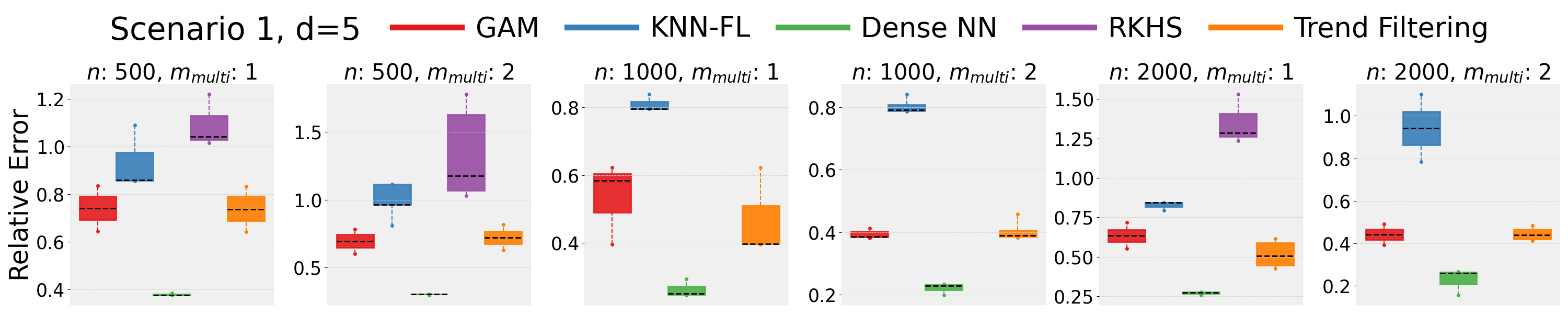
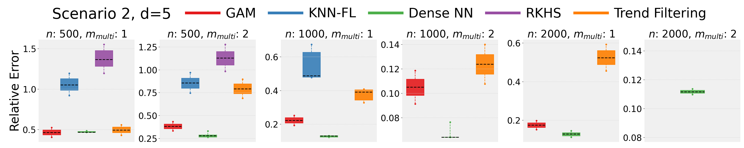
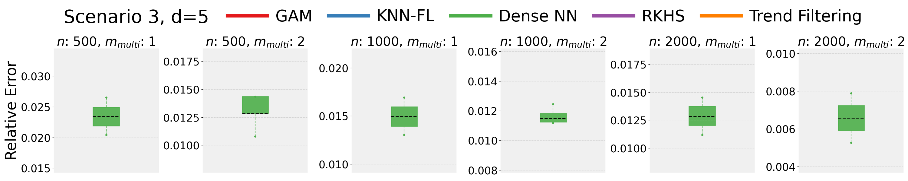
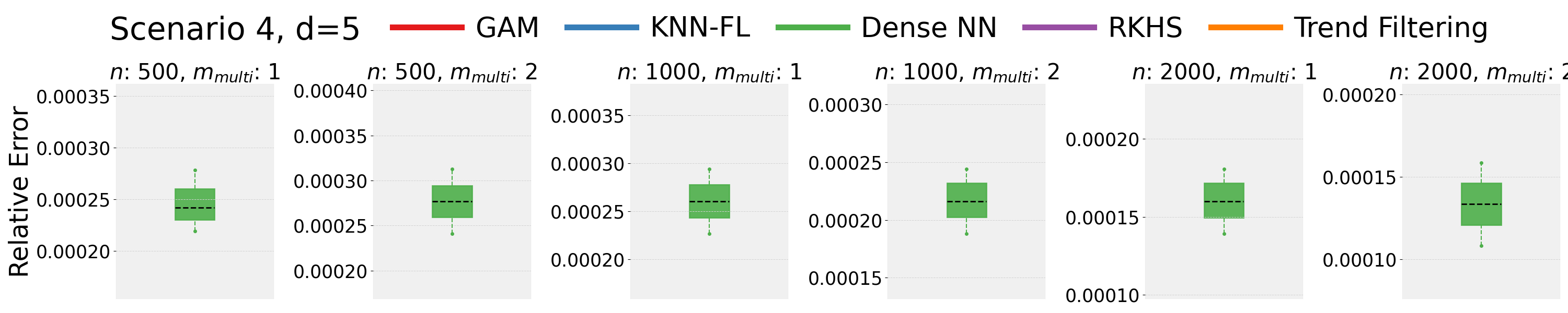
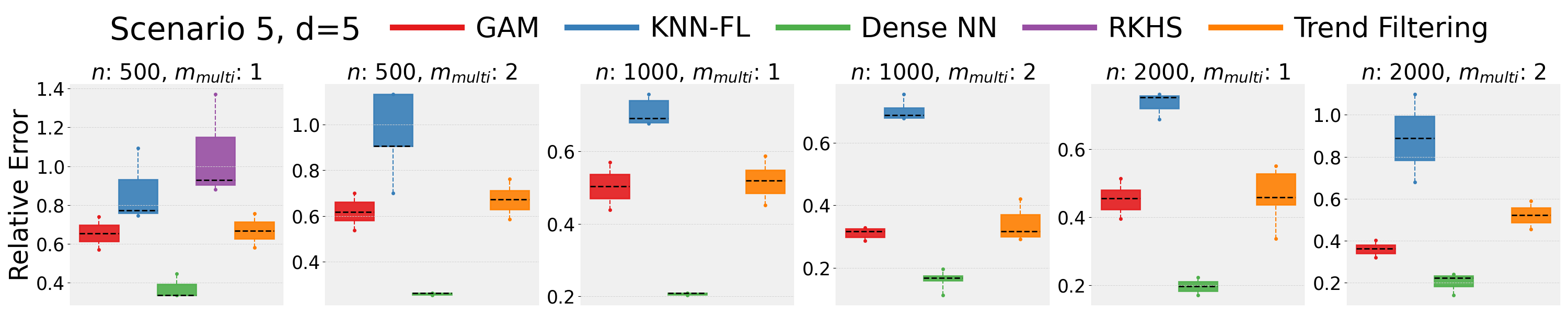
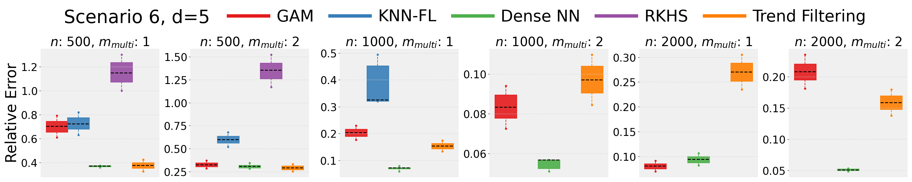
Figure 9: Comparison of methods across different scenarios, $d=5$, $n$, and $m_{mult}$ by box-plot. For each $(n,m_{mult})$ setting, we present the errors of the competitors in the range of within 5 times the smallest error.

Table 5: Hyperparameters for Dense NN Selected by $5$-fold Cross-validation

Hyperparameter	Scenario
	1	2	3	4	5	6
L $\in\{1,2,3,4,5,10\}$ (Layers)	3	5	4	2	5	2
N $\in\{30,60,100,300\}$ (Neurons)	60	30	100	60	30	30

Table 6: Hyperparameters for GAM Selected by $5$-fold Cross-validation

Hyperparameter	Scenario
	1	2	3	4	5	6
basis $\{\text{'ps': p-spline basis, 'cp': cyclic p-spline basis}\}$ (Basis Type)	ps	ps	ps	ps	ps	ps
constraint $\{\text{None, 'convex', 'concave', \noindent\hbox{}\hfill{{\hbox{\begin{tabular}[c]{@{}c@{}}mono\\ inc\end{tabular}}}}\hfill\hbox{}, \noindent\hbox{}\hfill{{\hbox{\begin{tabular}[c]{@{}c@{}}mono\\ dec\end{tabular}}}}\hfill\hbox{}}\}$ (Constraint Type)	mono dec	mono dec	convex	None	mono dec	mono inc
$\lambda$, with $\log_{10}(\lambda)\in[-3,3]$ (Regularization Parameter)	63.1	0.001	0.25	3.98	1000	0.015
n_splines $\in\{6,7,8,9,10\}$ (Number of Splines)	7	8	9	6	6	7
spline $\in\{1,2,3,4,5\}$ (Spline Order)	1	1	2	4	5	5

Table 7: Hyperparameters for KNN-FL Selected by $5$-fold Cross-validation

Hyperparameter	Scenario
	1	2	3	4	5	6
lambda $\in\{0.00001,0.0001,0.01,0.1,1,10,100\}$ (Regularization Parameter)	0.01	0.01	0.00001	0.0001	0.01	0.01
n_neighbors $\in\{5,10\}$ (Number of Neighbors)	10	10	5	5	5	5

Table 8: Hyperparameters for RKHS Selected by $5$-fold Cross-validation

Hyperparameter	Scenario
	1	2	3	4	5	6
$\alpha$, with $\log_{10}(\alpha)\in[-2,2]$ (Regularization Parameter)	100	100	100	100	100	100
kernel$\in\{\text{polynomial, laplacian, linear}\}$ (Kernel Type)	polynomial	polynomial	laplacian	polynomial	polynomial	laplacian

Table 9: Hyperparameters for Trend Filtering Selected by $5$-fold Cross-validation

Hyperparameter	Scenario
	1	2	3	4	5	6
$k\in\{0,1,2\}$ (Trend Order)	1	0	1	0	1	1
lambda, $\log_{10}(\lambda)\in[-5,2]$ (Regularization Parameter)	0.0007	0.8133	0.0001	0.1128	7.8476	0.6158

References

- Bartlett et al. (2019) Peter L Bartlett, Nick Harvey, Christopher Liaw, and Abbas Mehrabian. Nearly-tight vc-dimension and pseudodimension bounds for piecewise linear neural networks. The Journal of Machine Learning Research, 20(1):2285–2301, 2019.
- Bauer and Kohler (2019) Benedikt Bauer and Michael Kohler. On deep learning as a remedy for the curse of dimensionality in nonparametric regression. The Annals of Statistics, 47(4):2261 – 2285, 2019. doi: 10.1214/18-AOS1747. URL https://doi.org/10.1214/18-AOS1747.
- Belkin and Niyogi (2003) Mikhail Belkin and Partha Niyogi. Laplacian eigenmaps for dimensionality reduction and data representation. Neural computation, 15(6):1373–1396, 2003.
- Boucheron et al. (2013) Stéphane Boucheron, Gábor Lugosi, and Pascal Massart. Concentration Inequalities: A Nonasymptotic Theory of Independence. Oxford University Press, 02 2013. ISBN 9780199535255. doi: 10.1093/acprof:oso/9780199535255.001.0001. URL https://doi.org/10.1093/acprof:oso/9780199535255.001.0001.
- Cai and Hall (2006) T Tony Cai and Peter Hall. Prediction in functional linear regression. 2006.
- Cai and Yuan (2012) T Tony Cai and Ming Yuan. Minimax and adaptive prediction for functional linear regression. Journal of the American Statistical Association, 107(499):1201–1216, 2012.
- Cardot et al. (1999) Hervé Cardot, Frédéric Ferraty, and Pascal Sarda. Functional linear model. Statistics & Probability Letters, 45(1):11–22, 1999.
- Cardot et al. (2003) Hervé Cardot, Frédéric Ferraty, André Mas, and Pascal Sarda. Testing hypotheses in the functional linear model. Scandinavian Journal of Statistics, 30(1):241–255, 2003.
- Chambolle and Darbon (2009) Antonin Chambolle and Jérôme Darbon. On total variation minimization and surface evolution using parametric maximum flows. International journal of computer vision, 84(3):288–307, 2009.
- Chen et al. (2022) Minshuo Chen, Haoming Jiang, Wenjing Liao, and Tuo Zhao. Nonparametric regression on low-dimensional manifolds using deep relu networks: Function approximation and statistical recovery. Information and Inference: A Journal of the IMA, 11(4):1203–1253, 2022.
- Cloninger and Klock (2021) Alexander Cloninger and Timo Klock. A deep network construction that adapts to intrinsic dimensionality beyond the domain. Neural Networks, 141:404–419, 2021.
- Cover (1968) Thomas M Cover. Rates of convergence for nearest neighbor procedures. In Proceedings of the Hawaii International Conference on Systems Sciences, volume 415, 1968.
- Donoho (2000) David L Donoho. High-dimensional data analysis: The curses and blessings of dimensionality. AMS Math Challenges Lecture, 2000.
- Doukhan (2012) Paul Doukhan. Mixing: properties and examples, volume 85. Springer Science & Business Media, 2012.
- Glorot et al. (2011) Xavier Glorot, Antoine Bordes, and Yoshua Bengio. Deep sparse rectifier neural networks. In Proceedings of the fourteenth international conference on artificial intelligence and statistics, pages 315–323. JMLR Workshop and Conference Proceedings, 2011.
- Goodfellow et al. (2014) Ian Goodfellow, Jean Pouget-Abadie, Mehdi Mirza, Bing Xu, David Warde-Farley, Sherjil Ozair, Aaron Courville, and Yoshua Bengio. Generative adversarial nets. Advances in neural information processing systems, 27, 2014.
- Graves and Graves (2012) Alex Graves and Alex Graves. Long short-term memory. Supervised sequence labelling with recurrent neural networks, pages 37–45, 2012.
- Györfi et al. (2002) László Györfi, Michael Köhler, Adam Krzyżak, and Harro Walk. A distribution-free theory of nonparametric regression, volume 1. Springer, 2002.
- Hall and Horowitz (2007) Peter Hall and Joel L Horowitz. Methodology and convergence rates for functional linear regression. 2007.
- Hastie et al. (2009) Trevor Hastie, Robert Tibshirani, and Jerome Friedman. The Elements of Statistical Learning: Data Mining, Inference, and Prediction. Springer, New York, 2009.
- Hofmann et al. (2008) Thomas Hofmann, Bernhard Schölkopf, and Alexander J Smola. Kernel methods in machine learning. 2008.
- Jiao et al. (2023) Yuling Jiao, Guohao Shen, Yuanyuan Lin, and Jian Huang. Deep nonparametric regression on approximate manifolds: Nonasymptotic error bounds with polynomial prefactors. The Annals of Statistics, 51(2):691–716, 2023.
- Kohler and Langer (2019) Michael Kohler and Sophie Langer. On the rate of convergence of fully connected very deep neural network regression estimates. arXiv preprint arXiv:1908.11133, 2019.
- Kohler et al. (2023) Michael Kohler, Sophie Langer, and Ulrich Reif. Estimation of a regression function on a manifold by fully connected deep neural networks. Journal of Statistical Planning and Inference, 222:160–181, 2023.
- Krizhevsky et al. (2017) Alex Krizhevsky, Ilya Sutskever, and Geoffrey E Hinton. Imagenet classification with deep convolutional neural networks. Communications of the ACM, 60(6):84–90, 2017.
- Kühn and Schilling (2023) Franziska Kühn and René L Schilling. Maximal inequalities and some applications. Probability Surveys, 20:382–485, 2023.
- Lawson (2013) Andrew B Lawson. Statistical methods in spatial epidemiology. John Wiley & Sons, 2013.
- Ma and Safikhani (2022) Mingliang Ma and Abolfazl Safikhani. Theoretical analysis of deep neural networks for temporally dependent observations. Advances in Neural Information Processing Systems, 35:37324–37334, 2022.
- Nair and Hinton (2010) Vinod Nair and Geoffrey E Hinton. Rectified linear units improve restricted boltzmann machines. In Proceedings of the 27th international conference on machine learning (ICML-10), pages 807–814, 2010.
- Padilla et al. (2018) Oscar Hernan Madrid Padilla, James Sharpnack, Yanzhen Chen, and Daniela M Witten. Adaptive non-parametric regression with the -nn fused lasso. arXiv preprint arXiv:1807.11641, 2018.
- Petersen and Müller (2016) Alexander Petersen and Hans-Georg Müller. Functional data analysis for density functions by transformation to a hilbert space. 2016.
- Radford (2018) A Radford. Improving language understanding by generative pre-training. 2018.
- Ramdas and Tibshirani (2016) Aaditya Ramdas and Ryan J Tibshirani. Fast and flexible admm algorithms for trend filtering. Journal of Computational and Graphical Statistics, 25(3):839–858, 2016.
- Rosasco et al. (2004) Lorenzo Rosasco, Tomaso Poggio, Ernesto D Vito, and Andrea Caponnetto. Are loss functions all the same? Neural Computation, 16(5):1063–1076, 2004.
- Roweis and Saul (2000a) Sam T Roweis and Lawrence K Saul. Nonlinear dimensionality reduction by locally linear embedding. Science, 290(5500):2323–2326, 2000a.
- Roweis and Saul (2000b) ST Roweis and LK Saul. Nonlinear dimensionality reduction by locally linear embedding. Science, 290(5500):2323–2326, 2000b.
- Sadhanala and Tibshirani (2019) Veeranjaneyulu Sadhanala and Ryan J Tibshirani. Additive models with trend filtering. The Annals of Statistics, 47(6):3032–3068, 2019.
- Schmidt-Hieber (2020) Johannes Schmidt-Hieber. Nonparametric regression using deep neural networks with relu activation function. 2020.
- Sharma et al. (2017) Sagar Sharma, Simone Sharma, and Anidhya Athaiya. Activation functions in neural networks. Towards Data Sci, 6(12):310–316, 2017.
- Stone (1982) Charles J Stone. Optimal global rates of convergence for nonparametric regression. The annals of statistics, pages 1040–1053, 1982.
- Stone (1985) Charles J Stone. Additive regression and other nonparametric models. The annals of Statistics, 13(2):689–705, 1985.
- Stone (1994) Charles J Stone. The use of polynomial splines and their tensor products in multivariate function estimation. The annals of statistics, 22(1):118–171, 1994.
- Taigman et al. (2014) Yaniv Taigman, Ming Yang, Marc’Aurelio Ranzato, and Lior Wolf. Deepface: Closing the gap to human-level performance in face verification. In Proceedings of the IEEE conference on computer vision and pattern recognition, pages 1701–1708, 2014.
- Tenenbaum et al. (2000a) JB Tenenbaum, V De Silva, and JC Langford. A global geometric framework for nonlinear dimensionality reduction. Science, 290(5500):2319–2323, 2000a.
- Tenenbaum et al. (2000b) Joshua B Tenenbaum, Vin De Silva, and John C Langford. A global geometric framework for nonlinear dimensionality reduction. Science, 290(5500):2319–2323, 2000b.
- Tian et al. (2021) Peng Tian, Jialin Li, Luodan Cao, Ruiliang Pu, Zhongyi Wang, Haitao Zhang, Huilin Chen, and Hongbo Gong. Assessing spatiotemporal characteristics of urban heat islands from the perspective of an urban expansion and green infrastructure. Sustainable Cities and Society, 74:103208, 2021.
- Vaswani (2017) A Vaswani. Attention is all you need. Advances in Neural Information Processing Systems, 2017.
- Wikle et al. (2019) Christopher K Wikle, Andrew Zammit-Mangion, and Noel Cressie. Spatio-temporal statistics with R. CRC Press, 2019.
- Wood (2017) Simon N Wood. Generalized additive models: an introduction with R. chapman and hall/CRC, 2017.
- Wu et al. (2021) Rong Wu, Zhigang Li, and Shaojian Wang. The varying driving forces of urban land expansion in china: Insights from a spatial-temporal analysis. Science of The Total Environment, 766:142591, 2021.