A Secure Estimator with Gaussian
Bernoulli Mixture Model

Abstract

The implementation of cyber-physical systems in real-world applications is challenged by safety requirements in the presence of sensor threats. Most cyber-physical systems, in particular the vulnerable multi-sensor systems, struggle to detect the attack in observation signals. In this paper, we tackle this issue by proposing a Gaussian-Bernoulli Secure (GBS) estimator, which effectively transforms the assessment of sensor status into an optimal estimation problem concerning the system state and observation indicators. It encompasses two theoretical sub-problems: sequential state estimation with partial observations and estimation updates with disordered new observations. Within the framework of Kalman filter, we derive closed-form solutions for these two issues. However, due to their computational inefficiency, we propose the iterative approach employing proximal gradient descent to accelerate the estimation update. We conduct comprehensive experiments from three perspectives: computational efficiency, detection and estimation performance, and characterization of observation error. Our GBS estimator shows the improvements compared to other methods.

I Introduction

Cyber-Physical Systems (CPSs) are integrative frameworks that combine computing and communication capabilities to monitor or control entities within the physical world [1][2]. Over the past two decades, significant advancements in communication and computing technologies have catalyzed the wide applications for CPSs [3]. The advancement in wireless communication technologies has enabled CPSs to transmit real-time signals across expansive physical networks [4]. Furthermore, armed with advanced computational resources, CPS can optimize control strategies for complex systems online in real-time  [5]. This technological evolution broadens the scope of CPSs, impacting various sectors such as medical devices [6], smart grids [7], and autonomous vehicles [8].

However, alongside the opportunities, CPSs face significant challenges, with security issues emerging as a paramount concern. A notable incident underscoring this concern involves the RQ-170, an American drone [9][10], which lost control in Iran due to a security breach. This security breach was executed through the manipulation of the drone’s GPS signal, causing the UAV to land in a strategically targeted area. The reliance of many CPSs on remote signal transmission over vulnerable networks opens them up to sensory attacks. These attacks, through the injection of malicious data [11] or disruption of information transmission [12], can significantly degrade a system’s performance, e.g., maximizing the estimation error covariance [13], amplifying the expected estimation error [14].

Against various sensory attacks, two types of detection methods are widely studied. One is the model-based defense mechanisms, e.g., control theory, game theory and cryptography. Detectors based on linear estimation theory, which analyze the Kalman innovation sequence, are widely applied in CPS, especially windows $\chi^{2}$ detector [15], CUSUM detector [16] and MEWMA detector [17]. The framework of game theory also enables the design of the optimal defense policies. For instance, Basar et al. [5] considered the system balance between resilience and robustness, Li et al. [18] obtained the optimal DoS defense strategy by solving the associated Bellman equations, and Meira-Góes et al. [19] improved the efficiency of synthesized robust supervisors against sensor deception attacks. Additionally, with the idea of cryptography, Mo et al. [20] proposed the watermarking approach to authenticate the correct operation of a control system, while Kogiso et al. [21] incorporated the public key encryption scheme into the design of remote controller or observers. Another strategy involves using learning-based methods to identify CPS attacks. The graph neural network (GNN) approach proposed in [22] provided a solution for interpretation and localization of anomalies in secure water treatment, overcoming the challenges of high dimensionality and complexity. Besides, LSTM-RNNs were applied in [23] for learning the temporal behaviour of the data in CPSs and identifying sensor anomalies. Moreover, Wang et al. [24] utilized Deep Belief Network (DBF) to train an interval state predictor for pattern recognition in sensor security.

Apart from detecting attacks, designing resilient state estimators played a critical role in mitigating sensor attacks. Mo et al. [25] studied the case of multiple measurements subject to sensor attacks, designing an optimal estimator by solving a minimax optimization problem. In addition, regarding secure estimation problem in noiseless systems, Chang et al. [26] formulated it as the classical error correction problem and provided the sufficient conditions for restoring the real states. Furthermore, Wang et al. [27] considered attacked sensor signals as general outliers, obtaining resilient estimates by identifying and eliminating these outliers. Previous detecting methods have two limitations. First, attack detectors and resilient state estimators are interdependently designed and the connection between them are overlooked. It is challenging to ensure the estimation performance while simultaneously detecting attacks. Second, occasional outliers and persistent malicious attacks are difficult to distinguish, as their Kalman innovation sequences may overlap. If we can separate these outliers from observations, the binary detection problem will become more accurate, thereby reducing the false alarm rate.

To overcome these shortcomings, we initiatively formulate the potential anomalies and normal Gaussian noise as a Gaussian-Bernoulli mixture model by introducing observation indicators. By solving a dual-variable estimation problem, our proposed algorithm can simultaneously achieves resilient state estimation and attack detection. The main contributions of this article include:

1. We introduce, for the first time, the Gaussian-Bernoulli mixture model to model the observation model with potential attack risks. Under the mixture model, we propose a novel framework to integrate the attack detection and resilient estimation into a dual-variable optimization problem.

2. Within the framework of Kalman filter and RTS smoother, we derive analytical solutions for two subproblems: sequential state estimation with partial observations and estimation update with disordered new observations.

3. We propose an innovative iterative method that addresses the challenge of non-sequential observation changes. By using the previous estimation as the initial point and employing proximal gradient descent, it rapidly converges to the optimal estimation with updated observations.

4. We test the performance of the GBS estimator under various types and intensities of attacks, and observe a significant improvement compared to previous algorithms.

The remainder of the paper is organized as follows. In Section II, we introduce the linear estimation as an application of Bayesian theory in Hidden Markov Chains. In Section III, we describe the model assumptions and the problem we aim to solve. In Sections IV and V, we discuss the core step of our algorithm: updating the state sequence estimation in response to disordered changes in the observation set. In Section VI, we propose our Gaussian-Bernoulli secure estimator and prove its convergence. In Section VII, we demonstrate our algorithm’s performance and compare it with other algorithms. In Section VIII, we conclude the paper. For clarity, this paper focuses on the single-sensor system, but the derivation process and conclusions are also applicable to multi-sensor systems.

Notation: For $S\in R^{n\times n},S\succ 0$, let $\|x\|_{S}=\sqrt{x^{T}Sx}$ denoting the S-weighted 2-norm of $x$. Denote the state sequence at interval $T=[0,N]$ as $x_{0:N}=\{x_{0},\cdots,x_{N}\}$. The observation set is denoted as $y_{0:N}=\{y_{0},\cdots,y_{N}\}$. The observation indicators are denoted as $p_{0:N}=\{p_{0},\cdots,p_{N}\}$. Let $\mathcal{O}\in 2^{\{0,\cdots,N\}}$ denotes the selected index set, and then $y_{\mathcal{O}}$ denotes the selected observation set. $\hat{x}_{i|\mathcal{O}}$ denotes the optimal estimation of the state $x_{i}$ under the observation set $y_{\mathcal{O}}$. Let symbol $\circ$ denoting the composition of functions.

II Bayes’ theorem in HMMs

This section introduces Bayesian estimation as tools for analyzing stochastic systems and estimating the states of a hidden Markov model (HMM). Furthermore, we present the steps of Kalman filter and RTS smoother, highlighting their optimality within the theoretical framework.

II-A Bayesian estimation

Bayesian estimation is a statistical inference method for updating the beliefs in presence of new evidence. This approach is particularly useful where data is limited or uncertainty is high.

At the heart of Bayesian estimation is Bayes’ theorem, which describes the relationship between conditional probabilities. It applies the concepts of probability to the random variables and their relations, including the prior probability $p(x)$, likelihood function $p(y|x)$ and posterior probability $p(x|y)$. The theorem can be expressed as:

$$p(x|y)=\frac{p(y|x)\cdot p(x)}{p(y)}$$

where $p(x)$ represents current knowledge before observation, $p(y|x)$ describes the known statistical model of observation given the state, and $p(x|y)$ updates probability of the state after observation.

The Minimum Mean Squared Error (MMSE) and Maximum A Posteriori (MAP) are two classic Bayesian estimation methods, each with different probabilistic optimization objectives.

II-A1 MMSE

In the Bayesian framework, the goal of MMSE estimation is to minimize the mean squared error between the estimated values and the true values. Mathematically, the MMSE estimator can be expressed as:

$$\hat{x}^{\text{MMSE}}=\arg\min_{\hat{x}}\mathbf{E}[\|x-\hat{x}\|^{2}|y]$$

Further, when the posterior distribution is symmetric without the heavy tail, the MMSE estimator is equal to the expectation under certain conditions.

$$\hat{x}^{\text{MMSE}}=\mathbf{E}[x|y]=\int x\cdot p(x|y)~{}dx=\int x\cdot\frac{p(y|x)\cdot p(x)}{p(y)}dx$$

The MMSE estimator focuses on minimizing the overall error, providing an estimate that performs best on average across all possible values.

II-A2 MAP

The MAP estimator aims to find the state value that maximizes the posterior probability. It means that given the observed data, we seek the state value most likely to produce these data. Mathematically, the MAP estimator can be expressed as:

$$\hat{x}^{\text{MAP}}=\arg\max_{\hat{x}}p(\hat{x}|y)=\arg\max_{\hat{x}}\frac{p(y|\hat{x})\cdot p(\hat{x})}{p(y)}$$

MAP estimator aims to determine the most probable parameter value, providing a more convicing estimate when the random variables are discrete.

II-B Kalman filter and RTS smoother

The Kalman filter can be considered as a specific application of Bayesian estimation in HMMs. The uniqueness of the Kalman filter is reflected in three main aspects.

First, both state transitions and observation processes are assumed to be linear and accompanied by Gaussian noise. They can be expressed as:

$$x_{t+1}\sim\mathcal{N}(A{x}_{t},Q)$$

$$y_{t}\sim\mathcal{N}(C{x}_{t},R)$$

where $Q>0$ and $R>0$ denotes the process noise and observation noise. The probability density function of $\mathcal{N}(\mu,\Sigma)$ is given by the following formula

$$p(x)\propto\exp\left(-\frac{1}{2}\|x-\mu\|^{2}_{\Sigma^{-1}}\right).$$

Additionally, the minimal estimation error obtained by MMSE has a linear relationship with the observation and process error. Therefore, given the system state $x_{t}\sim\mathcal{N}(\hat{x}_{t|t}^{*},P_{t|t})$, when a new observation $y_{t+1}$ is made, the linear MMSE (LMMSE) estimator and MAP estimator will infer $\hat{x}_{t+1}$ and adjust $\hat{x}_{t}$ by solving different optimization problems.

LMMSE

$$\hat{x}^{\text{LMMSE}}_{t+1},K=\begin{array}[]{cl}\displaystyle\arg&\min_{\hat{x}_{t+1},K}E[\|x_{t+1}-\hat{x}_{t+1}\|^{2}]\\ \textrm{s.t.}&\hat{x}_{t+1}=A\hat{x}_{t|t}^{*}+K(y_{t+1}-CA\hat{x}_{t|t}^{*})\end{array}$$

$$\hat{x}^{\text{LMMSE}}_{t},F=\begin{array}[]{clll}\displaystyle\arg&\min_{\hat{x}_{t},F}E[\|x_{t}-\hat{x}_{t}\|^{2}]\\ \textrm{s.t.}&\hat{x}_{t}=A\hat{x}_{t|t}^{*}+F(\hat{x}^{\text{LMMSE}}_{t+1}-A\hat{x}_{t|t}^{*})\end{array}$$

MAP

$$\hat{x}^{\text{MAP}}_{t+1},\hat{x}^{\text{MAP}}_{t} =\arg\max_{\hat{x}_{t+1},\hat{x}_{t}}~{}p(\hat{x}_{t+1},\hat{x}_{t}|y_{t+1})$$

$$=\arg \max_{\hat{x}_{t+1},\hat{x}_{t}}~{}p(y_{t+1}|\hat{x}_{t+1})p(\hat{x}_{t+1}|\hat{x}_{t})p(\hat{x}_{t}|x_{t})$$

$$=\arg \min_{\hat{x}_{t+1},\hat{x}_{t}}~{}[\|y_{t+1}-C\hat{x}_{t+1}\|^{2}_{R^{-1}}+$$

$$\|\hat{x}_{t+1}-A\hat{x}_{t}\|^{2}_{Q^{-1}}+\|\hat{x}_{t}-\hat{x}_{t|t}^{*}\|^{2}_{P_{t|t}^{-1}}]$$

Moreover, LMMSE and MAP have the same result in linear Gaussian model. The closed-form solution of optimal estimate can be calculated by Kalman filter and Rauch-Tung-Striebel (RTS) smoother, respectively.

$$\hat{x}_{t+1|t+1}=\hat{x}^{\text{LMMSE}}_{t+1}=\hat{x}^{\text{MAP}}_{t+1}$$

$$\hat{x}_{t|t+1}=\hat{x}^{\text{LMMSE}}_{t}=\hat{x}^{\text{MAP}}_{t}$$

Kalman filter

$$\hat{x}_{t+1|t} =A\hat{x}_{t|t}$$

$$P_{t+1|t} =AP_{t|t}A^{T}+Q$$

$$K_{t+1} =P_{t+1|t}C^{T}(CP_{t+1|t}C^{T}+R)^{-1}$$

$$r_{t+1} =y_{t+1}-C\hat{x}_{t+1|t}$$

$$\hat{x}_{t+1|t+1} =\hat{x}_{t+1|t}+K_{t+1}r_{t+1}$$

$$P_{t+1|t+1} =(I-K_{t+1}C)P_{t+1|t}$$

RTS smoother

$$F_{t} =P_{t|t}A^{T}P_{t+1|t}^{-1}$$

$$\hat{x}_{t|t+1} =\hat{x}_{t|t}+F_{t}(\hat{x}_{t+1|t+1}-A\hat{x}_{t|t})$$

$$P_{t|t+1} =P_{t|t}+F_{t}(P_{t+1|t+1}-P_{t+1|t})F_{t}^{T}$$

III problem formulation

This section introduces the Gaussian-Bernoulli mixture observation model and explains its motivation. Following this, we describe our objectives and formulate them as a dual-variable optimization problem involving state estimation and Boolean decision-making. To avoid unnecessary complexity, we describe the problem under a single sensor scenario.

III-A System model

We consider a linear time-invariant system with process and measurement noise:

$$\left\{\begin{matrix}x_{t+1}&=&Ax_{t}+w_{t}\\ y_{t}&=&Cx_{t}+\bar{v}_{t}\end{matrix}\right.$$ (1)

where the system state $x_{t}\in\mathbf{R}^{n}$, the measurement $y_{t}\in\mathbf{R}^{m}$ and the pair $(A,C)$ is observable. We assume the process noise $\{w_{t}\}$ satisfies i.i.d Gaussian distribution $\mathcal{N}(0,Q)$, and is not uncorrelated with measurement noise $\{\bar{v}_{t}\}$, which is non-Gaussian, especially when under attack.

Significantly, reducing the false alarm rate of detectors is the motivation for not using the standard Gaussian model to describe observations. In most of paper, the probability of observing low-probability events is ignored by Gaussian model, even though their real distribution is crucial for determining whether an attack has occurred. To tackle it, we consider a more general model:

$$\bar{v}_{t}=v_{t}+\Delta v_{t}$$ (2)

where $\{v_{t}\}$ has Gaussian distribution, and $\{\Delta v_{t}\}$ denotes the discrepancy between the real noise and the fitted Gaussian distribution, including outliers and malicious sensor attacks.

The challenge is how to model $\Delta v_{t}$. There are two intuitions for modeling $\Delta v_{t}$. One is that the fitting error between $v_{t}$ and the real sample data is relatively uniform across different values. Another motivation is that it is difficult to accurately characterize the distribution of large error events, but it is straightforward to use a Bernoulli distribution to describe the likelihood of one of large error events occurring.

Assumption 1.

The measurement noise $\{\bar{v}_{t}\}$ is expressed as a Gaussian-Bernoulli mixture model:

$$\bar{v}_{t}=v_{t}+\Delta v_{t}=v_{t}+p_{t}*\delta_{t}$$ (3)

where $\{v_{t}\}$ has Gaussian ditribution $\mathcal{N}(0,R)$, $\{p_{t}\}$ has Bernoulli distribution $\mathcal{B}(N,\beta)$, and $\{\delta_{t}\}$ has uniform distribution with unknown probability density. Random variables $\{p_{t}\},\{\delta_{t}\},\{v_{t}\}$ are uncorrelated with each other.

This mixture model can be interpreted as conforming to a Gaussian distribution in most cases with occasional unknown distribution. We name the $\{p_{t}\}$ as observation indicators.

III-B Problem description

Our goal is to design a secure detector to determine whether the observation sequence of fixed length $N$ is reliable. The secure detector operates in parallel with the estimator that updates the state estimation. In other words, at a certain moment, the secure detector can use the observations before and after to determine whether it is reliable.

Suppose that the system’s observation model conforms to Assumption 1. Without loss of generality, we assume the detector knows the distribution of the initial state $x_{0}\sim\mathcal{N}(0,P_{0}),P_{0}>0$. To determine whether sensors have suffered attacks at interval $T=[0,N]$, the detector rechecks the observation sequences and evaluates the reliability of the sensors.

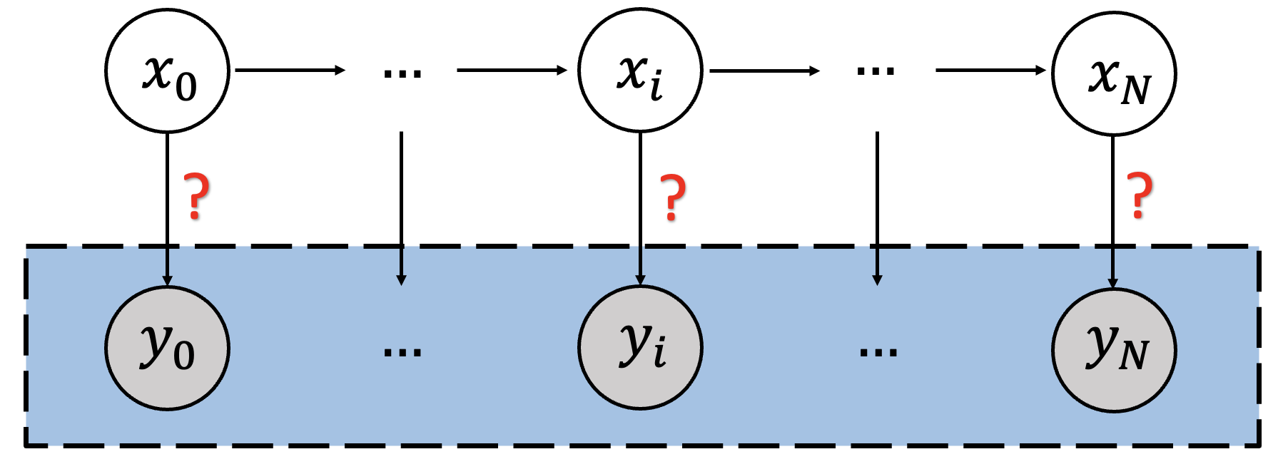
Figure 1: Illustration of the detection problem under sensor attacks.

For each sensor, the evaluation of the observation sequence relies on the inference of each observation. Under Assumption 1, $y_{t}$ is considered normal when $p_{t}=0$, as the observation noise conforms to a Gaussian distribution; whereas when $p_{t}=1$, the observation noise is with unknown distribution, which is considered abnormal. Based on the $0-1$ sequence of observation indicators $p_{0:N}$, we can classify the observation sequence into three status with threshold $\tau$: in normal case, with general outliers, or under malicious sensor attacks.

$\{p_{0},\cdots,p_{N}\}$	$\sum_{i=0}^{N}p_{t}$	the status of observation sequence
$0,0,0,\cdots,0$	0	in normal case
$0,1,0,\cdots,0$ $\dots$	$\leq\tau$	with general outliers
$\dots$ $1,1,1,\cdots,1$	$>\tau$	under sensor attacks

The primary issue is how to estimate the indicator sequence $\hat{p}_{0:N}$ through the observation sequence $y_{0:N}$. If we know $x_{t}$ and $p_{t}\sim\mathcal{B}(1,\beta)$, we can infer $\hat{p}_{t}$ by comparing the posterior probabilities of $p_{t}=0$ and $p_{t}=1$,

$$\max_{\hat{\delta}_{t}}P(p_{t}=0,\hat{\delta}_{t}|y_{t})= \exp\left(-\frac{1}{2}\|y_{t}-C{x}_{t}\|^{2}_{R^{-1}}\right)$$

$$\cdot(1-\beta)\cdot p({\delta}_{t}^{1})$$ (4)

$$\max_{\hat{\delta}_{t}}P(p_{t}=1,\hat{\delta}_{t}|y_{t})\ = \exp\left(0\right)\cdot\beta\cdot p({\delta}_{t}^{2})$$ (5)

Because ${\delta}_{t}$ follows a uniform distribution, inferring the value of $p_{t}$ is equivalent to solving the following optimization problem:

$$\arg\min_{\hat{p}_{t}\in\{0,1\}}~{}\left\{(1-\hat{p}_{t})\|y_{t}-C{x}_{t}\|^{2}_{R^{-1}}+\alpha\hat{p}_{t}\right\}$$ (6)

where $\alpha\propto\ln{(\frac{1-\beta}{\beta})}$ is a constant value calculated by the $\beta$ in Bernoulli distribution.

Estimating $\{x_{t}\}$ is a prerequisite for estimating $\{p_{t}\}$, and thus another core issue is how to obtain the optimal estimation of $\hat{x}_{0:N}$ through $y_{0:N}$. The distribution of noise is partially known under Assumption 1, hence the result of the classical Kalman filter is no longer the optimal estimation. However, if we neglect those observations with unknown distribution, the state estimation can still be calculated based on those reliable observations $\{y_{t}|p_{t}=0\}$.

The problems of obtaining $\{\hat{p}_{t}\}$ and $\{\hat{x}_{t}\}$ are coupled. A reliable detector relies on accurate state estimator, while at the same time, effective elimination of anomalies contributes to better estimation performance. Consequently, we formulate it to a dual-variable optimization problem

Problem 1

$$\arg\min_{\hat{x}_{0:N},\hat{p}_{0:N}}~{}\mathcal{W} (\hat{x}_{0:N},\hat{p}_{0:N})=\Biggl{\{}\sum_{i=0}^{N}[(1-\hat{p}_{i})\|y_{i}-C\hat{x}_{i}\|^{2}_{R^{-1}}$$

$$+\alpha\hat{p}_{i}]+ \sum_{i=1}^{N}\|\hat{x}_{i}-A\hat{x}_{i-1}\|^{2}_{Q^{-1}}+\|\hat{x}_{0}\|^{2}_{P_{0}^{-1}}\Biggr{\}}$$ (7)

It is a Mixed-Integer Programming (MIP) problem with a mix of continuous variables ($\hat{x}_{0:N}$) and Boolean variables ($\hat{p}_{0:N}$). Solving such problem is challenging due to the non-convex nature of the objective function and the combinatorial complexity introduced by integer variables.

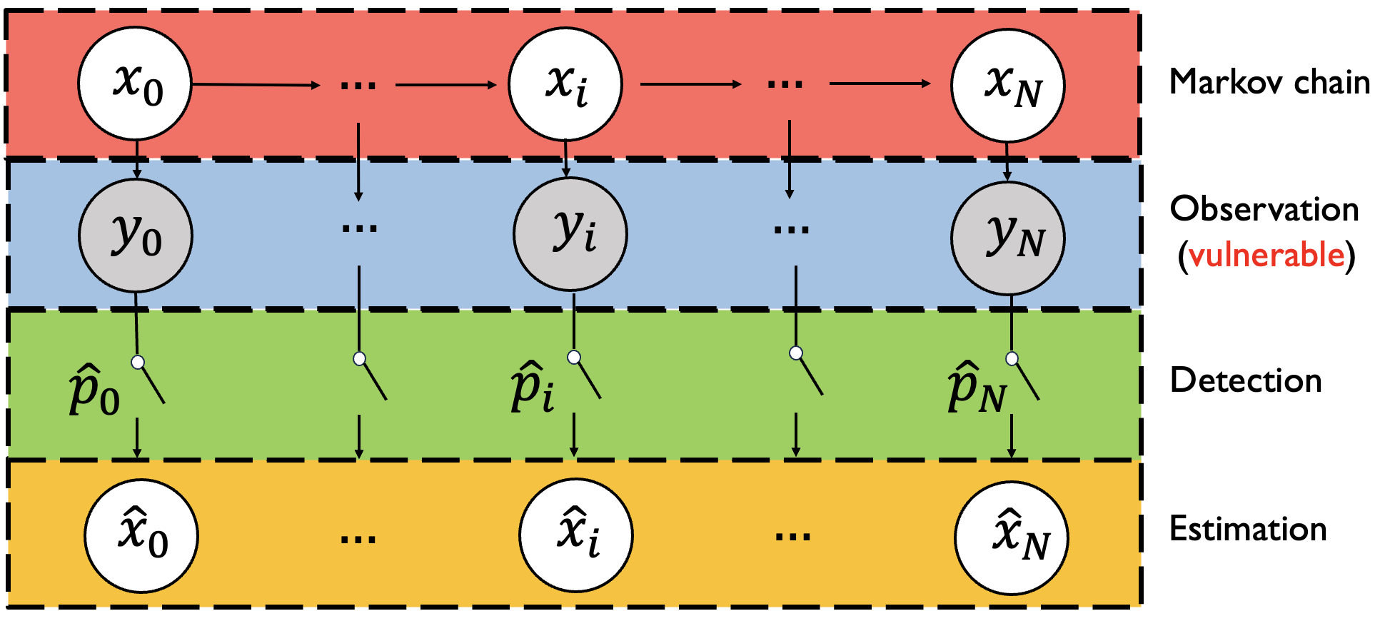
Figure 2: Illustration of the MIP problem. The red color represents the real system states in HMM. The blue color represents the observation sequence, which may contain unreliable data. The green color indicates the determination of the observation reliability in MIP problem. The yellow color signifies that it simultaneously estimate the system states with reliable observations.

IV Direct approach for state estimation

In this section, we solve a special case of Problem 1. When the observation indicators are fixed, what is the closed-form solution of equation (7)? Furthermore, when observation indicators changes, how should the solution of equation (7) be updated? These are the two key steps of our algorithm.

When $\hat{p}_{0:N}$ is fixed, let us define the selected index set $\mathcal{O}=\{i|\hat{p}_{i}=0\}$. Problem 1 degenerates into the following problem.

Problem 2

$$\arg\min_{\hat{x}_{0:N}}~{}\mathcal{L}_{\mathcal{O}} (\hat{x}_{0:N})=\Biggl{\{}\sum_{i\in\mathcal{O}}\|y_{i}-C\hat{x}_{i}\|^{2}_{R^{-1}}$$

$$+ \sum_{i=1}^{N}\|\hat{x}_{i}-A\hat{x}_{i-1}\|^{2}_{Q^{-1}}+\|\hat{x}_{0}\|^{2}_{P_{0}^{-1}}\Biggr{\}}$$ (8)

The optimization objective of equation (8) corresponds to a MAP state estimation problem. This problem can be translated into the following question. The goal is to estimate the state sequence $x_{0:N}$ based on a partial observation set $y_{\mathcal{O}}=\{y_{i}\mid i\in\mathcal{O}\}$, where $y_{\mathcal{O}}\subseteq y_{0:N}$, in which the measurement errors follow a zero-mean Gaussian distribution.

As mentioned in Section II-B, the solutions for MAP and LMMSE estimation in linear Gaussian systems are the same. Therefore, in this section, we present a direct solution to equation (8) from the perspective of LMMSE.

IV-A The estimation of state sequence with partial observations

Under the condition of partial observations $y_{\mathcal{O}}$, our goal is to estimate the state sequence of the system. For a linear Gaussian system, we only need to solve an LMMSE problem, which involves finding the optimal linear relationship between the observations and the states.

Define the column vectors $X=col\{x_{0},\cdots,x_{N}\},Y=col\{y_{0},\cdots,y_{N}\}$ and $\hat{X}_{\mathcal{O}}=col\{\hat{x}_{0|\mathcal{O}},\cdots,\hat{x}_{N|\mathcal{O}}\}$. Problem 3 describes our optimization objectives and conditions.

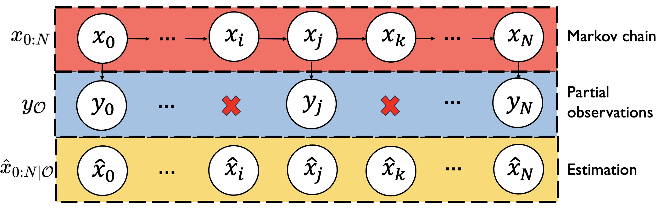
Figure 3: The estimation of state sequence under partial observations $y_{\mathcal{O}}$

Problem 3

$$\begin{array}[]{clll}\displaystyle\arg\min_{\hat{X}_{\mathcal{O}},K_{\mathcal{O}}}&J_{\mathcal{O}}=E[\|X-\hat{X}_{\mathcal{O}}\|^{2}]\\ \textrm{s.t.}&\hat{X}_{\mathcal{O}}=K_{\mathcal{O}}\cdot Y\\ \end{array}$$ (9)

where each element in $X$ and $Y$ satisfies

$$x_{t+1} \sim\mathcal{N}(Ax_{t},Q),\hskip 0.5ptt=0,\cdots,N,$$

$$y_{i} \sim\hskip 1.0pt\mathcal{N}(Cx_{i},R),\hskip 0.5pti\in\mathcal{O},$$

$$y_{j} \sim\hskip 1.0pt\mathcal{N}(0,\infty),\hskip 0.5ptj\notin\mathcal{O},$$

$$x_{0} \sim\hskip 1.0pt\mathcal{N}(0,P_{0}).$$

This problem is equivalent to finding the optimal estimation for each state individually. Based on the theory of linear estimation, the information from $y_{\mathcal{O}}$ can be well utilized by the Kalman filtering process and RTS smoother. The update of state estimation on the sequence follows this rule: deliver the past information forwards through prediction, fuse the sensor information through measurement update, and supplement future information backwards through the smoother. It is worth mentioning that for those states missing corresponding observations, we can skip the step of measurement update.

Lemma 1.

If the pair $(A,C)$ is observable, Problem 3 has a unique closed-form solution, which can be obtained through the following steps.

1. Calculate $\{K_{i}\}$,$\{F_{i}\}$ according to the Kalman filter and RTS smoother process. For those intermittent observations that $\{y_{j}|j\notin\mathcal{O}\}$, set the Kalman gain to zero $\{K_{j}=0|j\notin\mathcal{O}\}$.

2. Utilizing the $\{K_{i}\}$ and $\{F_{i}\}$ sequences, construct the $M_{\mathcal{O}}$, $L^{*}_{\mathcal{O}}$, and $H_{\mathcal{O}}$ matrices.

   $$M_{\mathcal{O}} =\begin{bmatrix}K_{0}&0&\cdots&0\\ \Phi(1)K_{0}&K_{1}&\cdots&0\\ \vdots&\vdots&\vdots&\vdots\\ \Phi(N)K_{0}&\Phi(N-1)K_{1}&\cdots&K_{N}\end{bmatrix},$$

   $$L^{*}_{\mathcal{O}} =\begin{bmatrix}I&0&\cdots&0\\ -CAK_{0}&I&\cdots&0\\ \vdots&\vdots&\vdots&\vdots\\ -C\Phi_{p}(N,1)K_{0}&-C\Phi_{p}(N,2)K_{1}&\cdots&I\end{bmatrix},$$

   $$H_{\mathcal{O}} =\begin{bmatrix}I-F_{0}\Phi(N)&\cdots&\cdots&F_{0}...F_{N-1}\\ \vdots&\vdots&\vdots&\vdots\\ 0&0&I-F_{N-1}\Phi(1)&F_{N-1}\\ 0&0&0&I\end{bmatrix},$$

   where $\Phi(k)=A^{k}$ and $\Phi_{p}(k,j)=\prod_{i=j}^{k-1}(A-AK_{i}C)$.

3. Calculate the solution of Problem 3.

   $$\hat{X}_{\mathcal{O}}=K_{\mathcal{O}}Y,~{}K_{\mathcal{O}}=H_{\mathcal{O}}M_{\mathcal{O}}L^{*}_{\mathcal{O}}$$

Remark 1.

In multi-sensor systems, we can also order observations chronologically, while allowing for any sequence of simultaneous measurements. The measurement update and time update processes of the Kalman filter are still valid, and the RTS smoother only needs to consider the final error covariance matrices and the state estimate at each time step.

The proof of Lemma 1 is in the appendix.A-A. Moreover, Lemma 1 provides the explicit linear relationship between estimated states $\hat{x}_{0:N|\mathcal{O}}$ and the observations $y_{\mathcal{O}}$. For those $\{y_{i}|i\notin\mathcal{O}\}$, when multiplied by the matrix $K_{\mathcal{O}}$, the corresponding weights are zeros, which clearly indicates that they are unrelated to the estimate.

IV-B Estimation update for the disordered new observation

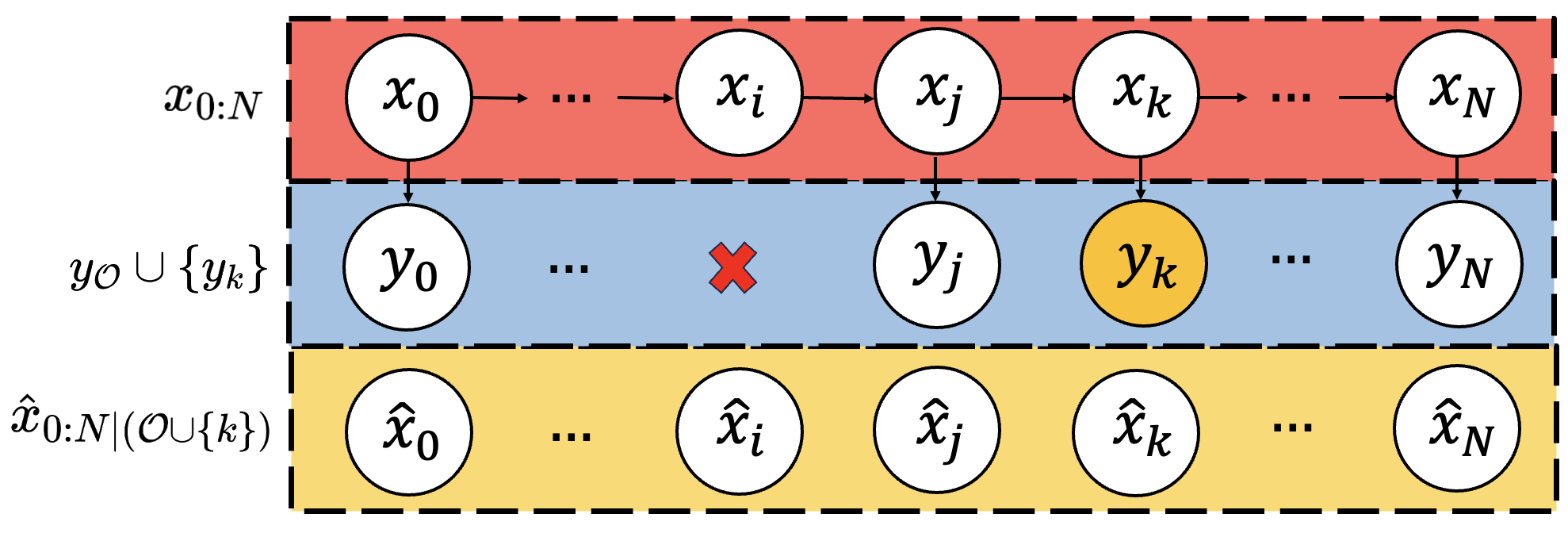
Figure 4: Estimation update for new observation $y_{k}$ under the previous observation set $y_{\mathcal{O}}$

Suppose that we have obtained the optimal estimation under $y_{\mathcal{O}}$. When a new observation $y_{k}$ is added to the observation set, the optimal estimation of state sequence should be updated with new observation set $y_{\mathcal{O}^{*}}=y_{\mathcal{O}}\cup\{y_{k}\}$. Here $y_{k}$ also follows the Gaussian distribution.

A basic approach is to use Lemma 1 to calculate the estimation of the state sequence under $y_{\mathcal{O}^{*}}$. In detail, we can utilize the known Kalman gain $\{K_{t}|t<k\}$ under $y_{\mathcal{O}}$ and recompute the rest process under $y_{\mathcal{O}^{*}}$, as illustrated in Fig. 5.

However, employing a direct method to compute the optimal estimate reveals imitations in computational cost. When $|y_{\mathcal{O}}|$ is large, especially in systems with multiple sensors, the direct method requires computing the matrix inverse $O(|y_{\mathcal{O}}|)$ times, which consumes significant computational resources. Furthermore, as the observation set expands, the optimal state estimate approaches the real state more closely. Nevertheless, adding new observations to a larger $y_{\mathcal{O}}$ requires an increasing number of calculation steps to update the estimate, especially in multi-sensor systems. This indicates that using direct method to update cannot fully leverage the information from the previous estimation, and thus causes a waste of computational resources.

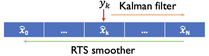
Figure 5: Recalculation steps for estimation update. When a new observation $y_{k}$ is inserted, the whole Kalman gain after time $k$ and the smoother gain for the entire sequence needs to be recalculated.

V Iterative approach for state estimation

In section IV, we discussed how to find the closed-form solution of equation (8), but its computational efficiency is poor. To speed up the solution and update process, we propose an iterative method for state sequence estimation that allows for rapid convergence to the optimal estimate.

The core idea of the iterative method is to fully utilize the previous estimates as the initial state in the iteration. By constructing a composite convex optimization problem, we design a proximal gradient descent algorithm to avoid redundant computations. Furthermore, we derive the convergence rate and the relationship between the iteration count and the reliability of estimates.

V-A The estimation of state sequence with partial observations

With the observation set $y_{\mathcal{O}}$, our objective is to optimize the function $\mathcal{L}_{\mathcal{O}}(\hat{x}_{0:N})$ in equation (8). The objective function incorporates two goals: first, the state estimates $\hat{x}_{0:N}$ should match the observations $\hat{y}_{\mathcal{O}}$; second, the state estimates $\hat{x}_{0:N}$ should conform to the known structure of the system. Therefore, $\mathcal{L}_{\mathcal{O}}$ can be considered as the sum of two functions:

$$f =\sum_{i\in\mathcal{O}}\|y_{i}-C\hat{x}_{i}\|^{2}_{R^{-1}}$$ (10)

$$g =\|\hat{x}_{0}\|^{2}_{P_{0}^{-1}}+\sum_{i=1}^{N}\|\hat{x}_{i}-A\hat{x}_{i-1}\|^{2}_{Q^{-1}}$$ (11)

We can represent each $\hat{x}_{i}$ using a column vector $\hat{X}=col\{\hat{x}_{0|\mathcal{O}},\cdots,\hat{x}_{N|\mathcal{O}}\}$. Next, we can construct a sparse matrix $\tilde{\mathcal{A}}$, which captures the relationship between the states:

$$\begin{bmatrix}\hat{x}_{0}\\ \hat{x}_{1}-A\hat{x}_{0}\\ \hat{x}_{2}-A\hat{x}_{1}\\ \vdots\\ \hat{x}_{N}-A\hat{x}_{N-1}\end{bmatrix}=\begin{bmatrix}I&0&0&\cdots&0\\ -A&I&0&\cdots&0\\ 0&-A&I&\cdots&0\\ \vdots&\vdots&\vdots&\ddots&\vdots\\ 0&0&0&\cdots&I\end{bmatrix}\begin{bmatrix}\hat{x}_{0}\\ \hat{x}_{1}\\ \hat{x}_{2}\\ \vdots\\ \hat{x}_{N}\end{bmatrix}=\tilde{\mathcal{A}}\hat{X}.$$ (12)

Thus the function $g$ can be written in the quadratic form:

$$g(\hat{X})=\|\tilde{\mathcal{A}}\hat{X}\|_{\tilde{P}^{-1}}^{2}=\|\hat{X}\|^{2}_{\tilde{\mathcal{A}}^{T}\tilde{P}^{-1}\tilde{\mathcal{A}}}$$ (13)

where $\tilde{P}$ is a block-diagonal matrix,

$$\tilde{P}=\begin{bmatrix}P_{0}&0&0&\cdots&0\\ 0&Q&0&\cdots&0\\ 0&0&Q&\cdots&0\\ \vdots&\vdots&\vdots&\ddots&\vdots\\ 0&0&0&\cdots&Q\end{bmatrix}.$$

With the help of equation (13), we convert Problem 2 to a composite convex optimization problem.

Problem 4

$$\begin{array}[]{clll}\displaystyle\arg\min_{\hat{X}}&~{}\mathcal{L}_{\mathcal{O}}=f_{\mathcal{O}}(\hat{X})+g(\hat{X})\end{array}$$ (15)

where

$$f_{\mathcal{O}}(\hat{X}) =\sum_{i\in\mathcal{O}}\|y_{i}-\tilde{C}_{i}\hat{X}\|^{2}_{R^{-1}},$$

$$g(\hat{X}) =\|\hat{X}\|_{H}^{2},\quad H={\tilde{\mathcal{A}}^{T}\tilde{P}^{-1}\tilde{\mathcal{A}}},$$

and $\tilde{C}_{i}$ is a row block matrix, with the i-th block being matrix $C$, while all other blocks are zero matrices.

The term $f_{\mathcal{O}}(\hat{X})$ represents the goal of fitting the observation information, which evolves as the observation set is updated. The term $g(\hat{X})$ represents a kind of normalization of estimated states, aiming to conform the system structure.

Remark 2.

If the function $h(x)$ is an $L$-smooth and $\lambda$-strongly convex function, it satisfies the following condition: $\forall x,x^{0}$,

$$h(x) \leq h(x^{0})+\nabla h(x^{0})^{T}(x-x^{0})+\frac{L}{2}\|x-x^{0}\|^{2}_{2},$$

$$h(x) \geq h(x^{0})+\nabla h(x^{0})^{T}(x-x^{0})+\frac{\lambda}{2}\|x-x^{0}\|^{2}_{2}.$$

Proposition 1.

Suppose the smooth and strong convexity of $f_{\mathcal{O}}(\hat{X})$ and $g(\hat{X})$ holds with $L_{f},\lambda_{f},L_{g},\lambda_{g}$, then the following inequalities hold

$$L_{f} =\begin{cases}0,&\text{if }\mathcal{O}=\emptyset\\ \lambda_{\text{max}}(C^{T}R^{-1}C),&\text{otherwise}\end{cases},$$

$$\lambda_{f} =\begin{cases}\lambda_{\text{min}}(C^{T}R^{-1}C),&\text{if }\mathcal{O}=\{0,1,2,\dots,N\}\\ 0,&\text{otherwise}\end{cases},$$

$$L_{g} =\lambda_{max}(H)\geq\lambda_{min}(H)=\lambda_{g}\geq 0.$$

Therefore, we can use proximal gradient descent to find the optimal solution iteratively. Define the function $f^{t}_{\mathcal{O}}(x)$ as the approximate function, and $prox_{\eta g}(\cdot)$ as the proximal operator:

$$f^{t}_{\mathcal{O}}(x)=f(x^{t})+\nabla f_{\mathcal{O}}(x^{t})^{T}(x-x^{t})+\frac{1}{2\eta_{t}}\|x-x^{t}\|^{2}_{2},$$ (16)

$$prox_{\eta g}(x)=\arg\min_{z}\left[\frac{1}{2}\|z-x\|^{2}_{2}+\eta g(z)\right].$$ (17)

Theorem 2 demonstrates how to iteratively solve for the optimal solution to Problem 4. The proof can be found in Appendix A-B.

Theorem 2.

Suppose $X^{*}$ is the unique solution of Problem 4. With the fixed learning rate $\eta=\frac{1}{\lambda_{\text{max}}(C^{T}R^{-1}C)}\leq\frac{1}{L_{f}}$, repeat the following step and $X^{t}$ will converge to $X^{*}$.

$$X^{t+1} =prox_{\eta g}(\arg\min_{X}f^{t}_{\mathcal{O}}(X))$$

$$=prox_{\eta g}(X^{t}-\eta\nabla f_{\mathcal{O}}(X^{t}))$$

$$=(I+\eta H)^{-1}(X^{t}-\eta\nabla f_{\mathcal{O}}(X^{t}))$$ (18)

Then one has the following result (convergence rate):

$$\mathcal{L}_{\mathcal{O}}(X^{t})\leq\mathcal{L}_{\mathcal{O}}(X^{*})+(1-\theta)^{t}[\mathcal{L}_{\mathcal{O}}(X^{0})-\mathcal{L}_{\mathcal{O}}(X^{*})]$$ (19)

where $\theta=(\eta\lambda_{f}+\eta\lambda_{g})/(1+\eta\lambda_{g})$.

Remark 3.

In multi-sensor systems, the only difference is the function $f_{\mathcal{O}}$, which is composed of observations from multiple different sensors. The iterative update process and the derivation of the convergence rate are similar to those in a single-sensor system.

We can interpret this iterative process from the perspective of Kalman filter and RTS smoother. The term $X^{t}-\eta\nabla f_{\mathcal{O}}(X^{t})$ is comparable to the measurement update step in Kalman filtering, where $\nabla f_{\mathcal{O}}(X^{t})$ corresponds to the residual and a fixed parameter $\eta$ corresponds to the Kalman gain. The term $(I+\eta H)^{-1}$ plays the role of a smoother, updating the estimate based on the system structure.

Solving Problem 4 using Theorem 2 will yield the same result as solving Problem 3 with Lemma 1. However, compared to Lemma 1, the iterative approach provides by Theorem 2 does not require calculating the Kalman gain and smoother gain at each step. Instead, it replaces the Kalman gain with a fixed parameter $\eta$ and the smoother gain with a fixed matrix $(I+\eta H)^{-1}$, converging to the optimal estimate after several iterations. This provides a new perspective on estimation update.

V-B Estimation update for the disordered new observation

Suppose that we have computed the optimal estimate $\hat{X}_{\mathcal{O}}$ under $y_{\mathcal{O}}$. Then, as shown in Fig. 4, a new observation $y_{k}$ is added to the observation set, and we attempt to update the state sequence estimate using Theorem 2.

Denote the updated observation set as $y_{\mathcal{O^{*}}}=y_{\mathcal{O}}\cup\{y_{k}\}$. Algorithm 1 provides the details of calculating the optimal estimate with iterative method.

Input: the system parameters $\{A,C,Q,R\}$ and the stop condition $\epsilon$

Input: initial state $(\bar{x}_{0}=0,\bar{P}_{0})$ and the full observation set $y_{0:N}$

Output: estimation of state sequence $\{\hat{x}_{0},\cdots,\hat{x}_{N}\}$

1 Calculate the matrix $H,L_{f}$ and $R^{-1}$;

2 Choose the $\eta<1/L_{f}$ and calculate $(I+\eta H)^{-1}$;

3 Initialize $\mathcal{O}=\emptyset$, $\hat{X}_{\mathcal{O}}=col\{\hat{x}_{0|\mathcal{O}}=0,\cdots,\hat{x}_{N|\mathcal{O}}=0\}$;

// update with new observations

4 repeat

5       if $\mathcal{O}$ changes to $\mathcal{O}^{*}$ then

6             $\hat{X}=\hat{X}_{\mathcal{O}}$;

7             repeat

8                   $\nabla f_{\mathcal{O}^{*}}=\sum_{i\in\mathcal{O}^{*}}C_{i}^{T}R^{-1}(y_{i}-C_{i}\hat{X})$;

9                   $\hat{X}^{*}=(I+\eta H)^{-1}(\hat{X}-\eta\nabla f_{\mathcal{O}^{*}}(\hat{X}))$;

10                   if $|\mathcal{L}_{\mathcal{O}^{*}}(\hat{X})-\mathcal{L}_{\mathcal{O}^{*}}(\hat{X}^{*})|<\epsilon$ then

11                         break;

12                        

13                  else

14                         $\hat{X}=\hat{X}^{*}$;

15                        

16                  

17            until ;

18            $\mathcal{O}=\mathcal{O}^{*},\hat{X}_{\mathcal{O}}=\hat{X}^{*}$;

19            

20      

21until ;

Algorithm 1 Iterative approach for state estimation

Compared to the direct approach, this iterative method for updating estimates has two advantages. Firstly, the iterative method does not compute the inverse matrix to obtain the optimal gain, but only requires matrix multiplication, and the fixed inverse matrices $(I+\eta H)^{-1}$ and $R^{-1}$ can be calculated in advance. Secondly, the previous estimate can be used as the initial value of the iteration, and the information in the previous observation set can be fully utilized.

When $|y_{\mathcal{O}}|$ is large, the term $f_{\mathcal{O}}$ has slightly change with new observations, leading to minor differences between $\hat{X}_{\mathcal{O}^{*}}$ and $\hat{X}_{\mathcal{O}}$. This implies that, as the impact of the new observation on $f_{\mathcal{O}}$ becomes more negligible, the algorithm will converge more rapidly. Theorem 3 provides a quantitative analysis of the maximum number of iterations when new observations are added. The proof can be found in Appendix A-C.

Theorem 3.

Suppose that the observation set changes from $y_{\mathcal{O}}$ to $y_{\mathcal{O^{*}}}=y_{\mathcal{O}}\cup\{y_{k}\}$. Let the $X^{0}=\hat{X}_{\mathcal{O}}$ as the initial value of the iterations and $x_{k}\sim\mathcal{N}(\hat{x}_{k|\mathcal{O}},P_{k|\mathcal{O}})$. If the optimal solution is $X^{*}$ and the stop condition is $\epsilon$ that $|L_{\mathcal{O^{*}}}(X^{\tau})-L_{\mathcal{O^{*}}}(X^{*})|<\epsilon$, the maximum iteration number $\tau$ satisfies

$$\tau<\log_{1-\theta}\left({\frac{\epsilon}{\|\Xi\xi\|^{2}_{R^{-1}}+2\|\Xi\|_{R^{-1}}\|\xi\|_{R^{-1}}}}\right)$$ (20)

where

$$\xi =y_{k}-C\hat{x}_{k|\mathcal{O}},$$

$$\Xi =CP_{k|\mathcal{O}}C^{T}(CP_{k|\mathcal{O}}C^{T}+R)^{-1}.$$

Theorem 3 demonstrates that the more reliable the initial $\hat{x}_{k}$ is, the fewer iterations are required for convergence. Thus, as the observation set $y_{\mathcal{O}}$ expands, the number of iterations required for the estimation update decreases.

VI Algorithm and analysis

In this section, we aim to solve the targeted MIP problem presented in (7). Summarized in Fig. 6, the GBS estimator involves repeating two steps: assessing the reliability of observations and updating estimates. The algorithms introduced in Section IV and Section V facilitate the estimation update in response to changes in reliable observation set.

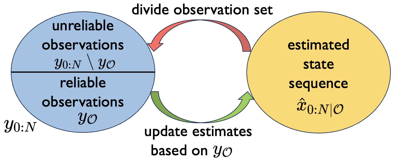
Figure 6: The framework of GBS estimator. GBS estimator comprises two components: the resilient estimator and the secure detector. The green arrow indicates the resilient estimator, which estimates the state based on reliable observations. The red arrow denotes the secure detector, which identifies reliable observations based on the estimated state.

VI-A Initial strategy for rough estimation

A good initial value is beneficial in solving problems. However, at the beginning, we do not know the initial values of $\hat{p}_{0:N}$ and $\hat{x}_{0:N}$. Therefore, the initial strategy is targeted to roughly estimate the value of observation indicators $p_{0:N}$ based on $y_{0:N}$.

The key idea of the initial strategy is to estimate $\{\hat{x}_{t}\}$ sequentially and to roughly determine the value of $\hat{p}_{t+1}$ through $\hat{x}_{t}$. If $\hat{p}_{t+1}=0$, the observation $y_{t+1}$ is utilized for the state estimation of $x_{t+1}$ through Kalman filter. Algorithm 2 provides the details of initial strategy.

Input: the system parameters $\{A,C,Q,R,\alpha\}$

Input: the initial state estimate $(\bar{x}_{0}=0,\bar{P}_{0})$ and the full observation set $y_{0:N}$

Output: estimated indicators $\hat{p}_{0:N}$ and state $\hat{x}_{0:N}$

1 Initial $\hat{x}_{0}=\bar{x}_{0},P_{0}=\bar{P}_{0}$;

2 for $i=0$ to $N$ do

       // determine the indicators

3       $\hat{p}_{i}=\textbf{bool}(\|y_{i}-C\hat{x}_{i}\|^{2}_{R^{-1}}<\alpha)$;

       // estimate the state

4       if $p_{i}=1$ then

5             $K_{i}=P_{i}C^{T}(CP_{i}C^{T}+R)^{-1}$;

6             $\hat{x}_{i}=\hat{x}_{i}+K_{i}(y_{i}-C\hat{x}_{i})$;

7             $P_{i}=(I-K_{i}C)P_{i}$;

8            

9       $\hat{x}_{i+1}=A\hat{x}_{i}$;

10       $P_{i+1}=AP_{i}A^{T}+Q$;

11      

Algorithm 2 Initial strategy for rough estimation

VI-B Gaussian-Bernoulli Secure (GBS) estimator

The approach to solving Problem 1 is to iteratively seek the optimal estimate by fixing the $\hat{p}_{0:N}$ and $\hat{x}_{0:N}$, respectively.

First, consider to minimize the objective function with fixed $\hat{p}_{0:N}^{*}$. When $\hat{p}_{i}^{*}=0$, the term $(1-\hat{p}_{i}^{*})\|y_{i}-C\hat{x}_{i}\|^{2}_{R^{-1}}$ is active, meaning that the objective will consider the “fit” between the state and the measurement. When $\hat{p}_{i}^{*}=1$, the term $(1-\hat{p}_{i}^{*})\|y_{i}-C\hat{x}_{i}\|^{2}_{R^{-1}}$ is non-functional, meaning to reject using such observation information to “update” the state estimation. Thus, we can simplify equation (7) as follows:

$$\arg\min_{\hat{x}_{0:N}}~{}\mathcal{W}(\hat{x}_{0:N},\hat{p}_{0:N}^{*})=\mathcal{L}_{\mathcal{O}}(\hat{x}_{0:N}),$$ (21)

where the set $\mathcal{O}=\{i,|\hat{p}_{i}^{*}=0\}$. For LMMSE estimator and MAP estimator achieve the same result, we can implement either the direct approach (Lemma 1) or the iterative approach (Theorem 2) to calculate optimal $\hat{x}_{0:N}$.

Second, seek the minimal $\hat{p}_{0:N}$ with fixed state estimation $\hat{x}_{0:N}^{*}$. When state estimation $\hat{x}_{i}^{*}$ is determined, the term $(1-\hat{p}_{i})\|y_{i}-C\hat{x}_{i}^{*}\|^{2}_{R^{-1}}$ is debatable, depending on the comparison between $\|y_{i}-C\hat{x}_{i}^{*}\|^{2}_{R^{-1}}$ and the penalty $\alpha$. Equation (7) with fixed $\hat{x}_{0:N}^{*}$ can be written as follows:

$$\arg\min_{\hat{p}_{0:N}}~{}\mathcal{W}(\hat{x}_{0:N}^{*},\hat{p}_{0:N})$$

$$= \biggl{\{}\sum_{i=0}^{N}[(1-\hat{p}_{i})\|y_{i}-C\hat{x}_{i}^{*}\|^{2}_{R^{-1}}+\hat{p}_{i}\alpha]\biggr{\}}$$ (22)

and its solution can be easily obtained

$$\hat{p}_{i}=\textbf{bool}(\|y_{i}-C\hat{x}_{i}^{*}\|^{2}_{R^{-1}}>\alpha).$$ (23)

However, the aforementioned iteration may be rigid and often converges to suboptimal points. Here, we consider optimizing the indicator $\hat{p}_{k}$ simultaneously with the estimated states $\hat{x}_{0,N}$. Denote the index set as $\mathcal{O}_{k}^{+}=\{i|\hat{p}^{*}_{i}=0\}\cup\{k\}$ and $\mathcal{O}_{k}^{-}=\mathcal{O}_{k}^{+}\setminus\{k\}$. Then, the portion of the objective function in (7) that includes $\hat{p}_{k}$ and $\hat{x}_{0:N}$ can be written as two parts:

$$\mathcal{L}_{\mathcal{O}_{k}^{-}}(\hat{x}_{0:N})= \Biggl{\{}\sum_{i\in\mathcal{O}_{k}^{-}}\|y_{i}-C\hat{x}_{i}\|^{2}_{R^{-1}}+\|\hat{x}_{0}\|^{2}_{P_{0}^{-1}}$$

$$+\sum_{i=1}^{N}\|\hat{x}_{i}-A\hat{x}_{i-1}\|^{2}_{Q^{-1}}\Biggr{\}},$$ (24)

$$\mathcal{P}_{k}(\hat{p}_{k})= (1-\hat{p}_{k})\|y_{k}-C\hat{x}_{k}\|^{2}_{R^{-1}}+\hat{p}_{k}\alpha.$$ (25)

We can update $\hat{p}_{k}$ by solving the following optimization problem:

$$\begin{array}[]{clll}\displaystyle\arg\min_{\hat{p}_{k},\hat{x}_{0:N}}&\biggl{\{}\mathcal{L}_{\mathcal{O}_{k}^{-}}(\hat{x}_{0:N})+\mathcal{P}_{k}(\hat{p}_{k})\biggl{\}}\end{array}$$ (26)

and the optimal $\hat{p}_{k}$ can be determined by:

$$\hat{p}_{k}=\textbf{bool}((\min\mathcal{L}_{\mathcal{O}_{k}^{+}}-\min\mathcal{L}_{\mathcal{O}_{k}^{-}})>\alpha).$$ (27)

As described in Algorithm 3, we iteratively calculate equation (21) and (VI-B), and improve the optimality through equation (26).

Input: the system parameters $\{A,C,Q,R,\alpha,\tau\}$

Input: the initial state estimate $(\bar{x}_{0},\bar{P}_{0})$ and the full observation set $y_{0:N}$

Output: $\hat{x}_{0:N},\hat{p}_{0:N}$

1 Initialize $\hat{x}_{0:N}^{0},\hat{p}_{0:N}^{0}$ using Algorithm 2 ;

2 Set the count $k=0$ and ${\mathcal{O}^{0}}=\{i|\hat{p}_{i}^{0}=0\}$;

3 repeat

4       $k\leftarrow k+1$;

       // $\arg\min_{\hat{p}_{0:N}}~{}\mathcal{L}(\hat{x}_{0:N}^{*},\hat{p}_{0:N})$

5       for $i=0$ to $N$  do

6             $\hat{p}_{i}^{k}=\textbf{bool}(\|y_{i}-C\hat{x}_{i}^{*}\|^{2}_{R^{-1}}>\alpha)$;

7            

8      update $\mathcal{O}^{k}=\{i|\hat{p}_{i}^{k}=0\}$;

       // check suboptimal points

9       if $\mathcal{O}^{k}=\mathcal{O}^{k-1}$ then

10             for $i=0$ to $N$ do

11                   $\hat{p}_{i}^{*}=\textbf{bool}((\min\mathcal{L}_{\mathcal{O}_{i}^{+}}-\min\mathcal{L}_{\mathcal{O}_{i}^{-}})>\alpha)$;

12                   if $\hat{p}_{i}^{*}\neq\hat{p}_{i}^{k}$ then

13                         $\hat{p}_{i}^{k}=\neg\hat{p}_{i}^{k}$ and update $\mathcal{O}^{k}$ ;

14                         break;

15                        

16                  

17            

      // $\arg\min_{\hat{x}_{0:N}}~{}\mathcal{L}(\hat{x}_{0:N},\hat{p}_{0:N}^{*})$

18       if $\mathcal{O}^{k}=\mathcal{O}^{k-1}$ then

19             break;

20            

21      else

22             update optimal estimates $\hat{x}_{0:N}$;

23            

24      

25until ;

// judge status of observations

26 if $|\mathcal{O}^{k}|<(N+1-\tau)$ then

27       Print: info(”attack alarm in this sensor!”);

28      

Algorithm 3 Gaussian-Bernoulli Secure Estimator

VI-C Convergence analysis

Here, we prove the convergence of our GBS estimator algorithm.

First, we demonstrate the existence of the solution to our target MIP problem presented in (7). As a $0-1$ sequence $\hat{p}_{0:N}\in\{0,1\}^{(N+1)}$, there are a total of $2^{(N+1)}$ cases. For $\{0,1\}^{(N+1)}\leftrightarrow 2^{\{0,\cdots,N\}}$, we can define a mapping from the indicator set to the index set that

$$\mathcal{O}^{*}=\mathcal{G}(\hat{p}_{0:N}^{*})=\{i|\hat{p}^{*}_{i}=0\}$$ (28)

When the observation set is fixed, the optimal estimation can be obtained as a unique solution through Lemma 1 or Theorem 2. We can also define it as a mapping:

$$\hat{x}_{0:N}^{*}=\mathcal{H}(\mathcal{O}^{*})=\arg\min_{\hat{x}_{0:N}}\mathcal{L}_{\mathcal{O}^{*}}(\hat{x}_{0:N})$$ (29)

Therefore, the optimal solution of the Problem 1 can be found through finite enumeration.

$$\arg\min_{\hat{p}^{*}}\hskip 8.5359pt\mathcal{W}((\mathcal{H}\circ\mathcal{G})(\hat{p}^{*}),\hat{p}^{*}),~{}\hat{p}^{*}\in\{0,1\}^{(N+1)}$$ (30)

Then, we prove that $\hat{p}^{k}$ will ultimately converge, thereby determining $\hat{x}_{0:N}$. Assume that at the $k-$th iteration, $\hat{x}_{0:N}^{k}=(\mathcal{H}\circ\mathcal{G})(\hat{p}^{k}_{0:N})$. When updating the $\hat{p}^{k+1}_{0:N}$ and $\hat{x}^{k+1}_{0:N}$ according to Algorithm 3, the following inequality holds:

$$\mathcal{W}(\hat{x}_{0:N}^{k+1},\hat{p}^{k+1}_{0:N})\leq\mathcal{W}~{}(\hat{x}_{0:N}^{k},\hat{p}^{k+1}_{0:N})\leq\mathcal{W}(\hat{x}_{0:N}^{k},\hat{p}^{k}_{0:N}).$$ (31)

Therefore, the $0-1$ sequence $\hat{p}_{0:N}$ will iteratively minimize the objective function $\mathcal{W}$ in a monotonically nonincreasing way until $\hat{p}^{k+1}_{0:N}=\hat{p}^{k}_{0:N}$.

VII experiment

In this section, we introduce the comprehensive experimental results. First, we compare the update speeds of direct and iterative methods under different observation update rules. Then, We compare our GBSE with other detectors and estimators from the perspectives of detection rate of attacks and error in state estimation. Next, we demonstrate the detection capabilities of our GBSE algorithm in a multi-sensor system subjected to multiple attacks. The code is available at GitHub: https://github.com/RoboCubPilot/GB_secure_estimator.git.

Although our previous focus is on the single-sensor system, the derivation process and conclusions are also applicable to multi-sensor systems. For a multi-sensor system equipped with $M$ sensors, $y_{i,j}$ denotes the observation at sensor $j$ at time $i$, and the corresponding indicator is defined as $p_{i,j}$.

VII-A Comparison of direct approach and iterative approach

Consider a 3-dimensional system with $M$ sensors over the interval $T=[0,N]$:

$$M=N=100,\hskip 5.69046ptx_{0}\sim\mathcal{N}(0,I),\hskip 5.69046ptA=C=I,$$

$$Q_{i}=R_{j}=\begin{bmatrix}1&0.5&0\\ 0.5&1&0.5\\ 0&0.5&1\end{bmatrix},\begin{matrix}i=0,...,N\\ j=1,...,M\end{matrix}.$$

The full observation set is $y_{0:N,1:M}$. The observation set is updated according to a specific pattern, denoted as $\mathcal{O}_{k}\in 2^{\{0,\cdots,N\}\otimes\{1,\cdots,M\}}$ for the $k-$th update. Our algorithm is to update the state estimates of $x_{0:N}$ based on the observation set $\mathcal{O}_{k}$.

First, in Fig. 7(a), we implement experiments to add observations along the timeline, which is the default observation update rule for most systems. The newly added observations include the observations from all sensors at time $k$ that $\mathcal{O}_{k}\setminus\mathcal{O}_{k-1}=\{k\}\otimes\{1,\cdots,M\}$. Additionally, in Fig. 7(b), we are interested in incorporating observations in the order of sensor indices. The rules for observation updates allow the system to update one after another based on the reliability of the sensors. The new observations add to the set from $k$-th sensor that $\mathcal{O}_{k}\setminus\mathcal{O}_{k-1}=\{0,\cdots,N\}\otimes\{k\}$. Moreover, in Fig. 7(c), we test randomly updated observation sets. In Algorithm 4, the update rule is unpredictable, simulating random observation masking. After masking part of the full set, we calculate the optimal estimate, then reintroduce masked observations, recording estimation times.

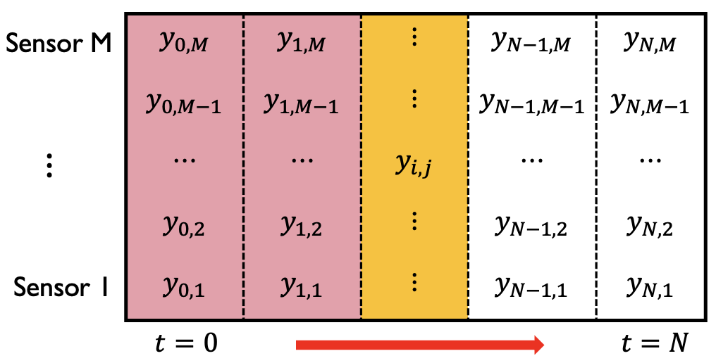
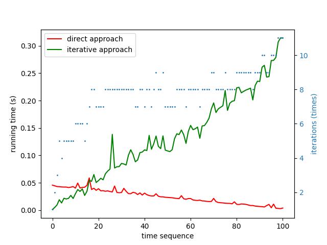
(a) add observations along the timeline

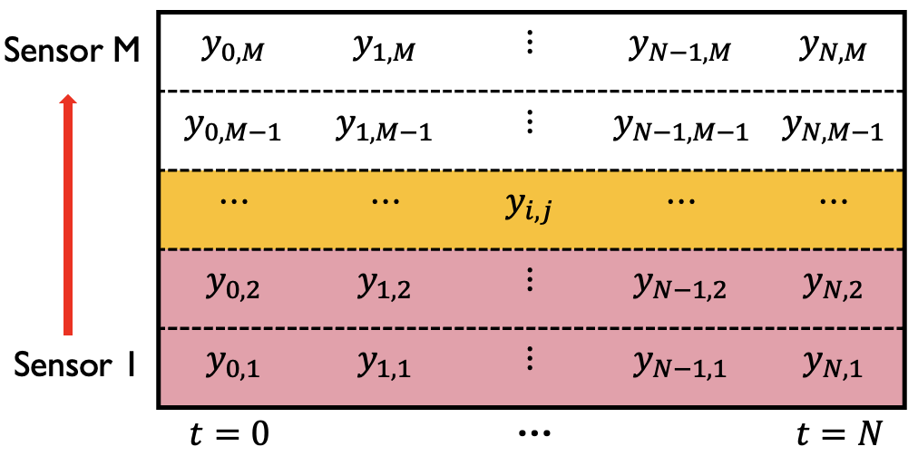
(b) add observations in the order of sensor indices

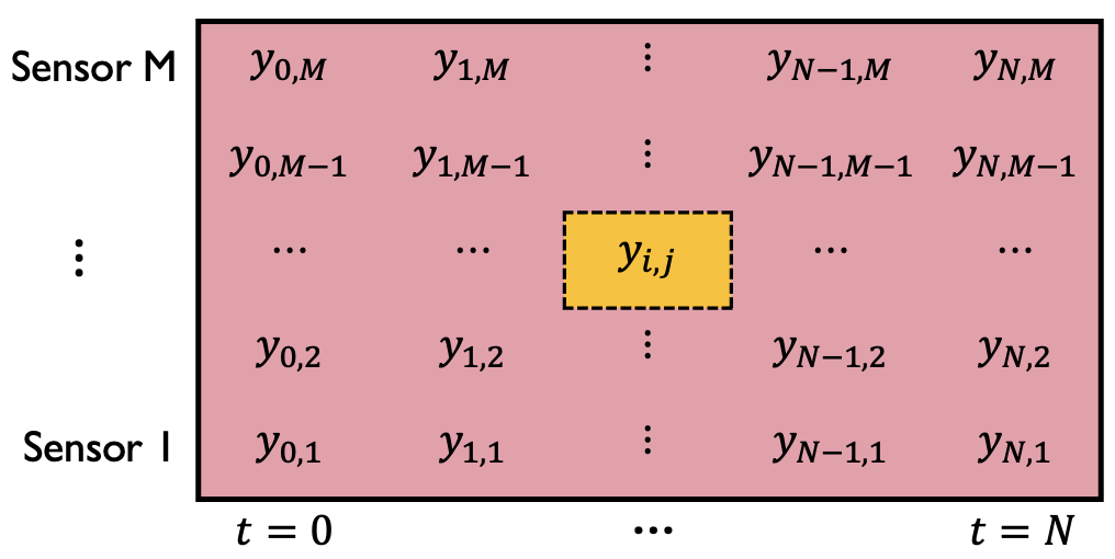
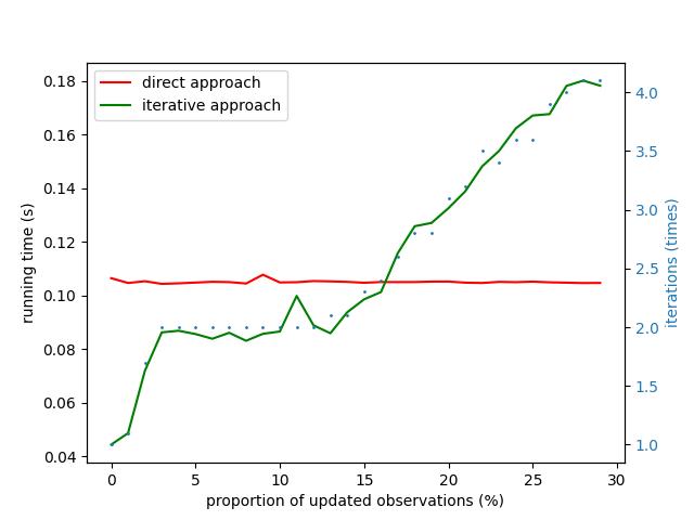
(c) insert the different proportions of observations

Figure 7: Comparison of direct approach and iterative approach under different observation update rules. In the left figure, the arrow indicates the direction of the observation updates, with the pink representing the past observation set and the yellow representing the newly added observations. In the right figure, the blue dots represent the number of iterations of the iterative approach.

The results show that the direct and iterative methods work best in different situations. The direct method is more efficient for timeline-based updates, while the iterative method is better when only a small, unordered part of the observation set is updated. The iterative method is also preferred when adding new sensor data to the observation set.

VII-B Compared with other detector and estimator

Consider the scale system with two sensors at interval $T=[0,N]$, where $x_{0}\sim\mathcal{N}(0,1),A=1,C_{1}=C_{2}=1,Q=0.5,R_{1}=R_{2}=2,N=20$. Let’s consider that sensor $1$ is functioning normally, while sensor $2$ has been injected with false information under attack at time $t$. Therefore,

$$\tilde{y}_{t,2}=y_{t,2}+e_{t},\>t=1,2,..,20,$$ (32)

where $e_{t}$ denotes the injected attack signal.

First, we implement the three common attack strategies in our experiment. Fig. 8(a) represents the application of random interference, where $e_{t}\sim N(0,\tilde{R})$. Fig. 8(b) indicates a constant effect on the sensor, where $e_{t}=\mu_{\text{constant}}$ starting from time $t=10$. Fig. 8(c) illustrates a uniformly increasing impact on the sensor, where $e_{t}=\frac{t}{N}\mu_{\text{max}}$.

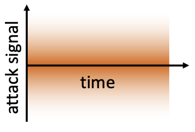
(a) random inference

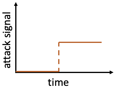
(b) constant bias

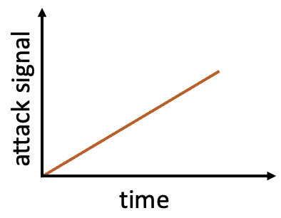
(c) increasing bias

Figure 8: Illustration of three types of attacks in our experiment

Then, we introduce the other detectors and estimators that our algorithm is compared against.

VII-B1 $\chi^{2}$ detector

The idea is to calculate the probability of the Kalman residuals and compare it with $\alpha_{\text{threshold}}$.

$$\chi^{2}_{t}=\|y_{t}-C\hat{x}_{t|t-1}\|^{2}_{\sum_{r_{t}}^{-1}}\ \underset{}{\overset{}{\gtrless}}\ \alpha_{\text{threshold}}.$$ (33)

VII-B2 CUSUM detector

It calculates the cumulative sum of the differences between the Kalman residuals and a reference $\delta_{\text{ref}}$ in different direction.

$$S_{t}=\max(0,S_{t-1}+(r_{t}-\delta_{\text{ref}}))\ \underset{}{\overset{}{\gtrless}}\ \alpha_{\text{threshold}},$$ (34)

where we set the $\delta_{\text{ref}}=0.5$.

VII-B3 Resilient estimator

The resilient estimator determines attacks by comparing $\chi^{2}$ with $\alpha_{\text{threshold}}$, but directly ignores those observations that exceed the $\alpha_{\text{threshold}}$.

VII-B4 Gaussian-Bernoulli Secure (GBS) estimator

Our proposed GBS estimator in Algorithm. 3 also needs to set the parameter $\alpha_{\text{threshold}}$ to determine low-probability events and the parameter $\tau_{\text{tolerant}}$ to tolerate their occasional occurrence.

We choose $\alpha_{\text{threshold}}=6$ and $\tau_{\text{tolerant}}=3$ that allows the detector and estimator to achieve optimal performance. We test their performance with varying attack intensities. The intensity is a topic of greater concern for us because, there is a trade-off between their stealthiness and the impact on state estimation. As shown in Fig. 9, we select six different levels of intensity for each type of attacks, ranging from mild to severe. For each attack intensity, we randomly simulate 10,000 observation sequences under attack.

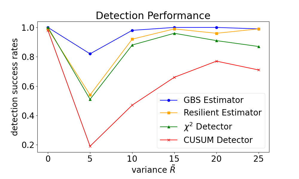
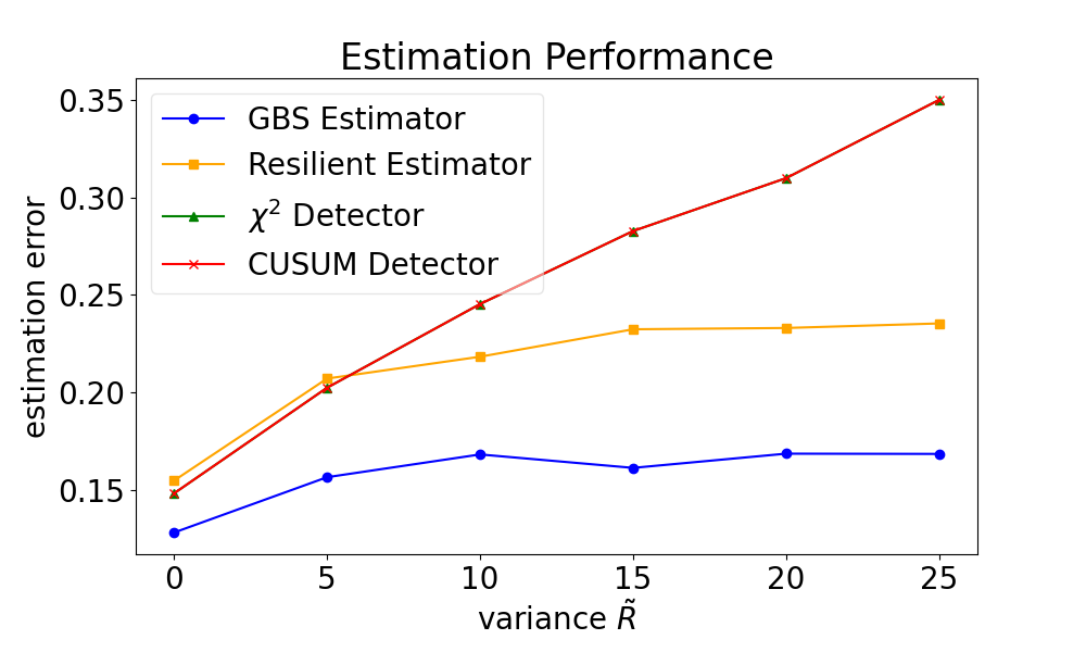
(a) random interference attack with different intensity

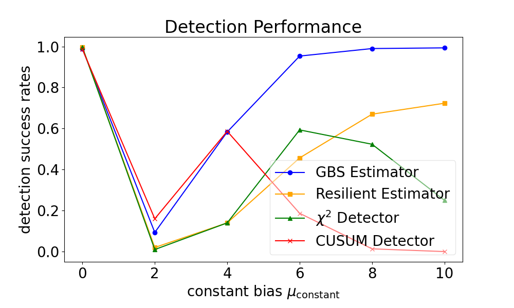
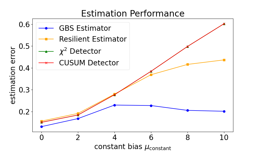
(b) constant bias attack with different intensity

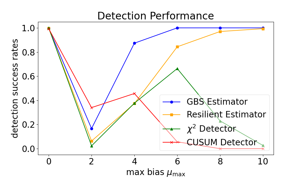
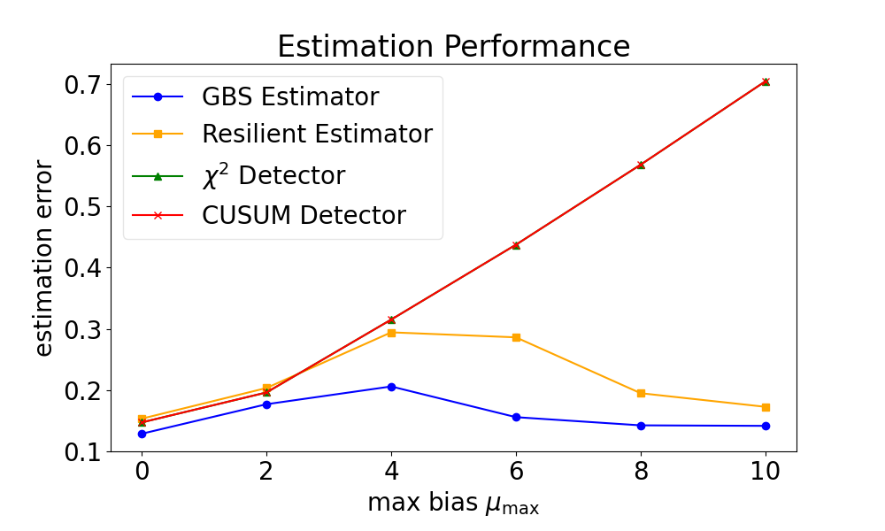
(c) uniformly increasing bias attack with different intensity

Figure 9: Comparison of GSB Estimator’s performance with other algorithms under different types of attacks and varying intensities. In the left figure, we compare the detection success rate with other algorithms. In the right figure, we compare the estimation error with other algorithms.

The results demonstrate that the detection success rate of the GBS estimator increases with the intensity of the attacks, which is intuitive. The estimation error of the GBS estimator does not continuously increase with the attack intensity; instead, it initially rises slightly and then stabilizes. Compared to other detectors and sensors, the GBS estimator generally performs better in both detection and estimation.

We further provide the detection success rate and estimation accuracy for different values of parameters $\alpha_{\text{threshold}}$ and $\tau_{\text{tolerant}}$ in Appendix B-B. The results show that the GBS estimator consistently outperforms other algorithms, regardless of the parameter choices.

VII-C Multiple attacks in multi-sensor system

In a multi-sensor system, as the number of sensors under attack increases, how to maintain the resilient state estimation and detect the attacked sensors is challenging. The reason is that, with the increase number of observations, attacks are more easily concealed among outliers, which are those occasional observations with significant errors.

Consider a scalar system with $M=20$ sensors at interval $T=[0,20]$, where $x_{0}\sim\mathcal{N}(0,1),A=1,Q=0.5.$ All sensors are supposed to satisfy following observation model. For each $i\in T$,

$$y_{i,j}\sim\mathcal{N}(x_{i},R_{j}=20),\hskip 8.5359ptj=1,\cdots,20.$$

Suppose we deploy noise interference on sensors indexed from $1$ to $5$. When these attacks last from $i=0$ to $20$, the actual observation model becomes:

$$y_{i,j}\sim\mathcal{N}(x_{i},\tilde{R}_{j}=100),j=1,\cdots,5.$$

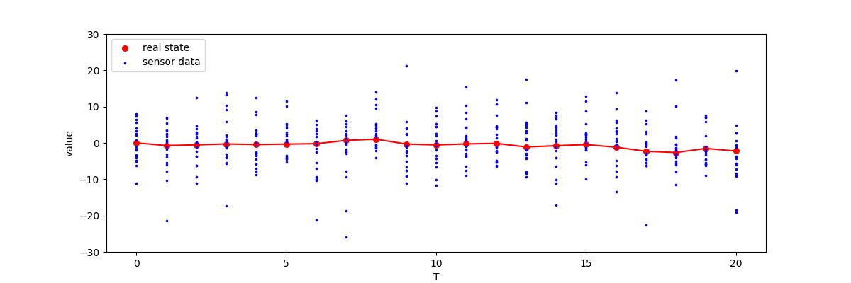
(a) system state and multiple sensor data

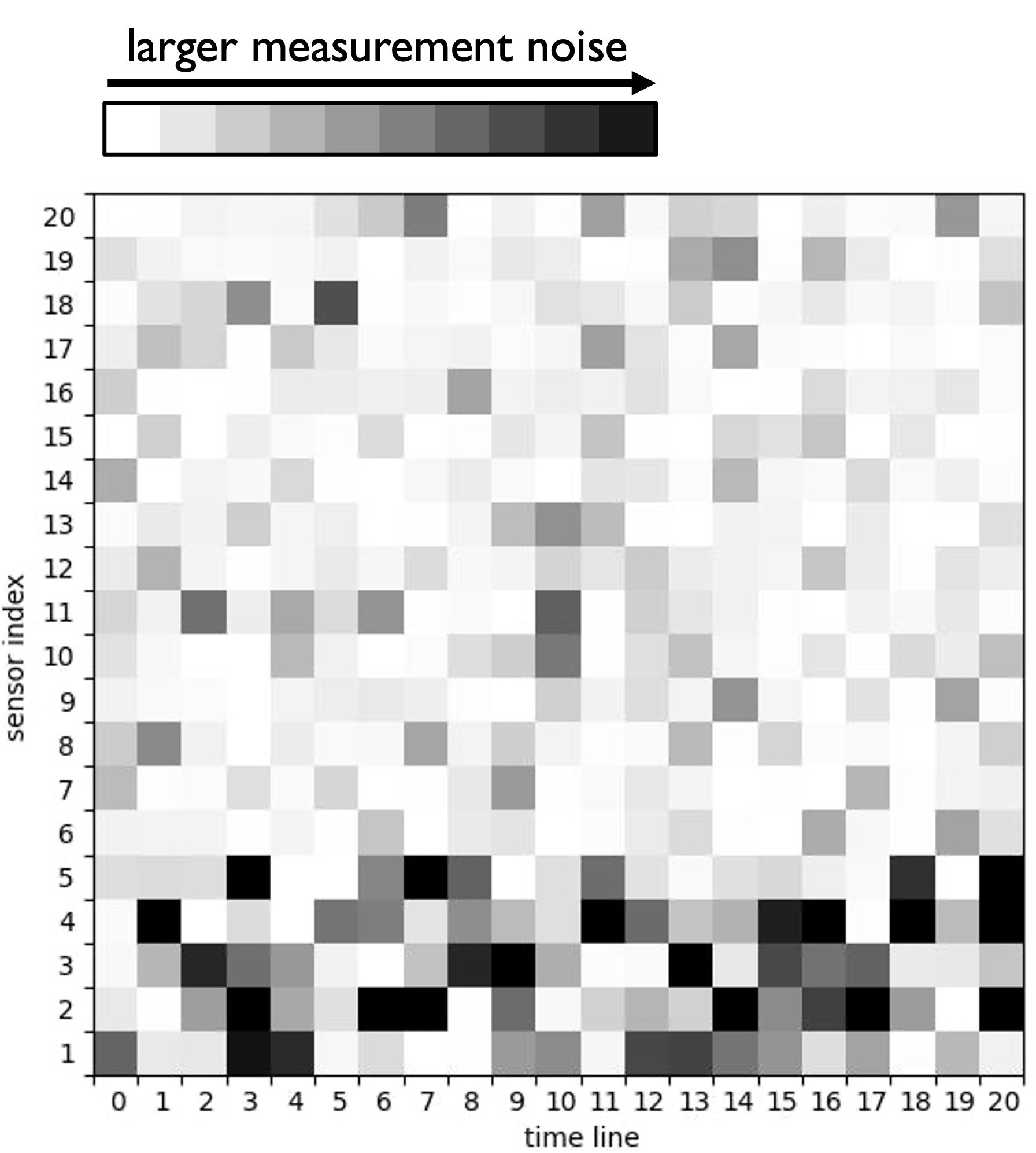
(b) map of observation noise

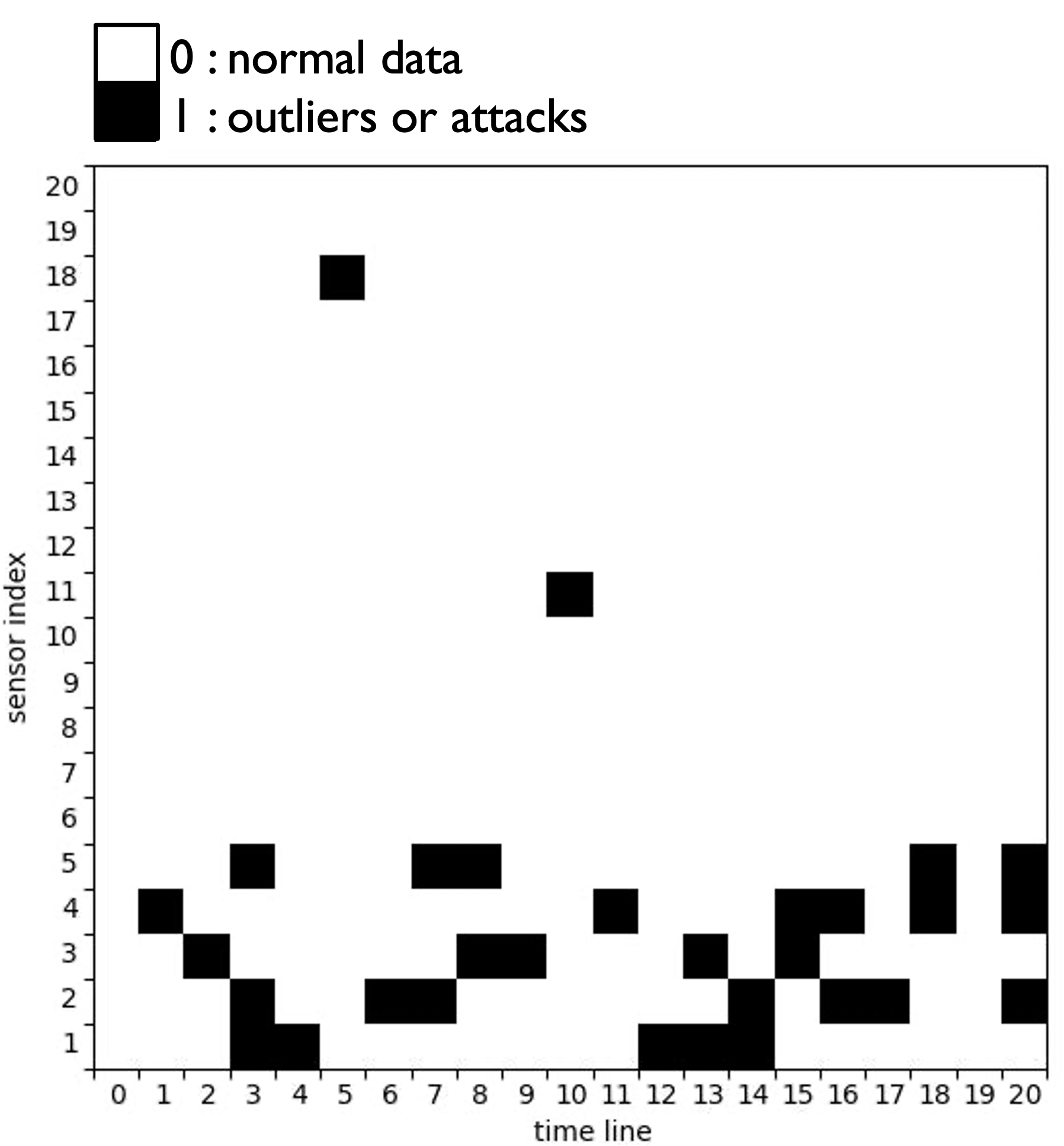
(c) map of estimated indicators

Figure 10: Characterization the measurement error by estimated observation indicators. (b) shows the true observation errors $\|y_{i,j}-C_{j}x_{i}\|^{2}_{R_{j}^{-1}}$, which are continuous values. Sensor $1$ to $5$, under attack, generated a large number of observations with significant errors. (c) shows our assessment of the reliability of each observation, which is boolean.

Comparing Fig. 10(b) and Fig. 10(c), their similarity illustrates that Gaussian-Bernoulli secure estimator effectively characterizes observation errors through indicators. Based on the estimated indicator sequence of each sensor, we can further distinguish between outliers and attacks.

VIII Conclusion

This paper has addressed the problem of sensor security by introducing a GBS estimator, which enables safety in terms of resilient estimation and attack detection. A dual-variable optimization problem, formulated as Problem 1, aims to estimate system states and sensor status using a Gaussian-Bernoulli observation model with indicators.

Starting from the Problem 2, we identify two practical state estimation problems underlying it: sequential state estimation with partial observations and estimation updates with disordered new observations. We then propose and derive direct and iterative state estimation methods based on the equivalent Problem 3 and Problem 4, which are suitable for different observation update patterns. Finally, we introduce the GBS estimator algorithm to solve Problem 1 and prove the existence and convergence of the solution.

In experiments, we compare the direct and iterative methods under different update patterns, simulate various sensor attacks, and show the GSB estimator’s superior detection and estimation. Lastly, we demonstrate that our Boolean indicator accurately matches actual observation errors.

Since the Gaussian-Bernoulli mixture model can effectively model systems that involve decision-making tasks, future work will focus on how to apply it to other control problems. One potential direction is to identify the system parameters while balancing the selection of effective data and the estimation of system parameters. These efforts will help us incorporate discrete objectives into the continuous system states.

Appendix A

A-A Proof of Lemma 1

Lemma 1 extends the conclusions of Kalman filtering to the optimal estimation of state sequences under partial observation sequences.

We begin by deriving the optimal estimation based on the past observation sequences. When the selected index set $\mathcal{O}$ is determined, each state $x_{t}$ corresponds to a sequence containing past observations $\mathcal{O}_{t}=\{i|i\in\mathcal{O},i\leq t\}$ and the estimated state $\hat{x}_{t|\mathcal{O}_{t}}$. Define Kalman innovation as $e_{t}=y_{t}-C\hat{x}_{t|\mathcal{O}_{t-1}}$, which can be regarded as the “new information” about systematic randomness.

In Kalman filtering, the optimal state estimate can be calculated through the following process with $\hat{x}_{0|\emptyset}=0$.

$$\left\{\begin{matrix}e_{t}=y_{t}-C\hat{x}_{t|\mathcal{O}_{t-1}}\\ \hat{x}_{t|\mathcal{O}_{t}}=\hat{x}_{t|\mathcal{O}_{t-1}}+K_{t}e_{t}\\ \hat{x}_{t+1|\mathcal{O}_{t}}=A\hat{x}_{t|\mathcal{O}_{t}}\end{matrix}\right.$$ (35)

where $K_{t}=0$ if $t\notin\mathcal{O}$.

By rewriting the Kalman filter equation as

$$\left\{\begin{matrix}\hat{x}_{t+1|\mathcal{O}_{t}}=A\hat{x}_{t|\mathcal{O}_{t-1}}+AK_{t}e_{t},\\ y_{t}=C\hat{x}_{t|\mathcal{O}_{t-1}}+e_{t},\end{matrix}\right.$$ (36)

we have another state-space model for the process $\{y_{t}\}$. Based on the equation (36),

$$y_{t} =C(A\hat{x}_{t-1|\mathcal{O}_{t-2}}+AK_{t-1}e_{t-1})+e_{t}$$

$$=CA\hat{x}_{t-1|\mathcal{O}_{t-2}}+(CAK_{t-1}e_{t-1}+e_{t})=\cdots$$

$$=\sum_{i=0}^{t-1}CA^{t-i}K_{i}e_{i}+e_{t}.$$ (37)

Therefore, defining the column vector $E_{\mathcal{O}}=col\{e_{0},e1,\cdots,e_{N}\}$, we can relate $Y$ and $E$ as $Y=L_{\mathcal{O}}E_{\mathcal{O}}$, where

$$L_{\mathcal{O}} =\begin{bmatrix}I&0&\cdots&0\\ C\Phi(1)K_{0}&I&\cdots&0\\ \vdots&\vdots&\vdots&\vdots\\ C\Phi(N)K_{0}&C\Phi(N-1)K_{1}&\cdots&I\end{bmatrix},$$ (38)

and $\Phi(k)=A^{k}$.

We note also that the inverse matrix $L^{*}_{\mathcal{O}}$, which satisfies $E_{\mathcal{O}}=L^{*}_{\mathcal{O}}Y$, can be found as

$$L^{*}_{\mathcal{O}} =\begin{bmatrix}I&0&\cdots&0\\ -CAK_{0}&I&\cdots&0\\ \vdots&\vdots&\vdots&\vdots\\ -C\Phi_{p}(N,1)K_{0}&-C\Phi_{p}(N,2)K_{1}&\cdots&I\end{bmatrix},$$ (39)

where $\Phi_{p}(k,j)=\prod_{i=j}^{k-1}A(I-K_{i}C)$.

An alternative expression of the innovation model can be obtained

$$\hat{x}_{t|\mathcal{O}_{t}}=A\hat{x}_{t-1|\mathcal{O}_{t-1}}+K_{t}e_{t}.$$ (40)

Defining the column vector $\bar{X}_{\mathcal{O}}=col\{\hat{x}_{0|\mathcal{O}_{0}},\hat{x}_{1|\mathcal{O}_{1}},\cdots,\hat{x}_{N|\mathcal{O}_{N}}\}$. We can relate $E_{\mathcal{O}}$ and $\bar{X}_{\mathcal{O}}$ as $\bar{X}_{\mathcal{O}}=M_{\mathcal{O}}E_{\mathcal{O}}$, where

$$M_{\mathcal{O}} =\begin{bmatrix}K_{0}&0&\cdots&0\\ \Phi(1)K_{0}&K_{1}&\cdots&0\\ \vdots&\vdots&\vdots&\vdots\\ \Phi(N)K_{0}&\Phi(N-1)K_{1}&\cdots&K_{N}\end{bmatrix}$$ (41)

Next, we aim to switch the $\bar{X}_{\mathcal{O}}$ to $\hat{X}_{\mathcal{O}}$. For the RTS smoother provides the future information backwards,

$$\hat{x}_{t|\mathcal{O}}=\hat{x}_{t|\mathcal{O}_{t}}+F_{t}(\hat{x}_{t+1|\mathcal{O}}-A\hat{x}_{t|\mathcal{O}_{t}}),$$ (42)

we can relate $\bar{X}_{\mathcal{O}}$ and $\hat{X}_{\mathcal{O}}$ as $\hat{X}_{\mathcal{O}}=H_{\mathcal{O}}\bar{X}_{\mathcal{O}}$, where

$$H_{\mathcal{O}} =\begin{bmatrix}I-F_{0}\Phi(N)&\cdots&\cdots&F_{0}...F_{N-1}\\ \vdots&\vdots&\vdots&\vdots\\ 0&0&I-F_{N-1}\Phi(1)&F_{N-1}\\ 0&0&0&I\end{bmatrix}.$$ (43)

Ultimately, we derive the optimal linear estimate under condition $\mathcal{O}$.

$$\hat{X}_{\mathcal{O}}=K_{\mathcal{O}}Y=H_{\mathcal{O}}M_{\mathcal{O}}L^{*}_{\mathcal{O}}Y$$ (44)

Observations contribute different weight to each state estimate, with the element of matrix $K_{\mathcal{O}}$ representing the optimal allocation of weights. For those observations $\{y_{t}|t\notin\mathcal{O}\}$, their weights in $K_{\mathcal{O}}$ equal to $0$. As the set $\mathcal{O}$ changes, the corresponding optimal weights will also change.

A-B Proof of Theorem 2

We begin by deriving a bound on smoothness of $\phi(x)$ at which composite gradient mapping is small if primal suboptimality is small in proposition 3. Similarly, we have the result for strongly convex problems in proposition 3, which implies that a small composite gradient mapping implies a small primal suboptimality. Finally, we apply the proposition and prove the Theorem 2.

Define the composite gradient mapping as

$$\mathbf{D}_{\eta,g}f(x)=\frac{1}{\eta}\left(x-prox_{\eta g}(x-\eta\nabla f(x))\right).$$ (45)

and $x^{+}=\text{prox}_{\eta g}(x-\eta\nabla f(x))$.

Proposition 2.

Assume $f(x)$ is $L$-smooth, and $g(x)$ is $\lambda^{\prime}$ strongly convex. Given a learning rate $\eta>0$ such that $\eta<\frac{2}{(L-\lambda^{\prime})}$, we have

$$\|D_{\eta,g}f(x)\|_{2}^{2}\leq\frac{2/\eta}{2-\eta(L-\lambda^{\prime})}\left[\phi(x)-\phi(x^{+})\right].$$ (46)

Proof. Let

$$Q(z)=f(x)+\nabla f(x)^{T}(z-x)+\frac{1}{2\eta}\|z-x\|_{2}^{2}+g(z),$$ (47)

then $x^{+}$ is the solution of $\min_{z}Q(z)$, and $Q(z)$ is $(\eta^{-1}+\lambda^{\prime})$ strongly convex. This implies that

$$Q(x)-Q(x^{+})\geq\frac{\eta^{-1}+\lambda^{\prime}}{2}\|x-x^{+}\|_{2}^{2}.$$ (48)

Moreover, by the smoothness of $f$, we have

$$\phi(x^{+}) =f(x^{+})+g(x^{+})$$

$$\leq f(x)+\nabla f(x)^{T}(x^{+}-x)+\frac{L}{2}\|x^{+}-x\|_{2}^{2}+g(x^{+})$$

$$=Q(x^{+})+\frac{L-\eta^{-1}}{2}\|x^{+}-x\|_{2}^{2}$$

$$\leq Q(x)+\frac{L-\lambda^{\prime}-2\eta^{-1}}{2}\|x^{+}-x\|_{2}^{2}$$

$$=\phi(x)+\frac{L-\lambda^{\prime}-2\eta^{-1}}{2}\|\eta D_{\eta,g}f(x)\|_{2}^{2},$$ (49)

which implies the result.

Proposition 3.

Assume that $f(x)$ is an $L$-smooth convex function and $\phi(x)$ is $\lambda_{\phi}$ strongly convex. Given a learning rate $\eta>0$, we have

$$\phi(x^{+})\leq\phi(x_{*})+\frac{(1-\eta L)^{2}}{2\lambda_{\phi}}\|D_{\eta,g}f(x)\|_{2}^{2}.$$ (50)

Proof. For $x^{+}$ is the solution of (47), we obtain the following first order condition. For all $x_{*}$,

$$[\nabla f(x)+\nabla g(x^{+})+\eta^{-1}(x^{+}-x)]^{T}(x_{*}-x^{+})\geq 0.$$ (51)

This implies that

$$[\nabla f(x^{+})+\nabla g(x^{+})]^{T}(x_{*}-x^{+})$$

$$= [\nabla f(x^{+})-\nabla f(x)]^{T}(x_{*}-x^{+})$$

$$+[\nabla f(x)+\nabla g(x^{+})]^{T}(x_{*}-x^{+})$$

$$\geq [\nabla f(x^{+})-\nabla f(x)]^{T}(x_{*}-x^{+})$$

$$+\eta^{-1}(x-x^{+})^{T}(x_{*}-x^{+})$$

$$= [\nabla\tilde{f}(x^{+})-\nabla\tilde{f}(x)]^{T}(x_{*}-x^{+})$$

$$\geq -\|L-\eta^{-1}\|\cdot\|x^{+}-x\|_{2}\cdot\|x^{+}-x_{*}\|_{2},$$ (52)

where $\hat{f}(z)=f(z)-0.5\eta^{-1}\|z\|_{2}^{2}$.

Derived from the strong convexity of $\phi(x)$, we can have the following inequality.

$$(\nabla f(x^{+})+\nabla g(x^{+}))^{T}(x_{*}-x^{+})$$

$$\leq\phi(x_{*})-\phi(x^{+})-\frac{\lambda_{\phi}}{2}\|x_{*}-x^{+}\|_{2}^{2}.$$ (53)

Taking the inequality (52) and (53) into consideration, we can infer that

$$\phi(x_{*})-\phi(x^{+})$$

$$\geq \inf_{z}\left[\frac{\lambda_{\phi}}{2}\|z-x^{+}\|_{2}^{2}-|L-\eta^{-1}|\|x^{+}-x\|_{2}\|x^{+}-z\|_{2}\right]$$

$$= \frac{(\eta^{-1}-L)^{2}}{2\lambda_{\phi}}\|x^{+}-x\|_{2}^{2}=\frac{(1-\eta L)^{2}}{2\lambda_{\phi}}\|D_{\eta,g}f(x)\|_{2}^{2}.$$ (54)

Main Proof. We can define

$$Q_{t}(x)=f(x_{t-1}) +\nabla f(x_{t-1})^{T}(x-x_{t-1})$$

$$+\frac{1}{2\eta_{t}}\|x-x_{t-1}\|_{2}^{2}+g(x).$$ (55)

Then $x_{t}=\text{prox}_{\eta_{t}g}(x_{t-1}-\eta_{t}\nabla f(x_{t-1}))$.

Due to Proposition 2, we have the following derivation

$$\phi(x_{t})\leq Q_{t}(x_{t})\leq Q_{t}(x)-\frac{\eta_{t}^{-1}+\lambda^{\prime}}{2}\|x-x_{t}\|_{2}^{2}$$

$$\leq f(x)-\frac{\lambda}{2}\|x-x_{t-1}\|_{2}^{2}+\frac{1}{2\eta_{t}}\|x-x_{t-1}\|_{2}^{2}+g(x)$$

$$-\frac{\eta_{t}^{-1}+\lambda^{\prime}}{2}\|x-x_{t}\|_{2}^{2}$$

$$= \phi(x)+\frac{1}{2}\left(\frac{1}{\eta_{t}}-\lambda\right)\|x-x_{t-1}\|_{2}^{2}$$

$$-\frac{\eta_{t}^{-1}+\lambda^{\prime}}{2}\|x-x_{t}\|_{2}^{2}.$$ (56)

Let $x=x_{t-1}+\theta(\bar{x}-x_{t-1})$ for some $\theta\in(0,1)$, we have

$$(1-\theta)\phi(x_{t-1})+\theta\phi(\bar{x})-\phi(x)$$

$$= (1-\theta)[\phi(x_{t-1})-\phi(x)-\nabla\phi(x)^{T}(x_{t-1}-x)]$$

$$+\theta[\phi(\bar{x})-\phi(x)-\nabla\phi(x)^{T}(\bar{x}-x)]$$

$$\geq (1-\theta)\frac{\lambda+\lambda^{\prime}}{2}\|x_{t-1}-x\|_{2}^{2}+\theta\frac{\lambda+\lambda^{\prime}}{2}\|\bar{x}-x\|_{2}^{2}$$

$$= (1-\theta)\theta\frac{\lambda+\lambda^{\prime}}{2}\|\bar{x}-x_{t-1}\|_{2}^{2}.$$ (57)

The inequality is due to the $\lambda+\lambda^{\prime}$ strong convexity of $\phi(x)$. Therefore

$$\phi(x_{t}) \leq(1-\theta)\phi(x_{t-1})+\theta\phi(\bar{x})$$

$$\quad-\theta(1-\theta)\frac{\lambda+\lambda^{\prime}}{2}\|\bar{x}-x_{t-1}\|_{2}^{2}$$

$$\quad+\frac{\theta^{2}}{2}\left(\frac{1}{\eta_{t}}-\lambda\right)\|\bar{x}-x_{t-1}\|_{2}^{2}.$$ (58)

Taking $\eta_{t}=\eta$ and $\theta=(\lambda+\lambda^{\prime})/(\lambda^{\prime}+\eta^{-1})$, we obtain

$$\phi(x_{t})\leq(1-\theta)\phi(x_{t-1})+\theta\phi(\bar{x}).$$ (59)

which implies the result.

A-C Proof of Theorem 3

Theorem 3 explains the relationship between the initial estimation error and the iteration number. We first investigate how the state estimation at the corresponding moment is updated when the new observation is added in Proposition 4. Based on this result, we derive the maximum number of iterations.

Proposition 4.

Assume that the optimal state estimation of $x_{k}$ under $y_{\mathcal{O}}$ is $\hat{x}_{k|\mathcal{O}}$ and the error covariance is $P_{k|\mathcal{O}}$. When the observation set changes from $y_{\mathcal{O}}$ to $y_{\mathcal{O^{*}}}=y_{\mathcal{O}}\cup\{y_{k}\}$, the optimal state estimation of $x_{k}$ is updated by

$$\hat{x}_{k|\mathcal{O}^{*}}=\hat{x}_{k|\mathcal{O}}+P_{k|\mathcal{O}}C^{T}(CP_{k|\mathcal{O}}C^{T}+R)^{-1}(y_{k}-C\hat{x}_{k|\mathcal{O}})$$ (60)

Proof. Denote the linear space $S_{\mathcal{O}}=Span\{y_{\mathcal{O}}\}$. Define the inner product of two random vectors as $\left\langle x,y\right\rangle=E[xy^{T}]$. And also define the estimation error as $\tilde{x}_{k|\mathcal{O}}=x_{k}-\hat{x}_{k|\mathcal{O}}$.

For $\hat{x}_{k|\mathcal{O}}$ is the optimal state estimation under $y_{\mathcal{O}}$, it has following properties.

$$\hat{x}_{k|\mathcal{O}} =\text{Proj}\{x_{k}|S_{\mathcal{O}}\}$$ (61)

$$\hat{x}_{k|\mathcal{O}} \perp(x_{k}-\hat{x}_{k|\mathcal{O}})$$ (62)

$$S_{\mathcal{O}} \perp(y_{k}-C\hat{x}_{k|\mathcal{O}})$$ (63)

$$Span\{y_{\mathcal{O}},y_{k}\} =Span\{y_{\mathcal{O}},(y_{k}-C\hat{x}_{k|\mathcal{O}})\}$$ (64)

Therefore, we can calculate the $\hat{x}_{k|\mathcal{O}^{*}}$ as follows:

$$\hat{x}_{k|\mathcal{O}^{*}} =\text{Proj}\{x_{k}|S_{\mathcal{O}^{*}}\}$$

$$=\text{Proj}\{x_{k}|S_{\mathcal{O}}\}+\text{Proj}\{x_{k}|(y_{k}-C\hat{x}_{k|\mathcal{O}})\}$$

$$=\hat{x}_{k|\mathcal{O}}+\frac{\left\langle x_{k},y_{k}-C\hat{x}_{k|\mathcal{O}}\right\rangle(y_{k}-C\hat{x}_{k|\mathcal{O}})}{\left\langle y_{k}-C\hat{x}_{k|\mathcal{O}},y_{k}-C\hat{x}_{k|\mathcal{O}}\right\rangle}$$

$$=\hat{x}_{k|\mathcal{O}}+\frac{\left\langle\tilde{x}_{k|\mathcal{O}}+\hat{x}_{k|\mathcal{O}},C\tilde{x}_{k|\mathcal{O}}+v_{k}\right\rangle}{\left\langle C\tilde{x}_{k|\mathcal{O}}+v_{k},C\tilde{x}_{k|\mathcal{O}}+v_{k}\right\rangle}(y_{k}-C\hat{x}_{k|\mathcal{O}})$$

$$=\hat{x}_{k|\mathcal{O}}+\frac{\left\langle\tilde{x}_{k|\mathcal{O}},C\tilde{x}_{k|\mathcal{O}}\right\rangle}{\left\langle C\tilde{x}_{k|\mathcal{O}},C\tilde{x}_{k|\mathcal{O}}\right\rangle+\left\langle v_{k},v_{k}\right\rangle}(y_{k}-C\hat{x}_{k|\mathcal{O}})$$

$$=\hat{x}_{k|\mathcal{O}}+P_{k|\mathcal{O}}C^{T}(CP_{k|\mathcal{O}}C^{T}+R)^{-1}(y_{k}-C\hat{x}_{k|\mathcal{O}})$$ (65)

Main Proof. Assume the $\arg\min_{\hat{x}_{0:N}}\phi_{\mathcal{O}}=\hat{x}_{0:N|\mathcal{O}}$ and $\arg\min_{\hat{x}_{0:N}}\phi_{\mathcal{O}^{*}}=\hat{x}_{0:N|\mathcal{O}^{*}}$. The objective function with new observation $y_{k}$ can be defined as:

$$\phi_{\mathcal{O}^{*}}(\hat{x}_{0:N})=\phi_{\mathcal{O}}(\hat{x}_{0:N})+\|y_{k}-C\hat{x}_{k}\|^{2}_{R^{-1}}.$$ (66)

This implies that

$$\phi_{\mathcal{O}^{*}}(\hat{x}_{0:N|\mathcal{O}})= \phi_{\mathcal{O}}(\hat{x}_{0:N|\mathcal{O}})+\|y_{k}-C\hat{x}_{k|\mathcal{O}}\|^{2}_{R^{-1}}$$

$$\leq \phi_{\mathcal{O}}(\hat{x}_{0:N|\mathcal{O}^{*}})+\|y_{k}-C\hat{x}_{k|\mathcal{O}}\|^{2}_{R^{-1}}$$

$$= \phi_{\mathcal{O}}(\hat{x}_{0:N|\mathcal{O}^{*}})+\|y_{k}-C(\hat{x}_{k|\mathcal{O}^{*}}-\Delta x_{k})\|^{2}_{R^{-1}}$$

$$\leq \phi_{\mathcal{O}}(\hat{x}_{0:N|\mathcal{O}^{*}})+\|y_{k}-C\hat{x}_{k|\mathcal{O}^{*}}\|^{2}_{R^{-1}}$$

$$+\|C\Delta x_{k}\|^{2}_{R^{-1}}+2\|C\Delta x_{k}\|\|y_{k}-C\hat{x}_{k|\mathcal{O}^{*}}\|$$

$$\leq \min\phi_{\mathcal{O}^{*}}(\hat{x}_{0:N})+\|C\Delta x_{k}\|^{2}_{R^{-1}}$$

$$+2\|C\Delta x_{k}\|_{R^{-1}}\|y_{k}-C\hat{x}_{k|\mathcal{O}}\|_{R^{-1}}$$ (67)

where $\Delta x_{k}$ can be substituted by equation (65).

When the initial value $\hat{X}^{0}=col\{\hat{x}_{0:N|\mathcal{O}}\}$, we have

$$\phi_{\mathcal{O}^{*}}(\hat{X}^{0})-\min\phi_{\mathcal{O}^{*}}(\hat{X})$$

$$\leq (\|C\Delta x_{k}\|^{2}_{R^{-1}}+2\|C\Delta x_{k}\|_{R^{-1}}\|y_{k}-C\hat{x}_{k|\mathcal{O}^{*}}\|_{R^{-1}})$$ (68)

Based on the Theorem 2, we can imply the result.

Appendix B

B-A The limitation of $\chi^{2}$ based method

Consider a scalar system with single sensor at interval $T=[0,20]$, where $x_{0}\sim\mathcal{N}(0,1),A=1,C=1,Q=0.5,R=1.$ We simulate sensors in three different status, as shown in Fig. 11.

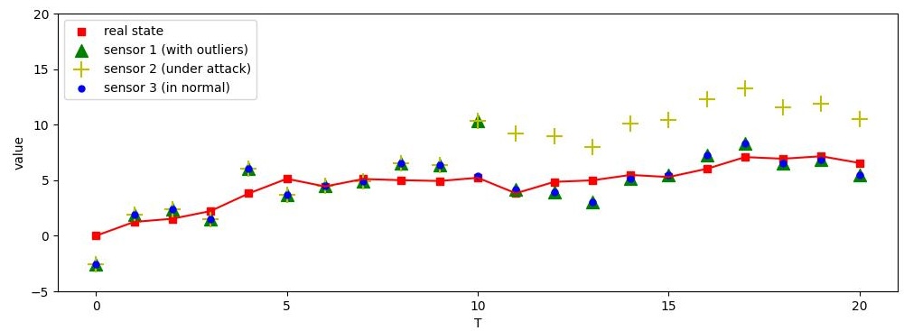
(a) three different sensor status

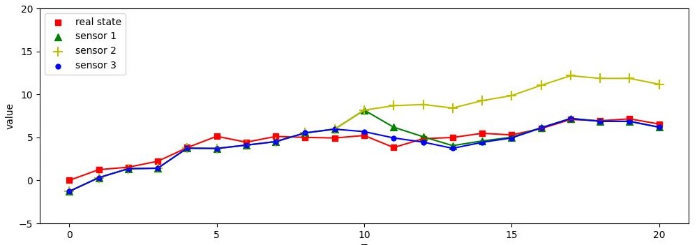
(b) state estimation from different sensors

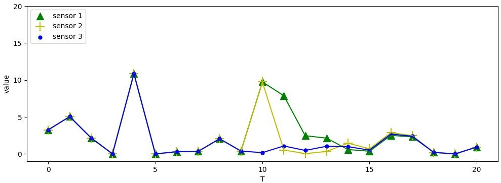
(c) $\chi^{2}$ sequences from different sensors

Figure 11: Illustration of the limitation of $\chi^{2}$ based method. (a) displays three sets of sensor data: the blue represents normal observations. Compared to the blue observation, the green shows a deviation only at $t=10$, while the yellow deviates after $t=10$. (b)(c) shows their corresponding state estimates and $\chi^{2}_{t}$ values.

The experiment indicates that although the state estimates from Sensor 2 and Sensor 1 are very different, their $\chi^{2}$ curves are quite similar. This similarity arises because, after $t=10$, the state estimate from Sensor 2 becomes inaccurate, rendering the $\chi^{2}$ curve unreliable. Additionally, this phenomenon complicates the distinction between outliers and attacks, thus reducing the success rate of attack detection.

B-B Additional experiments with different algorithm parameters

Under different parameters, the algorithm’s estimation performance is roughly the same as shown in Fig. 9. The detection success rates corresponding to different parameters are illustrated in Fig. 12.

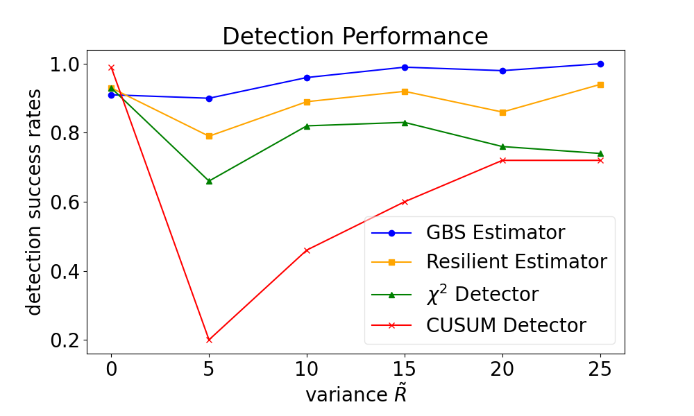
$\alpha_{\text{threshold}}=6,\tau_{\text{tolerant}}=2$

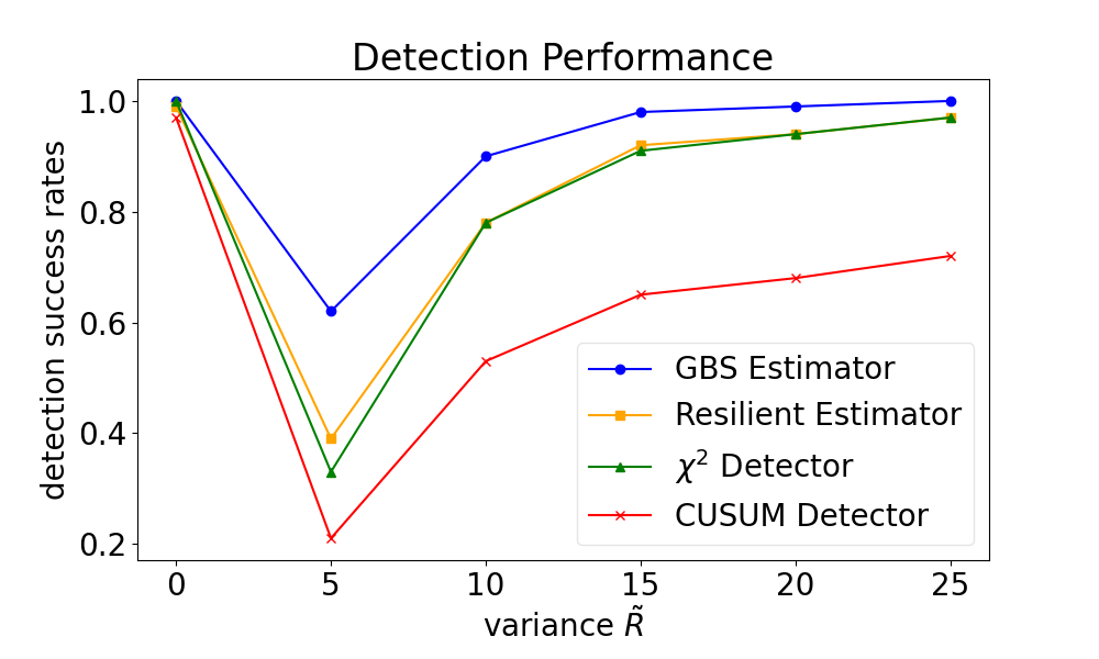
$\alpha_{\text{threshold}}=6,\tau_{\text{tolerant}}=4$

(a) random interference attack with different intensity

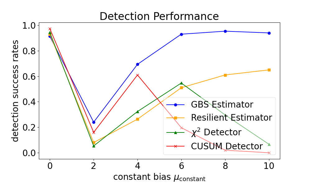
$\alpha_{\text{threshold}}=6,\tau_{\text{tolerant}}=2$

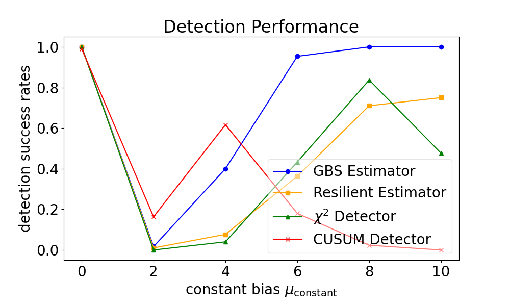
$\alpha_{\text{threshold}}=6,\tau_{\text{tolerant}}=4$

(b) constant bias attack with different intensity

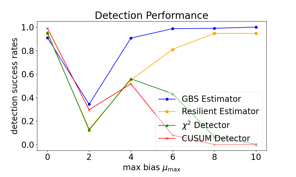
$\alpha_{\text{threshold}}=6,\tau_{\text{tolerant}}=2$

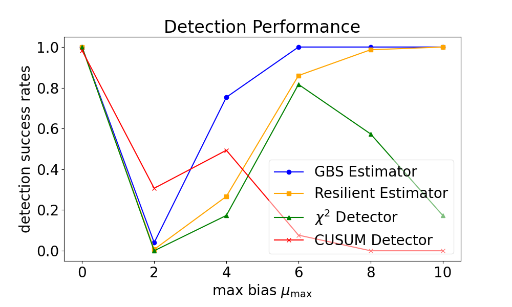
$\alpha_{\text{threshold}}=6,\tau_{\text{tolerant}}=4$

(c) uniformly increasing bias attack with different intensity

Figure 12: Comparison of GSB Estimator’s performance with other algorithms under different types of attacks and varying intensities. In the left figure, we compare the detection success rate with other algorithms. In the right figure, we compare the estimation error with other algorithms.

Xingzhou Chen received his B.E. degree in the Department of Control Science and Engineering from Zhejiang University, Hangzhou, China, in 2021. He is currently working towards the Ph.D. degree in the Department of Electronic and Computer Engineering at the Hong Kong University of Science and Technology, Hong Kong. He also worked as a research intern at Huawei Noah’s Ark Lab, HongKong, and Tencent Robotics X Lab, Shenzhen. His research mainly focuses on control theory and its applications in Robotics.

Nachuan Yang received his B.Sc. degree in Mathematics from the University of Hong Kong and Ph.D. degree in Electronic and Computer Engineering from the Hong Kong University of Science and Technology, Hong Kong. He is currently a Postdoctoral Researcher at the University of Alberta, AB, Canada. From June 2019 to August 2019, he was a visiting student at the Department of Applied Mathematics, Cornell University, NY, USA. From June 2020 to July 2020, he was a visiting engineer at Huawei Cloud BU, Shenzhen. His research mainly focuses on control theory and its applications in cyber-physical systems.

Peihu Duan received the B.E. degree in Mechanical Engineering from Huazhong University of Science and Technology, Wuhan, China, in 2015. He received the Ph.D. degree in Mechanical Systems and Control from Peking University, Beijing, China, in 2020. Currently, he works as a Postdoc at School of Electrical Engineering and Computer Science, KTH Royal Institute of Technology, Stockholm, Sweden. From October 2020 to October 2022, he was a Postdoc at the Hong Kong University of Science and Technology and the University of Hong Kong, Hong Kong, China, respectively. His research interests include cooperative and data-driven control and state estimation of networked systems.

Shilei Li received the B.E. degree in Detection Guidance and Control Technology and M.S. degree in Control Engineering both from Harbin Institute of Technology, Harbin, China, in 2015 and 2018 respectively, and the Ph.D. degree in Electronic and Computer Engineering from The Hong Kong University of Science and Technology, Hong Kong, China, in 2022. Currently, he is an assistant professor at the School of Automation, Beijing Institute of Technology, China. His research interests include robust Kalman filtering, orientation estimation of IMUs, synchronization control, human-robot interaction, and exoskeletons.

Ling Shi received his B.E. degree in Electrical and Electronic Engineering from The Hong Kong University of Science and Technology (HKUST) in 2002 and Ph.D. degree in Control and Dynamical Systems from The California Institute of Technology (Caltech) in 2008. He is currently a Professor in the Department of Electronic and Computer Engineering at HKUST. His research interests include cyber-physical systems security, networked control systems, sensor scheduling, event-based state estimation, and multi-agent robotic systems (UAVs and UGVs). He served as an editorial board member for the European Control Conference 2013-2016. He was a subject editor for International Journal of Robust and Nonlinear Control (2015-2017), an associate editor for IEEE Transactions on Control of Network Systems (2016-2020), an associate editor for IEEE Control Systems Letters (2017-2020), and an associate editor for a special issue on Secure Control of Cyber Physical Systems in IEEE Transactions on Control of Network Systems (2015-2017). He also served as the General Chair of the 23rd International Symposium on Mathematical Theory of Networks and Systems (MTNS 2018). He is a member of the Young Scientists Class 2020 of the World Economic Forum (WEF), and he is an IEEE fellow.

References

• [1] J. Giraldo, D. Urbina, A. Cardenas, J. Valente, M. Faisal, J. Ruths, N. O. Tippenhauer, H. Sandberg, and R. Candell, “A survey of physics-based attack detection in cyber-physical systems,” ACM Computing Surveys, vol. 51, no. 4, pp. 1–36, 2018.
• [2] J. C. Jensen, D. H. Chang, and E. A. Lee, “A model-based design methodology for cyber-physical systems,” in IEEE Proceedings of the 7th International Wireless Communications and Mobile Computing Conference, 2011, pp. 1666–1671.
• [3] H. Chen, “Applications of cyber-physical system: a literature review,” Journal of Industrial Integration and Management, vol. 2, no. 03, p. 1750012, 2017.
• [4] X. Yu and Y. Xue, “Smart grids: A cyber–physical systems perspective,” Proceedings of the IEEE, vol. 104, no. 5, pp. 1058–1070, 2016.
• [5] Q. Zhu and T. Basar, “Game-theoretic methods for robustness, security, and resilience of cyberphysical control systems: games-in-games principle for optimal cross-layer resilient control systems,” IEEE Control Systems Magazine, vol. 35, no. 1, pp. 46–65, 2015.
• [6] O. Kocabas, T. Soyata, and M. K. Aktas, “Emerging security mechanisms for medical cyber physical systems,” IEEE/ACM Transactions on Computational Biology and Bioinformatics, vol. 13, no. 3, pp. 401–416, 2016.
• [7] H. He and J. Yan, “Cyber-physical attacks and defences in the smart grid: a survey,” IET Cyber-Physical Systems: Theory & Applications, vol. 1, no. 1, pp. 13–27, 2016.
• [8] K. Kim, J. S. Kim, S. Jeong, J.-H. Park, and H. K. Kim, “Cybersecurity for autonomous vehicles: Review of attacks and defense,” Computers & Security, vol. 103, p. 102150, 2021.
• [9] A. Ruegamer, D. Kowalewski et al., “Jamming and spoofing of GNSS signals–an underestimated risk?!” Proc. Wisdom Ages Challenges Modern World, vol. 3, pp. 17–21, 2015.
• [10] K. Hartmann and C. Steup, “The vulnerability of uavs to cyber attacks-an approach to the risk assessment,” in IEEE Proceedings of the 5th International Conference on Cyber Conflict, 2013, pp. 1–23.
• [11] Y. Mo and B. Sinopoli, “False data injection attacks in control systems,” in Proceedings of the Preprints of the 1st workshop on Secure Control Systems, vol. 1, 2010.
• [12] K. Sonar and H. Upadhyay, “A survey: DDOS attack on internet of things,” International Journal of Engineering Research and Development, vol. 10, no. 11, pp. 58–63, 2014.
• [13] Z. Guo, D. Shi, K. H. Johansson, and L. Shi, “Optimal linear cyber-attack on remote state estimation,” IEEE Transactions on Control of Network Systems, vol. 4, no. 1, pp. 4–13, 2016.
• [14] H. Zhang, P. Cheng, L. Shi, and J. Chen, “Optimal denial-of-service attack scheduling with energy constraint,” IEEE Transactions on Automatic Control, vol. 60, no. 11, pp. 3023–3028, 2015.
• [15] Y. Mo, R. Chabukswar, and B. Sinopoli, “Detecting integrity attacks on scada systems,” IEEE Transactions on Control Systems Technology, vol. 22, no. 4, pp. 1396–1407, 2013.
• [16] C. Murguia and J. Ruths, “Characterization of a cusum model-based sensor attack detector,” in IEEE Proceedings of the 55th Conference on Decision and Control, 2016, pp. 1303–1309.
• [17] C. A. Lowry, W. H. Woodall, C. W. Champ, and S. E. Rigdon, “A multivariate exponentially weighted moving average control chart,” Technometrics, vol. 34, no. 1, pp. 46–53, 1992.
• [18] Y. Li, D. E. Quevedo, S. Dey, and L. Shi, “Sinr-based dos attack on remote state estimation: A game-theoretic approach,” IEEE Transactions on Control of Network Systems, vol. 4, no. 3, pp. 632–642, 2016.
• [19] R. Meira-Góes, S. Lafortune, and H. Marchand, “Synthesis of supervisors robust against sensor deception attacks,” IEEE Transactions on Automatic Control, vol. 66, no. 10, pp. 4990–4997, 2021.
• [20] Y. Mo, S. Weerakkody, and B. Sinopoli, “Physical authentication of control systems: Designing watermarked control inputs to detect counterfeit sensor outputs,” IEEE Control Systems Magazine, vol. 35, no. 1, pp. 93–109, 2015.
• [21] K. Kogiso and T. Fujita, “Cyber-security enhancement of networked control systems using homomorphic encryption,” in IEEE Proceedings of the 54th Conference on Decision and Control, 2015, pp. 6836–6843.
• [22] Q. Lin, S. Adepu, S. Verwer, and A. Mathur, “Tabor: A graphical model-based approach for anomaly detection in industrial control systems,” in Proceedings of the 2018 on Asia Conference on Computer and Communications Security, 2018, pp. 525–536.
• [23] J. Goh, S. Adepu, M. Tan, and Z. S. Lee, “Anomaly detection in cyber physical systems using recurrent neural networks,” in IEEE 18th International Symposium on High Assurance Systems Engineering, 2017, pp. 140–145.
• [24] H. Wang, J. Ruan, Z. Ma, B. Zhou, X. Fu, and G. Cao, “Deep learning aided interval state prediction for improving cyber security in energy internet,” Energy, vol. 174, pp. 1292–1304, 2019.
• [25] Y. Mo and B. Sinopoli, “Secure estimation in the presence of integrity attacks,” IEEE Transactions on Automatic Control, vol. 60, no. 4, pp. 1145–1151, 2014.
• [26] Y. H. Chang, Q. Hu, and C. J. Tomlin, “Secure estimation based Kalman filter for cyber–physical systems against sensor attacks,” Automatica, vol. 95, pp. 399–412, 2018.
• [27] H. Wang, H. Li, J. Fang, and H. Wang, “Robust Gaussian Kalman filter with outlier detection,” IEEE Signal Processing Letters, vol. 25, no. 8, pp. 1236–1240, 2018.