Eccentricities of Close Stellar Binaries

Abstract

Orbits of stellar binaries are in general eccentric. This encodes information about the formation process. Here, we use thousands of main-sequence binaries from the GAIA DR3 catalog to reveal that, binaries inwards of a few AU exhibit a simple Rayleigh distribution with a mode $\sigma_{e}\simeq 0.30$. We find the same distribution for binaries from M to A spectral types, and from tens of days to $10^{3}$days (possibly extending to tens of AU).

This observed distribution is most likely primordial. Its Rayleigh form suggests an origin in weak scattering, while its invariant mode demands a universal process. We experiment with exciting binary eccentricities by ejecting brown dwarfs, and find that the eccentricities reach an equi-partition value of $\sigma_{e}\simeq\sqrt{M_{\rm bd}/M_{*}}$. So to explain the observed mode, these brown dwarfs will have to be of order one tenth the stellar masses, and be at least as abundant in the Galaxy as the close binaries. The veracity of such a proposal remains to be tested.

1 Introduction

Binary stars are common in the Galaxy (Duquennoy & Mayor, 1991; Fischer & Marcy, 1992). Their orbits are invariably eccentric. The distribution of these eccentricities encodes accessible information about their formation, and is a useful property invoked in a wide range of studies. Surprisingly, for binaries closer than tens of AU (’close binaries’), such a fundamental property is not well known.

Multiple lines of evidences suggest two main modes of binary formation (see Duchêne & Kraus, 2013; Offner et al., 2023, for reviews). Wide binaries ($>50$ AU, see, e.g., Parker et al., 2009) likely form following direct collapse of individual components. These are either weakly bound at birth or are captured after birth. Their occurrence is insensitive to or rises with stellar metallicity (El-Badry & Rix, 2019; Hwang et al., 2021), and the two components appear to be randomly paired in mass (Moe & Di Stefano, 2017). Close binaries, on the other hand, are now thought to have formed through gravitational fragmentation in massive circum-stellar disks (see review by Kratter & Lodato, 2016). Their occurrence anti-correlates with stellar metallicity (Moe et al., 2019), and the two masses are correlated (Raghavan et al., 2010; Duchêne & Kraus, 2013; Moe & Di Stefano, 2017) with an excess at equal-mass (’twin-binaries’, Moe & Di Stefano, 2017; El-Badry et al., 2019).

These different formation pathways also manifest in binary eccentricities – a property that is observationally accessible and dynamically informative. Wide binaries are observationally determined to have a thermal distribution ($dN/de\propto e$), as inferred from spectroscopic binaries (Duquennoy & Mayor, 1991; Raghavan et al., 2010) and visual binaries(Tokovinin, 2020; Hwang et al., 2022). This reflects a dynamic past in the birth clusters (Parker et al., 2009), where plentiful scatterings with other stars have relaxed the binaries towards a ’thermal’ equilibrium (Jeans, 1919; Heggie, 1975).

This concordance between theory and observation does not, however, extend to close binaries. There are no theoretical predictions for their e-distribution, owing to the uncertain fragmentation process. On the observational side, their e-distribution remains murky, though it clearly differs from that of the wide binaries. The current wisdom is that they are consistent with being uniform, $dN/de\propto e^{0}$ (Raghavan et al., 2010; Duchêne & Kraus, 2013; Moe & Di Stefano, 2017; Tokovinin, 2000; Geller et al., 2021; Hwang et al., 2022), but this is only a best-guess estimate that is based on small samples and has no ready theoretical explanation.

For instance, selecting from the volume-complete (to 25pc) Solar-type sample (Raghavan et al., 2010; Moe & Di Stefano, 2017), for binaries with periods $10^{2}-10^{3}$d, so as to exclude binaries that may have experienced tidal circularization or may have been disturbed by passing-by stars, we are left with only $18$ binaries. It is clear a much larger sample is sorely needed.

The Gaia mission (Gaia Collaboration et al., 2016, 2023a), especially with its most recent non-single-star catalogue published in DR3 (Gaia Collaboration et al., 2023b), provides just this sample. The GAIA binaries, as we show here, sharpen our vision dramatically. The e-distribution for those inward of a few AU follows, distinctly, a Rayleigh distribution.

2 GAIA Binaries

Here we will study GAIA binaries with eccentricities explicitly determined by astrometry and/or radial velocities. The details of our binary selection are in Appendix A, and a short form is presented in Table 1. The ’full’ main-sequence binary sample includes some $150,000$ systems. We pare down this large set by different cuts (Table 1) and study their respective properties. Among these, we highlight results from the so-called ’gold’ sample, $\sim 3000$ Sun-like binaries that have periods from $10^{2}-10^{3}$ days, and that lie within $150$pc. Binaries with too short a period can be affected by tidal circularization, while DR3 extends to just beyond $10^{3}$ days; binaries beyond $150$pc are incomplete to various degrees (see Appendix B).

sample name	criterion	sample size	best-fit $\sigma_{e}$
DR3 binaries	-	$362,065$	$0.238$
‘Full’	main-sequence, significance $>10$	$147,634$	$0.240$
‘Primordial’	period $P\in[10^{2},10^{3}]$ d	$103,950$	$0.256$
-	‘Orbital’ or ‘AstroSpectroSB1’	$97,458$	$0.258$
-	goodness-of-fit cut (see text)	$90,376$	$0.257$
‘Sun-like’	primary $R_{*}\in[0.7,2.0]R_{\odot}$	$81,107$	$0.258$
‘gold’	distance $<150$pc	$3,071$	$0.303$

Table 1: How we pare down the GAIA binary catalog to obtain various samples in this study. The right-most column lists the best-fit Rayleigh modes. They are most affected by the distance cut.

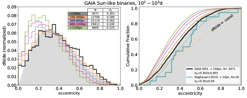
Figure 1: Eccentricity distribution for the GAIA ’Sun-like’ sample (Table 1), split by distances, shown in differential (left panel) and cumulative (right panel) forms. The ’gold’ sample ($<150$pc, thick black lines) is largely free of selection effects and is well described by a Rayleigh distribution with a mode $\sigma_{e}=0.30$ (gray-shaded areas). E-distributions for binaries at larger distances gradually shift to the left, reflecting the increasing severity of selection bias. The right panel also presents the $N=18$ spectroscopic binaries within the same period range (Raghavan et al., 2010). The GAIA gold sample is statistically consistent with this set but firmly rejects the ’uniform’ hypothesis ($dN/de\propto e^{0}$).

The eccentricity distributions of the binary samples are shown in Fig. 1. The data are well described by a Rayleigh distribution,

$$\frac{dN}{de}={e\over{\sigma_{e}^{2}}}\,\exp\left({-\frac{e^{2}}{2\sigma_{e}^{2}}}\right)\,.$$ (1)

For the ’gold’ sample, we find $\sigma_{e}=0.303\pm 0.003$, where the uncertainty accounts for the sample size. For samples lying at larger distances, $\sigma_{e}$ reduces gradually (also see Fig. 5). This reflects the detection bias in GAIA (El-Badry et al., 2024): more eccentric binaries are harder to detect at larger distances, because they spend more time at slowly-moving apoaps, and their photo-centre shifts are smaller at periaps. Fortunately, as we elaborate in Appendix B, the GAIA sample is effectively complete to $150$pc.

Bearing in mind this detection bias, we can employ the $150,000$-strong ’full’ sample to paint a more nuanced picture of the e-distribution.

In Fig. 2, we split the ’full’ sample apart by primary mass (with primary radii from $0.5$ to $3R_{\odot}$, corresponding to spectral types A-F-G-K-M) and by orbital periods (from $2$ days to $1200$d). We adopt the mean eccentricity ($\langle e\rangle$) as a proxy for the Rayleigh mode, where $\langle e\rangle=\sigma_{e}{\sqrt{\pi/2}}$ for a Rayleigh distribution. We find that every bin, with the exception of those that are closer than $\sim 20$d and have therefore undergone various degrees of tidal circularization, exhibits a similar mean eccentricity of $\langle e\rangle\sim 0.31$, or $\sigma_{e}\sim 0.25$. This latter value is close to that obtained for the ’Sun-like’ sample (’gold’ but including all distances), $\sigma_{e}=0.258$, and is a result of convolution between the true mode and detection bias. Assuming the same detection bias across all bins, this exercise suggest that the intrinsic Raleigh mode is invariant, across a wide range of primary spectral types, and over a large span in orbital periods. Such an invariance is remarkable and points to a universal process at work.

Along with this general invariance, we observe a hint that the Rayleigh mode may vary with the binary mass-ratio (Fig. 6). However, a detailed study is needed to exclude an origin in detection bias (Appendix C).

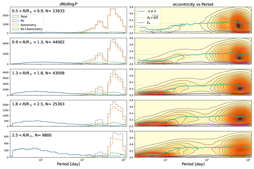
Figure 2: Properties of the ’full’ sample from Table 1, split by primary radii (rows) and orbital periods (x-axis). The left panels show the period distributions, indicating different detection methods. The right panels show kernel density estimation in the $e-\log P$ plane. The effects of tidal circularization are seen for binaries short-ward of $\sim 20$days. But beyond that, all bins reach the same mean-eccentricity ($\langle e\rangle$, green curves), corresponding to a Rayleigh mode of $\sigma_{e}=\langle e\rangle/\sqrt{\pi/2}=0.25$. The low-lying blue curves are the mean eccentricity errors (${\bar{\epsilon}}_{e}$), with individual uncertainties ranging typically from $0.02-0.05$.

Now we put our work on some statistical footing. Adopting a Bayesian framework (Appendix G), we formally establish that the ’gold’ sample strongly favor a model where a single Rayleigh (as opposed to two) describes the data and where the mode is strongly constrained to be $\sigma_{e}=0.30$. Second, the ’gold’ sample is statistically consistent (Fig. 1) with the older, sparse sample ($N=18$ spectroscopic binaries within $10^{2}-10^{3}$d in Raghavan et al., 2010), from which the ’uniform’ e-distribution was deduced. The ’uniform’ guess is the simplest guess based on a small sample, but it is wrong.

Lastly, we hope to gain some insights as to how far out in period the Rayleigh distribution may reach. Tokovinin (2020); Hwang et al. (2022) show that binaries outside $100$AU ($\sim 3\times 10^{5}$d) are thermally distributed in eccentricities ($dN/de\propto e$). What about binaries from $10^{3}$ day to $3\times 10^{5}$d?

We suggest that the Rayleigh distribution likely extends to tens of AU, and where it is gradually replaced by the thermal distribution over the above period range. Part of our argument is based on theoretical prejudice. As a group, close binaries are thought to extend to tens of AU. This is likely determined by the sizes of massive disks (Tobin et al., 2020), and by the scale at which gravitational collapse occurs (Rafikov, 2005; Matzner & Levin, 2005; Kratter et al., 2010). So if all close binaries are formed in disks, the same Rayleigh distribution should be observed out to tens of AU.

We point to two samples that are consistent with this suggestion. One is the sample of long-period ($p=10^{3}-10^{5}$d) spectroscopic or visual binaries from Raghavan et al. (2010). As we argue in Appendix G, a mixture model with roughly equal proportions of Rayleigh and thermal provides a description that is marginally better than a uniform distribution (Fig. 8). The second sample comes from the resolved binaries in GAIA (El-Badry et al., 2021). For those from $10-100$AU, their instantaneous radius-velocity vectors can also be interpreted by the same mixture model (Fig. 9), in place of the original ’uniform’ model in Tokovinin (2020); Hwang et al. (2022). To fully settle this question, the data promised by GAIA DR4 are needed.

3 A possible origin

The eccentricities of AU-scale binaries are likely primordial, not affected by their birth clusters (Appendix E, also Parker et al., 2009; Spurzem et al., 2009), even less so by passing-by stars. Our finding of a Rayleigh distribution that is invariant points to a universal process at birth.

The Rayleigh form itself is highly suggestive. A Rayleigh distribution is simply a Gaussian in 2-D: the two components of the eccentricity vector are each normally distributed around zero with the same mode. This likely occurs by weak random scatterings, as has been observed in numerical experiments of planetesimal scatterings (Greenzweig & Lissauer, 1992; Ida & Makino, 1992a; Tremaine, 2015). Such a process have been invoked to explain the e-distribution of asteroids (Malhotra & Wang, 2017), and exo-planets (Zhou et al., 2007; Jurić & Tremaine, 2008; Ford & Rasio, 2008). This line of thought stimulates our investigation of the following scenario.

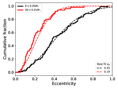
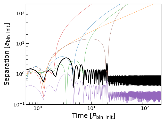
Figure 3: Results of scattering experiments. We populate binary systems (primary $0.7M_{\odot}$, secondary $M_{*}=0.3M_{\odot}$) with brown dwarfs that have the same total mass but different individual masses. The final binary e-distributions are Rayleigh in form (left panel, 100 cases each), with modes that depend only on the individual brown dwarf mass (eq. 3). The right panel shows an example case with the orbits of the brown dwarfs as colored curve, and the secondary as heavy black curve. The vertical axis is the distance to the binary centre of mass. All brown dwarfs are promptly ejected except for one that becomes bound to the primary.

Consider, at birth, the presence of one or more low-mass bodies (‘brown dwarfs’) in the binary system. Unless sheltered dynamically, they should be quickly ejected by the binary through close encounters. Such encounters tend to establish equi-partition of epicyclic energy among the bodies (Ida & Makino, 1992b),

$$e_{*}^{2}M_{*}\simeq e_{\rm BD}^{2}M_{\rm BD}\,,$$ (2)

where $M_{*}$ is the mass of the secondary. Setting $e_{\rm BD}\sim 1$ for ejection, we obtain,

$$e_{*}\simeq\left(\frac{M_{\rm BD}}{M_{*}}\right)^{1/2}\simeq 0.30\left(\frac{M_{\rm BD}}{0.03M_{\odot}}\right)^{1/2}\,\left(\frac{M_{*}}{0.3M_{\odot}}\right)^{-1/2}\,,$$ (3)

This expression does not depend on period, because the scattering dynamics is scale-free (ejection velocity is related to the local Keplerian velocity; also see Fig. 8 of Jurić & Tremaine, 2008). Moreover, if there is (even a weak) correlation between $M_{\rm BD}$ and $M_{*}$, this expression will also be insensitive to the stellar masses. Both insensitivities are what we observe in GAIA binaries.

We carry out numerical experiments (details in Appendix E) and present the results in Fig. 3. Each binary is endowed with a number of low-mass siblings. As the brown dwarfs are promptly cleared away, the binary eccentricities achieve a Rayleigh distribution, with the mode described roughly by eq. (2). To achieve the observed value of $\sigma_{e}=0.30$, we require $M_{\rm bd}\sim M_{*}/10$. We find that the outcome is not sensitive to the total number of brown dwarfs – in fact, as few as a couple brown dwarfs may suffice for the task (also see Ford & Rasio, 2008).

Could Nature provide such a set-up consistently? In the scenario of disk fragmentation, it is plausible that multiple low-mass objects would form alongside the dominant binary. At gravitational fragmentation, the characteristic mass is $\sim 10^{-2}M_{\odot}$ (e.g., Rafikov, 2005; Matzner & Levin, 2005; Xu et al., 2024). This is close to the above brown dwarf mass. Subsequent nonlinear evolution is currently unclear (Goodman & Tan, 2004; Levin, 2007). The fragments can accrete from the disk and/or merge with each other. They can also migrate due to disk torque. The prevalence of close binaries in nature suggests that, in many cases, some of these seeds can grow to reach the isolation mass ($\sim M_{\odot}$). At the same time, other small seeds may persist or may be continuously produced, as in the forming triple system observed by Tobin et al. (2016). If so, disk fragmentation sets the stage for later dynamical scattering.

Further investigations may reveal if $M_{\rm bd}/M_{*}$ does remain nearly constant in all disks. Moreover, if all close binaries have ejected at least one brown dwarf, this can explain all sub-stellar objects detected by imaging in young clusters and by microlensing surveys (Appendix F).

4 Conclusions

The GAIA mission greatly expands our sphere of vision. The number of AU-scale binaries, for which eccentricity information can be reliably extracted, rises from dozens to of order $10^{5}$. Among these, we select a largely un-biased sample of $\sim 3000$ systems to deduce the underlying eccentricity distribution. A simple and elegant Rayleigh distribution emerges, with a mode of $0.3$. The value of the mode appears invariant with respect to stellar mass and orbital period, but a more definitive conclusion will require careful study of the selection bias.

Such a distribution is almost certainly primordial in origin. Its (apparent) invariance points to a universal process. And the Rayleigh form itself suggests an origin in weak scatterings.

We hypothesize that, during the last phase of star formation, one or more brown dwarf siblings are ejected by the stellar binary. To reproduce the observed Rayleigh mode, the brown dwarf masses should be $\sim 1/10$ of the secondary masses. It is not known why this must be so. But if true, such brown dwarfs can account for almost all free-floating sub-stellar objects. Their kinematics may bear imprints of the ejection process.

It is natural to ask how far in period such a Rayleigh distribution extends. Based on current data, we speculate that it may reach tens of AU before it is fully replaced by a thermal distribution. GAIA DR4 should provide definitive answer on this question.

With this new discovery, the eccentricity distribution becomes a new marker for the process of disk fragmentation, joining rank with other measurables like period, metallicity, mass-ratio, and twin-fraction. It can be used to probe many interesting questions. For instance, do binaries in extreme environments (e.g., globular clusters, nuclear star clusters) form in disks? Does the Rayleigh mode vary with environmental factors? How do close-binaries pair and how does this pairing correlate with their eccentricities (Fig. 6)?

AU-scale binaries are important drivers for binary stellar evolution – given the AU-sizes of giant stars, these include most of the binaries that are destined to interact during their lifetimes, through tides, mass transfer and common envelope. The Rayleigh distribution, as opposed to the older uniform distribution, leads to fewer binary mergers. This new distribution should be adopted in synthetic studies of binary evolution.

We thank NSERC for research funding, and the GAIA collaboration for a marvelous gold mine.

Appendix A GAIA binary extraction

We construct a binary sample that is little affected by either detection bias or evolutionary changes.

Starting from the GAIA non-single-star catalog (Gaia Collaboration et al., 2023b), we apply a number of cuts consecutively. These steps and their resulting sample sizes are listed in Table 1. Our final sample (named the ‘gold’ sample) is homogeneous in primary properties (Sun-like dwarfs), and avoid any significant selection bias.

Here are some explanations. A fraction of the GAIA catalogue stars have determined astrophysical parameters. Among these, we retain only systems with main-sequence primaries, defined as

$$M_{G}>{\rm Max}\{4.0,\,\left[(B_{p}-R_{p})_{\rm de-red}-1\right]^{7}\}\,$$ (A1)

where $M_{G}$ is the absolute g-band magnitude and $(B_{p}-R_{p})_{\rm de-red}$ is the de-reddened color. We also remove those with ‘significance’ $<10$. Aside from producing a cleaner sample, this automatically rejects any binaries detected as ‘Eclipsing Binaries’. We exclude these binaries because many of them have eccentricities artificially set to zero.

We also select binaries with periods from $10^{2}-10^{3}$days. The former is set to avoid pollution from tidal circularization, while the latter is due to the finite coverage of GAIA DR3. To meaningfully compare against the detection completeness from mock pipelines (El-Badry et al., 2024), we proceed to retain only binaries characterized by astrometry (including ‘Orbital’ and ‘AstroSpectroSB1’ types). Among these, we require a further quality cut: ‘goodness-of-fit’ $<5$ if ‘phot-g-mean-mag $>13$, or $<10$ if otherwise. This filters out bad solutions, the threshold for which depends on brightness. A system is considered ‘Sun-like’ if the primary radius is within $[0.7,2.0]R_{\odot}$.

And lastly, for our ‘gold’ sample, we set a maximum distance of $150$pc. This last cut leaves us with $\sim 3000$ systems, a tiny fraction of the original data($\leq 1\%$). About $\sim 45\%$ of the ‘gold’ sample have only astrometric orbits (‘Orbital’), while the rest are additionally characterized by radial velocity (‘AstroSpectroSB1’). The latter group tend to be brighter.

Ideally, we would also like to remove systems with white-dwarf secondaries. Their eccentricities have likely been strongly suppressed during the giant phase. However, doing this thoroughly is difficult at the moment (Shahaf et al., 2023). Fortunately, such binaries mostly contribute at the longest periods. Results in Fig. 2 show that their impact is likely minor.

Regardless of the cut, all samples exhibit e-distributions that have a Rayleigh shape. Their Rayleigh modes, however, differ (Table 1). Most cuts return a lower mode ($\sigma_{e}\sim 0.25$), except for the ‘gold’ sample ($\sigma_{e}\sim 0.30$). Such a difference, we argue (Fig. 2), reflects not intrinsic variation, but impact of the selection bias (Appendix B).

Appendix B Characterizing the Detection Bias

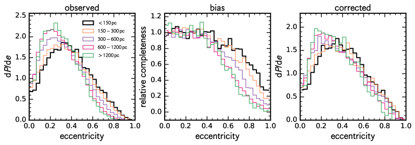
Figure 4: Correction for detection bias. The left panel repeats that in Fig. 1. The middle panel shows the completeness as a function of binary eccentricity, obtained from the mock astrometry pipeline (El-Badry et al., 2024). The right panel shows the corrected values. Correction brings the different distributions into better agreements with each other, though some differences still exist.

Gaia is, generically, less sensitive to high-eccentricity orbits. High-eccentricity binaries spend more time near apoapse and are thus less likely to have their orbits well sampled by Gaia observations, which occur at quasi-random times. This results in orbits that are on average less well constrained at high eccentricity, and less likely to pass the stringent quality cuts imposed on the orbital solutions published in Gaia DR3. Such a bias very likely affects both astrometric and RV orbits, but it has thus far been quantitatively modeled only for astrometric orbits, and for this reason we focus on astrometric orbits in this work.

We use the forward-model of Gaia astrometric orbit catalogs described by El-Badry et al. (2024) to quantify the eccentricity bias in our sample. The model produces realistic epoch astrometry for each simulated binary and fits it using the same cascade of astrometric models used in producing the DR3 binary catalogs (see Halbwachs et al., 2023). Following El-Badry et al. (2024), we generate a realistic population of binaries within 2 kpc of the Sun, mock-observe them, and produce a mock catalog. Unlike El-Badry et al. (2024), who assumed an eccentricity distribution following Moe & Di Stefano (2017), we adopt a uniform eccentricity distribution, which allows us to trace Gaia’s eccentricity bias. Other properties of the simulated binaries (e.g. masses, ages, evolutionary states, orbital periods, 3D locations in the Galaxy) are chosen as described by El-Badry et al. (2024) and are reasonably good approximations of reality. To represent the bias specific to the observational sample analyzed here, we exclude binaries containing red giants and require astrometric significance $>10$ in addition to the quality cuts imposed on the solutions published in DR3.

The results of these simulations are shown in the middle panel of Figure 4. As with the observed data, we show individual distance bins separately. We normalize the distributions in each eccentricity bin such that the average relative completeness at $0<e<0.3$ is unity. A bias against high eccentricities exists in all distance bins, but it is more severe at large distances, where orbits have smaller angular size at fixed period and thus lower astrometric SNR. This trend mirrors what is found in the observed sample. The simulations suggest that Gaia sample with $d<150$ pc is largely unbiased at $e<0.5$, but a bias against high eccentricities is present at higher eccentricities. At $e>0.9$, the completeness is $\approx 3$ times lower than at $e<0.5$.

The right panel of Figure 4 shows the normalized eccentricity distribution of the observed samples after correcting for incompleteness. The corrected eccentricity distributions in different distance bins are in better agreement with one another, although some trend of lower eccentricity at larger distances is still present. This could reflect imperfections in the forward-model, although it could also be a result of a mass-dependent eccentricity distribution, since more distant binaries are on average brighter and more massive.

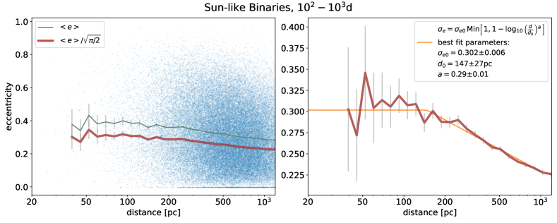
Figure 5: We use the ‘Sun-like’ sample in Table 1 to explore the effects of detection bias. The left panel shows that the mean eccentricity ($\langle e\rangle$) gradually declines with distance. The brown line is $\langle e\rangle/\sqrt{\pi/2}$, a proxy for the Rayleigh mode. Using equation B1 to describe how distance affects the mode, we find an an intrinsic Rayleigh mode of $\sigma_{e0}\approx 0.30$, and that systems inward of $d_{0}\sim 150$pc should be free of detection bias.

We also use the observed sample itself to gauge how much this bias affects the measurement for the Rayleigh mode. This is independent of the above mock pipeline and serves as a self-calibration.

In Fig. 5, we present the eccentricities and their mean values ($\langle e\rangle$) as functions of distance from Earth. We use $\langle e\rangle/\sqrt{\pi/2}$ as a proxy for the Rayleigh mode $\sigma_{e}$ and fit the following data-inspired form,

$$\sigma_{e}(d)=\sigma_{e0}\,{\rm Min}\left[1,1-\log_{\rm 10}\left(\frac{d}{d_{0}}\right)^{a}\right]\,.$$ (B1)

where $\sigma_{e0}$ is the intrinsic Rayleigh mode. Such a form asserts that, for systems closer than $d_{0}$, $\sigma_{e}=\sigma_{e0}$, i.e., there is little bias for the bulk of the Rayleigh distribution (but there can still be bias at high eccentricities). Such a form is reasonable for a Rayleigh distribution (which concentrates at low-e), but is less so for a, e.g., power-law distribution.

The observed data yields the following best-fit parameters: $\sigma_{e0}=0.301\pm 0.006$, $d_{0}=147\pm 27$pc, and $a=0.29\pm 0.01$. This validates our main results, that the primordial Rayleigh scale is $\sigma_{e}\sim 0.30$, as measured from the ‘gold’ sample. This does not mean, however, that the ‘gold’ sample is complete to $d_{0}\sim 150$pc – it is not. It is missing binaries of high eccentricities (see Fig. 4), as well as binaries of comparable brightnesses, or those with very low-mass secondaries.

Appendix C Dependence on Binary Mass Ratio?

Whether the Rayleigh mode depends on the mass-ratio in a binary is of high relevance for its origin. So we conduct a preliminary analysis, using a subset of the GAIA sample where both stellar masses are reported. Our conclusion is ambiguous.

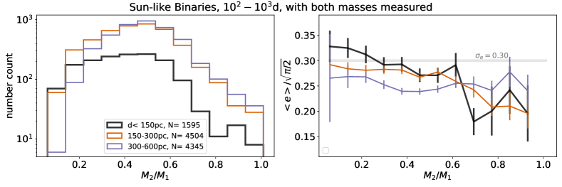
Figure 6: A possible dependence of the Rayleigh mode on binary mass-ratios is seen, in the ‘Sun-like’ sample. The left panel shows the number of systems with reported mass-ratios, divided by distances. The drop-off towards equal masses may be explained by astrometric bias. The right panel shows the proxy for the Rayleigh mode, $\langle e\rangle/\sqrt{\pi/2}$. A possible reduction towards equal-mass is seen, but we remain suspicious.

We divide the ‘Sun-like’ sample by distances, as in Fig. 1 and plot their properties in relation to the mass-ratio. Only the closest three groups have enough cases for statistics. Fig. 6 shows that the binary counts drop off steeply towards equal-mass, in contrast to that found in the spectroscopic sample by Moe & Di Stefano (2017). This is explained, at least partly, by the fact that an equal-brightness binary exhibits zero astrometric signal. We use mean eccentricity as a proxy for the Rayleigh mode and find that it also drops off towards equal masses. While this seems statistically significant, Moreover, it occurs at the same mass ratio as the number drop-off, suggesting a common origin in detection bias. A more detailed analysis is required to establish the authenticity of this result.

Appendix D The unimportance of stellar encounters

Could the AU-scale binaries have obtained their eccentricities by scattering passing stars, especially while they are still within their birth clusters?

We hold that this is unlikely. We present multiple arguments.

For our AU-binaries, we are in the ‘hard’ binary case (Heggie, 1975), where the binary orbital velocity ($V_{\rm orb}$) exceeds the mean dispersion velocity of the cluster ($V_{\infty}$, e.g, $V_{\infty}\sim 12$ km/s in the dense core of 47 Tuc). If we consider impacts with the closet approach distance $R_{\rm min}\geq a$ (binary separation), the encounter is in the adiabatic limit where the binary have time to revolve multiple times during one close-approach of the third star. Moreover, the third star orbit is close to being parabolic. An initially circular binary will receive a kick in eccentricity that is of order (Heggie & Rasio, 1996; Spurzem et al., 2009),

$$\delta e \approx 3\sqrt{2\pi}\frac{M_{3}M_{12}^{1/4}}{M_{123}^{5/4}}\left(\frac{2R_{\rm min}}{a}\right)^{3/4}\,$$ (D1)

$$\times\exp\left[-{2\over 3}\left(\frac{2M_{12}}{M_{123}}\right)^{1/2}\left(\frac{R_{\rm min}}{a}\right)^{3/2}\right]\,,$$

where the total binary mass $M_{12}=M_{1}+M_{2}$, and $M_{123}=M_{1}+M_{2}+M_{3}$ with $M_{3}$ being the perturber mass. For $V_{\rm min}=\sqrt{GM_{12}/R_{\rm min}}\gg V_{\infty}$, the impact parameter is of order $b\approx R_{\rm min}V_{\rm min}/V_{\infty}$ (or else $b\sim R_{\rm min}$). We adopt the set of masses, $M_{i}=[1.0,0.7,0.3]$ and find $R_{\rm min}\sim 2a$, if one requires a kick magnitude $\delta e=0.3$. The adiabatic limit brings about an exponential suppression of the kick. This means we need only to account for the one encounter that has the closest impact parameter. All other encounters do not add substantially.

Consider a cluster with total mass $M_{\rm c}$ and size $R_{\rm c}$, $V_{\infty}\sim\sqrt{GM_{c}/R_{c}}$, number density of stars $N_{c}=M_{\rm c}/M_{*}/\pi R_{c}^{3}$. The mean-free-time to have an impact such that $R_{\rm min}\sim 2a$ is

$$t \sim \frac{1}{n(\pi b^{2})V_{\infty}}\sim 4\times 10^{8}{\rm yrs}\left(\frac{N_{c}}{10^{5}/{\rm pc}^{3}}\right)^{-1}\left(\frac{V_{\infty}}{10\,\rm km/\,\rm s}\right)\,$$ (D2)

$$\times\left(\frac{M_{12}}{1.7M_{\odot}}\right)^{-1}\left(\frac{a}{1{\rm AU}}\right)^{-1}\,.$$

where we have scaled the cluster density and velocity by values appropriate for a very dense region, the core of 47 Tuc (McLaughlin et al., 2006). Most stars are formed in much less dense clusters that dissolves in tens to hundreds of million years. Outside these birth clusters, the density is much lower and the impact is even smaller. So overall, AU-scale binaries are unlikely to have been affected by passing-by stars (Parker et al., 2009).

Even if the above estimate is wrong, we argue that an origin in stellar scattering can be excluded. First, scattering tends to affect the wider binaries more, while the observed Rayleigh mode is largely invariant with the orbital period. Second, if stellar scattering is so strong as to produce $e\sim 0.3$ for AU-scale binaries, it would also have dissolved all binaries that are a few times wider (Heggie, 1975; Spurzem et al., 2009).

Appendix E Numerical Simulations of Brown Dwarf Ejections

We simulate the gravitational interactions between stellar binary and multiple brown dwarfs, with a focus on the effects on binary eccentricity.

The binary is composed of a $0.7M_{\odot}$ primary and a $0.3M_{\odot}$ secondary. They are initialized with a circular orbit with $a=a_{\rm bin,init}=1$AU. A crowd ($N_{\rm bd}$) of brown dwarfs each with mass $M_{\rm bd}$ is uniformly sprinkled in logarithmic distance (from $0.03a_{\rm bin,init}$ to $0.9a_{\rm bin,init}$) between the binary stars. All initial orbital angles are drawn randomly. The initial eccentricities are zero, and the mutual inclinations are drawn from a Rayleigh distribution with $\sigma_{i}=10^{-3}$rad. We ignore collisions by setting all physical sizes of the particles to zero. We integrate the system using the IAS15 integrator in REBOUND (Rein & Liu, 2012; Rein & Spiegel, 2015).

We carry out 100 simulations for each of the following two sets of parameters: $N_{\rm bd}=6$, $M_{\rm bd}=0.05M_{\odot}$; $N_{\rm bd}=30$, $M_{\rm bd}=0.01M_{\odot}$. The dynamics are similar. Within a short time (typically tens of orbits), most of the brown dwarfs have been ejected. The remaining couple may become bound to one or the other stars. During these ejections, the initial conditions are quickly erased, and we observe that the binaries are hardened and become eccentric. The binary e-distribution is Rayleigh in form, with best-fit modes $\sigma_{e}=0.19$ and $0.35$, for the two cases respectively. The binary inclinations are also disturbed from the original plane.

The Rayleigh mode is sensitive only to the individual brown dwarf mass, as indicated by eq. (2). The number of brown dwarfs is not relevant. In fact, even scattering as few as one brown dwarf may be sufficient to achieve the same e-distribution, as is observed in the 2-planet scattering experiments of Ford & Rasio (2008).

Our experiments do not account for mergers. This is reasonable, as dynamical ejection occurs too fast to allow very close encounters.

Appendix F Enough free-floating Brown Dwarfs?

If close binaries acquire their eccentricities by ejecting brown dwarfs, one expects to see those ejected bodies.

We crudely estimate their contributions to the Galactic mass function, for two limiting cases. In the first case (‘excitation’) we allow one brown dwarf per system, enough to excite the observed eccentricity. In the second case (‘hardening’) we assume that all close binaries were originally wide, but scatter enough brown dwarfs to wind up at their current separations.

Solar-type binaries in the field follow a log-normal distribution in orbital periods (Duquennoy & Mayor, 1991; Raghavan et al., 2010; Moe et al., 2019).

$${{df_{\rm binary}}\over{d\log P}}\approx{{f_{\rm binary}}\over{\sqrt{2\pi}\sigma_{\log P}}}\,\exp\left[-{1\over 2}\left(\frac{\log P-\log P_{0}}{\sigma_{\log P}}\right)^{2}\right]$$ (F1)

with the total binary fraction $f_{\rm binary}\sim 0.50$, $\log P_{0}\sim 5$ (or $\sim 40$au), and $\sigma_{\log P}\sim 2.3$. Here, all logarithms are 10-based, and all periods are in unit of days. We adopt $M_{1}\sim 1M_{\odot}$ and a companion mass of $M_{2}\sim 0.5M_{\odot}$.

For ‘excitation’, the total mass of ejected bodies relative to that in all Sun-like stars (binary and single) is

$$f_{\rm excitation} \equiv {{\displaystyle\sum_{\rm binary}M_{\rm bd}}\over{\displaystyle\sum_{\rm single}M_{1}+\displaystyle\sum_{\rm binary}(M_{1}+M_{2})}}$$ (F2)

$$\approx {1\over 10}{{M_{2}}\over{M_{1}}}\int^{P_{0}}_{P=10d}{{df_{\rm binary}}\over{d\log P}}d\log P\,$$

$$\approx\, 0.01\,,$$

where we have adopted $M_{\rm bd}\sim M_{2}/10$ (eq. 3) and included all binaries from $10$d to $P_{0}=10^{5}$d.

To harden binaries from an initial separation $a_{0}$ to a new separation $a\ll a_{0}$, the amount of mass ejected (with parabolic orbits) is $M_{\rm ejected}\sim\ln(a_{0}/a)\,M_{2}\sim 2/3\ln(P_{0}/P)\,M_{2}$. Integrating over the same period range yields

$$f_{\rm hardening} \equiv {{\displaystyle\sum_{\rm binary}M_{\rm bd}}\over{\displaystyle\sum_{\rm single}M_{1}+\displaystyle\sum_{\rm binary}(M_{1}+M_{2})}}$$ (F3)

$$\approx {2\over 3}{{M_{2}}\over{M_{1}}}\int^{P_{0}}_{P=10d}{{df_{\rm binary}}\over{d\log P}}\times(\ln P_{0}-\ln P)\,d\log P$$

$$\approx 0.30\,.$$

What are the observational constraints? In the following, we compile the stellar/sub-stellar mass functions using two different types of studies: those that count objects in young stellar clusters, and those that employ microlensing.

Using data from Pleides (120 Myrs old), Moraux et al. (2003) showed that the mass function at the low end can be well fit by a log-normal distribution (their eq. 3). In even younger clusters ($\sigma$ Ori at 3 Myrs, Upper Sco at 5-10 Myrs), there appears to be more free-floating objects than described by this log-normal form: for masses below $\sim 0.05M_{\odot}$ (Lodieu, 2013; Béjar et al., 2011) found a mass-function that roughly goes as $dN/d\log M\propto M^{0}$. So we append a flat tail to the above log-normal distribution. For the microlensing data, we adopt solution CR1 in Sumi et al. (2023), inferred using lensing events from the Galactic bulge. These two mass functions differ in form (left panel of Fig. 7), but they give roughly the same values in cumulative mass (right panel).

We find that in the sub-stellar regime that is of interest to us, the mass function is top-heavy. Moreover, the mass in the relevant brown dwarf range ($M_{\rm bd}\sim 0.05M_{\odot}$) is of order $2\%$ of the stellar mass. This means there are enough brown dwarfs to excite binary eccentricity, but far too few to account for binary hardening.

This mass comparison suggests that, if the ejection scenario is correct, almost all brown dwarfs should be formed in massive disks, as companions to stellar binaries.

An interesting prediction for such a scenario is that the ejection event may leave evidence in the kinematics of these bodies. They should be leaving their birth systems with a velocity dispersion that is of order the orbital escape velocity. This is a worthy topic for further study.

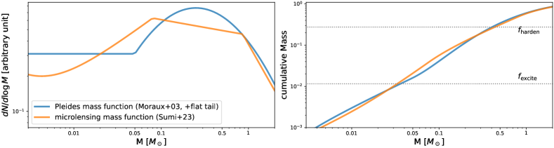
Figure 7: Mass functions in the low-mass end, in differential (left panel) and cumulative forms (right panel). The two determinations are from young clusters and from microlensing of bulge stars. For both cases, the cumulative mass below $0.05M_{\odot}$ is about $2\%$, enough to excite Solar-type close binaries ($f_{\rm excite}$), but not enough to harden them ($f_{\rm harden}$).

Appendix G Is there only a single Rayleigh?

We have obtained a best-fit Rayleigh of $\sigma_{e}=0.30$ for our ’gold’ sample. But given the large sample size ($N=3071$), it is possible to extract more information. We query the data to determine if it prefers other solutions, in particular, two separate Rayleigh distributions that may arise when there are two different physical processes at play.

In the following, we employ a Bayesian framework to answer this question. The marginal likelihood, or evidence, that data $D$ are generated by a model $\mathcal{M}$, is given by the integral

$$\mathcal{E}(D|\mathcal{M})=\int\mathrm{Pr}(\boldsymbol{\theta}|\mathcal{M})\mathrm{Pr}(D|\boldsymbol{\theta},\mathcal{M})d\boldsymbol{\theta}.$$ (G1)

The ratio between marginal likelihoods for two different models then gives a Bayes factor that provides one metric for how much more (or less) strongly a given model is supported by the data. In our case the data $D$ are binary eccentricities in the ‘gold’ sample. For a given data set $D=\{e_{1},...,e_{i},...,e_{N}\}$ we incorporate observational uncertainty by writing $\mathrm{Pr}(D|\boldsymbol{\theta},\mathcal{M})=\prod_{i=1}^{N}\int\mathrm{Pr}(e_{i}|e_{\textrm{true}})\mathrm{Pr}(e_{\textrm{true}}|\boldsymbol{\theta},\mathcal{M})\text{d}e_{\textrm{true}},$ where we adopt $\mathrm{Pr}(e_{i}|e_{\textrm{true}})$ to be a truncated Gaussian distribution with a standard deviation of $0.025$.

G.1 Single Rayleigh

Model $\mathcal{M}_{1}$ assumes that the eccentricities of the entire population are distributed according to a single Rayleigh distribution,

$$\mathrm{Pr}(D|\boldsymbol{\theta}_{e},\mathcal{M}_{1}) = \prod_{i=1}^{N}\frac{e_{i}}{\sigma_{e}^{2}}\exp\left(-\frac{e_{i}^{2}}{2\sigma_{e}^{2}}\right)$$ (G2)

$$= \sigma_{e}^{-2N}\mathcal{P}\exp\left(-\frac{S}{2\sigma_{e}^{2}}\right)\,,$$

where $\mathcal{P}=\prod_{i}^{N}e_{i},$ and $S=\sum_{i}^{N}e_{i}^{2}.$ For a uniform probability distribution $\mathrm{Pr}(\sigma_{e}|\mathcal{M}_{1})=(\Delta\sigma)^{-1}$, where $\Delta\sigma=\sigma_{\textrm{max}}-\sigma_{\textrm{min}}$ for $\sigma_{\mathrm{min}}\leq\sigma_{e}\leq\sigma_{\mathrm{max}}$, the evidence is then given (in the absence of observational uncertainty) as

$$\mathcal{E}(D|\mathcal{M}_{1})=(\Delta\sigma)^{-1}\int_{\sigma_{\mathrm{min}}}^{\sigma_{\mathrm{max}}}\mathcal{P}\sigma_{e}^{-2N}\exp\left(-\frac{S}{2\sigma_{e}^{2}}\right)d\sigma_{e}$$ (G3)

$$=(\Delta\sigma)^{-1}2^{N-3/2}S^{1/2-N}\mathcal{P}\Gamma\left(N-1/2,\frac{S}{2\sigma_{e}^{2}}\right)\Bigg{|}^{\sigma_{\mathrm{max}}}_{\sigma_{\mathrm{min}}}\,,$$

where $\Gamma$ is the incomplete Gamma function. We find that, for our ‘gold’ sample, the likelihood $\textrm{Pr}(D_{\textrm{Gaia}}|\sigma_{e},\mathcal{M})$ approaches a singularly peaked function at $\sigma_{e}=0.30$. So $\mathcal{E}(D_{\textrm{Gaia}}|\mathcal{M}_{1})\gg 1$ for any choices of $\sigma_{\textrm{max}}$ and $\sigma_{\textrm{min}}$, regardless of the observational uncertainties.

G.2 Double Rayleigh?

Can the GAIA sample be instead drawn from two separate Rayleigh distributions? We consider a mixture model $\mathcal{M}_{2}$ with

$$\mathrm{Pr}(D|\sigma_{1},\sigma_{2},f,\mathcal{M}_{2}) = \prod_{i=1}^{N}\left[f\dfrac{e_{i}}{\sigma_{1}^{2}}\exp\left(-\dfrac{e_{i}^{2}}{2\sigma_{1}^{2}}\right)\right.$$ (G4)

$$\left.+(1-f)\dfrac{e_{i}}{\sigma_{2}^{2}}\exp\left(-\dfrac{e_{i}^{2}}{2\sigma_{2}^{2}}\right)\right],$$

where $0\leq f\leq 1.$ Assuming $\textrm{Pr}(\sigma_{1},\sigma_{2},f|\mathcal{M}_{2})=1/(\Delta\sigma)^{2}$, we compute the evidence $\mathcal{E}(D_{\textrm{Gaia}}|\mathcal{M}_{2})$ numerically (using Clenshaw-Curtis quadratures). For like values of $\sigma_{\textrm{max}}$ and $\sigma_{\textrm{min}},$ we find $\mathcal{E}(D_{\textrm{Gaia}}|\mathcal{M}_{1})/\mathcal{E}(D_{\textrm{Gaia}}|\mathcal{M}_{2})\sim 2-5$ when $\sigma_{\textrm{min}}\gtrsim 0.1$ and $\sigma_{\textrm{max}}>0.303.$ This does not provide particularly strong support for a single Rayleigh distribution over a double one. However, for any intermediate mixing fraction $0<f<1$, we find that the likelihood $\mathcal{L}=\textrm{Pr}(D_{\textrm{Gaia}}|\sigma_{1},\sigma_{2},f,\mathcal{M}_{2})$ peaks at $\sigma_{1}\approx\sigma_{2}\approx 0.303$, which simply corresponds to a single Rayleigh distribution with the same mode; the flexibility of the mixture model provides no added utility.

When $\sigma_{\textrm{min}}\lesssim 0.05$, the Gaia data provide a stronger evidence for a double Rayleigh model with $\sigma_{1}=0.303,$ $\sigma_{2}\ll 1$, and $1-f\ll 1$ (i.e., mostly the primary Rayleigh mode $\sigma_{1}=0.303$). However, we discount this model for two reasons. First, it amounts to an over-fit of the small eccentricity data. Second, there is a strange (but small) excess of $e=0$ points in the data (as seen in the left panel of Fig. 5) that likely reflects issues in the GAIA pipeline.

Appendix H Binaries at Longer Periods?

In the following, we ask whether the same Rayleigh distribution extends to binaries outside $10^{3}$d.

Knowing that wide binaries have thermal distributions (Tokovinin, 2020; Hwang et al., 2021), we can imagine at least two possibilities: the Rayleigh may persist but with an increasing mode further out, smoothly connecting up to the thermal distribution; or both distributions co-exist, with the fraction of Rayleigh (with the same mode) gradually going down to zero. Given the invariance of the Rayleigh mode in our ‘gold’ sample, we choose to focus on the second possibility. We draw some partial conclusions based on two different samples.

The first is the previous ground-based sample from Raghavan et al. (2010), which includes $58$ binaries in the period range $10^{3}-10^{5}$d (or $\sim 2-40$AU). We consider a model $\mathcal{M}_{3}$ in which the eccentricities are distributed according to a mixture of Rayleigh and thermal:

$$\mathrm{Pr}(D|\sigma_{e},f,\mathcal{M}_{3})=\prod_{i=1}^{N}\left[f\dfrac{e_{i}}{\sigma_{e}^{2}}\exp\left(-\dfrac{e_{i}^{2}}{2\sigma_{e}^{2}}\right)+2(1-f)e_{i}\right]\,,$$ (H1)

with $f$ being the Rayleigh fraction. We adopt a flat prior for $f$ and a prior $\mathrm{Pr}(\sigma_{e}|\mathcal{M}_{3})=\delta(\sigma_{e}-0.303),$ which equates to conditioning based on the knowledge gained from our Gaia sample.

We then compute the evidence $\mathcal{E}_{\textrm{mix}}=\mathcal{E}(D_{\textrm{LP}}|\mathcal{M}_{3})$ for the long-period sample. Our results indicate that a mixture fraction of $f=0.52$ best describes the data. Comparing against evidence values computed for a purely thermal, a purely uniform ($\mathcal{E}_{\textrm{therm}}=2^{N}\mathcal{P}$ and $\mathcal{E}_{\textrm{uni}}=1$, respectively), and a purely Rayleigh distributions, we find Bayes factors $\mathcal{E}_{\textrm{mix}}/\mathcal{E}_{\textrm{therm}}\approx 6.5\times 10^{3}$, $\mathcal{E}_{\textrm{mix}}/\mathcal{E}_{\textrm{uni}}\approx 12.3$, and $\mathcal{E}_{\textrm{mix}}/\mathcal{E}(D_{\textrm{LP}}|\mathcal{M}_{1})\approx 20.2.$ These factors indicate that the mixture model $\mathcal{M}_{3}$ is much better supported by the long-period data than a thermal eccentricity distribution, and marginally better supported than a uniform or a Rayleigh distribution. These results are graphically displayed in Fig. 8.

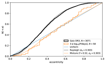
Figure 8: The cumulative histogram of eccentricity distribution for the long-period ($10^{3}-10^{5}$d) binary sample from Raghavan et al. (2010); Moe & Di Stefano (2017). It best supports a model that is a mixture of a Rayleigh and a thermal distribution (smooth orange curve). The other curves show the variety of models we compare against (thermal, uniform, and pure Rayleigh).

The second sample we consider comes from resolved GAIA binaries (El-Badry et al., 2021). Hwang et al. (2022) established, statistically, an eccentricity distribution by measuring the instantaneous velocity-position ($v-r$) angles that are projected on the sky (see also Tokovinin, 2020). Their results are shown in Fig. 9 for binaries with projected separations that fall within $10-1000$AU. In the absence of a better model, they parameterized the eccentricity distribution as a power-law, $dN/de\propto e^{\eta}$ and found that the value of $\eta$ rises from 0 (‘uniform’) at $\sim 50$ au, to $1$ (‘thermal’) at $\sim 500$au, and $>1$ (‘super-thermal’) beyond. Alternatively, as we show in Fig. 9, the so-called ‘uniform’ distribution can easily be swapped for our above mixture model. The data quality is not sufficient to tell the two apart.

These two pieces of evidence, taken together, suggest that the Rayleigh distribution may persist to at least tens of AU, and the apparent change in $\eta$ with period (Hwang et al., 2022) may simply reflect the decreasing fraction of the Rayleigh with increasing period.

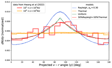
Figure 9: Distribution in the sky-projected displacement-velocity angle $\gamma$ for resolved binaries. The observed values (thick histograms for different values of projected separation $s$) are adopted from Fig. 6 of Hwang et al. (2022), and different models are in thin lines, with our best-fit mixture model (§G) in red. Wide binaries ($10^{2}<s<10^{3}$au) are best described by a thermal distribution, but close binaries ($10^{1}<s<10^{2}$au) can be described equally well by a uniform distribution ($dN/de={\rm const}$) or by our mixture model.

References

- Béjar et al. (2011) Béjar, V. J. S., Zapatero Osorio, M. R., Rebolo, R., et al. 2011, ApJ, 743, 64, doi: 10.1088/0004-637X/743/1/64
- Duchêne & Kraus (2013) Duchêne, G., & Kraus, A. 2013, ARA&A, 51, 269, doi: 10.1146/annurev-astro-081710-102602
- Duquennoy & Mayor (1991) Duquennoy, A., & Mayor, M. 1991, A&Ap, 248, 485
- El-Badry et al. (2024) El-Badry, K., Lam, C., Holl, B., et al. 2024, arXiv e-prints, arXiv:2411.00088. https://arxiv.org/abs/2411.00088
- El-Badry & Rix (2019) El-Badry, K., & Rix, H.-W. 2019, Monthly Notices of the Royal Astronomical Society: Letters, 482, L139
- El-Badry et al. (2021) El-Badry, K., Rix, H.-W., & Heintz, T. M. 2021, MNRAS, 506, 2269, doi: 10.1093/mnras/stab323
- El-Badry et al. (2019) El-Badry, K., Rix, H.-W., Tian, H., Duchêne, G., & Moe, M. 2019, MNRAS, 489, 5822, doi: 10.1093/mnras/stz2480
- Fischer & Marcy (1992) Fischer, D. A., & Marcy, G. W. 1992, ApJ, 396, 178, doi: 10.1086/171708
- Ford & Rasio (2008) Ford, E. B., & Rasio, F. A. 2008, ApJ, 686, 621, doi: 10.1086/590926
- Gaia Collaboration et al. (2016) Gaia Collaboration, Prusti, T., de Bruijne, J. H. J., et al. 2016, A&Ap, 595, A1, doi: 10.1051/0004-6361/201629272
- Gaia Collaboration et al. (2023a) Gaia Collaboration, Vallenari, A., Brown, A. G. A., et al. 2023a, A&Ap, 674, A1, doi: 10.1051/0004-6361/202243940
- Gaia Collaboration et al. (2023b) Gaia Collaboration, Arenou, F., Babusiaux, C., et al. 2023b, A&Ap, 674, A34, doi: 10.1051/0004-6361/202243782
- Geller & Mathieu (2012) Geller, A. M., & Mathieu, R. D. 2012, AJ, 144, 54, doi: 10.1088/0004-6256/144/2/54
- Geller et al. (2021) Geller, A. M., Mathieu, R. D., Latham, D. W., et al. 2021, AJ, 161, 190, doi: 10.3847/1538-3881/abdd23
- Goodman & Tan (2004) Goodman, J., & Tan, J. C. 2004, ApJ, 608, 108, doi: 10.1086/386360
- Greenzweig & Lissauer (1992) Greenzweig, Y., & Lissauer, J. J. 1992, Icarus, 100, 440, doi: 10.1016/0019-1035(92)90110-S
- Halbwachs et al. (2023) Halbwachs, J.-L., Pourbaix, D., Arenou, F., et al. 2023, A&Ap, 674, A9, doi: 10.1051/0004-6361/202243969
- Heggie (1975) Heggie, D. C. 1975, MNRAS, 173, 729, doi: 10.1093/mnras/173.3.729
- Heggie & Rasio (1996) Heggie, D. C., & Rasio, F. A. 1996, MNRAS, 282, 1064, doi: 10.1093/mnras/282.3.1064
- Hwang et al. (2021) Hwang, H.-C., Ting, Y.-S., Schlaufman, K. C., Zakamska, N. L., & Wyse, R. F. G. 2021, MNRAS, 501, 4329, doi: 10.1093/mnras/staa3854
- Hwang et al. (2022) Hwang, H.-C., Ting, Y.-S., & Zakamska, N. L. 2022, MNRAS, 512, 3383, doi: 10.1093/mnras/stac675
- Ida & Makino (1992a) Ida, S., & Makino, J. 1992a, Icarus, 96, 107, doi: 10.1016/0019-1035(92)90008-U
- Ida & Makino (1992b) —. 1992b, Icarus, 98, 28, doi: 10.1016/0019-1035(92)90203-J
- Jeans (1919) Jeans, J. H. 1919, MNRAS, 79, 408, doi: 10.1093/mnras/79.6.408
- Jurić & Tremaine (2008) Jurić, M., & Tremaine, S. 2008, ApJ, 686, 603, doi: 10.1086/590047
- Kratter & Lodato (2016) Kratter, K., & Lodato, G. 2016, ARA&A, 54, 271, doi: 10.1146/annurev-astro-081915-023307
- Kratter et al. (2010) Kratter, K. M., Matzner, C. D., Krumholz, M. R., & Klein, R. I. 2010, ApJ, 708, 1585, doi: 10.1088/0004-637X/708/2/1585
- Levin (2007) Levin, Y. 2007, MNRAS, 374, 515, doi: 10.1111/j.1365-2966.2006.11155.x
- Lodieu (2013) Lodieu, N. 2013, MNRAS, 431, 3222, doi: 10.1093/mnras/stt402
- Malhotra & Wang (2017) Malhotra, R., & Wang, X. 2017, MNRAS, 465, 4381, doi: 10.1093/mnras/stw3009
- Matzner & Levin (2005) Matzner, C. D., & Levin, Y. 2005, ApJ, 628, 817, doi: 10.1086/430813
- McLaughlin et al. (2006) McLaughlin, D. E., Anderson, J., Meylan, G., et al. 2006, ApJS, 166, 249, doi: 10.1086/505692
- Moe & Di Stefano (2017) Moe, M., & Di Stefano, R. 2017, ApJS, 230, 15, doi: 10.3847/1538-4365/aa6fb6
- Moe et al. (2019) Moe, M., Kratter, K. M., & Badenes, C. 2019, ApJ, 875, 61, doi: 10.3847/1538-4357/ab0d88
- Moraux et al. (2003) Moraux, E., Bouvier, J., Stauffer, J. R., & Cuillandre, J. C. 2003, A&Ap, 400, 891, doi: 10.1051/0004-6361:20021903
- Offner et al. (2023) Offner, S. S. R., Moe, M., Kratter, K. M., et al. 2023, in Astronomical Society of the Pacific Conference Series, Vol. 534, Protostars and Planets VII, ed. S. Inutsuka, Y. Aikawa, T. Muto, K. Tomida, & M. Tamura, 275, doi: 10.48550/arXiv.2203.10066
- Parker et al. (2009) Parker, R. J., Goodwin, S. P., Kroupa, P., & Kouwenhoven, M. B. N. 2009, MNRAS, 397, 1577, doi: 10.1111/j.1365-2966.2009.15032.x
- Rafikov (2005) Rafikov, R. R. 2005, ApJL, 621, L69, doi: 10.1086/428899
- Raghavan et al. (2010) Raghavan, D., McAlister, H. A., Henry, T. J., et al. 2010, ApJS, 190, 1, doi: 10.1088/0067-0049/190/1/1
- Rein & Liu (2012) Rein, H., & Liu, S. F. 2012, A&Ap, 537, A128, doi: 10.1051/0004-6361/201118085
- Rein & Spiegel (2015) Rein, H., & Spiegel, D. S. 2015, MNRAS, 446, 1424, doi: 10.1093/mnras/stu2164
- Shahaf et al. (2023) Shahaf, S., Bashi, D., Mazeh, T., et al. 2023, MNRAS, 518, 2991, doi: 10.1093/mnras/stac3290
- Spurzem et al. (2009) Spurzem, R., Giersz, M., Heggie, D. C., & Lin, D. N. C. 2009, ApJ, 697, 458, doi: 10.1088/0004-637X/697/1/458
- Sumi et al. (2023) Sumi, T., Koshimoto, N., Bennett, D. P., et al. 2023, AJ, 166, 108, doi: 10.3847/1538-3881/ace688
- Tobin et al. (2016) Tobin, J. J., Kratter, K. M., Persson, M. V., et al. 2016, Nature, 538, 483, doi: 10.1038/nature20094
- Tobin et al. (2020) Tobin, J. J., Sheehan, P. D., Megeath, S. T., et al. 2020, ApJ, 890, 130, doi: 10.3847/1538-4357/ab6f64
- Tokovinin (2020) Tokovinin, A. 2020, MNRAS, 496, 987, doi: 10.1093/mnras/staa1639
- Tokovinin (2000) Tokovinin, A. A. 2000, A&Ap, 360, 997
- Tremaine (2015) Tremaine, S. 2015, ApJ, 807, 157, doi: 10.1088/0004-637X/807/2/157
- Xu et al. (2024) Xu, W., Jiang, Y.-F., Kunz, M. W., & Stone, J. M. 2024, arXiv e-prints, arXiv:2410.12042, doi: 10.48550/arXiv.2410.12042
- Zhou et al. (2007) Zhou, J.-L., Lin, D. N. C., & Sun, Y.-S. 2007, ApJ, 666, 423, doi: 10.1086/519918