A Natural Deep Ritz Method for Essential Boundary Value Problems

Abstract

Deep neural network approaches show promise in solving partial differential equations. However, unlike traditional numerical methods, they face challenges in enforcing essential boundary conditions. The widely adopted penalty-type methods, for example, offer a straightforward implementation but introduces additional complexity due to the need for hyper-parameter tuning; moreover, the use of a large penalty parameter can lead to artificial extra stiffness, complicating the optimization process. In this paper, we propose a novel, intrinsic approach to impose essential boundary conditions through a framework inspired by intrinsic structures. We demonstrate the effectiveness of this approach using the deep Ritz method applied to Poisson problems, with the potential for extension to more general equations and other deep learning techniques. Numerical results are provided to substantiate the efficiency and robustness of the proposed method.

1 Introduction

In recent years, there has been a rapidly growing interest in using deep neural networks (DNNs) to solve partial differential equations (PDEs). Early attempts to apply neural networks to differential equations date back over three decades, with Hopfield neural networks [11] being employed to represent discretized solutions [17]. Soon after, methodologies were developed to construct closed-form numerical solutions using neural networks [39]. Since then, extensive research has focused on solving differential equations with various types of neural networks, including feedforward neural networks [15, 27, 16, 26], radial basis networks [25], and wavelet networks [20]. With the advancement of deep learning techniques [10, 14, 9], neural networks with substantially more hidden layers have become powerful tools. Innovations such as rectified linear unit (ReLU) functions [6], generative adversarial networks (GANs) [7], and residual networks (ResNets) [9] exemplify these advances, showcasing the strong representational capabilities of DNNs [30, 18, 19, 37, 8, 33]. These developments have spurred the creation of numerous DNN-based methods for PDEs, including the deep Galerkin method (DGM) [35], deep Ritz method (DRM) [5], physics-informed neural networks (PINNs) [31], finite neuron method (FNM) [40], weak adversarial networks (WANs) [42], and mixed residual methods (MIM) [24]. These methods have been widely adopted across various applications, successfully addressing complex problems modeled by differential equations [5, 21, 32, 2, 22, 13, 41, 3].

In the design and implementation of neural network-based methods, the imposition of boundary conditions is a critical challenge. Notably, this issue is also encountered in certain classical numerical methods, such as finite element methods, where handling boundary conditions can be complex enough to require techniques like Nitsche’s method [28], later refined by Stenberg [36]. However, the challenges differ significantly in neural network-based approaches. Unlike classical numerical methods, which leverage basis functions or discretization stencils with compact supports or sparse structures, neural network methods utilize DNNs as trial functions, which are globally defined. Consequently, enforcing boundary conditions, even for problems that are straightforward in classical methods, becomes nontrivial due to the global structure of DNNs. For the natural boundary conditions, the deep Ritz method reformulates the original problem into a variational form, which can reduce the smoothness requirements and potentially lower the training cost by allowing natural boundary conditions to be imposed without additional operations. However, because the trial functions within the approximation sets are generally non-interpolatory, imposing essential boundary conditions remains a challenging task.

To date, three primary approaches have been developed for addressing essential boundary conditions in deep learning-based numerical methods. The first approach is the conforming method, which aims to construct neural network functions that exactly satisfy the essential boundary conditions [34, 2, 24]. Generally, the network function $u_{NN}(x)$ is represented as the combination of two parts: $\displaystyle u_{NN}(x)=u_{b}(x)+d_{\Gamma}(x)u^{0}_{NN}(x)$, one reflecting the essential boundary condition, and the other vanishing on the boundary $\Gamma$ by the aid of a “distance function” or a “geometry-aware” function $d_{\Gamma}(x)$. Both test and trial functions can be constructed this way. However, when the domain has a complicated boundary (or even not that complicated), it is not easy to construct a distance function to preserve the asymptotic equivalence.

Another one is the penalty method, which is a very general concept and belongs to the so-called nonconforming method [5, 31, 35, 43, 42, 12]. For this method, an additional surface term is introduced into the variational formulation to enforce the boundary conditions. Take the Poisson equation with Dirichlet boundary condition (1.1) as example:

$$\left\{\begin{array}[]{rll}-\Delta u&=f&\mbox{in}\,\Omega,\\ u&=g&\mbox{on}\,\Gamma=\partial\Omega.\end{array}\right.$$ (1.1)

The deep Ritz method [5] minimize the following objective

$$\mathcal{L}_{DRM}(u)=\biggl{[}\sum_{x_{j}\in\mathcal{D}}\frac{1}{2}|\nabla u(x_{j})|^{2}-f(x_{j})u(x_{j})\biggr{]}+\beta\sum_{x_{j}\in\mathcal{D}_{\Gamma}}\bigl{(}u(x_{j})-u_{b}(x_{j})\bigr{)}^{2},$$ (1.2)

where $\mathcal{D}$ and $\mathcal{D}_{\Gamma}$ define the training data set in the domain and on the boundary, respectively. PINN method is a least square method for the strong form of the PDE, but the the handling of the essential boundary condition is similar to deep Ritz method:

$$\mathcal{L}_{PINN}(u)=\biggl{[}\sum_{x_{j}\in\mathcal{D}}|\Delta u(x_{j})+f(x_{j})|^{2}\biggr{]}+\beta\sum_{x_{j}\in\mathcal{D}_{\Gamma}}\bigl{(}u(x_{j})-u_{b}(x_{j})\bigr{)}^{2}.$$ (1.3)

Careful balancing of terms within the functional framework is essential to ensure the well-posedness and accuracy of the scheme. Addressing this issue, the deep Nitsche method, as proposed in [21], applies Nitsche’s variational formula to second-order elliptic problems to avoid the use of a large penalty parameter. Nevertheless, some degree of tuning remains necessary for the penalty parameter, and a theoretical basis for determining an optimal penalty value is still absent.

In contrast to the penalty method, the Lagrange multiplier method addresses essential boundary conditions by treating them as constraints within the minimization process. This method has been effectively used to impose essential boundary conditions in finite element methods [1] and wavelet methods [4]. When the approximation function spaces are appropriately chosen satisfying the so-called inf-sup condition, this method can achieve optimal convergence rates [1, 4]. While the Lagrange multiplier method can also enforce boundary conditions in neural network-based methods, its effectiveness depends on the stable construction and efficient resolution of the extra constrained optimization problem.

In this paper, we introduce a novel neural network-based method for solving essential boundary value problems. Our approach involves transforming the original problem into a sequence of natural boundary value problems, which are then solved sequentially or concurrently using the deep Ritz method. Unlike the previously mentioned approaches, this technique constructs a new framework for imposing essential boundary conditions. We refer to this method as the natural deep Ritz method. This approach simplifies the training process and avoids introducing additional errors associated with boundary condition enforcement. To validate our method, we examine essential boundary and interface value problems for second-order divergence-form equations with constant, variable, or discontinuous coefficients, providing numerical examples that demonstrate the effectiveness.

Evidently, a primary ingredient of the proposed method lies in its adjoint approach to handling essential boundary conditions. This approach is grounded in the mathematical framework of the de Rham complex and its dual complex, which serve as foundational structures. By leveraging these complexes, which connect kernel spaces to specific range spaces, we can represent the difference between the solutions of natural and essential boundary value problems as the solution to another natural boundary value problem. This formulation allows us to construct a purely natural approach equivalent to the original problem.

While we do not delve extensively into the formal structure of the de Rham and dual complexes, it is important to highlight that our method diverges from the traditional mixed formulations common in classical numerical methods. Notably, we do not introduce the gradient of the unknown function as an auxiliary variable. Moreover, unlike classical mixed formulations, our approach avoids the need for constructing a saddle point problem, which would typically require rigorous continuous and discrete inf-sup conditions for stability and accuracy. In our framework, the solution is reduced to solving three elliptic subproblems using a standard machine learning algorithm. This approach eliminates the need for training an additional network to capture the boundary representation, tuning penalty parameters, or ensuring inf-sup conditions for a boundary Lagrangian multiplier. The conciseness of the present method is among its most significant advantages, both in theory and implementation.

The remaining parts of the paper are organized as follows. In Section 2, we present the equivalent natural boundary value problem formulation of the respective essential boundary value problems. In Section 3, the deep Ritz method based on the natural formulation, namely the natural deep Ritz methods, is given. Numerical experiments are presented in Section 4 to verify the proposed method. We end the paper with some concluding remarks in Section 5

2 A natural formulation of the essential boundary value problems

In this section, we derive natural formulations for the second-order problems of divergence form with constant, variable, and discontinuous coefficients, respectively; i.e., we rewrite the essential boundary value problems and interface value problems to a series of natural boundary value problems and interface value problems to solve. We are focused on Laplace problems on two-dimensional domains here, and the method can be generated to higher dimensions, as well as to other self-adjoint problems.

In this paper, $\Omega\subset\mathbb{R}^{2}$ stands for a simply connected domain with a boundary $\Gamma$, and we use $L^{2}(\Omega)$, $H^{1}(\Omega)$, $H^{1}_{0}(\Omega)$, $H^{-1}(\Omega)$, $H^{1/2}(\Gamma)$ and $H^{-1/2}(\Gamma)$ for the standard Sobolev spaces.

2.1 Poisson equations of Dirichlet type

We first consider the model problem with constant coefficients: (1.1). Its variational formulation is to find $u\in H^{1}_{g}(\Omega):=\bigl{\{}\,w\in H^{1}(\Omega):w|_{\Gamma}=g\,\bigr{\}}$, such that

$$(\nabla u,\nabla v)=\langle f,v\rangle_{H^{-1}(\Omega)\times H^{1}_{0}(\Omega)},\ \ \forall\,v\in H^{1}_{0}(\Omega).$$ (2.1)

Here, $\langle\cdot,\cdot\rangle_{H^{-1}(\Omega)\times H^{1}_{0}(\Omega)}$ stands for the duality between $H^{-1}(\Omega)$ and $H^{1}_{0}(\Omega)$. In the sequel, we use $\langle\cdot,\cdot\rangle$ to denote dualities of different kinds, while the subscripts may be dropped when no ambiguity is introduced.

Theorem 2.1.

Let $u$ be the solution of (2.1), and $u^{*}$ be obtained by the four steps below:

1. Find $\tilde{u}\in H^{1}_{\Gamma}(\Omega):=\{w\in H^{1}(\Omega):\int_{\Gamma}w=0\}$, such that

   $$(\nabla\tilde{u},\nabla v)=\langle\tilde{f},v\rangle_{(H^{1}_{\Gamma}(\Omega))^{\prime}\times H^{1}_{\Gamma}(\Omega)},\ \ \forall\,v\in H^{1}_{\Gamma}(\Omega),$$ (2.2)

   where $\tilde{f}$ is any extension of $f$ onto $(H^{1}_{\Gamma}(\Omega))^{\prime}$ such that $\langle\tilde{f},v\rangle=\langle f,v\rangle$ for $v\in H^{1}_{0}(\Omega)$.

2. Find a $\varphi\in H^{1}(\Omega)$, such that

   $$({\rm curl}\varphi,{\rm curl}\psi)=\langle\partial_{t}(g-\tilde{u}|_{\Gamma}),\psi\rangle_{\Gamma},\ \forall\,\psi\in H^{1}(\Omega);$$ (2.3)

   Here, the scalar curl operator is defined as ${\rm curl}\,w(x,y):=(\partial_{y}w,-\partial_{x}w)$, and $\langle\cdot,\cdot\rangle_{\Gamma}$ is a duality between $H^{-1/2}(\Gamma)$ and $H^{1/2}(\Gamma)$, which evaluates as the $L^{2}$ inner product on $\Gamma$ for sufficiently smooth functions.

3. Find a $u_{c}\in H^{1}(\Omega)$, such that

   $$(\nabla u_{c},\nabla v)=(\nabla\tilde{u}{-}{\rm curl}\varphi,\nabla v),\ \forall\,v\in H^{1}(\Omega).$$ (2.4)

4. Set $u^{*}=u_{c}-C$, with $C=\frac{1}{|\gamma|}\int_{\gamma}(u_{c}-g)$ for any $\gamma\subset\Gamma$ such that $|\gamma|\neq 0$.

Then $u^{*}=u$.

Proof.

By (2.1) and (2.2), $(\nabla u-\nabla\tilde{u},\nabla v)=0,\ \ \forall\,v\in H^{1}_{0}(\Omega)$ and it follows that $\nabla u-\nabla\tilde{u}={\rm curl}\varphi$ for some $\varphi\in H^{1}(\Omega)$. Further, ${\rm rot}\,{\rm curl}\varphi=0$. Therefore, for any $\psi\in H^{1}(\Omega)$, we have $({\rm curl}\varphi,{\rm curl}\psi)=({\rm rot}{\rm curl}\varphi,\psi)+\langle{\rm curl}\varphi\cdot\mathbf{t},\psi\rangle_{\Gamma}=\langle(\nabla u-\nabla\tilde{u})\cdot\mathbf{t},\psi\rangle_{\Gamma}=\langle\partial_{\mathbf{t}}(g-\tilde{u}|_{\Gamma}),\psi\rangle_{\Gamma}$, namely $\varphi$ satisfied (2.3). Now we obtain by (2.4) that $\nabla u_{c}=\nabla u$. Then $u_{c}-u$ is a constant which can be corrected by Step (4) and finally, we are lead to that $u^{*}=u$. The proof is completed. ∎

Remark 2.2.

1. The solutions of the second and third steps are not unique up to constant, though, these solutions will give the same correct solution at the end of the algorithm.

2. To obtain $\tilde{u}$, we may solve for $\tilde{u}\in H^{1}(\Omega)$

   $$(\nabla\tilde{u},\nabla v)=\langle\tilde{f},v-\fint_{\Gamma}v\rangle_{(H^{1}_{\Gamma}(\Omega))^{\prime}\times H^{1}_{\Gamma}(\Omega)},\ \ \forall\,v\in H^{1}(\Omega);$$

3. The last step can be done by least square.

Remark 2.3.

We can interprate formally the first three subproblems in the formulation of natural boundary value problems as below:

1. The boundary value problem corresponding to (2.2):

   $$\left\{\begin{array}[]{rll}-\Delta\tilde{u}&=f&\mbox{in}\,\Omega,\\ \frac{\partial\tilde{u}}{\partial\mathbf{n}}&={-}\frac{1}{|\Gamma|}\int_{\Omega}f,&\mbox{on}\,\partial\Omega.\end{array}\right.$$ (2.5)

2. The boundary value problem corresponding to (2.3):

   $$\left\{\begin{array}[]{rll}-\Delta\varphi&=0&\mbox{in}\,\Omega,\\ {\rm curl}\varphi\cdot\mathbf{t}&=\partial_{\mathbf{t}}g-\partial_{\mathbf{t}}\tilde{u},&\mbox{on}\,\partial\Omega.\end{array}\right.$$ (2.6)

3. The boundary value problem corresponding to (2.4):

   $$\left\{\begin{array}[]{rll}-\Delta u_{c}&=f&\mbox{in}\,\Omega,\\ \frac{\partial u_{c}}{\partial\mathbf{n}}&=\partial_{\mathbf{n}}\tilde{u}{-}\partial_{\mathbf{t}}\varphi,&\mbox{on}\,\partial\Omega.\end{array}\right.$$ (2.7)

2.2 Elliptic problem with varying coefficient in divergence form

Let $\mathcal{A}$ be a varying coefficient matrix such that

$$\lambda|\xi|^{2}\leq\mathcal{A}_{ij}(x)\xi_{i}\xi_{j}\leq\Lambda|\xi|^{2}\qquad\mbox{on}\ \ \Omega.$$ (2.8)

We further consider a second order problem of divergence form:

$$\left\{\begin{array}[]{rll}-{\rm div}(\mathcal{A}^{2}\nabla u)&=f&\mbox{in}\,\Omega,\\ u&=g&\mbox{on}\,\Gamma.\end{array}\right.$$ (2.9)

It is useful to rewrite $-{\rm div}\circ(\mathcal{A}^{2}\nabla)=(-{\rm div}\mathcal{A})\circ(\mathcal{A}\nabla)$. Note that, equipped with proper spaces, the operators $-{\rm div}\mathcal{A}$ and $\mathcal{A}\nabla$ are adjoint operators of each other, and we write the variational formulation to be: find $u\in H^{1}_{g}(\Omega)$, such that

$$(\mathcal{A}\nabla u,\mathcal{A}\nabla v)=\langle f,v\rangle,\ \ \forall\,v\in H^{1}_{0}(\Omega).$$ (2.10)

Theorem 2.4.

Let $u$ be the solution of (2.10), and $u^{*}$ be obtained by the four steps below:

1. Find $\tilde{u}\in H^{1}_{\Gamma}(\Omega):=\bigl{\{}w\in H^{1}(\Omega):\int_{\Gamma}w=0\bigr{\}}$, such that

   $$(\mathcal{A}\nabla\tilde{u},\mathcal{A}\nabla v)=\langle\tilde{f},v\rangle_{H^{-1}(\Omega)\times H^{1}_{0}(\Omega)},\ \ \forall\,v\in H^{1}_{\Gamma}(\Omega);$$ (2.11)

2. Find a $\varphi\in H^{1}(\Omega)$, such that

   $$({\mathcal{A}^{-1}}{\rm curl}\varphi,{\mathcal{A}^{-1}}{\rm curl}\psi)=\langle\partial_{t}(g-\tilde{u}|_{\Gamma}),\psi\rangle_{\Gamma},\ \forall\,\psi\in H^{1}(\Omega);$$ (2.12)

3. Find a $u_{c}\in H^{1}(\Omega)$, such that

   $$(\mathcal{A}\nabla u_{c},\mathcal{A}\nabla v)=(\mathcal{A}\nabla\tilde{u}-\mathcal{A}^{-1}{\rm curl}\varphi,\mathcal{A}\nabla v),\ \forall\,v\in H^{1}(\Omega);$$ (2.13)

4. Set $u^{*}=u_{c}-C$, with $C=\frac{1}{|\gamma|}\int_{\gamma}(u_{c}-g)$ for any $\gamma\subset\Gamma$ such that $|\gamma|\neq 0$.

Then $u^{*}=u$.

Proof.

Note that the null space of ${\rm div}\circ\mathcal{A}$ coincides with the range of $\mathcal{A}^{-1}\circ{\rm curl}$ equipped with proper spaces, and the proof is the same as that of Theorem 2.1. ∎

2.3 A simple approach for the interface problem

We now consider the case that $\mathcal{A}$ is discontinuous. Let $\Gamma_{0}$ be an interface that separates $\overline{\Omega}=\overline{\Omega}_{1}\cup\overline{\Omega}_{2}$ with $\mathring{\Omega_{1}}\cap\mathring{\Omega_{2}}=\emptyset$; see Figure 1 for an illustration. We use $\mathbf{n}_{i}$ and $\mathbf{t}_{i}$ for the outer unit normal vector and the corresponding unit tangential vector for $\partial\Omega_{i}$, $i=1,2$.

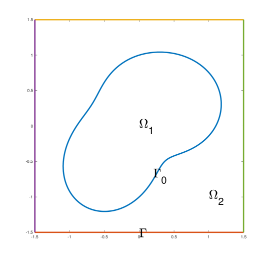
Figure 1: Illustration of the domain and the interface

Assume $\mathcal{A}$ to be discontinuous across $\Gamma_{0}$. We consider the interface problem below:

$$\left\{\begin{array}[]{rll}-{\rm div}\mathcal{A}^{2}\nabla u&=f&\mbox{in}\,\Omega_{1}\cup\Omega_{2},\\ u&=g&\mbox{on}\,\Gamma,\\ (\mathcal{A}^{2}\nabla u)|_{\Omega_{1}}\cdot\mathbf{n}_{1}+(\mathcal{A}^{2}\nabla u)|_{\Omega_{2}}\cdot\mathbf{n}_{2}&={\kappa_{2}}&\mbox{on}\,\Gamma_{0},\\ u|_{\Omega_{1}}-u|_{\Omega_{2}}&={\kappa_{1}}&\mbox{on}\,\Gamma_{0}.\end{array}\right.$$ (2.14)

The variational formulation is to find $u\in H^{1}(\Omega_{1})\times H^{1}(\Omega_{2}):=\{w\in L^{2}(\Omega):w|_{\Omega_{i}}\in H^{1}(\Omega_{i}),\ i=1,2\}$, such that

$$(\mathcal{A}^{2}\nabla u,\nabla v)_{\Omega_{1}\cup\Omega_{2}}=\langle f,v\rangle_{H^{-1}(\Omega)\times H^{1}_{0}(\Omega)}+\langle{\kappa_{2}},v\rangle_{\Gamma_{0}},\ \ \forall\,v\in H^{1}_{0}(\Omega),$$ (2.15)

and

$$u|_{\Gamma}=g,\ \ \mbox{and}\ \ \ u|_{\Omega_{1}}-u|_{\Omega_{2}}={\kappa_{1}}\ \ \text{on }\Gamma_{0}.$$ (2.16)

Here $\langle\cdot,\cdot\rangle_{\Gamma_{0}}$ is a duality between $H^{-1/2}(\Gamma_{0})$ and $H^{1/2}(\Gamma_{0})$, which evaluates as the $L^{2}$ inner product on $\Gamma_{0}$ for sufficiently smooth functions.

Theorem 2.5.

Let $u$ be the solution of (2.15)-(2.16), and $u^{*}$ be obtained by the four steps below:

1. Find a $\tilde{u}\in H^{1}(\Omega)$, such that

   $$(\mathcal{A}\nabla\tilde{u},\mathcal{A}\nabla v)_{\Omega}=\langle\tilde{f},v-\fint_{\Gamma}v\rangle+\langle{\kappa_{2}},v-\fint_{\Gamma}v\rangle_{\Gamma_{0}},\ \ \forall\,v\in H^{1}(\Omega).$$ (2.17)

2. Find a $\varphi\in H^{1}(\Omega)$, such that

   $$({\mathcal{A}^{-1}}{\rm curl}\varphi,{\mathcal{A}^{-1}}{\rm curl}\psi)_{\Omega_{1}\cup\Omega_{2}}=\langle\partial_{\mathbf{t}_{1}}{\kappa_{1}},\psi\rangle_{\Gamma_{0}}+\langle\partial_{\mathbf{t}}(g-\tilde{u}|_{\Gamma}),\psi\rangle_{\Gamma},\ \forall\,\psi\in H^{1}(\Omega).$$ (2.18)

3. Find a $u_{c}\in H^{1}(\Omega_{1})\times H^{1}(\Omega_{2})$, such that

   $$(\mathcal{A}\nabla u_{c},\mathcal{A}\nabla v)_{\Omega_{i}}=(\mathcal{A}\nabla\tilde{u}-\mathcal{A}^{-1}{\rm curl}\varphi,\mathcal{A}\nabla v)_{\Omega_{i}},\ \forall\,v\in H^{1}(\Omega_{i}),\,i=1,2.$$ (2.19)

4. Set $u^{*}|_{\Omega_{1}}=u_{c}|_{\Omega_{1}}-C_{1}$, $u^{*}|_{\Omega_{2}}=u_{c}|_{\Omega_{2}}-C_{2}$, with $C_{2}=\frac{1}{|\gamma|}\int_{\gamma}(u_{c}-g)$ for any $\gamma\subset\Gamma$ such that $|\gamma|\neq 0$, and $C_{1}=\frac{1}{|\gamma_{0}|}\int_{\gamma_{0}}(u_{c}|_{\Omega_{1}}-u^{*}|_{\Omega_{2}}-\kappa_{1})$ for any $\gamma_{0}\subset\Gamma_{0}$ such that $|\gamma_{0}|\neq 0$.

Then $u^{*}=u$.

Proof.

By the first item, $(\mathcal{A}^{2}\nabla(u-\tilde{u}),\nabla v)=0$ for $v\in H^{1}_{0}(\Omega)$, therefore, there exists $\varphi\in H^{1}(\Omega)$ such that $\mathcal{A}\nabla(u-\tilde{u})=\mathcal{A}^{-1}{\rm curl}\varphi$. It follows that ${\rm rot}\,\mathcal{A}^{-2}{\rm curl}\varphi=0$. Then

$$({\mathcal{A}^{-1}}{\rm curl}\varphi,{\mathcal{A}^{-1}}{\rm curl}\psi)_{\Omega_{i}} =\langle\mathcal{A}^{-2}{\rm curl}\varphi\cdot\mathbf{t}_{i},\psi\rangle_{\partial\Omega_{i}}$$

$$=\langle\nabla(u-\tilde{u})\cdot\mathbf{t}_{i},\psi\rangle_{\partial\Omega_{i}}=\langle\partial_{\mathbf{t}_{i}}(u|_{\partial\Omega_{i}}-\tilde{u}|_{\partial\Omega_{i}}),\psi\rangle_{\partial\Omega_{i}},$$

for any $\psi\in H^{1}(\Omega)$, and further

$$({\mathcal{A}^{-1}}{\rm curl}\varphi,{\mathcal{A}^{-1}}{\rm curl}\psi)_{\Omega_{1}\cup\Omega_{2}} =\sum_{i=1}^{2}\langle\partial_{\mathbf{t}_{i}}(u|_{\partial\Omega_{i}}-\tilde{u}|_{\partial\Omega_{i}}),\psi\rangle_{\partial\Omega_{i}}$$

$$=\langle\partial_{\mathbf{t}_{1}}{\kappa_{1}},\psi\rangle_{\Gamma_{0}}+\langle\partial_{\mathbf{t}}(g-\tilde{u}|_{\Gamma}),\psi\rangle_{\Gamma}.$$

The assertion follows immediately. ∎

Remark 2.6.

Again, it is helpful to understand the procedure by figuring out the respective strong forms related to equations (2.17)-(2.19).

1. By using integration by parts, we obtain the strong form of (2.17):

   $$\left\{\begin{array}[]{rll}-\nabla\cdot(\mathcal{A}^{2}\nabla\tilde{u})&=f,&\mbox{in}\,\Omega_{1}\cup\Omega_{2},\\ \mathbf{n}_{1}\cdot(\mathcal{A}^{2}\nabla\tilde{u})|_{\Omega_{1}}+\mathbf{n}_{2}\cdot(\mathcal{A}^{2}\nabla\tilde{u})|_{\Omega_{2}}&={\kappa_{2}},&\mbox{on}\,\Gamma_{0},\\ \mathbf{n}\cdot(\mathcal{A}^{2}\partial\tilde{u})&=-\frac{1}{|\Gamma|}\left(\langle f,1\rangle_{\Omega}+\langle k_{2},1\rangle_{\Gamma_{0}}\right),&\mbox{on}\,\Gamma.\end{array}\right.$$ (2.20)

2. The boundary value problem corresponding to (2.18) is:

   $$\left\{\begin{array}[]{rll}-{\rm rot}(\mathcal{A}^{-2}{\rm curl}\varphi)&=0&\mbox{in}\,\Omega_{1}\cup\Omega_{2},\\ \mathbf{t}_{1}\cdot(\mathcal{A}^{-2}{\rm curl}\varphi)|_{\Omega_{1}}+\mathbf{t}_{2}\cdot(\mathcal{A}^{-2}{\rm curl}\varphi)|_{\Omega_{2}}&=\partial_{\mathbf{t}_{1}}\kappa_{1},&\mbox{on}\,\Gamma_{0},\\ \mathbf{t}\cdot(\mathcal{A}^{-2}{\rm curl}\varphi)&=\partial_{\mathbf{t}}(g-\tilde{u}),&\mbox{on}\,\Gamma.\end{array}\right.$$ (2.21)

3. The boundary value problem corresponding to (2.19) is:

   $$\left\{\begin{array}[]{rll}-\nabla\cdot(\mathcal{A}^{2}\nabla u_{c})&=f,&\mbox{in}\,\Omega_{i},\\ \mathbf{n}_{i}\cdot(\mathcal{A}^{2}\nabla u_{c})-\mathbf{n}_{i}\cdot(\mathcal{A}^{2}\nabla\tilde{u})&=-\partial_{\mathbf{t}}\varphi,&\mbox{on}\,\partial\Omega_{i},\end{array}\right.$$ (2.22)

   for $i=1,2$.

From these strong forms, we see clearly that $\tilde{u}$ and $\phi$ are both continuous functions but with derivative jumps on interface $\Gamma_{0}$. This softens the jumps between $u_{c}|_{\Omega_{1}}$ and $u_{c}|_{\Omega_{2}}$ across $\Gamma_{0}$ on both function value and derivative jumps.

3 Natural deep Ritz methods

3.1 Natural deep Ritz method for Poisson equations with Dirichlet boundary conditions

Note that the three equations (2.2)-(2.3)-(2.4) in weak forms correspond to three elliptic equations with Neumann boundary conditions (2.5)-(2.6)-(2.7), which can be efficiently solved using Deep Ritz method without boundary penalty. Details are given in the following three steps. As usual, we use $\Phi_{NN}(d,1)$ for the set of neural network functions outputting a 1-dim vector with a d-dim input vector.

1. Find $u_{1}\in\Phi_{NN}(d,1)/\mathbb{R}$ by optimizing

   $$\mathcal{L}_{1}(u_{1}):=\Bigl{[}\sum_{\{x_{j},\omega_{j}\}\in\mathcal{D}}\frac{1}{2}|\nabla u_{1}(x_{j})|^{2}\omega_{j}-f(x_{j})(u_{1}(x_{j})-c_{1})\omega_{j}\Bigr{]}+c_{1}^{2},$$ (3.1)

   where $c_{1}=\frac{1}{|\mathcal{D}_{\Gamma}|}\sum_{\{x_{j},\omega_{j}\}\in\mathcal{D}_{\Gamma}}u_{1}(x_{j})\omega_{j}$. $\mathcal{D}$ and $\mathcal{D}_{\Gamma}$ are the set of quadrature points and weights for domain $\Omega$ and its boundary $\Gamma$. Hereby, the term $c_{1}^{2}$ is added in the objective function to make the solution unique.

2. Find $\varphi\in\Phi_{NN}(d,1)$ by optimizing

   $$\mathcal{L}_{2}(\varphi):= \sum_{\{x_{j},\omega_{j}\}\ \in\mathcal{D}}\frac{1}{2}[{\rm curl}\varphi(x_{j})]^{2}\omega_{j}+\sum_{\{x_{j},\omega_{j}\}\in\mathcal{D}_{\Gamma}}\bigl{[}g(x_{j})\partial_{\mathbf{\tau}}\varphi(x_{j})+\partial_{\mathbf{\tau}}u_{1}(x_{j})\varphi(x_{j})\bigr{]}\omega_{j}$$

   $$+\Bigl{[}\sum_{\{x_{j},\omega_{j}\}\in\mathcal{D}_{\Gamma}}\varphi(x_{j})\omega_{j}\Bigr{]}^{2}.$$ (3.2)

   Again, the last term is added to make the solution unique.

3. Find the solution $u_{c}\in\Phi_{NN}(d,1)$ by minimizing:

   $$\mathcal{L}_{3}(u_{c}):= \sum_{\{x_{j},\omega_{j}\}\in\mathcal{D}}\bigl{|}\nabla u_{c}(x_{j})-\nabla u_{1}(x_{j})+{\rm curl}\varphi(x_{j})\bigr{|}^{2}\omega_{j}$$

   $$+\Bigl{[}\sum_{\{x_{j},\omega_{j}\}\in\mathcal{D}_{\Gamma}}(u_{c}(x_{j})-g(x_{j}))\omega_{j}\Bigr{]}^{2}.$$ (3.3)

   The last term is a regularization term to make the integration of $u_{c}$ and $g$ on boundary $\partial\Omega$ equal to each other. Then, $u_{c}$ is a proper numerical approximation of $u$.

One may optimize the three equation (3.1)-(3.3) one by one, or optimize $\mathcal{L}_{1}+\mathcal{L}_{2}+\mathcal{L}_{3}$ all in one. To make the training procedure simpler, we take the latter approach in this paper.

The variable coefficient systems (2.17)-(2.18)-(2.19) can be solved similarly by the proposed natural deep Ritz method. We omit the details to save space.

3.2 Natural deep Ritz method for elliptic interface problems

For inteface problem defined in (2.17)-(2.18)-(2.19), it is more involved to design an efficient deep Ritz method. We will use similar approach as in the Poisson equations cases to solve (2.17)-(2.18), since both $u_{1}$ and $\varphi$ has no jump of function values on the interface $\Gamma_{0}$. We use two neural network functions to represent $u_{c}$, since it contains jumps on the interface $\Gamma_{0}$. We will solve (2.19) with two neural networks (or one neural network with two outputs $\Phi_{NN}(d,2)$), one for each subdomain $\Omega_{i},i=1,2$. The details are given below.

1. Find $u_{1}\in\Phi_{NN}(d,1)/\mathbb{R}$ by optimizing

   $$\mathcal{L}_{1}(u_{1}):= \Bigl{[}\sum_{\{x_{j},\omega_{j}\}\in\mathcal{D}}\frac{1}{2}|\nabla u_{1}(x_{j})|^{2}\mathcal{A}^{2}(x_{j})\omega_{j}-f(x_{j})(u_{1}(x_{j})-c_{1})\omega_{j}\Bigr{]}$$ (3.4)

   $$-\Bigl{[}\sum_{\{x_{j},\omega_{j}\}\in\mathcal{D}_{\Gamma_{0}}}\kappa_{2}(x_{j})(u_{1}(x_{j})-c_{1})\omega_{j}\Bigr{]}+c_{1}^{2},$$ (3.5)

   where $c_{1}=\frac{1}{|\mathcal{D}_{\Gamma}|}\sum_{\{x_{j},\omega_{j}\}\in\mathcal{D}_{\Gamma}}u_{1}(x_{j})\omega_{j}$. $\mathcal{D}$, $\mathcal{D}_{\Gamma}$ and $\mathcal{D}_{\Gamma_{0}}$ are the set of quadrature points and weights for domain $\Omega$, boundary $\Gamma$ and interface $\Gamma_{0}$.

2. Find $\varphi\in\Phi_{NN}(d,1)$ by optimizing

   $$\mathcal{L}_{2}(\varphi):= \sum_{\{x_{j},\omega_{j}\}\ \in\mathcal{D}}\frac{1}{2}[{\rm curl}\varphi(x_{j})]^{2}\mathcal{A}^{-2}(x_{j})\omega_{j}$$

   $$+\sum_{\{x_{j},\omega_{j}\}\in\mathcal{D}_{\Gamma}}\bigl{[}g(x_{j})\partial_{\mathbf{\tau}}\varphi(x_{j})+\partial_{\mathbf{\tau}}u_{1}(x_{j})\varphi(x_{j})\bigr{]}\omega_{j}$$

   $$+\Bigl{[}\sum_{\{x_{j},\omega_{j}\}\in\mathcal{D}_{\Gamma_{0}}}\kappa_{1}(x_{j})\partial_{\mathbf{\tau}}\varphi(x_{j})\omega_{j}\Bigr{]}+\Bigl{[}\sum_{\{x_{j},\omega_{j}\}\in\mathcal{D}_{\Gamma}}\varphi(x_{j})\omega_{j}\Bigr{]}^{2}.$$ (3.6)

   Note that the last term is added to make the solution unique.

3. Find the solution $(u^{c}_{1},u^{c}_{2})\in\Phi_{NN}(d,2)$ by minimizing:

   $$\mathcal{L}_{3}(u_{c}):= \sum_{i=1,2}\sum_{\{x_{j},\omega_{j}\}\in\mathcal{D}_{i}}\bigl{|}\mathcal{A}\nabla(u^{c}_{i}(x_{j})-u_{1}(x_{j}))+\mathcal{A}^{-1}{\rm curl}\varphi(x_{j})\bigr{|}^{2}\omega_{j}$$

   $$+\Bigl{[}\sum_{\{x_{j},\omega_{j}\}\in\mathcal{D}_{\Gamma}}(u^{c}_{2}(x_{j})-g(x_{j}))\omega_{j}\Bigr{]}^{2}$$

   $$+\Bigl{[}\sum_{\{x_{j},\omega_{j}\}\in\mathcal{D}_{\Gamma_{0}}}(u^{c}_{1}(x_{j})-u^{c}_{2}(x_{j})-\kappa_{1}(x_{j}))\omega_{j}\Bigr{]}^{2}.$$ (3.7)

   The last term is a regularization term to make the integration of $u_{c}$ and $g$ on boundary $\partial\Omega$ are equal to each other, such that $u_{c}$ is a proper numerical approximation of $u$.

Again, we will optimize $\mathcal{L}_{1}+\mathcal{L}_{2}+\mathcal{L}_{3}$ all in once.

4 Numerical experiments

We take $\Omega=[-1,1]^{2}$, and test following examples with given exact solutions.

• Example 1: A Poisson Dirichlet boundary value problem (1.1) with the exact solution

  $$u(x)=x_{1}^{2}+x_{2}^{2}+sin(x+y)$$ (4.1)

• Example 2: An elliptic equation with smooth variable coefficients and Dirichlet boundary condition (2.9). The variable coefficient matrix is taken as

  $$\mathcal{A}=\begin{pmatrix}1+x_{1}^{2},&0\\ 0,&1\end{pmatrix}.$$ (4.2)

  The exact solution is given as

  $$u(x)=\displaystyle e^{\cos\bigl{(}x_{1}+x_{2}^{2}\bigr{)}}.$$ (4.3)

• Example 3: An elliptic equation with non-smooth variable coefficients and Dirichlet boundary condition (2.9). The variable coefficient matrix is taken as

  $$\mathcal{A}=\begin{pmatrix}1+x_{1}^{2},&0\\ 0,&1+|x_{2}|\end{pmatrix}.$$ (4.4)

  The exact solution is taken as

  $$u(x)=\displaystyle e^{\cos\bigl{(}x_{1}+|x_{2}|^{3}\bigr{)}}.$$ (4.5)

• Example 4: An elliptic equation (2.9) with discontinuous coefficients. The coefficient matrix is taken as

  $$\mathcal{A}=\begin{pmatrix}1,&0\\ 0,&\frac{4}{3}-\frac{2}{3}\text{sgn}(x_{2})\end{pmatrix}.$$ (4.6)

  The exact solution is given as

  $$u(x)=e^{\cos(x_{1}+x_{2})}+\frac{1}{2}e^{\cos(x_{1}+|x_{2}|)}.$$ (4.7)

• Example 5: An interface problem (2.20)-(2.22). The domain $\Omega_{1}=[-0.5,0.5]^{2}$, $\Omega_{2}=\Omega\backslash\Omega_{1}$. The coefficient matrices are taken as

  $$\mathcal{A}|_{\Omega_{1}}=\begin{pmatrix}10,&0\\ 0,&10\end{pmatrix},\quad\mathcal{A}|_{\Omega_{2}}=\begin{pmatrix}1+x_{1}^{2},&0\\ 0,&1\end{pmatrix}.$$ (4.8)

  The exact solution is given as

  $$u(x)|_{\Omega_{1}}=5\displaystyle e^{-(x_{1}^{2}+x_{2}^{2})},\quad u(x)|_{\Omega_{2}}=4\displaystyle e^{\cos\bigl{(}x_{1}^{2}/2+x_{2}^{2}\bigr{)}-1}.$$ (4.9)

The implementation is conducted using PyTorch [29]. We employ ResNets with five ResBlock layers, where each ResBlock is a shallow network comprising 20, 35, and 35 hidden units for the proposed method, the standard deep Ritz method, and the PINN method, respectively, ensuring comparable parameter counts across these methods. We test activation functions ReCUr, Tanh, and ReQUr, with further details on ResNet structures and RePUr activations available in [9, 18, 41, 38].

For training data, we generate 10,000 inner and boundary points using composite Gaussian quadrature of order 5. An additional 10,000 points on a uniform grid serve as test data. The Adam optimizer is initially used to train the model for 100 epochs, with a batch size of 200 and an initial learning rate of 0.005. A learning rate scheduler, CosineAnnealingLR [23], is employed to adjust the learning rate. Following the Adam training phase, we further refine the model using the L-BFGS optimizer for 50 steps, with a history size of 100 and 60 inner iterations per step.

Results from both the proposed method and the standard deep Ritz method (using a boundary penalty constant $\beta=1000$) for these examples are presented in the following figures. We have several observations:

• By comparing 3 and 5, we observe that in the deep Ritz method, the boundary condition is quickly learned due to the large penalty constant $\beta=1000$. However, while this high penalty facilitates rapid boundary condition learning, it significantly slows the convergence of the solution within the domain, particularly for the Tanh network. We attribute this to the increased optimization complexity introduced by the large penalty. In contrast, the new penalty-free method learns both boundary values and the entire function inside the computational domain simultaneously, achieving a more accurate numerical solution with the same number of training points and training steps.

• The results for the two variable-coefficient cases, Examples 2 and 3, are comparable. The non-smoothness in the diffusion coefficients does not introduce significant additional difficulty, as the numerical error in the non-smooth coefficient case is only slightly higher than in the smooth coefficient case. Additionally, we observe that ReCUr DNNs outperform those using the other two activation functions, with RePUr DNNs demonstrating faster feature learning than Tanh networks, particularly during the Adam training phase.

• During training with Adam, ReQUr networks typically perform well; however, their performance occasionally degrades during the LBFGS training steps, particularly when compared to ReCUr, RePU4r, and Tanh networks. This may be due to the LBFGS method’s reliance on high-order information, and the higher-order derivatives of ReQUr networks are less smooth than those of the other networks.

  In the PINN results for Example 4 (Fig. 14), we observe that PINN performs poorly in this case compared to the proposed natural deep Ritz method. This discrepancy arises because the exact solution is not a strong solution, while the PINN method depends on the strong form of the equation.

• For the interface problem in Example 5, the results in Fig. 15 and 16 indicate that the proposed natural deep Ritz method can efficiently solve the interface problem without requiring penalty parameter tuning for boundary conditions and interface jump conditions. The relative $L^{2}$ error is approximately $2.5\times 10^{-3}$, and the relative $L^{\infty}$ error for this test is around $5\times 10^{-3}$. However, the LBFGS optimizer is less efficient in this case than in previous examples. Developing more efficient training methods for interface problems warrants further investigation.

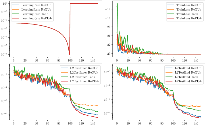
Figure 2: Training results : The learning rate (top-left), training loss (top-right) $L2$ Testing error on $\Omega$ (bottom-left) and boundary $\Gamma$ (bottom-right) for Example 1 using New method

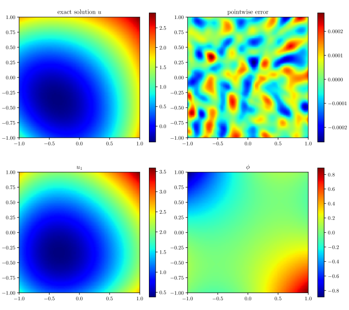
Figure 3: The exact solution and learned solution for Example 1 using New method

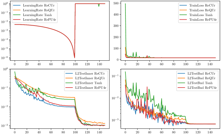
Figure 4: Training results : The learning rate (top-left), training loss (top-right) $L2$ Testing error on $\Omega$ (bottom-left) and boundary $\Gamma$ (bottom-right) for Example 1 using Deep Ritz method

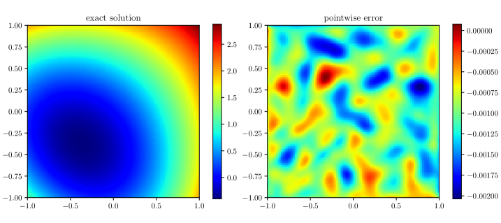
Figure 5: The exact solution and learned solution for for Example 1 using Deep Ritz method

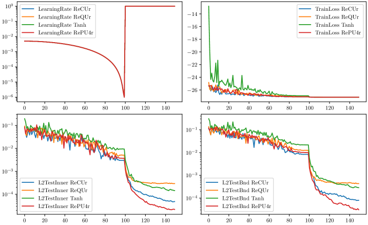
Figure 6: Training results : The learning rate (top-left), training loss (top-right) $L2$ Testing error on $\Omega$ (bottom-left) and boundary $\Gamma$ (bottom-right) for Example 2 using New method

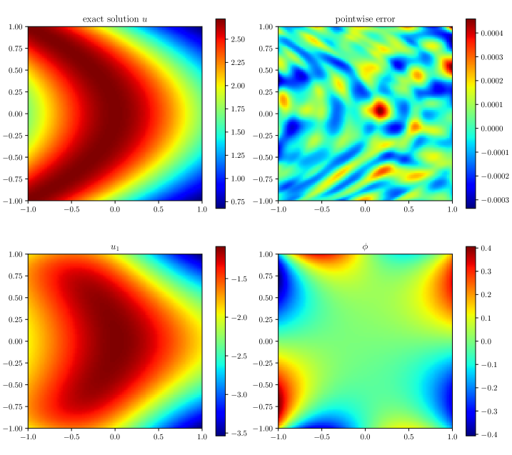
Figure 7: The exact solution and learned solution using RePUr neural networks for Example 2 using New method

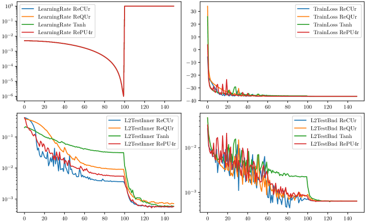
Figure 8: Training results : The learning rate (top-left), training loss (top-right) $L2$ Testing error on $\Omega$ (bottom-left) and boundary $\Gamma$ (bottom-right) for Example 2 using Deep Ritz method

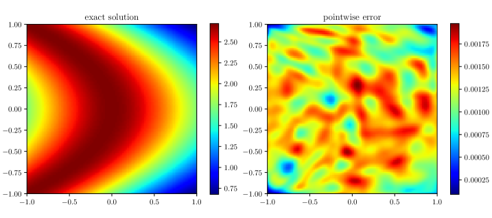
Figure 9: The exact solution and learned solution using RePUr neural networks for Example 2 using Deep Ritz method

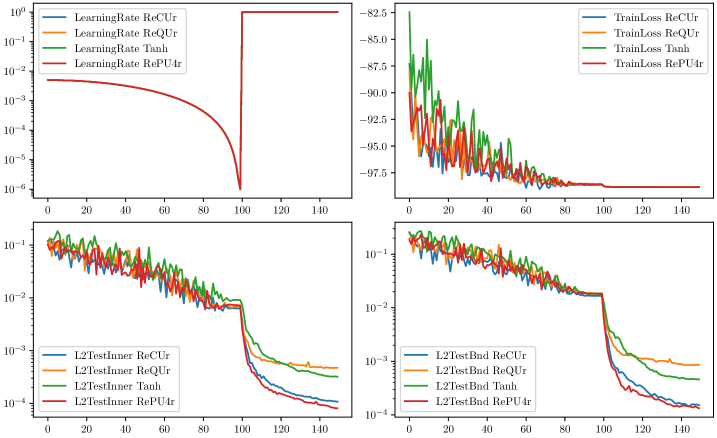
Figure 10: Training results : The learning rate (top-left), training loss (top-right) $L2$ Testing error on $\Omega$ (bottom-left) and boundary $\Gamma$ (bottom-right) for Example 3 using New method

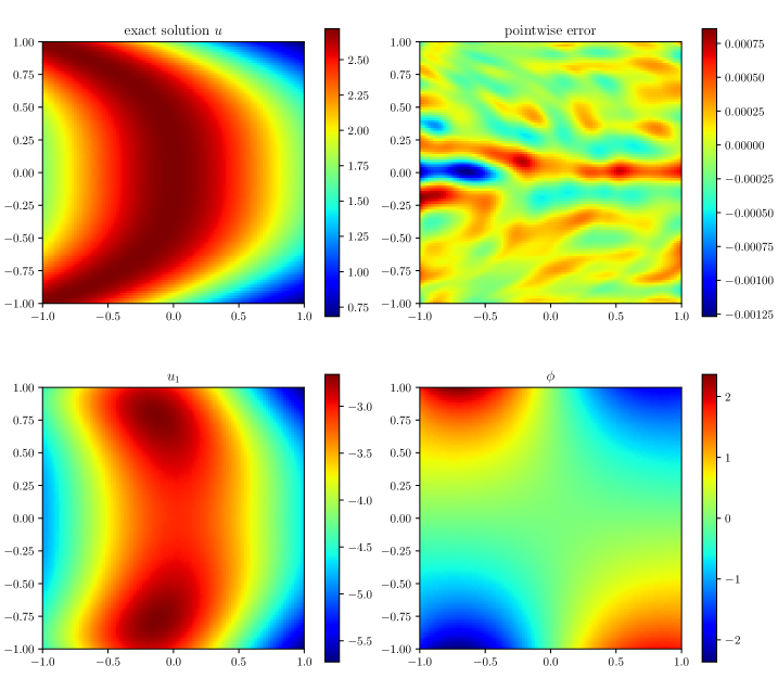
Figure 11: The exact solution and learned solution using RePUr neural networks for Example 3 using New method

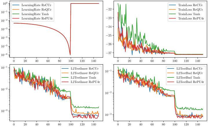
Figure 12: Training results : The learning rate (top-left), training loss (top-right) $L2$ Testing error on $\Omega$ (bottom-left) and boundary $\Gamma$ (bottom-right) for Example 4 using New method

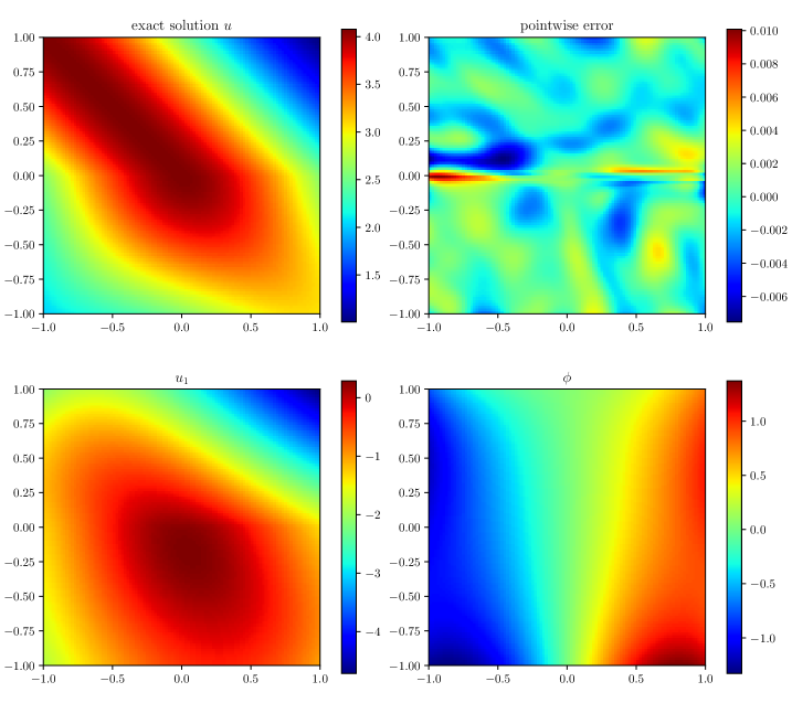
Figure 13: The exact solution and learned solution using RePUr neural networks for Example 4 using New method

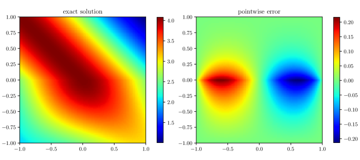
Figure 14: The exact solution and learned solution for Example 4 using PINN.

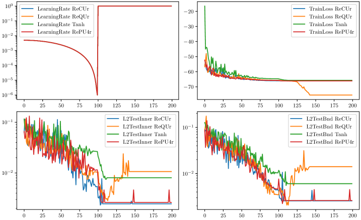
Figure 15: Training results : The learning rate (top-left), training loss (top-right) $L2$ Testing error on $\Omega$ (bottom-left) and boundary $\Gamma$ (bottom-right) for Example 5 using New method

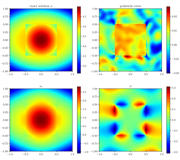
Figure 16: The exact solution and learned solution using RePUr neural networks for Example 4 using New method

5 Concluding remarks

In this paper, we develop a novel strategy for solving essential boundary value problems using neural networks by transforming the original problem into a series of pure natural boundary value problems, which can then be effectively solved using the deep Ritz method. Various model problems are employed to demonstrate the advantages of this approach. While this study focuses on two-dimensional elliptic problems with essential boundary conditions only, several potential extensions of the proposed method are possible:

1. Extension of the approach, readily, to other types of classical meshfree methods besides neural networks;

2. Extension to other boundary conditions, e.g. mixed type condition;

3. Extension to other self-adjoint problems provided relevant complex dualities, and the extension to non-self-adjoint problems is possible;

4. Extension, dedicatedly, to three-dimensional and higher dimensional problems.

We will present some of these extensions in future works.

References

References

- [1] Ivo Babuška. The finite element method with Lagrangian multipliers. Numerische Mathematik, 20(3):179–192, 1973.
- [2] Jens Berg and Kaj Nyström. A unified deep artificial neural network approach to partial differential equations in complex geometries. Neurocomputing, 317:28–41, 2018.
- [3] Xiaoli Chen, Beatrice W. Soh, Zi-En Ooi, Eleonore Vissol-Gaudin, Haijun Yu, Kostya S. Novoselov, Kedar Hippalgaonkar, and Qianxiao Li. Constructing custom thermodynamics using deep learning. Nat Comput Sci, 4:66–85, 2024.
- [4] Wolfgang Dahmen and Angela Kunoth. Appending boundary conditions by Lagrange multipliers: Analysis of the LBB condition. Numerische Mathematik, 88(1):9–42, 2001.
- [5] Weinan E and Bing Yu. The deep Ritz method: A deep learning-based numerical algorithm for solving variational problems. Communications in Mathematics and Statistics, 1(6):1–12, 2018.
- [6] Xavier Glorot, Antoine Bordes, and Yoshua Bengio. Deep sparse rectifier neural networks. In Proceedings of the 14 Th International Con- Ference on Artificial Intelligence and Statistics, volume 15, pages 315–323, Fort Lauderdal, 2011. JMLR.
- [7] Ian Goodfellow, Jean Pouget-Abadie, Mehdi Mirza, Bing Xu, David Warde-Farley, Sherjil Ozair, Aaron Courville, and Yoshua Bengio. Generative adversarial nets. In Z. Ghahramani, M. Welling, C. Cortes, N. Lawrence, and K.Q. Weinberger, editors, Advances in Neural Information Processing Systems, volume 27. Curran Associates, Inc., 2014.
- [8] Juncai He, Lin Li, Jinchao Xu, and Chunyue Zheng. ReLU deep neural networks and linear finite elements. Journal of Computational Mathematics, 38(3):502–527, 2020.
- [9] Kaiming He, Xiangyu Zhang, Shaoqing Ren, and Jian Sun. Deep residual learning for image recognition. In 2016 IEEE Conf. Comput. Vis. Pattern Recognit. CVPR, pages 770–778, 2016.
- [10] Geoffrey E. Hinton, Simon Osindero, and Yee-Whye Teh. A fast learning algorithm for deep belief nets. Neural Computation, 18(7):1527–1554, 2006. 8885 citations (Crossref) [2022-02-15].
- [11] J. J. Hopfield. Neural networks and physical systems with emergent collective computational abilities. PNAS, 79(8):2554–2558, April 1982. 12600 citations (Crossref) [2024-03-18] tex.ids: hopfieldNeuralNetworksPhysical1982.
- [12] Jianguo Huang, Haoqin Wang, and Tao Zhou. An augmented lagrangian deep learning method for variational problems with essential boundary conditions. Communications in Computational Physics, 31(3):966–986, 2022.
- [13] Yuehaw Khoo, Jianfeng Lu, and Lexing Ying. Solving parametric PDE problems with artificial neural networks. European Journal of Applied Mathematics, 32(3):421–435, 2021.
- [14] Diederik P. Kingma and Jimmy Ba. Adam: A Method for Stochastic Optimization. In arXiv:1412.6980 [Cs], San Diego, CA, USA, 2015.
- [15] Isaac E Lagaris, Aristidis Likas, and Dimitrios I Fotiadis. Artificial neural networks for solving ordinary and partial differential equations. IEEE Transactions on Neural Networks, 9(5):987–1000, 1998.
- [16] Isaac E Lagaris, Aristidis C Likas, and Dimitris G Papageorgiou. Neural-network methods for boundary value problems with irregular boundaries. IEEE Transactions on Neural Networks, 11(5):1041–1049, 2000.
- [17] Hyuk Lee and In Seok Kang. Neural algorithm for solving differential equations. Journal of Computational Physics, 91(1):110–131, 1990.
- [18] Bo Li, Shanshan Tang, and Haijun Yu. Better approximations of high dimensional smooth functions by deep neural networks with rectified power units. Communications in Computational Physics, 27(2):379–411, 2020.
- [19] Bo Li, Shanshan Tang, and Haijun Yu. PowerNet: Efficient representations of polynomials and smooth functions by deep neural networks with rectified power units. J. Math. Study, 53(2):159–191, January 2020.
- [20] Xuejuan Li, Jie Ouyang, Qiang Li, and Jinlian Ren. Integration wavelet neural network for steady convection dominated diffusion problem. In 2010 Third International Conference on Information and Computing, volume 2, pages 109–112. IEEE, 2010.
- [21] Yulei Liao and Pingbing Ming. Deep Nitsche method: Deep Ritz method with essential boundary conditions. Communications in Computational Physics, 29(5):1365–1384, 2021.
- [22] Zichao Long, Yiping Lu, and Bin Dong. PDE-Net 2.0: Learning PDEs from data with a numeric-symbolic hybrid deep network. Journal of Computational Physics, 399:108925, 2019.
- [23] Ilya Loshchilov and Frank Hutter. SGDR: Stochastic gradient descent with warm restarts. In ICLR 2017, 2017.
- [24] Liyao Lyu, Zhen Zhang, Minxin Chen, and Jingrun Chen. MIM: A deep mixed residual method for solving high-order partial differential equations. J. Comput. Phys., 452:110930, 2022.
- [25] Nam Mai-Duy and Thanh Tran-Cong. Numerical solution of differential equations using multiquadric radial basis function networks. Neural networks, 14(2):185–199, 2001.
- [26] Kevin Stanley McFall. Automated design parameter selection for neural networks solving coupled partial differential equations with discontinuities. Journal of the Franklin Institute, 350(2):300–317, 2013.
- [27] Kevin Stanley McFall and James Robert Mahan. Artificial neural network method for solution of boundary value problems with exact satisfaction of arbitrary boundary conditions. IEEE Transactions on Neural Networks, 20(8):1221–1233, 2009.
- [28] Joachim Nitsche. Über ein variationsprinzip zur lösung von Dirichlet-problemen bei verwendung von Teilräumen, die keinen randbedingungen unterworfen sind. In Abhandlungen aus dem mathematischen Seminar der Universität Hamburg, volume 36(1), pages 9–15. Springer, 1971.
- [29] Adam Paszke, Sam Gross, Francisco Massa, and et al. Pytorch: An imperative style, high-performance deep learning library. In Adv. Neural Inf. Process. Syst. 32, pages 8026–8037, 2019.
- [30] Philipp. Petersen and Felix. Voigtlaender. Optimal approximation of piecewise smooth functions using deep relu neural networks. Neural networks : the official journal of the International Neural Network Society, 108:296–330, 2018.
- [31] Maziar Raissi, Paris Perdikaris, and George E Karniadakis. Physics-informed neural networks: A deep learning framework for solving forward and inverse problems involving nonlinear partial differential equations. Journal of Computational physics, 378:686–707, 2019.
- [32] Maziar Raissi, Alireza Yazdani, and George Em Karniadakis. Hidden fluid mechanics: Learning velocity and pressure fields from flow visualizations. Science, 367(6481):1026–1030, 2020.
- [33] Zuowei Shen, Haizhao Yang, and Shijun Zhang. Deep network approximation characterized by number of neurons. Communications in Computational Physics, 28(5):1768–1811, 2020.
- [34] Hailong Sheng and Chao Yang. Pfnn: A penalty-free neural network method for solving a class of second-order boundary-value problems on complex geometries. Journal of Computational Physics, 428:110085, 2021.
- [35] Justin Sirignano and Konstantinos Spiliopoulos. DGM: A deep learning algorithm for solving partial differential equations. Journal of Computational Physics, 375:1339–1364, 2018.
- [36] Rolf Stenberg. On some techniques for approximating boundary conditions in the finite element method. Journal of Computational and Applied Mathematics, 63(1-3):139–148, 1995.
- [37] Shanshan Tang, Bo Li, and Haijun Yu. ChebNet: Efficient and stable constructions of deep neural networks with rectified power units via chebyshev approximation. Commun. Math. Stat., October 2024.
- [38] Xinyuan Tian, Shiqin Liu, and Haijun Yu. Deep neural networks with rectified power units: Efficient training and applications in partial differential equations. preprint, 2024.
- [39] B Ph van Milligen, V Tribaldos, and JA Jiménez. Neural network differential equation and plasma equilibrium solver. Physical Review Letters, 75(20):3594, 1995.
- [40] Jinchao Xu. Finite neuron method and convergence analysis. Communications in Computational Physics, 28(5):1707–1745, 2020.
- [41] Haijun Yu, Xinyuan Tian, Weinan E, and Qianxiao Li. OnsagerNet: Learning stable and interpretable dynamics using a generalized Onsager principle. Phys. Rev. Fluids, 6(11):114402, 2021.
- [42] Yaohua Zang, Gang Bao, Xiaojing Ye, and Haomin Zhou. Weak adversarial networks for high-dimensional partial differential equations. Journal of Computational Physics, 411:109409, 2020.
- [43] Dongkun Zhang, Ling Guo, and George Em Karniadakis. Learning in modal space: Solving time-dependent stochastic PDEs using physics-informed neural networks. SIAM Journal on Scientific Computing, 42(2):A639–A665, 2020.