Deep learning robotics using self-supervised spatial differentiation drive autonomous contact-based semiconductor characterization

Abstract

Integrating autonomous contact-based robotic characterization into self-driving laboratories can enhance measurement quality, reliability, and throughput. While deep learning models support robust autonomy, current methods lack pixel-precision positioning and require extensive labeled data. To overcome these challenges, we propose a self-supervised convolutional neural network with a spatially differentiable loss function, incorporating shape priors to refine predictions of optimal robot contact poses for semiconductor characterization. This network improves valid pose generation by 20.0%, relative to existing models. We demonstrate our network’s performance by driving a 4-degree-of-freedom robot to characterize photoconductivity at 3,025 predicted poses across a gradient of perovskite compositions, achieving throughputs over 125 measurements per hour. Spatially mapping photoconductivity onto each drop-casted film reveals regions of inhomogeneity. With this self-supervised deep learning-driven robotic system, we enable high-precision and reliable automation of contact-based characterization techniques at high throughputs, thereby allowing the measurement of previously inaccessible yet important semiconductor properties for self-driving laboratories.

Contact-based characterization techniques such as contact profilometry, four-point probes, and nanoindentation, among many others, are valuable tools in quantifying materials’ surface [1, 2, 3, 4, 5] and electrical properties [6, 7, 8, 9, 10]. By integrating deep learning and autonomous robotics into these methods, we can improve the reliability and quality of measurements [11, 12, 13], relieving researchers from the burden of constantly monitoring experiments to ensure optimal performance. However, integrating autonomy into these contact-based methods of characterization faces the challenges of reliably predicting high-precision contact positions [14, 15, 16], establishing high-throughput feedback control [17, 18], and collecting large labeled training datasets [19, 20]. Deep learning-controlled robotic measurement of material and molecular properties has been widely implemented across a range of optical characterization techniques [21, 22, 23, 24, 25, 26, 27], due to their non-contact nature, which simplifies mechanical complexity and increases data acquisition throughput compared to contact-based methods. For example, Su et al. [6] propose a robotic non-contact atomic force microscopy (nc-AFM) probe with positional control driven by the Faster Region-based convolutional neural network (Faster R-CNN) [28], which detects a general spatial bounding box around a target molecule for fast real-time positioning. However, the general bounding box is insufficient for orienting the pose of the robot to pixel-precise positions, and the model may require collecting additional labeled image data for fine-tuning [6]. Instead, the implementation of a self-supervised approach designed specifically for spatial positioning tasks has the potential to address these challenges, resulting in high-precision predictive robotic control with minimal data overhead.

Here, we propose the design of a self-supervised and spatially differentiable convolutional neural network (SDCNN) for optimal pose prediction of contact-based robotic characterization systems. We utilize this SDCNN to precisely and autonomously control a 4-degree-of-freedom (4DOF) robot with a four-point probe end effector to make optimal contact with each film and measure photoconductivity without going out of bounds, i.e., a valid robot contact pose. Each film is drop-casted using only 4 $\upmu$L of chemical precursor, which allows us to maximize the number of combinatorial perovskite compositions explored but produces small-area films that are difficult to characterize using contact-based approaches. Hence, implementing spatial differentiability into a CNN enables the computer vision-segmented films to be used as shape priors in the loss function for the refinement of predictions directly in image space, transforming an unsupervised learning problem into a self-supervised one. We demonstrate the general-use nature of the proposed SDCNN on two different characterization tasks of perovskite semiconductors: (1) surface profilometry and (2) photoconductivity. The robot pose prediction performance is then evaluated across three metrics: (1) positional accuracy, (2) rotational accuracy, and (3) valid pose generation. Our model’s performance across these metrics is compared to seven other CNN models with either conventional loss functions or robust loss functions from literature, such as Wing [29], Reverse Huber [30], and Barron [31], that are designed for spatial tasks. Our approach achieves a 20.0% improvement in the generation of valid poses, a 1.5% improvement in positional accuracy, and equivalent rotational accuracy compared to the robust loss functions from literature [29, 30, 31]. These performance improvements enable the practical viability of our approach for robot execution of contact-based measurements. We demonstrate this by autonomously characterizing $3,025$ photoconductivity curves of drop-casted perovskite semiconductors within 24 hours using the SDCNN-controlled 4DOF robotic system, achieving high throughputs of over 125 measurements per hour. These experimentally characterized photoconductance values are then spatially mapped back onto each semiconductor film, providing an understanding of the formation of degradation. By achieving high-precision robotic spatial control for the characterization of semiconductors through self-supervised deep learning models, we unlock new potential for integrating autonomous robotics into the semiconductor development and discovery pipeline, ultimately improving the reliability and quality of measurements at high throughputs without human supervision.

Results

Workflow for autonomous robotic control using vision and CNNs

Figure 1: Autonomous robotic process workflow for contact-based characterization of semiconductors. a, Synthesized and annealed drop-casted semiconductor films are fed into the autonomous process, consisting of computer vision segmentation of the semiconductor films, prediction of optimal robot poses using a spatially differentiable CNN (SDCNN), distance-minimizing path planning, and then robotic control with subsequent measurement. b, Photoconductivity and surface profilometry (smoothed) use-cases of the robotic contact-based characterization process. c, Average positional and rotational accuracy across $3,500$ robot pose predictions with two standard deviation error bars for our proposed SDCNN method, compared against seven other models.

Through optimal pose prediction from computer vision inputs, we autonomously drive a 4DOF robot with a four-point probe end effector to characterize the photoconductive properties of semiconductors spatially. Figure 1a illustrates this autonomous control pipeline. Firstly, semiconductor films are drop-cast offline from the autonomous feedback loop using an OpenTrons volumetric pipetter [32]. Then, an on-board camera takes an image of the semiconductors, $\Phi_{\textrm{cam}}$, which is then rectified from the camera reference frame to the robot reference frame using a series of calibration matrices, $K$:

$$\Phi_{\mathrm{robot}}=K_{\mathrm{img\rightarrow robot}}\left(K_{\mathrm{cam\rightarrow img}}\Phi_{\mathrm{cam}}\right)\;,$$ (1)

where $K_{\mathrm{cam\rightarrow img}}$ rectifies $\Phi_{\textrm{cam}}$ from the camera to the image reference frame and then $K_{\mathrm{img\rightarrow robot}}$ rectifies $\Phi_{\textrm{img}}$ from the image to the robot reference frame. Once, in the same coordinate frame as the robot, the Fast Segment Anything Model (FastSAM) [33] is used to quickly find the edges of each drop-casted film, creating image segments, $I$. Next, optimal poses are predicted directly onto the image segments using the proposed SDCNN model, an 8-layer CNN with customized spatially differentiable loss function. The optimality of each pose is determined using $I$ as a prior in image space, which can be back-propagated into the network as a loss due to spatial differentiability. A stochastic Dijkstra’s planner [34] is used to find a travel route that minimizes the total distance to all predicted poses across all drop-casted films. Finally, the robot is controlled to each SDCNN-predicted pose to characterize the properties of the semiconductor at that location in space. The average positional and rotational accuracies of predicted poses by the SDCNN are shown to be higher than predictions coming from CNNs using existing loss functions (Fig. 1c), with improvements between 1.5% and 8.9%. Designing the SDCNN to predict poses with high positional accuracy and rotational uniqueness enables comprehensive spatial mapping of important measured semiconductor properties in the fewest number of poses.

The spatial mapping capabilities of this autonomous workflow can be generalized to function with different contact-based end effectors. Figure 1b highlights two characterization use cases: photoconductivity and surface profilometry. Photoconductivity is measured at each predicted pose by taking the difference between illuminated and dark current-voltage curves (Fig. 1b, left). The blue-shaded regions highlight the spread of the photoconductive properties across the area of a drop-casted methylammonium lead iodide (MAPbI₃) perovskite film for a set of $k=3$ poses, predicted by the SDCNN to maximize the unique spatial area measured. These results indicate that photoconductivity is generally uniform across the area of this particular film. Conversely, the thickness of the film varies largely by tens of micrometers, measured using surface profilometry at the same spatially predicted contact poses (Fig. 1b, right). Utilizing different end effectors with the same driving SDCNN model, shows the ability to precisely it becomes possible to spatially resolve important properties of semiconductor materials in an autonomous fashion.

Spatial differentiability for optimal robot pose prediction

Figure 2: Creating a spatially differentiable loss function for image-based pose prediction. a, Image segment pixels ($I_{X},I_{Y}$) are passed through a Gaussian filter to maintain the differentiability of the edges. Predicted pose pixels, $(\mathrm{Pose}_{X},\mathrm{Pose}_{Y})$, from the SDCNN are superimposed onto the differentiable segment pixels, ($I^{\prime}_{X},I^{\prime}_{Y}$), using another Gaussian filter and sigmoid function, $S(\cdot)$, to perform direct computation and back-propagation in image space. b, SDCNN architecture and differential predicted poses, $(\mathrm{Pose}^{\prime}_{X},\mathrm{Pose}^{\prime}_{Y})$, composed onto the image segment pixels, ($I^{\prime}_{X},I^{\prime}_{Y}$). The SDCNN is trained to predict poses onto the regions of the films with high spatial reward (orange region).

Spatial differentiation enables our loss function to be differentiable across the pixel domain of an input, in turn, allowing for image-based computations to be back-propagated through the neurons of an SDCNN. Here, we use spatial differentiability to convert unsupervised learning into self-supervised learning by creating a pixel-based loss function that accepts shape priors as inputs to refine a prediction. We aim to have the SDCNN predict a set of $k$ valid robot poses that will maximize the number of pixels making unique contact with the spatial area of each film. The image segments, $I$, and predicted poses, $\{\mathrm{Pose}_{i}\}_{i=1}^{k}$, are the shape priors to the loss function. This method is valid for convex shapes in general and does not assume a perfect circle (Fig. S-5). These shapes are first passed through Gaussian filters to ensure they are smooth and differentiable before being passed to the loss function, generating, $I^{\prime}$ and $\{\mathrm{Pose}^{\prime}_{i}\}_{i=1}^{k}$ (Fig. 2a). A predicted pose is a valid contact if all its pixels fall within the non-zero regions of the segment, otherwise, the pose is invalid. Pixels with zero values are considered the background. The SDCNN is trained to predict poses onto the pixel region of $I^{\prime}$ with high spatial reward towards its center (Fig. 2b), tuned by changing the standard deviation of the Gaussian filter, $\sigma$ (Fig. 2a). The spatially differentiable loss function consists of a tunable weighted sum of two optimization objectives: (1) maximization of the intersection of each pose with non-zero segment pixels and (2) maximization of the pose rotational variance to encourage pose uniqueness:

$$\begin{split}\mathrm{loss}\left(I^{\prime},\{\mathrm{Pose}^{\prime}_{i}\}_{i=1}^{k}\right)=&-\underbrace{\omega_{1}\sum_{i=1}^{k}\left(I^{\prime}_{XY}\circ\{\mathrm{Pose}^{\prime}_{XY_{i}}\}_{i=1}^{k}\right)}_{\text{Maximize intersection with segment}}-\underbrace{\omega_{2}\operatorname{Var}\left(\{\mathrm{Pose}^{\prime}_{\theta_{i}}\}_{i=1}^{k}\right)\vphantom{\sum_{i=1}^{k}}}_{\text{Maximize angular variance}}\\[4.30554pt] &\qquad\qquad\text{subject to}\quad\mathrm{Pose}^{\prime}_{i}\cap\mathrm{Pose}^{\prime}_{j}=\emptyset,\quad\forall\,i\neq j,\end{split}$$ (2)

where $\omega_{1}$ and $\omega_{2}$ are weights set to $\omega_{1}=\omega_{2}$ and $I^{\prime}_{XY}\circ\mathrm{Pose}^{\prime}_{XY}$ is the composition of the differentiable segment pixels onto the differentiable pose pixels. $\mathrm{Pose}^{\prime}_{XY_{i}}$ and $\mathrm{Pose}^{\prime}_{\theta_{i}}$ are the $XY$-pixel coordinates and the yaw-rotation angles, respectively, for $i\in\{1,..,k\}$ unique differentiable poses. The objectives are negated to form a loss and are subject to the constraint of reducing the number of overlapping pixels between any two unique predicted poses.

Figure 3: Comparison of performance across different CNN loss functions on the robot pose prediction task. a, Loss minimization procedure in image space using our spatially differentiable CNN (SDCNN). b, Predicted poses onto a subset of 9 experimentally synthesized semiconductor films for $k=3$ poses per film. Eight models are compared: ours (SDCNN), recent loss functions from literature designed for robust and spatial tasks (Reverse Huber [30], Wing [29], and Barron [31]), and conventional loss functions (mean squared error (MSE), mean absolute error (MAE), Huber, and Poisson negative log-likelihood). $N$-number of valid contact poses that fully intersect with the drop-casted film are shown in white, and invalid poses are shown in red. The photocurrent curve at each valid pose is measured experimentally using the robotic system. c, Left: poses output by the same stochastic process used for generating the ground truth poses to train the conventional and robust models. Middle: success rate of generating $k=3$ valid poses for each film in the full set of 35 experimentally synthesized semiconductors across 100 unique trials. Right: computational performance of CNN inference time on the pose prediction task for the full set of films across 100 unique trials, run on an NVIDIA Tesla V100 GPU.

Figure 3a illustrates this loss minimization procedure in image space. Before training, the network has a high loss since it has not learned how to use the shape priors, resulting in placing poses randomly. After training, the network learns to place poses in high-reward regions of shape priors. Figure 3b compares the performance on the valid pose prediction task of our SDCNN against 7 other CNN models that use existing loss functions. Corresponding photoconductivity curves are experimentally measured on the perovskite film using the 4DOF robotic system for each valid predicted pose. The CNN models for comparison use either recent loss functions from literature designed for robust and spatial tasks [29, 30, 31] or conventional loss functions. Aside from the loss function, all models have equivalent network architectures and training parameters. However, since the models using existing loss functions are supervised, a labeled set of poses for each input segment is generated using a stochastic process (Fig. 3c, left). The models using existing loss functions tend to cluster predicted poses tightly together, often resulting in close or partial overlaps. In contrast, our approach encourages predictions to be more spread apart, effectively utilizing the full segment prior, while still being within the segment boundaries. Furthermore, in addition to tight clustering, as shown in Fig. 3b, the existing models also have lower positional accuracy (Fig. 1c), resulting in fewer valid poses being successfully generated for this subset of 9 perovskite films, compared to our spatially differentiable model.

In Fig. 3c (middle), we expand this analysis from 9 films to 35 films and perform 100 replicate trials of valid pose generation. Across these 100 trials, we demonstrate that our SDCNN model achieves improvements of 20.0% and 16.2% in the median success rate of generating valid poses over robust loss functions and conventional loss functions, respectively. Given these performance improvements, the inference time of our loss function is negligible compared to the hardware response time, increasing by only 2.4 ns, relative to the slowest tested loss function in our evaluation, Reverse Huber (Fig. 3c, right). Hence, utilizing spatial differentiability in a neural network for pose prediction tasks improves the reliability of autonomous robotics by successfully generating valid predictions without sacrificing compute speed, while also reducing the data labeling burden through self-supervision.

Autonomous characterization of perovskite photoconductivity

Figure 4: Photoconductivity of perovskite semiconductors characterized by an autonomous robotic platform controlled by a spatially differentiable CNN. a, Photoconductance, $G_{\mathrm{ph}}$, measured at $3,025$ unique poses, predicted by the spatially differentiable CNN (SDCNN), across a gradient of drop-casted methylammonium lead bromide (MAPbBr₃) to methylammonium lead iodide (MAPbI₃) mixed-halide perovskite semiconductor films, MAPb(Br_1-xI_x)₃. b, All measured photocurrent, $I_{\mathrm{ph}}$, curves with colormap corresponding to $G_{\mathrm{ph}}$ (slope of $I_{\mathrm{ph}}$). Measured $I_{\mathrm{ph}}$ curves for the following perovskite film compositions: c, MAPb(Br_0.94I_0.06)₃, d, MAPb(Br_0.47I_0.53)₃, and e, MAPb(Br_0.03I_0.97)₃. f, Top: images of synthesized MAPb(Br_1-xI_x)₃ films. Bottom: spatially mapped $G_{\mathrm{ph}}$ with Gaussian interpolation, collected using the autonomous robotic system. g, Perovskite films with non-uniform spatially-resolved $G_{\mathrm{ph}}$.

Semiconductor self-driving laboratories are capable of rapidly synthesizing materials that must be quickly screened for photoactivity to identify compositions yielding functional semiconductors for applications like solar cells [35, 36, 37] and light-emitting diodes (LEDs) [38, 39]. This need motivates the development of our coupled SDCNN and 4DOF contact-based robotic probe to characterize semiconductor photoconductivity autonomously at high-throughputs using an illuminating four-point probe end effector. The measured semiconductors during the campaign are a gradient of drop-casted methylammonium lead bromide (MAPbBr₃) to methylammonium lead iodide (MAPbI₃) mixed-halide perovskite films, MAPb(Br_1-xI_x)₃. Throughout the duration of a 24-hour campaign, $3,025$ unique poses are predicted and measured by the SDCNN-controlled robotic system. Resulting in a characterization throughput of over 125 measurements per hour. At each SDCNN-predicted pose, the photocurrent, $I_{\mathrm{ph}}$, is measured as a function of voltage, $V$, by taking the difference between the illuminated and dark current-voltage curves. Then, photoconductance, $G_{\mathrm{ph}}$, can be characterized at each pose by computing the slope of each photocurrent-voltage curve:

$$G_{\mathrm{ph}}=\frac{I_{\mathrm{ph}}}{V}=\frac{I_{\mathrm{light}}-I_{\mathrm{dark}}}{V}\;.$$ (3)

Figure 4a shows all characterized values of $G_{\mathrm{ph}}$ across the gradient of drop-casted perovskites, measured at $3,025$ uniquely predicted contact poses by the SDCNN. The distribution of $G_{\mathrm{ph}}$ along the $y$-axis for each composition illustrates the spatial variance of photoconductance across the area of each film with median values shown as black diamonds. An increasing trend in $G_{\mathrm{ph}}$ is observed (dashed curve in Fig. 4a) as the composition shifts from MAPbBr₃ to MAPbI₃ under broad-band white light illumination. This is consistent with the decreasing bandgaps of the corresponding perovskite compositions from 2.3 to 1.6 eV [40], assuming similar thicknesses between samples.

Figure 4b displays the full experimentally measured photocurrent-voltage curves, measured at each predicted pose. The spatially characterized $I_{\mathrm{ph}}$ curves are highlighted for three perovskite films within the MAPb(Br_1-xI_x)₃ gradient: bromine-rich (Fig. 4c), mixed (Fig. 4d), and iodine-rich (Fig. 4e). Data collected across several spatially distinct contact points for a given film allows us to generate a spatial map of experimental $G_{\mathrm{ph}}$ values using a simple Gaussian interpolation (Fig. 4f, bottom). Detailed spatial mapping is critical for identifying defects or non-uniformities in material synthesis, which can significantly affect device performance. For example, based on the trend observed in Fig. 4a, we expect iodine-rich films to have higher $G_{\mathrm{ph}}$ values across the area of the film area with only some expected spatial variation. However, in certain instances (Fig. 4g), we observe regions of very low $G_{\mathrm{ph}}$ values, likely induced by early degradation or pinhole defects in the film. Hence, with highly resolved spatial data, which can now be collected in an autonomous and high-throughput fashion for key properties like photoconductance, the root causes of critical defects and non-uniformities can be better understood faster. In turn, the advancement of these autonomous spatial mapping capabilities supports the improvement of material and device quality within the semiconductor development pipeline.

Discussion

In this paper, we develop a spatially differentiable convolutional neural network (SDCNN) for reliable and accurate pose prediction of contact-based autonomous robotics. Spatial differentiability transforms unsupervised learning into self-supervised learning by passing computer vision-segmented shape priors into a loss function for the refinement of predictions directly within image space. The general nature of this approach is shown by controlling the pose of a 4DOF robot with pixel-wise precision to characterize several material properties of perovskite semiconductor films, including photoconductivity and surface profilometry. Compared to existing supervised methods [29, 30, 31], the proposed self-supervised SDCNN approach achieves significant performance improvements of up to 20.0% in the generation of valid robot contact poses for semiconductor property characterization. We showcase the performance and reliability of the proposed SDCNN-controlled robotic positioning system in a continuous 24-hour autonomous campaign by characterizing the photoconductivity of drop-casted mixed-halide MAPb(Br_1-xI_x)₃ perovskite semiconductor films at $3,025$ uniquely predicted contact poses, without human intervention. Enabling characterization at throughputs over 125 measurements per hour at different positions on film, thus generating a spatial map of experimentally derived material properties for every film in a high-throughput manner. Rapidly resolving spatial properties using this proposed autonomous method offers early insight into the formation of defects and degradation – features that adversely affect semiconductor quality and must be caught quickly to evaluate performance improvements in semiconductor fabrication lines [41, 42].

Although the proposed robotic system is designed for autonomous operation from input image to experimental measurement, its calibration and swapping of end effectors are currently limited to manual operation. This manual calibration process is often tedious and relies heavily on the skill and precision of the user, leading to varying results and potential inconsistencies in experimental outcomes [14]. To minimize this source of variance and enhance the reliability of the robotic system, automated calibration techniques could be employed in future developments. For instance, automated bed leveling and height mapping are widely used in current 3D printing systems to ensure reliable performance between prints or tool changes [43], utilizing sensors and control algorithms to detect and compensate for misalignments. Integrating similar methods, such as vision-based calibration systems [44], or machine learning for calibration tasks [45, 46], could further enhance precision and adaptability. These advancements would reduce dependency on user expertise, improve overall efficiency, and broaden the system’s applicability to quantify a wider range of significant material properties.

Moreover, the number of predicted robot poses by the SDCNN is currently limited to the output vector length specified during the training procedure. This means that changing the number of output poses requires retraining the entire model, which can be time-consuming. To address this limitation, future developments may involve incorporating conditional rules through mixtures of experts (MoE) [47] or transformer-based architectures [48, 49], which facilitate the generation of a conditional number of poses without requiring complete retraining. Incorporating dynamic neural networks [50] and conditional variational autoencoders [51] could further enhance the model’s ability to adaptively generate poses tailored to specific experimental requirements. Additionally, integrating techniques from active learning [52] could enable the model to selectively update itself with new data, reducing the need for extensive retraining. These future works aim to extend the accessibility of the developed system to users without domain expertise in robotics while broadening the versatility of the applied deep learning models.

With the developed self-supervised SDCNN model and corresponding 4DOF robotic system, we have demonstrated the integration of reliable autonomy with minimal data overhead into the contact-based characterization of semiconductor films, measuring at high throughputs of over 125 photoconductivity curves per hour. Our proposed method improves the automated quantification of critical surface and electrical material properties, addressing prior challenges in achieving reliable automation. This advancement between the coupling of deep learning and robotics for materials science takes a step toward improving and accelerating methods of spatially characterizing important semiconductor properties in an autonomous fashion, galvanizing the pipeline of self-driving materials research.

Methods

Perovskite material preparation

To prepare the MAPb(Br_1-xI_x)₃ gradient of perovskite semiconductors, we use OpenTrons mixing and drop-casting of 0.6M MAPbI₃ and 0.6M MAPbBr₃ precursor solutions. The MAPbI₃ precursor is prepared using a 4:1 ratio of dimethylformamide (DMF, $\geq$99.8%, Sigma-Aldrich) to dimethylsulfoxide (DMSO, $\geq$99.9%, Sigma-Aldrich) solvent and then dissolving a 1:1 ratio of methylammonium iodide (MAI, $>$99.9%, Greatcell Solar Materials) to lead iodide (PbI₂, 99.999% trace metal basis, Sigma-Aldrich) solutes into the solvent mixture using a vortex mixer. The MAPbBr₃ precursor is prepared using a 4:1 ratio of DMF:DMSO solvent and then dissolving a 1:1 ratio of MAI to lead bromide (PbBr₂, 99.999% trace metal basis, Sigma-Aldrich) solutes into the solvent mixture using a vortex mixer. Once the precursors are prepared, the OpenTrons pipettes gradated concentrations of each precursor into 35 smaller volume vials in serial. Then, mixing is induced for each of the 35 unique compositions by repeatedly aspirating and dispensing the fluid in the vials three times. Once mixed, 4 $\upmu$L of each solution is pipetted onto a glass slide that is pre-heated to 55^∘C to form an array of individual films on the glass slide. Before heating, the glass slide was washed with isopropyl alcohol (IPA, $\geq$ 99.5%, VWR). After drop-casting, the glass slide is transferred to a pre-heated hot plate and annealed at 150^∘C for 20 minutes.

Robot and end effector design

The 4DOF robot controlled by the SDCNN and used for the measurement of semiconductor properties is custom-built. The frame of the robot positioning system is built using 80/20 T-slotted aluminum extrusion rails. Three standard Nema 17 stepper motors and timing belts control the $XYZ$-positioning of the robot. A Bigtreetech Direct Octopus V1.1 control board with TMC2209 stepper motor drivers, each tuned for 0.75A of output current, are used to drive all Nema motors. The poses predicted by the SDCNN are converted to Marlin G-code, which is sent to the control board via Python serial communication to execute motion commands. The motor that controls the $Z$-positioning is affixed to a 3D-printed chassis and uses a ball screw to drive the $Z$-positioning of the end effector mount. The last motor that controls the $\theta$-positioning (yaw) is a Nema 17 pancake motor affixed to a 3D-printed end effector mount. To this mount, an Ossila four-point probe head is affixed. We design an anti-cantilever attachment for the neck of the probe using rigid stereolithography 3D printing to mitigate $Z$-positioning drift. Attached to the head of the probe is a 3D-printed mount for three high-powered LEDs used to angle light to measure the $I_{\mathrm{light}}$ of the film in contact. The LED mount is designed to maximize uniform spread of light while minimizing shading, in turn, improving the consistency of measured $I_{\mathrm{light}}$.

Spatially differentiable loss function construction

The spatially differentiable loss function accepts shapes as priors to refine predictions. However, to maintain differentiability within the spatial image domain, each shape’s edge must be smoothed. The shapes that get passed through the loss function are the computer vision segmentations of the semiconductor films, $I$, and the set of $k$ poses predicted by the SDCNN, $\{\mathrm{Pose}_{i}\}_{i=1}^{k}$. To maintain differentiability, the pixels of these shapes pass through a 2D Gaussian filter:

$$I^{\prime}_{XY}=\frac{1}{2\pi\sigma^{2}}\exp{\left(-\frac{I^{2}_{X}+I^{2}_{Y}}{2\sigma^{2}}\right)}\;,$$ (4)

where $\sigma$ is the standard deviation of the Gaussian and $I_{XY}$ are the non-differentiable $XY$-pixels of a segment. A composition is created by superimposing the predicted poses directly onto a differentiable segment:

$$I^{\prime}_{XY}\circ\mathrm{Pose}^{\prime}_{XY}=S\left(\exp{\left(-\frac{(I^{\prime}_{X}-\mathrm{Pose}_{X})^{2}+(I^{\prime}_{Y}-\mathrm{Pose}_{Y})^{2}}{2\sigma^{2}}\right)}\right)\;,$$ (5)

where $S(\cdot)$ is the sigmoid function, used as a soft threshold for placement of the poses onto the segment, $I^{\prime}_{XY}$ are the differentiable $XY$-pixels of a segment, and $\mathrm{Pose}_{XY}$ are the non-differentiable $XY$-pixels of a predicted pose. With this composition, differentiability within pixel space is ensured, and now all differentiable computations performed on the image can be backpropagated to the network weights during training. The loss function that we aim to minimize to train the network is expressed in Eq. 2.

Neural network architecture and training

We evaluate the performance of 8 different CNN models on the pose prediction task, each with the same 8-layer network architecture but with a different loss function: SDCNN (ours), robust spatial loss functions from literature (Wing [29], Reverse Huber [30], Barron [31]), and conventional loss functions (MSE, MAE, Poisson, Huber). Our 8-layer network consists of the following architecture: (1) $3\times 3$ convolution with batch normalization, (2) spatial attention mechanism, (3) $3\times 3$ convolution with batch normalization, (4) max pooling, (5) 50% dropout, (6) fully connected (FC) with $1,200$ neurons, (7) FC with $600$ neurons, (8) FC with $(k*3)$ neurons, where $3$ represents the $XY$ midpoint pixel and rotation angle, $\theta$, for $k$-number of poses, $\{(\mathrm{Pose}^{\prime}_{X_{i}},\mathrm{Pose}^{\prime}_{Y_{i}},\mathrm{Pose}^{\prime}_{\theta_{i}})\}_{i=1}^{k}$ (Fig 2b, top). Our spatial attention module, derived from the Convolutional Block Attention Module (CBAM) [53], is placed at the beginning of the network to emphasize or suppress large-scale geometric features of the input images to help place contact poses within the film boundaries. Our self-supervised SDCNN model is trained on 8,500 augmented images of experimentally synthesized perovskite drop-casted films with an 80/20 training-validation split. The spatially differentiable loss function directly transforms the input predicted poses to the optimization objective in Eq. 2 to minimize. For the remaining 7 CNNs, a set of labels is generated for the 8,500 training images using a stochastic process. Each label is generated by inputting $N=100$ randomly generated poses into Eq. 2 for every image. The pose with the lowest loss, $\mathrm{Pose}_{i^{*}}$, becomes the image label for training:

$$i^{*}=\arg\min_{i\in\{1,...,N\}}\;\mathrm{loss}\left(I,\mathrm{Pose}_{i}\right)\;.$$ (6)

Although this trial-and-error process is slow, it generates effective data labels for benchmark purposes using the same loss function construction as our SDCNN but without spatial differentiability. Thus, enabling meaningful comparisons between model results. Figure 3c (left) shows an example of the performance of this stochastic process for generating labeled image data.

Photoconductivity characterization

To characterize the photoconductive properties of each perovskite film, a Python-controlled Keithley 2425 source meter measures the resultant current from our SDCNN-driven robotic system with a four-point probe end effector. The current is measured at 40 unique voltage steps across a -40 V to 40 V voltage sweep for each contact pose to capture detailed current-response curves. This sweep is repeated twice for each contact, once in the dark and once under illumination to measure the photocurrent, $I_{\mathrm{ph}}$ (Eq. 3). Attached to the gold-tipped four-point probe end effector is a 3D-printed LED mount, which is controlled using Python commands sent to an Arduino microcontroller with solid-state relays. Illumination is provided by probe-mounted high-power white LEDs positioned 4 mm above the film surface. This setup ensured consistent and uniform lighting at an intensity of approximately 200 mW cm^-2 (2 suns). The 3D-printed LED mount for the probe head aligns the light beams of the LEDs with the goal of improving light distribution uniformity across the measurement area while avoiding shading effects. Additionally, the LEDs have a large viewing angle of 120^∘ to optimize the overlap of light beams, further improving the light distribution uniformity during each measurement.

Data Availability

All result files and model weights have been deposited in the OSF database under accession code: https://osf.io/sdy7k.

Code Availability

All code used to develop the SDCNN models is available publicly with complete working examples on GitHub: https://github.com/PV-Lab/SDCNN.

Author Contributions

A.E.S. conceptualized the work. A.E.S., B.D., K.J., and T.B. designed the methodology. A.E.S. wrote the software. A.E.S., B.D., and F.S. prepared the experimental materials. A.E.S. and B.D. conducted experiments. A.E.S. performed the analysis. A.E.S. wrote the manuscript. All authors reviewed and edited the manuscript. B.D., K.J., and T.B. provided guidance.

Competing Interests

The authors declare no competing interests.

Supplementary Information:
Deep learning robotics using self-supervised spatial differentiation drive autonomous contact-based semiconductor characterization

Alexander E. Siemenn^1∗, Basita Das¹, Kangyu Ji^1,2, Fang Sheng¹, Tonio Buonassisi¹

¹Department of Mechanical Engineering, Massachusetts Institute of Technology, Cambridge, MA 02139, USA

²Research Laboratory of Electronics, Massachusetts Institute of Technology, Cambridge, MA 02139, USA

^∗Corresponding author: asiemenn@mit.edu

Design

Robot control workflow

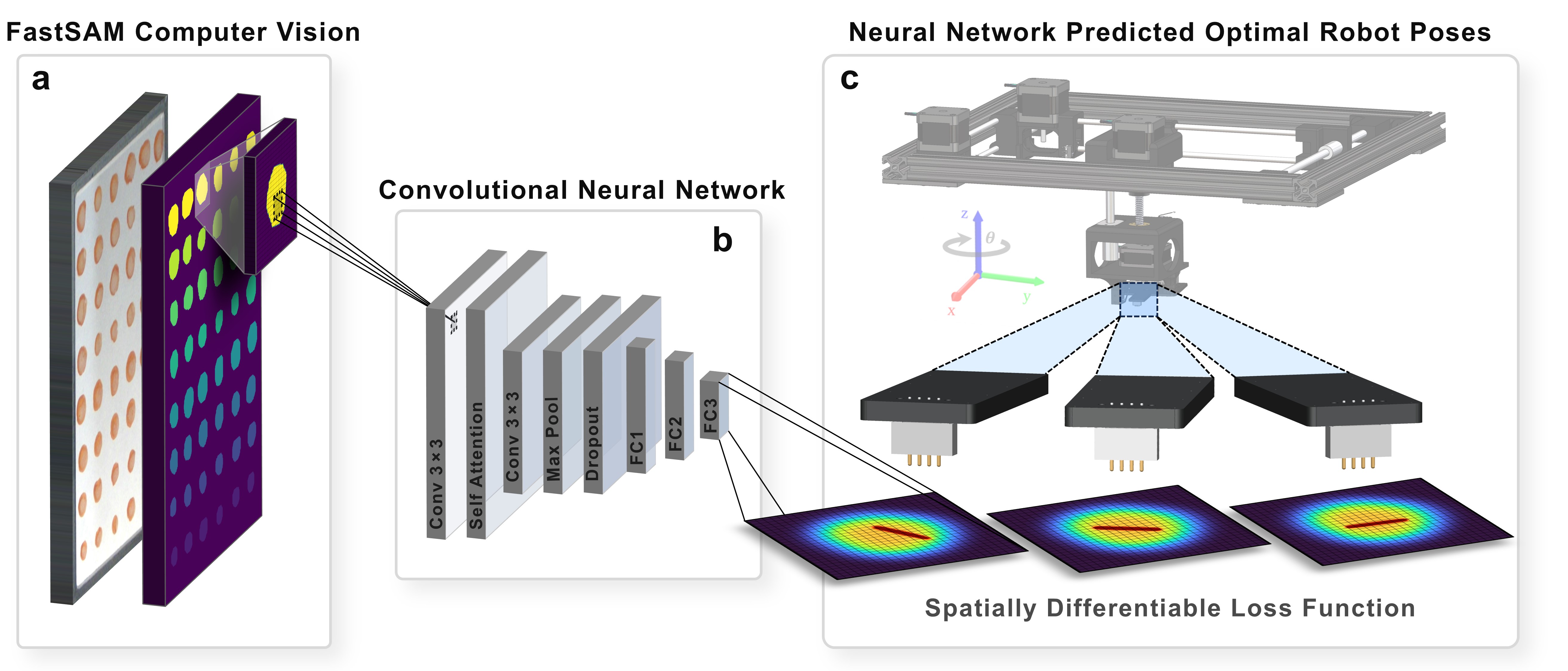
Figure S-1: Autonomous robotic workflow, zoomed in. a, The fast segment anything model (FastSAM) is used to quickly segment printed materials. These shapes are used as priors for the spatially differentiable convolutional neural network (SDCNN) predictions. b, SDCNN takes input shape priors, and outputs predicted poses. c, Control of robot motion based on the predicted poses.

In this paper, we autonomously control a 4-degree-of-freedom (4DOF) robot with an illuminating four-point probe end effector to measure the photoconductivity of semiconductors. In Fig. S-1, shape priors are used to output optimal poses for the robot to move to and measure each material. A geometric transfer function is used to control the motion of the end effector about the $\theta$-axis (yaw).

Robot calibration

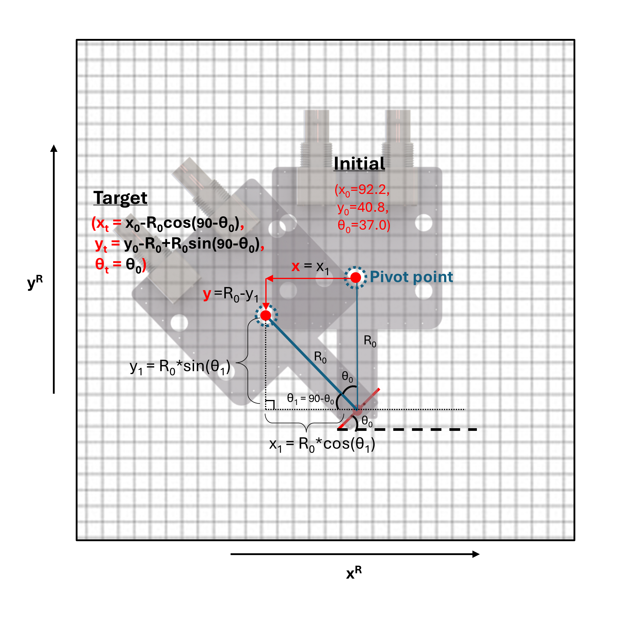
Figure S-2: Geometric transfer functions to achieve target poses of an end effector with a single pivot point.

Figure S-2 illustrates the mathematical procedure of achieving a target pose from an input set of coordinates. A geometric transformation is applied to ensure the contact point down the arm of the end effector meets the coordinates at the correct position in space:

$$x_{t} =x_{0}-R_{0}\mathrm{cos}(90-\theta_{0}),$$ (S-2)

$$y_{t} =y_{0}-R_{0}+R_{0}\mathrm{sin}(90-\theta_{0}),$$ (S-3)

$$\theta_{t} =\theta_{0},$$ (S-4)

where $x_{t}$, $y_{t}$, and $\theta_{t}$ are the target coordinates, given the initial coordinates $x_{0}$, $y_{0}$, and $\theta_{0}$ and $R_{0}$ is the measured length of the end effector arm from the pivot point to the desired contact point.

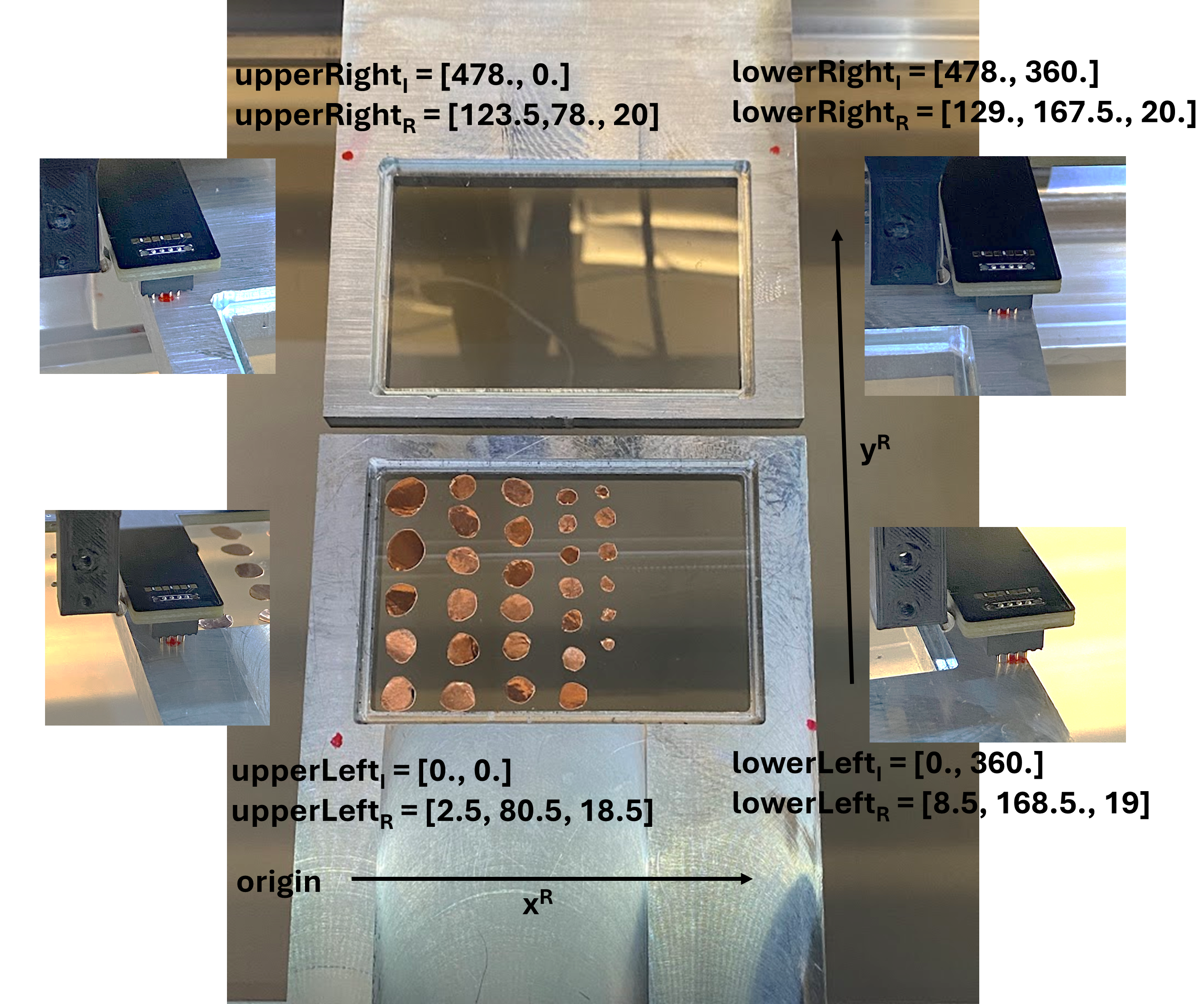
(a) Robot coordinate-pair calibration

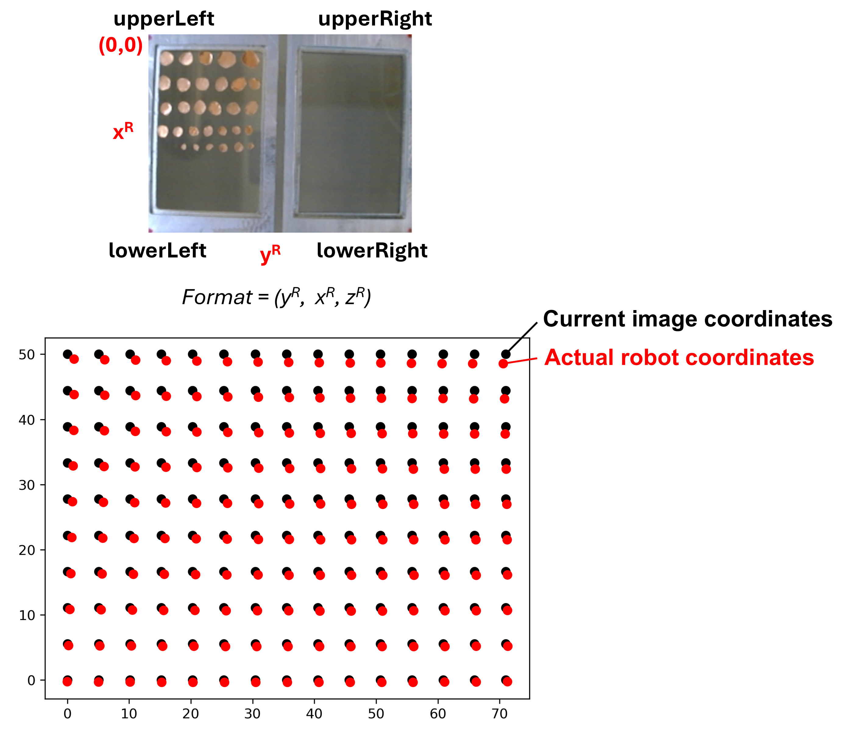
(b) Calibration Mesh

Figure S-3: Calibration procedure for the 4DOF robot. a, Manual calibration of image (I)-robot (R) coordinate pairs. b, Calibration mesh applied to the post-rectified coordinates.

To fully calibrate the robot positioning system, image-robot coordinate pairs are collected. These coordinate-pairs establish the robot’s location in space, given a set of image coordinates. Coordinate pairs are collected along the outer perimeter of the imaging field. Thus, the corners of the imaging field will align with the corners of the robot reference frame (S-3a). Due to lens effects and imperfect image rectification, there is still an image-robot coordinate mismatch if measured again after calibration. We measure 15 different image-robot coordinate pairs and generate a calibration mesh (Fig S-3b) to apply to the coordinates to ensure proper alignment of the robot within image space.

3D-printed LED mount

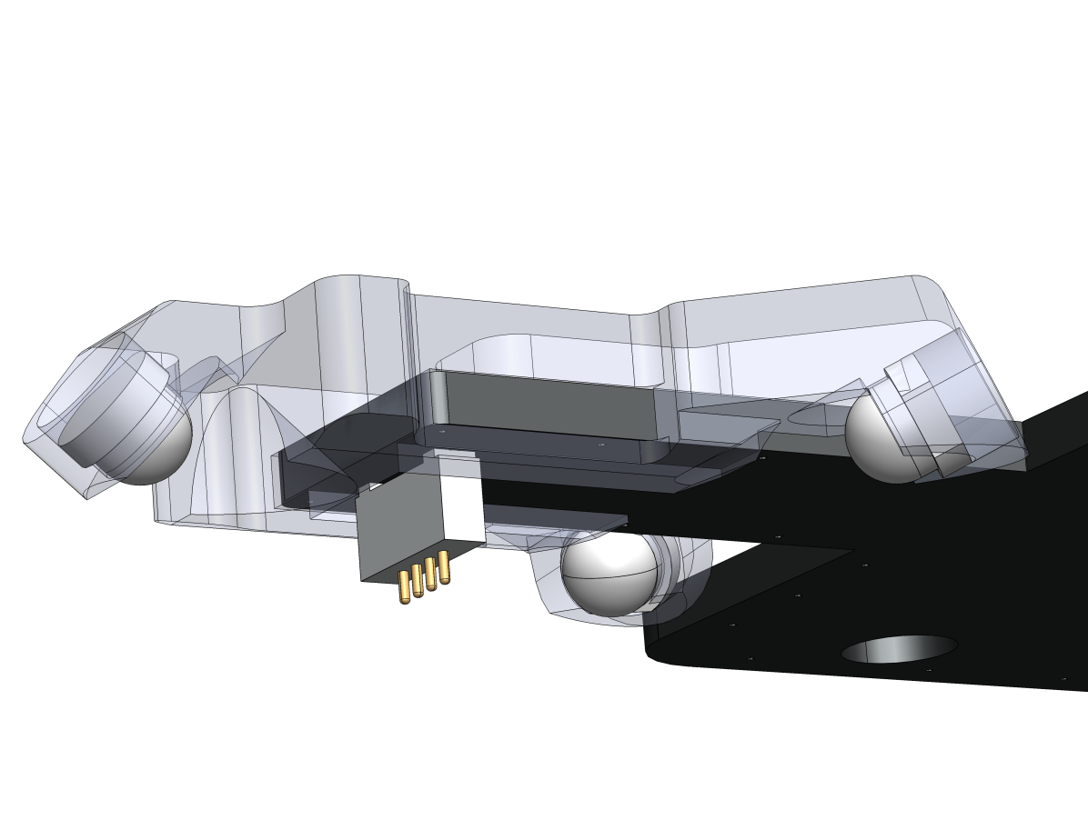
(a) Side view of mount

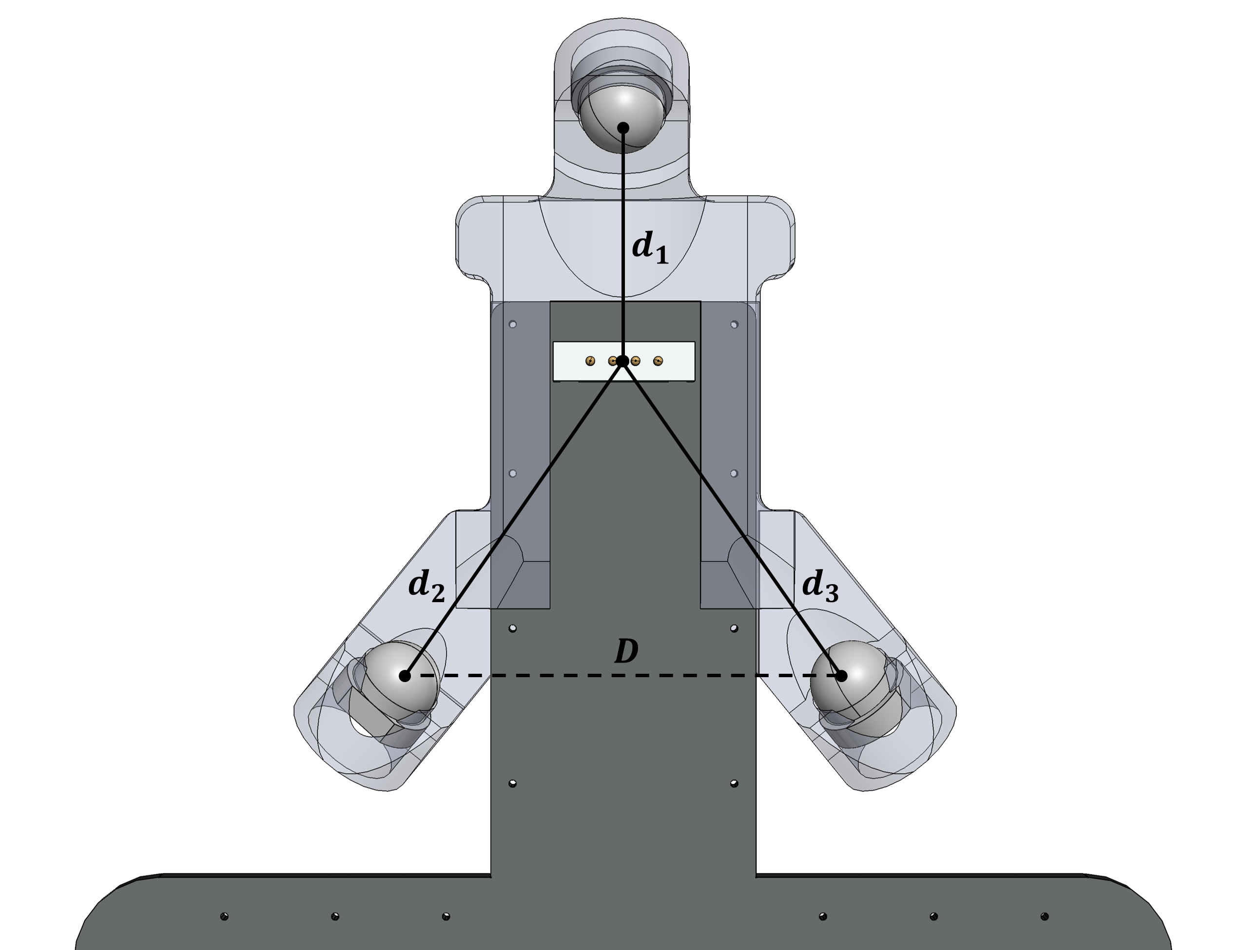
(b) Bottom view of mount

Figure S-4: Design of the 3D-printed LED mount to the four-point probe for photoconductivity measurement. a, Side view of the 3D printed mount. b, Bottom view of the 3D printed mount with calculated LED positions.

Fuse deposition modeling (FDM) 3D printing is used to create the LED mount for the four-point probe (Fig. S-4). Three LEDs are positioned as vertices to an isosceles triangle with the aim of maximizing illumination uniformity at the probe tips and minimizing shading. To minimize shading due to the probe tips, placing two LEDs, one in front and one behind the tips, would suffice. However, it is mechanically infeasible to place an LED behind the tips and still make contact with a material. Thus, we achieve this goal by positioning two LEDs to either side of the probe arm. To ensure uniform light distribution, these back LEDs are mounted farther away from the center point such that illumination intensity is not stronger, using the following relation:

$$d_{3}=d_{2}=\sqrt{(d_{1})^{2}-D^{2}}\;,$$ (S-5)

where $d_{3}$ and $d_{2}$ are the distances from the center point to either back LED, $D$ is the distance between the back LEDs, and $d_{1}$ is the distance from the center point to the front LED.

Experiments

Varying image inputs

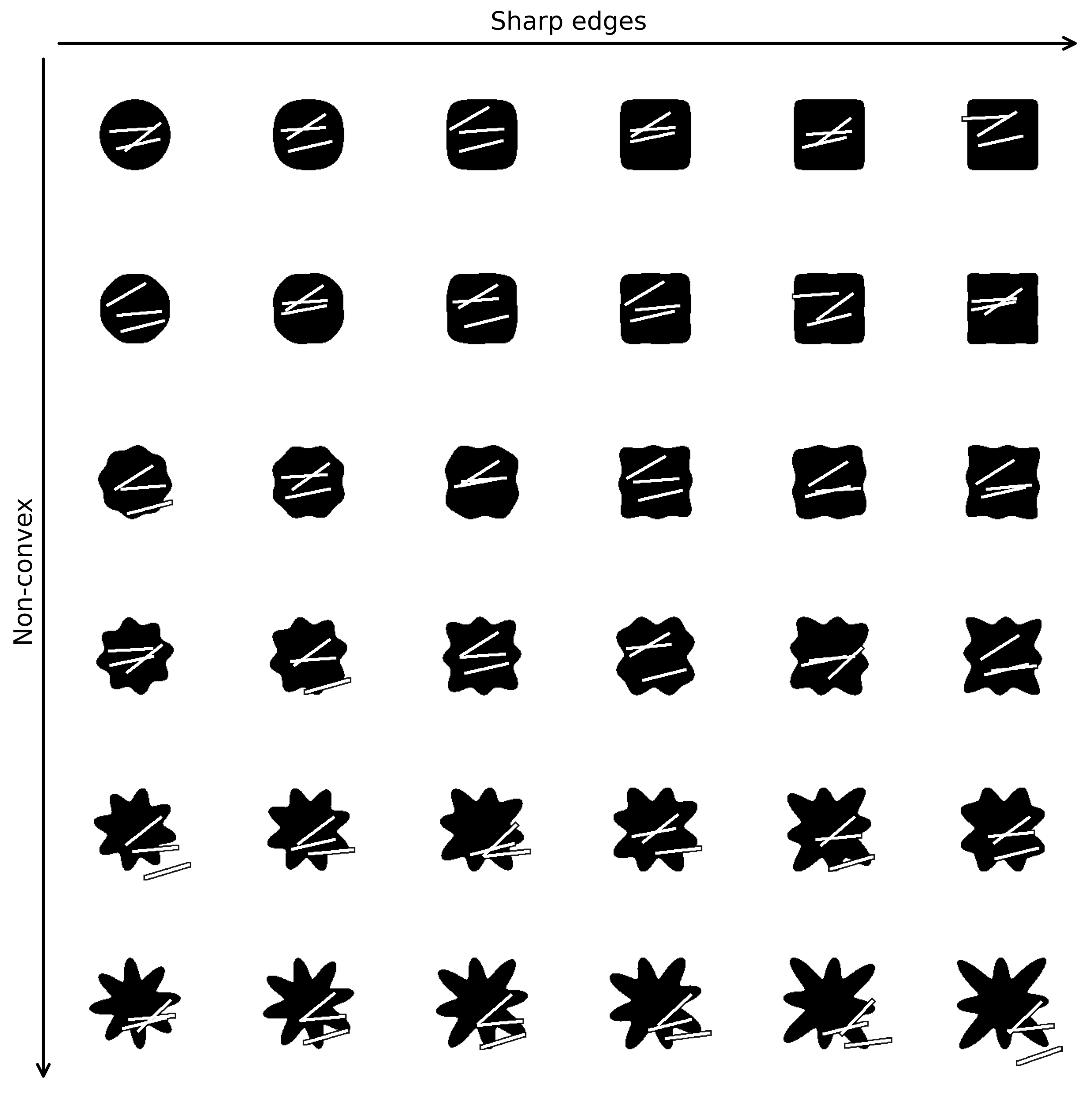
(a) Input segments with predictions

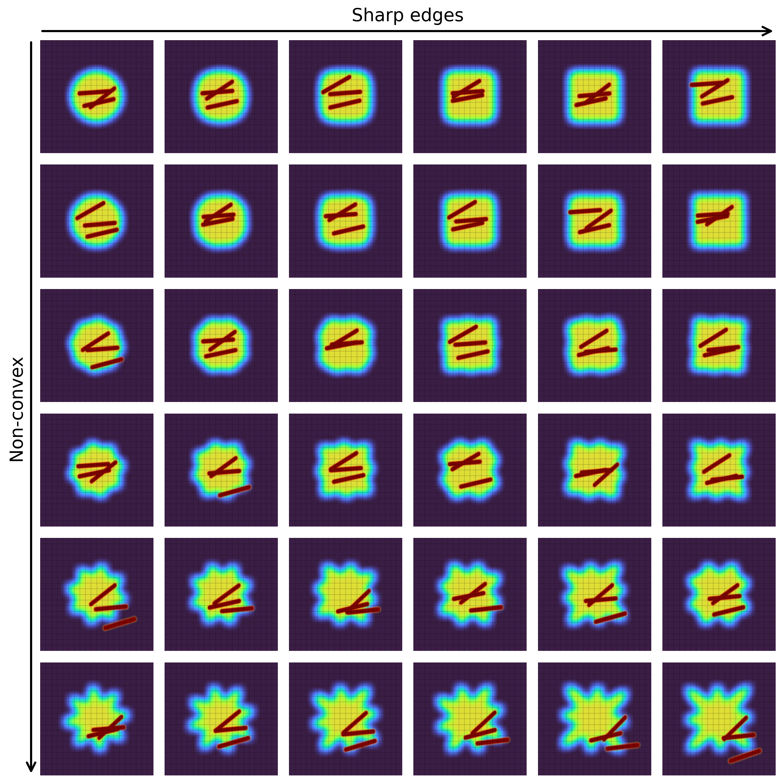
(b) Differentiable maps of input shapes

Figure S-5: SDCNN pose prediction on input shapes varying in edge sharpness and convexity. a, 6$\times$6 grid of various input shapes with predicted poses overlayed. b, 6$\times$6 grid showing the estimated differentiable maps for each input shape.

The shape of the input image segments to the SDCNN governs the placement of poses. With the presented version of the model, the weights are trained on rounded, convex shapes due to the nature of predicting poses for drop-casted semiconductor films. However, when we take this pre-trained model and apply it to input shapes with different formats, we get varying results. Figure S-5 illustrates how well this SDCNN performs for input shapes varying in edge sharpness and convexity. Model predictions are augmented with $k=3$ poses randomly selected from four predictions for each input to increase randomness and demonstrate robustness to the task. We see that, in general, this SDCNN performs best on convex and rounded input shapes (upper left), as these are most similar to its training set. Robustness to edge sharpness is demonstrated along the horizontal axis, but model performance breaks down as input shapes become more non-convex along the vertical axis. Here, predicted poses start to drift towards the edges, with many falling outside of the shape boundary. These results highlight the robustness of the model to certain features but also show the importance of training the SDCNN using shape priors that more closely align with the expected testing conditions.

Robot path following

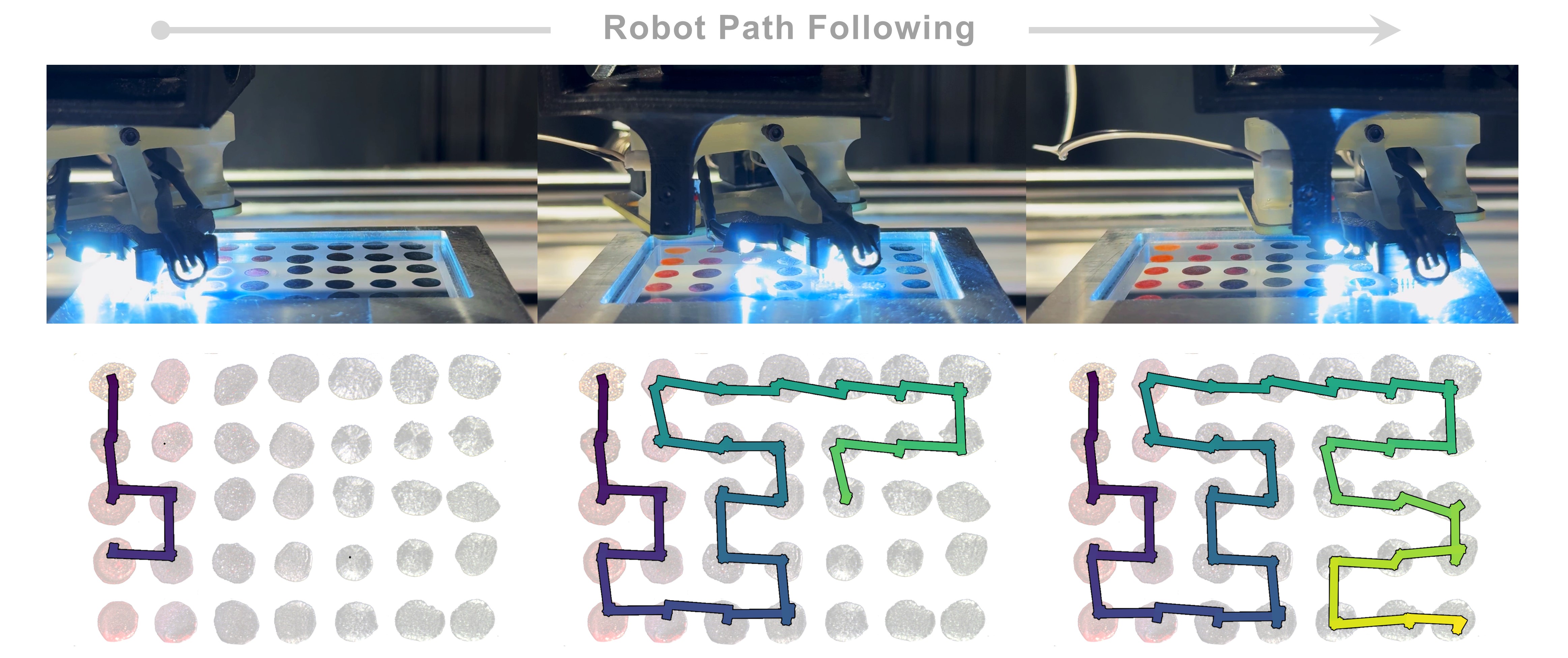
Figure S-6: 4DOF robot path following using a stochastic Dijkstra’s planner. Three snapshots in time are shown (top) of the robot following the generated path (bottom) to connect all predicted poses with the shortest travel distance.

After the SDCNN predicts the robot poses for measuring materials, a path must be generated for the robot to follow and execute each pose. A stochastic Dijkstra’s planner is used to generate an efficient route that connects all predicted poses with the shortest total travel time. Figure S-6 illustrates the non-trivial route that minimizes the travel distance between the grid of drop-casted films to measure.

Material characterization

Figure S-7: Varying illumination intensity on perovskite photocurrent. Current-voltage response increases as illumination intensity increases for a spun-coat FAPbI₃ (formamidinium lead iodide) perovskite thin film. Shaded regions indicate two standard deviations about the mean for each curve across 10 independent measurement trials.

We design the photoconductivity end effector of the 4DOF robot to have variable illumination control. Although we only need dark and illuminated conditions to characterize photoconductance, we calibrate the measurement on all quantized illuminations. Figure S-7 illustrates the current response dependence on illumination intensity for a spun-coat FAPbI₃ (formamidinium lead iodide) perovskite thin film. Six different LED illumination intensities are tested, as well as dark conditions. As the voltage supplied to the LEDs increases, the illumination intensity increases. As the illumination intensity increases, the photocurrent response of the FAPbI₃ film increases.

We characterize the crystal phase of the semiconductor films drop-casted by the OpenTrons overhead volumetric pipetter used in this study. Figure S-8 illustrates 14 X-ray diffraction (XRD) traces measured from 14 of the total 35 drop-casted methylammonium lead bromide (MAPbBr₃) to methylammonium lead iodide (MAPbI₃) mixed-halide perovskite semiconductor films used in this study for characterizing photoconductance. We see a clear trend of the XRD peaks shifting along the MAPb(Br_1-xI_x)₃ gradient, validating that the perovskites do form a gradient.

Figure S-8: X-ray diffraction (XRD) traces for a gradient of drop-casted MAPb(Br_1-xI_x)₃ films using OpenTrons. XRD traces are measured using a Bruker X-ray Diffractometer with a Cobalt Source D8 and General Area Detector Diffraction System.

References

- \bibcommenthead
- [1] Piegari, A. & Masetti, E. Thin film thickness measurement: a comparison of various techniques. Thin solid films 124, 249–257 (1985).
- [2] Brown, C. A. & Savary, G. Describing ground surface texture using contact profilometry and fractal analysis. Wear 141, 211–226 (1991).
- [3] Zhu, W., Hughes, J. J., Bicanic, N. & Pearce, C. J. Nanoindentation mapping of mechanical properties of cement paste and natural rocks. Materials characterization 58, 1189–1198 (2007).
- [4] Minor, A. M. et al. A new view of the onset of plasticity during the nanoindentation of aluminium. Nature materials 5, 697–702 (2006).
- [5] Custance, O., Perez, R. & Morita, S. Atomic force microscopy as a tool for atom manipulation. Nature nanotechnology 4, 803–810 (2009).
- [6] Su, J. et al. Intelligent synthesis of magnetic nanographenes via chemist-intuited atomic robotic probe. Nature Synthesis 3, 466–476 (2024).
- [7] Ebbesen, T. et al. Electrical conductivity of individual carbon nanotubes. Nature 382, 54–56 (1996).
- [8] Wang, Y. et al. Probing photoelectrical transport in lead halide perovskites with van der waals contacts. Nature Nanotechnology 15, 768–775 (2020).
- [9] Bash, D. et al. Accelerated automated screening of viscous graphene suspensions with various surfactants for optimal electrical conductivity. Digital Discovery 1, 139–146 (2022).
- [10] Sun, L., Wang, J. & Bonaccurso, E. Conductivity of individual particles measured by a microscopic four-point-probe method. Scientific reports 3, 1991 (2013).
- [11] Soori, M., Arezoo, B. & Dastres, R. Artificial intelligence, machine learning and deep learning in advanced robotics, a review. Cognitive Robotics 3, 54–70 (2023).
- [12] Chen, A. I., Balter, M. L., Maguire, T. J. & Yarmush, M. L. Deep learning robotic guidance for autonomous vascular access. Nature Machine Intelligence 2, 104–115 (2020).
- [13] Hippalgaonkar, K. et al. Knowledge-integrated machine learning for materials: lessons from gameplaying and robotics. Nature Reviews Materials 8, 241–260 (2023).
- [14] Nejat, G. & Benhabib, B. High-precision task-space sensing and guidance for autonomous robot localization. 2003 IEEE International Conference on Robotics and Automation 1, 1527–1532 (2003).
- [15] Ünal, İ. & Topakci, M. International Journal of Advanced Robotic Systems 12, 194 (2015).
- [16] Li, R. & Qiao, H. A survey of methods and strategies for high-precision robotic grasping and assembly tasks—some new trends. IEEE/ASME Transactions on Mechatronics 24, 2718–2732 (2019).
- [17] Leveziel, M., Haouas, W., Laurent, G. J., Gauthier, M. & Dahmouche, R. Migribot: A miniature parallel robot with integrated gripping for high-throughput micromanipulation. Science Robotics 7, eabn4292 (2022).
- [18] Kuwata, Y. et al. Real-time motion planning with applications to autonomous urban driving. IEEE Transactions on control systems technology 17, 1105–1118 (2009).
- [19] Sünderhauf, N. et al. The limits and potentials of deep learning for robotics. The International journal of robotics research 37, 405–420 (2018).
- [20] Thompson, N. C., Greenewald, K., Lee, K. & Manso, G. F. The computational limits of deep learning. arXiv preprint arXiv:2007.05558 10 (2020).
- [21] Rapp, J. T., Bremer, B. J. & Romero, P. A. Self-driving laboratories to autonomously navigate the protein fitness landscape. Nature chemical engineering 1, 97–107 (2024).
- [22] Wang, P. et al. Data-driven process characterization and adaptive control in robotic arc welding. CIRP Annals 71, 45–48 (2022).
- [23] Siemenn, A. E. et al. Using scalable computer vision to automate high-throughput semiconductor characterization. Nature Communications 15, 4654 (2024).
- [24] Omidvar, M. et al. Accelerated discovery of perovskite solid solutions through automated materials synthesis and characterization. Nature Communications 15, 6554 (2024).
- [25] Zhao, H. et al. A robotic platform for the synthesis of colloidal nanocrystals. Nature Synthesis 2, 505–514 (2023).
- [26] Azizi, S. et al. Autonomous hyperspectral characterisation station: Robot aided measuring of polymer degradation. IEEE Transactions on Automation Science and Engineering (2024).
- [27] Mahjour, B. et al. Rapid planning and analysis of high-throughput experiment arrays for reaction discovery. Nature Communications 14, 3924 (2023).
- [28] Siradjuddin, I. A., Muntasa, A. et al. Faster region-based convolutional neural network for mask face detection. 2021 5th international conference on informatics and computational sciences (ICICoS) 282–286 (2021).
- [29] Feng, Z.-H., Kittler, J., Awais, M., Huber, P. & Wu, X.-J. Wing loss for robust facial landmark localisation with convolutional neural networks. Proceedings of the IEEE conference on computer vision and pattern recognition 2235–2245 (2018).
- [30] Zwald, L. & Lambert-Lacroix, S. The berhu penalty and the grouped effect (2012).
- [31] Barron, J. T. A general and adaptive robust loss function. Proceedings of the IEEE/CVF conference on computer vision and pattern recognition 4331–4339 (2019).
- [32] McGee, J. Screening robotics and automation. Journal of Biomolecular Screening 19, 1131–1132 (2014).
- [33] Zhao, X. et al. Fast segment anything (2023).
- [34] Lim, S. & Rus, D. Stochastic motion planning with path constraints and application to optimal agent, resource, and route planning. 2012 IEEE International Conference on Robotics and Automation 4814–4821 (2012).
- [35] MacLeod, B. P. et al. Self-driving laboratory for accelerated discovery of thin-film materials. Science Advances 6, eaaz8867 (2020).
- [36] Langner, S. et al. Beyond ternary opv: high-throughput experimentation and self-driving laboratories optimize multicomponent systems. Advanced Materials 32, 1907801 (2020).
- [37] Bag, M. et al. Rapid combinatorial screening of inkjet-printed alkyl-ammonium cations in perovskite solar cells. Materials Letters 164, 472–475 (2016).
- [38] Luo, S., Li, T., Wang, X., Faizan, M. & Zhang, L. High-throughput computational materials screening and discovery of optoelectronic semiconductors. Wiley Interdisciplinary Reviews: Computational Molecular Science 11, e1489 (2021).
- [39] Son, K. H., Singh, S. P. & Sohn, K.-S. Discovery of novel phosphors for use in light emitting diodes using heuristics optimization-assisted combinatorial chemistry. Journal of Materials Chemistry 22, 8505–8511 (2012).
- [40] Jang, D. M. et al. Reversible halide exchange reaction of organometal trihalide perovskite colloidal nanocrystals for full-range band gap tuning. Nano letters 15, 5191–5199 (2015).
- [41] Wieghold, S., Morishige, A. E., Meyer, L., Buonassisi, T. & Sachs, E. M. Crack detection in crystalline silicon solar cells using dark-field imaging. Energy Procedia 124, 526–531 (2017).
- [42] Kunze, P., Rein, S., Hemsendorf, M., Ramspeck, K. & Demant, M. Learning an empirical digital twin from measurement images for a comprehensive quality inspection of solar cells. Solar RRL 6, 2100483 (2022).
- [43] Hofbauer, C., Aburaia, A., Stuja, K. & Aburaia, M. Automatic print bed leveling for industrial robot systems. Annals of DAAAM & Proceedings 34 (2023).
- [44] Enebuse, I. et al. A comparative review of hand-eye calibration techniques for vision guided robots. IEEE Access 9, 113143–113155 (2021).
- [45] Li, Z., Li, S. & Luo, X. Data-driven industrial robot arm calibration: a machine learning perspective. 2021 IEEE International Conference on Networking, Sensing and Control (ICNSC) 1, 1–6 (2021).
- [46] Kong, L.-B. & Yu, Y. Precision measurement and compensation of kinematic errors for industrial robots using artifact and machine learning. Advances in Manufacturing 10, 397–410 (2022).
- [47] Zhu, J. et al. Uni-perceiver-moe: Learning sparse generalist models with conditional moes (2022).
- [48] Vaswani, A. et al. Attention is all you need. Advances in Neural Information Processing Systems 30 (2017).
- [49] Devlin, J. Bert: Pre-training of deep bidirectional transformers for language understanding. arXiv preprint arXiv:1810.04805 (2018).
- [50] Han, Y. et al. Dynamic neural networks: A survey. IEEE Transactions on Pattern Analysis and Machine Intelligence 44, 7436–7456 (2021).
- [51] Kingma, D. P., Mohamed, S., Jimenez Rezende, D. & Welling, M. Semi-supervised learning with deep generative models. Advances in neural information processing systems 27 (2014).
- [52] Baranes, A. & Oudeyer, P.-Y. Active learning of inverse models with intrinsically motivated goal exploration in robots. Robotics and Autonomous Systems 61, 49–73 (2013).
- [53] Woo, S., Park, J., Lee, J.-Y. & Kweon, I. S. Cbam: Convolutional block attention module. Proceedings of the European conference on computer vision (ECCV) 3–19 (2018).
Acknowledgements
The authors thank Julia Hsu for her contribution to the methodology of this research and Tianran Liu for providing perovskite materials to help calibrate measurements. The authors acknowledge funding support from: First Solar; Eni S.p.A. through the MIT Energy Initiative; University of Toronto’s Acceleration Consortium; and U.S. Department of Energy’s Office of Energy Efficiency and Renewable Energy (EERE) under the Solar Energy Technology Office (SETO) Award Number DE-EE0010503. This work made use of the MRSEC Shared Experimental Facilities at MIT, supported by the National Science Foundation under award number DMR-1419807.