Entangling color centers via magnon-antimagnon pair creation

Abstract

We present how entanglement between a spatially separated pair of color centers can be created by letting them weakly interact with the quantum fluctuations of a nonequilibrium magnetic environment. To this end, we consider two coupled ferromagnets, one in the ground state and one in an inverted state with respect to an applied magnetic field. The resulting energetic instability leads to a quantum spin current in the vacuum state that is sustained by the creation of magnon-antimagnon pairs at the interface. We show that these quantum fluctuations imprint a steady-state entanglement onto the two dipole-coupled color centers through nonlocal dissipation. We derive conditions for establishing a maximally entangled Bell state. This entanglement is absent in thermal equilibrium.

Introduction.—Engineering entanglement between qubits is a common goal in all of quantum science as it is key for quantum advantage in sensing, computation, and communication. Embedding qubits into a solid-state environment [1, 2, 3, 4, 5, 6] has potential to advance this endeavor due to the plethora of environments available to engineer nonlocal correlations through electronic and spintronic control. Here, our goal is to imprint these correlations onto weakly coupled qubits in the form of entanglement through natural dissipative evolution [7]. For qubits, we consider color centers (e.g., nitrogen-vacancy centers), which are used as pristine tools for magnetometry [8] and relaxometry [9] even at room temperature.

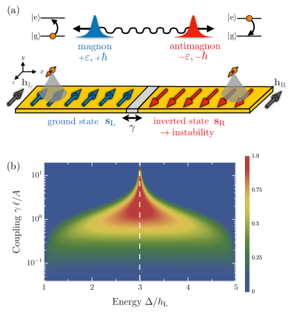
Figure 1: (a) Setup for magnon-antimagnon pair creation at the interface between two ferromagnets, one in the ground state (left) and one in the inverted state (right). The ferromagnets are magnetically coupled to color centers (orange arrows) that can absorb the generated magnon-antimagnon pairs and become entangled with each other. (b) Steady-state concurrence ${\cal C}$ (an entanglement measure) as a function of the color center energy $\Delta$ and the interfacial coupling $\gamma$. We choose $h_{\text{R}}=5h_{\text{L}}$ and define the length scale $\ell=\sqrt{A/(h_{\text{R}}{-}h_{\text{L}})}$.

A necessary condition for creating steady-state entanglement between independent qubits that are weakly coupled through an environment is to drive the environment out of equilibrium. This is because in equilibrium — irrespective of how strong the environment correlations are — detailed balance will always enforce an uncorrelated Gibbs state [10]. Only transient entanglement generation may occur [7]. Therefore, we consider in this Letter the nonequilibrium magnetic environment shown in Fig. 1(a), which was studied in Ref. [11] as a magnonic version of the bosonic Klein paradox [12, 13]. A ground-state ferromagnet (left) is weakly coupled at the interface to an inverted-state ferromagnet (right), where the former is aligned and the latter is antialigned with the applied magnetic field. To avoid the instability, the inverted system is dynamically stabilized by a spin torque [11].

Conceptually, the physics is similar to an analog black hole [14, 15], where the horizon is mimicked by the interface between the stable and the unstable magnet with positive and negative excitation energies, respectively. Due to quantum fluctuations, this instability can be harvested through magnon pair production that is reminiscent of Hawking radiation. Here, the pair creation sustains a purely quantum spin current consisting of positive-energy magnons with $+\hbar$ emitted to the left and negative-energy magnons (or antimagnons [16]) with $-\hbar$ emitted to the right.

Our main result is demonstrating that two color centers, placed in proximity of the two magnets, pick up the entanglement of the magnon-antimagnon pairs in the nonequilibrium steady state. The anisotropic magnetostatic coupling between the dipole moments of the color centers and the stray field of the magnets turns out to be beneficial, as it facilitates a perfectly chiral coupling and eliminates dephasing. We derive a Lindblad master equation with nonlocal gain and loss and find that in the steady state, the color centers become entangled, see Fig. 1(b). The concurrence ${\cal C}$ [17], used as a measure of entanglement, is close to one in a sweet spot (red) tuned by the color center energy $\Delta$ and the weak interfacial exchange coupling strength $\gamma$. Along the symmetry axis (white dashed line), the steady state becomes pure and is of the simple form

$$\ket{\psi}=\frac{r\ket{\text{g,e}}-t\ket{\text{e,g}}}{\sqrt{{r}^{2}+{t}^{2}}},$$ (1)

where $g$ and $e$ denote the ground and the excited state of the two color centers.

Here, ${r}$ and ${t}$ are scattering amplitudes describing the pair creation in the environment (see details below). They are obtained from a generalized (nonunitary) scattering theory [14] using a bosonic Bogoliubov ansatz for both positive-energy and negative-energy magnons. The scattering amplitudes fulfill ${r}^{2}-{t}^{2}=1$. For zero interfacial coupling, $\gamma=0$, the production of magnon-antimagnon pairs is zero, which leads to ${t}=0$ and ${r}=1$. In this limit, we obtain the unentangled steady state $\ket{\psi}=\ket{\text{g,e}}$, where the spontaneous emission of a negative-energy magnon triggers a population inversion on the right side. As the coupling is turned on, $\gamma>0$, entangled magnon pairs are produced, ${t}>0$, and can nonlocally excite the color centers through dissipative coupling. In the limit ${r}\approx{t}\gg 1$, the steady state approaches the Bell state $\ket{\psi}\approx\left(\ket{\text{g,e}}-\ket{\text{e,g}}\right)/{\sqrt{2}}$.

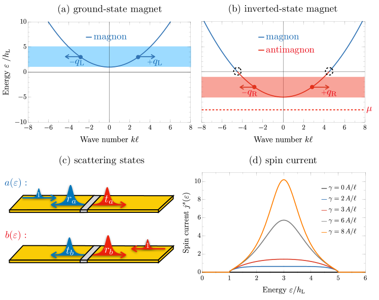
Figure 2: (a)-(b) Magnon excitation energies $\varepsilon_{\text{L,R}}$ for the left ground-state magnet (blue lines) and the right inverted-state magnet (red line). For energies $h_{\text{L}}<\varepsilon_{\text{L}}<h_{\text{R}}$ (blue area on the left) and $-h_{\text{R}}<{\varepsilon}<-h_{\text{L}}$ (red area on the right) magnons with positive and negative energy can be created pairwise at the interface. The dashed circles indicate the zero-energy magnons that potentially can induce dephasing. (c) Sketch of the scattering states $a(\varepsilon)$ and ${b}(\varepsilon)$. (d) The magnon pair creation sustains a spin current $j^{s}(\varepsilon)$ in the vacuum state $\ket{\Omega}$, which is flowing to the left. The current is only nonzero for energies $h_{\text{L}}<\varepsilon<h_{\text{R}}$. The stronger the coupling $\gamma$ at the interface, the more pairs are emitted. The parameters are the same as in Fig. 1.

Nonequilibrium magnetic environment.—We model the nonequilibrium magnetic environment via the Hamiltonian $H_{\text{E}}=\int\mathrm{d}x\left({\cal H}_{\text{L}}+{\cal H}_{\text{R}}+{\cal H}_{\text{I}}\right)$ that consists of contributions from the left ground-state ferromagnet, the right inverted-state ferromagnet, and the coupling at the interface (see Fig. 1). In the absence of ${\cal H}_{\text{I}}$, the spin density $\mathbf{s}_{\text{L}}$ of the left side is in the ground state, $\expectationvalue{\mathbf{s}_{\text{L}}}=-s\mathbf{e}_{z}$, aligned with the external field $\mathbf{h}_{\text{L}}=-{h}_{\text{L}}\mathbf{e}_{z}/\hbar$, where $s$ is the spin density per length. On the right side, the spin density $\mathbf{s}_{\text{R}}$ is in the inverted state, $\expectationvalue{\mathbf{s}_{\text{R}}}=+s\mathbf{e}_{z}$, antialigned with the external field $\mathbf{h}_{\text{R}}=-{h}_{\text{R}}\mathbf{e}_{z}/\hbar$. This inverted state is unstable, since dissipation through Gilbert damping will relax the magnet to its ground state. A dynamical stabilization is achieved, for example, by pumping the inverted magnet through spin torques with a spin accumulation $\mu<-h_{\text{R}}$ below the magnon band [see red dashed line in Fig. 2(b)].

The degrees of freedom of this environment are captured by the magnonic field operators $\psi_{\text{L}}$ and $\psi_{\text{R}}$ with spin $+\hbar$ and $-\hbar$ on top of the ground ($x<0$) and the inverted state ($x>0$), respectively. They are defined via the usual linearized Holstein-Primakoff relations $\sqrt{2\hbar s}\psi_{\text{L}}\approx s_{\text{L}}^{x}-is^{y}_{\text{L}}$ and $\sqrt{2\hbar s}\psi_{\text{R}}\approx s_{\text{R}}^{x}+is^{y}_{\text{R}}$. Their dynamics in the bulk are described by the Hamiltonians

$${\cal H}_{\alpha}=A\left(\partial_{x}\psi^{\dagger}_{\alpha}\right)\left(\partial_{x}\psi_{\alpha}\right)\pm{h}_{\alpha}\psi^{\dagger}_{\alpha}\psi_{\alpha},$$ (2)

where $\alpha\in\text{L,R}$. The first term reflects the bulk exchange interaction with spin stiffness $A$ that favors a parallel alignment of the spins. The second term is the Zeeman energy. The resulting bulk excitation energies of the magnons are given by $\varepsilon_{\text{L,R}}=Ak^{2}\pm h_{\text{L,R}}$ (see blue lines in Fig. 2) as a function of the wavenumber $k$. The magnon energies are raised by $h_{\text{L}}$ in the left magnet, while they are lowered by $h_{\text{R}}$ in the right magnet. As a result, we obtain negative excitation energies, $\varepsilon_{\text{R}}<0$, which indicates the instability of the inverted magnet.

Generation of entangled magnon-antimagnon pairs occurs when the inverted magnet — which acts as a source of energy — is coupled at the interface to the normal magnet. We assume an exchange coupling $\sim\mathbf{s}_{\text{L}}\cdot\mathbf{s}_{\text{R}}$ that couples the left and right magnons via

$${\cal H}_{\text{I}}=\gamma\delta(x)\left(\psi_{\text{L}}^{\dagger}\psi_{\text{L}}+{\psi}_{\text{R}}^{\dagger}{\psi}_{\text{R}}+{\psi}_{\text{R}}\psi_{\text{L}}+\psi_{\text{L}}^{\dagger}{\psi}_{\text{R}}^{\dagger}\right),$$ (3)

where $\gamma$ is the exchange coupling strength. In a linear treatment of the spin fluctuations, the sign of $\gamma$ is irrelevant. Also, we are interested in the regime of a weak link, where the microscopic exchange energy is much weaker at the interface than in the bulk. Crucially, ${\cal H}_{\text{I}}$ contains the pair creation term $\sim\delta(x)\psi_{\text{L}}^{\dagger}\psi_{\text{R}}^{\dagger}$ that becomes resonant when positive-energy magnons in the left magnet [blue filled dots in Fig. 2(a)] are matched with negative-energy magnons in the right magnet [red dots in Fig. 2(b)]. This can only happen for energies in the interval $h_{\text{L}}<\varepsilon_{\text{L}}<h_{\text{R}}$ (blue shaded area) and $-h_{\text{R}}<\varepsilon_{\text{R}}<-h_{\text{L}}$ (red shaded area). Thus, we require $h_{\text{R}}-h_{\text{L}}>0$. The last two terms of Eq. (3) generate two-mode squeezing similar to photon pair creation in parametric amplifiers [18, 19].

Magnon-antimagnon pair creation.—Production of entangled magnon-antimagnon pairs is described by a generalized (nonunitary) scattering theory in a bosonic Bogoliubov space. The calculations are performed in analogy to Ref. [14], where Hawking radiation of phonons in acoustic black holes is investigated. Expanding the magnon field operators in terms of in-scattering states, we obtain [20]

$$\psi_{\text{L}}(x) =\int\limits_{h_{\text{L}}}^{h_{\text{R}}}\frac{\mathrm{d}\varepsilon}{\sqrt{hv_{\text{L}}}}\Bigg{[}\left(e^{iq_{\text{L}}x}{+}r_{a}e^{{-}iq_{\text{L}}x}\right)a_{\varepsilon}+{t}_{b}e^{{-}iq_{\text{L}}x}b_{-\varepsilon}^{\dagger}\Bigg{]},$$

$${\psi}_{\text{R}}(x) =\int\limits_{-h_{\text{R}}}^{-h_{\text{L}}}\frac{\mathrm{d}\varepsilon}{\sqrt{h{v}_{\text{R}}}}\Bigg{[}\left(e^{-i{q}_{\text{R}}x}{+}{r_{b}}e^{i{q}_{\text{R}}x}\right)b_{\varepsilon}{+}t_{a}e^{i{q}_{\text{R}}x}{a}_{{-}\varepsilon}^{\dagger}\Bigg{]},$$ (4)

where $h=2\pi\hbar$ is the Planck constant. The operators $a_{\varepsilon}$ and $b_{\varepsilon}$ describe the two relevant in-scattering solutions with $\left[a_{\varepsilon},a^{\dagger}_{\varepsilon^{\prime}}\right]=\left[b_{\varepsilon},b^{\dagger}_{\varepsilon^{\prime}}\right]=\delta(\varepsilon{-}\varepsilon^{\prime})$ [see Fig. 2(a)-(c)]. The scattering mode $a_{\varepsilon}$ describes an incident positive-energy magnon from the left with amplitude one that gets reflected with amplitude $r_{a}(\varepsilon)$ and transmitted as a negative-energy magnon with amplitude $t_{a}(\varepsilon)$ [see Fig. 2(c)]. Scattering into positive-energy magnons on the right is not allowed by spin conservation. Similarly, the scattering mode ${b}_{\varepsilon}$ describes an incident negative-energy magnon from the right with amplitude one that gets reflected with amplitude $r_{b}(\varepsilon)$ and transmitted as a positive-energy magnon with amplitude ${t}_{b}(\varepsilon)$ [see Fig. 2(c)]. The wave numbers are given by $q_{\text{L}}=\sqrt{(\varepsilon{-}h_{\text{L}})/A}$ and $q_{\text{R}}=\sqrt{(\varepsilon{+}h_{\text{R}})/A}$ with group velocities $v_{\text{L}}=2Aq_{\text{L}}/\hbar$ and ${v}_{\text{R}}=2Aq_{\text{R}}/\hbar$, respectively. We remark that the expansion from Eq. (4) is incomplete as higher-energy scattering solutions are omitted. These scattering states are irrelevant for our findings below but are fully accounted for in the Supplemental Material [20], where we also give the specific form of the scattering amplitudes.

The scattering amplitudes from Eq. (4) can be compactly encoded in the scattering matrix:

$$S=\begin{pmatrix}r_{a}(\varepsilon)&&{t}_{b}(\varepsilon)\\ t_{a}^{*}(-\varepsilon)&&{r}_{b}^{*}(-\varepsilon)\end{pmatrix},$$ (5)

where $S$ relates the in-scattering states $(a_{\varepsilon},b_{-\varepsilon}^{\dagger})$ to their corresponding out-scattering counterparts. The full energy dependence of $S$ is determined from the matching conditions at the interface described by Eq. (3). Importantly, the scattering matrix is not unitary but fulfills $S\tau_{z}S^{\dagger}=\tau_{z}$ with Pauli matrix $\tau_{z}$ in order to maintain the bosonic commutaion relations of $a_{\varepsilon}$ and $b_{-\varepsilon}^{\dagger}$. In addition, there exists an effective time reversal symmetry $SS^{*}=\mathds{1}$. It directly follows that $\absolutevalue{{t}_{a}(-\varepsilon)}=\absolutevalue{{t}_{b}(\varepsilon)}\equiv t$, $\absolutevalue{{r}_{a}(\varepsilon)}=\absolutevalue{{r}_{b}(-\varepsilon)}\equiv r$, as well as ${r}^{2}-{t}^{2}=1$. The last relation lies at the heart of the bosonic Klein paradox [12, 13], where the nonunitarity of $S$ can enhance both the reflection and the transmission amplitudes, ${r}>{t}>1$. In contrast, for conventional scattering problems, unitarity enforces ${r}^{2}+{t}^{2}=1$.

Having solved for the magnon operators, we can determine the spin current due to the spontaneous pair production via

$${\hat{I}}^{s}_{\alpha}(x)=\pm 2A\left[{\psi}_{\alpha}^{\dagger}\left(-i\partial_{x}{\psi}_{\alpha}\right)-\left(-i\partial_{x}\psi_{\alpha}^{\dagger}\right){\psi}_{\alpha}\right],$$ (6)

where the $+$ and the $-$ sign holds for $\alpha=\text{L}$ and $\alpha=\text{R}$, respectively. Even in the vacuum state defined through

$$a(\varepsilon)\ket{\Omega}={b}(\varepsilon)\ket{\Omega}=0,$$ (7)

the system sustains a spin current that is flowing to the left:

$$\expectationvalue{{\hat{I}}^{s}_{\alpha}(x)}{\Omega}=-\frac{1}{\pi}\int\limits_{h_{\text{L}}}^{h_{\text{R}}}{\mathrm{d}\varepsilon}\,t(\varepsilon)^{2}.$$ (8)

Here, the prefactor follows from $2\hbar/h$, where each magnon carries the spin $\hbar$, in analogy to the electron current in the Landauer-Büttiker formalism [21]. The spin current is purely quantum as it originates in the vacuum fluctuations at the interface. It only flows in the energy window $h_{\text{L}}<\varepsilon<h_{\text{R}}$ and it corresponds to the constant creation of magnon-antimagnon pairs, where $+\hbar$ magnons with positive energy move to the left and $-\hbar$ magnons with negative energy (or antimagnons) move to the right. In Fig. 2(d), we show the energy-resolved spin current $j^{s}(\varepsilon)=\,t^{2}/\pi$ as a measure of the spontaneous pair emission spectrum. The emission occurs symmetrically with respect to $\varepsilon=(h_{\text{L}}{+}h_{\text{R}})/2$. A significant change of the spin current $j^{s}$ occurs as the exchange coupling $\gamma$ is varied on the characteristic scale ${A/\ell}$ with $\ell=\sqrt{A/(h_{\text{R}}{-}h_{\text{L}})}$. In a microscopic Heisenberg model, this characteristic value $\gamma\sim{A/\ell}$ translates to $J^{\prime}\ell\sim Ja$, where $J$ and $J^{\prime}$ are the bulk and interfacial exchange energies and $a$ is the atomic lattice constant. Since $\ell\gg a$, a weak link with $J^{\prime}\ll J$ is sufficient to enable spontaneous pair emission with $j^{s}\sim{\cal O}(1)$. In a recent work [22], the current-current correlations were analyzed to investigate the entanglement between magnons and antimagnons.

Imprinting entanglement.—To sense the pair creation, we couple two color centers to the magnet. Their bare Hamiltonian is given by $H_{\text{S}}=-\Delta\sigma^{z}_{\text{L}}/2-\Delta\sigma^{z}_{\text{R}}/2$, with $\Delta>0$, using the Pauli matrices $\sigma_{\alpha}^{j}$ labeled by $j\in x,y,z$. Thus, energetically both color centers favor the $+z$ direction, with ground state $\ket{\text{g,g}}$. The basis states are denoted by $\ket{\text{g,g}},\ket{\text{g,e}},\ket{\text{e,g}}$ and $\ket{\text{e,e}}$ with g and e standing for the ground and the excited state, respectively.

The color centers interact with the stray field $\mathbf{h}_{s}$ of the environment through the magnetostatic coupling Hamiltonian

$$H_{\text{C}}=-\frac{\hbar}{2}\sum\limits_{\alpha=\text{L,R}}\Bigg{[}h^{+}_{s}(\mathbf{r}_{\alpha})\sigma^{-}_{\alpha} +h^{-}_{s}(\mathbf{r}_{\alpha})\sigma^{+}_{\alpha}+h^{z}_{s}(\mathbf{r}_{\alpha})\sigma_{\alpha}^{z}\Bigg{]},$$ (9)

where we introduced $\sigma_{\alpha}^{\pm}=\left(\sigma^{x}_{\alpha}\pm i\sigma^{y}_{\alpha}\right)/2$ and $h_{s}^{\pm}=h^{x}_{s}\pm ih^{y}_{s}$. Here, $\mathbf{r}_{\alpha}=(x_{\alpha},d,0)$ denotes the position of the color centers at height $d>0$ on either side of the interface with $x_{\text{L}}<0$ and $x_{\text{R}}>0$ (see Fig. 1). The stray field $\mathbf{h}_{s}$ can be calculated via the magnetostatic Greens function [23], where its source are the magnonic excitations described by $\psi_{\text{L}}$ and ${\psi}_{\text{R}}$ of Eq. (4).

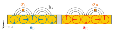
Figure 3: Snapshot of Halbach-like stray field $\mathbf{h}_{s}$ from the magnetic excitations described by $\mathbf{s}_{\text{L}}$ and $\mathbf{s}_{\text{R}}$. The stray magnetic field is only created above the magnet if magnons are moving to the left (right) on the left (right) side. In addition, a combination of time reversal symmetry and mirror symmetry in the $xy$ plane ensures $h_{s}^{z}=0$.

Generically, the anisotropy of the magnetostatic coupling from Eq. (9) is expected to be a nuisance, as it spoils the spin $z$ symmetry and can lead to magnon-induced dephasing [which is resonant at zero energy and therefore energetically enabled by the instability in the right magnet, see dashed circles in Fig. 2(b)]. However, in our setup, the coupling turns out to be beneficial for two reasons. First, due to a combination of time-reversal and $xy$ mirror symmetry of the magnonic spin excitations (see Fig. 3), it follows that $h_{s}^{z}=0$. This eliminates magnon-induced dephasing of the color centers. Second, as shown in Fig. 3, the stray field of a single magnon is Halbach array-like [24], so it is nonzero either only above or below the magnet depending on its wave vector $k$. In order to be sensitive to the pair creation, we want the left color center to couple to left-moving positive-energy magnons ($k=-q_{\text{L}}$) and the right color center to couple to right-moving negative-energy magnons ($k=+{q}_{\text{R}}$). For $\absolutevalue{x_{\alpha}}\gg d$, we obtain [20]

$$h^{+}_{s}(\mathbf{r}_{\text{L}}) \propto\int\limits_{h_{\text{L}}}^{h_{\text{R}}}\frac{\mathrm{d}\varepsilon}{\sqrt{hv_{\text{L}}}}q_{\text{L}}e^{-q_{\text{L}}d}e^{-iq_{\text{L}}x_{\text{L}}}\Bigg{(}r_{a}a_{\varepsilon}+{t}_{b}{b_{-\varepsilon}^{\dagger}}\Bigg{)},$$ (10)

$$h^{-}_{s}(\mathbf{r}_{\text{R}}) \propto\int\limits_{-h_{\text{R}}}^{-h_{\text{L}}}\frac{\mathrm{d}\varepsilon}{\sqrt{h{v}_{\text{R}}}}{q}_{\text{R}}e^{-{q}_{\text{R}}d}e^{i{q}_{\text{R}}x_{\text{R}}}\Bigg{(}r_{b}b_{\varepsilon}+{t}_{a}a^{\dagger}_{-\varepsilon}\Bigg{)}.$$ (11)

Thus, the dipole coupling has introduced the typical filter function $q_{\text{L}}e^{-q_{\text{L}}d}$ and ${q}_{\text{R}}e^{-{q}_{\text{R}}d}$ [25, 23]. In addition, the chirality has eliminated the incoming plane waves with amplitude one from Eq. (4).

Integrating out the environment degrees of freedom $a_{\varepsilon}$ and ${b}_{\varepsilon}$ in the effective vacuum state $\ket{\Omega}$, we obtain a Lindblad master equation for the reduced density matrix $\rho$ in a Born-Markov treatment [20]

$$\partial_{t}\rho=\frac{1}{i\hbar}\left[H_{\text{S}}+\delta H,\rho\right]+\sum_{i=1}^{2}\Gamma_{0}\left(L_{i}\rho L_{i}^{\dagger}-\frac{1}{2}\{L^{\dagger}_{i}L_{i},\rho\}\right),$$ (12)

where the rate is given by $\Gamma_{0}=\gamma_{e}^{4}\hbar^{2}s/W^{2}Ad$ in Gaussian units with the gyromagnetic ratio $\gamma_{e}$ and the width of the magnetic strip $W$. The magnetic fluctuations encoded in Greens functions of $h^{+}_{s}(\mathbf{r}_{\alpha})$ and $h^{-}_{s}(\mathbf{r}_{\alpha})$ generically induce both nonlocal coherent dynamics described by $\delta H$ as well as nonlocal dissipative dynamics described by the Lindblad operators $L_{1}$ and $L_{2}$. By using the properties $S\tau_{z}S^{\dagger}=\tau_{z}$ and $SS^{*}=\mathds{1}$ of the nonunitary scattering matrix, it can be shown that $\delta H=0$ . For the nonlocal dissipation, we obtain the Lindblad operators

$$L_{1} =\sqrt{q_{\text{L}}d}\,e^{-q_{\text{L}}d}r\,{\sigma}^{+}_{\text{L}}+\sqrt{\bar{q}_{\text{R}}d}\,e^{-\bar{q}_{\text{R}}d}t\,{\sigma}^{+}_{\text{R}},$$ (13)

$$L_{2} =\sqrt{q_{\text{L}}d}\,e^{-q_{\text{L}}d}t\,{\sigma}^{-}_{\text{L}}+\sqrt{\bar{q}_{\text{R}}d}\,e^{-\bar{q}_{\text{R}}d}r\,{\sigma}^{-}_{\text{R}},$$ (14)

where all functions are evaluated at the resonant energy $\varepsilon=\Delta$ and we define $\bar{q}_{\text{R}}(\Delta)={q}_{\text{R}}(-\Delta)$. In addition, we performed local $z$ rotations to obtain the real amplitudes $r$ and $t$. The dependence on the positions of the color centers $x_{\alpha}$ has disappeared due to the chiral nature of the coupling.

The Lindblad operator $L_{1}$ ($L_{2}$) describes the emission (absorption) of a positive-energy magnon on the left side paired with the absorption (emission) of a negative-energy magnon on the right side, with both processes decreasing (increasing) the energy of the color centers. In the limit of no pair creation, $\gamma\rightarrow 0$, we obtain $r=1$ and $t=0$. Then, $L_{1}$ and $L_{2}$ trigger the spontaneous emission of a positive-energy magnon on the left side and a negative-energy on the right side. Thus, the steady state of the color centers becomes $\ket{g,e}$, where on the right side a population inversion is created akin to negative temperature. For finite coupling, $\gamma>0$, magnon-antimagnon pairs are produced, which enables both absorption with $t>0$ and stimulated emission with $r>1$. Then, the environment can imprint entanglement by admixing the $\ket{e,g}$ state. In Fig. 1(b), we show the concurrence ${\cal C}$ of the steady state that follows from Eq. (12). For zero coupling, $\gamma=0$, we get ${\cal C}=0$, as the steady state is $\ket{g,e}$. However, as the coupling $\gamma$ is turned on, entanglement is created and we observe a sweet spot [red in Fig. 1(b)] with a concurrence close to one, where the interfacial coupling is at around $\gamma\sim\sqrt{A(h_{\text{R}}{-}h_{\text{L}})}$ and $\Delta\sim(h_{\text{L}}{+}h_{\text{R}})/2$. As $\gamma$ increases beyond the sweet spot, the pair creation appears more classical and entanglement only occurs in a narrow window around $\Delta=(h_{\text{L}}{+}h_{\text{R}})/2$. At this tuned position we obtain $q_{\text{L}}=\bar{q}_{\text{R}}$ and the steady state becomes pure and has a particularly simple form given by Eq. (1). The concurrence in this case reduces to ${\cal C}=2rt/({r}^{2}{+}{t}^{2})$. We remark that the chiral nature of the coupling is not essential to create entanglement. Without chirality, the spatial dependence of the scattering solution would survive [20].

Conclusion.—In this Letter, we demonstrated that steady-state entanglement can be imprinted onto a pair of color centers by letting them weakly interact with a magnetic solid-state environment. A necessary ingredient is to drive the environment out of equilibrium, which is achieved by an inverted magnet that can host negative-energy magnons (or antimagnons). At the interface to a normal magnet, positive-energy and negative-energy magnons are created in entangled pairs. Via a chiral magnetostatic coupling to the stray field of the magnet, the two color centers can pick up the magnon-antimagnon pairs through nonlocal absorption and emission processes. In a sweet spot, tuned by the color center energy and the interfacial exchange coupling, the color centers naturally evolve into an entangled steady state that even approaches the Bell state.

A key to imprinting entanglement was the creation of two-mode squeezing between positive-energy and negative-energy magnons. We emphasize that rather than an external drive, the interfacial exchange coupling served as an outlet that can harvest the energy supplied by the bulk inverted magnet. This is contrasted with the parametric drive used to create squeezing in quantum optics [27, 18, 19].

For future work, it might be interesting to embrace the full nonlinearity of the spin dynamics in the environment in order to prepare non-Gaussian states, going beyond two-mode squeezing. Furthermore, it seems promising to couple different magnetic systems to the inverted region that can be used as a source of energy to induce interesting entangled dynamics. Yet another promising route is to scale up the effect by considering two-dimensional generalizations, which allows an extended ensemble of color centers placed at interfaces between ground- and inverted-state regions.