Masked Image Contrastive Learning for Efficient Visual Conceptual Pre-training

Abstract

This paper proposes a scalable and straightforward pre-training paradigm for efficient visual conceptual representation called masked image contrastive learning (MiCL). Our MiCL approach is simple: we randomly mask patches to generate different views within an image and contrast them among a mini-batch of images. The core idea behind MiCL consists of two designs. First, masked tokens have the potential to significantly diminish the conceptual redundancy inherent in images, and create distinct views with substantial fine-grained differences on the semantic concept level instead of the instance level. Second, contrastive learning is adept at extracting high-level semantic conceptual features during the pre-training, circumventing the high-frequency interference and additional costs associated with image reconstruction. Importantly, MiCL learns highly semantic conceptual representations efficiently without relying on hand-crafted data augmentations or additional auxiliary modules. Empirically, MiCL demonstrates high scalability with Vision Transformers, as the ViT-L/16 can complete pre-training in 133 hours using only 4 A100 GPUs, achieving 85.8% accuracy in downstream fine-tuning tasks.

1 Introduction

Self-supervised learning (SSL) is considered the cornerstone towards building a world model, particularly in the pre-training of vision model [4, 12, 2, 19, 23, 28], attributed to its ability to acquire versatile visual representations without the need for human annotations. Currently, two dominant learning paradigms in visual self-supervised learning are the Masked Image Modeling (MIM) [12, 23, 17, 31, 11] and Contrastive Learning (CL) [4], exhibiting promising scalability characteristics for vision models, notably Vision Transformers (ViTs) [8].

Despite the success of these methods, both of these prevailing paradigms suffer from efficient visual representation, due to image sparsity and conceptual redundancy. The image sparsity leads to an excessive focus on local details during pixel-level reconstruction in MIM, rather than the highly semantical concepts. On the flip side, conceptual redundancies typically result in transformed images that fail to exhibit significant distinctions in CL. Hence, a pertinent question emerges: beyond the existing MIM and CL paradigms, how to reconcile the divergence between efficient visual representation and effective conceptual pre-training?

In elucidating this query, our initial step involves a revisit to the present pre-training paradigms, namely MIM and CL. Regarding MIM, it aims to learn visual representatives by reconstructing the masked image patches, as illustrated in Fig.1(b). Among these methods, BEiT [2] and MAE [12] are representatives. It is important to mention, that MAE indicates that there remains significant semantic redundancy within images, that only a small high-level understanding of parts, objects, and scenes is required to recover missing patches from neighbouring patches. However, pixel-level restoration is overly fine-grained for the pre-training of a vision model, excessively focusing on high frequencies and local details of the image. It runs counter to the core of pre-training, which is targeted at encapsulating high-hierarchical semantic image concepts. Despite this intricate task aids in the acquisition of visual representatives by the model, it regrettably fails to address concerns regarding pre-training efficiency.

In terms of CL, the underlying principle of it hinges on a quite simple concept: maximum agreement between varying views from a single image, as exhibited in Fig.1(a), where SimCLR [4, 5], MoCo v3 [6] and DINO [3] are typical representatives. Within this cohort, sophisticated pre-processing techniques and intricate auxiliary networks are required to capture distinct views of the image, thereby presenting a challenging task of optimizing the agreement among different views. Consequently, it can be derived that the essence of contrastive learning lies in the creation of distinct views characterized by substantial disparities. However, this endeavour presents a formidable challenge owing to the inherent conceptual redundancy prevalent in images. Moreover, large batch sizes are prerequisites for the generation of negative sample pairs, leading to a long training time and huge computing resources consumption.

Driven by this analysis, we found that these two paradigms can complement each other: masked tokens have the potential to significantly diminish the conceptual redundancy inherent in images, whereas contrastive learning is adept at extracting high-level semantic features during the pre-training phase. Thus, we present a novel and straightforward paradigm for self-supervised visual representation learning: masked image contrastive learning (MiCL). MiCL tackles the above issues systematically: I) Masked image tokens offer diverse views of a single image with substantial fine-grained conceptual differences. II) Contrastive learning enables pre-training to concentrate exclusively on the high-level semantic information contained within images while disregarding high-frequency redundancies. III) The proposed paradigm obviates the need for auxiliary modules and expedites the efficient extraction of model features.

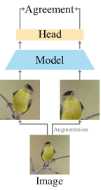
(a) Contrastive Learning

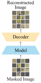
(b) Masked Image Modeling

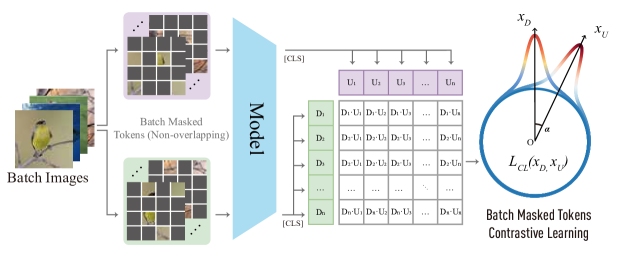
(c) Our Masked Image Contrastive Learning

Figure 1: Comparison between different pre-training paradigms. The Model in blue is the pre-training model, and the orange modules indicate auxiliary modules. (a) Contrastive Learning endeavours to maximize the agreement between different views of an image. (b) Masked Image Modeling aims to restore masked image patches. (c) Our Masked Image Contrastive Learning: Through non-overlapping masking, distinct tokens within an image are categorized as intraclass, while across-images tokens within a batch are viewed as interclass. Our objective is to enhance intraclass compactness and interclass separability through a contrastive learning approach. It is worth noting that our method does not necessitate any auxiliary modules, ensuring that no training resources are expended on redundant networks.

MiCL has a particularly simple and straightforward workflow, as presented in Fig.1(c). Here is how it works: Firstly, we mask a batch of images with a high rate, dividing visible patches within one image into two non-overlapping groups. In succession, the pre-train model extracts the features of these two groups of batch image tokens, respectively. Subsequently, contrastive learning is employed to predict the correct pairings for a batch of visible image tokens. Positive samples are different visible tokens in the same image, while negative samples are from different images of the mini-batch. Finally, inspired by T-distributed classifier [26, 27], we introduce the T-distributed spherical loss to constrains the inter-class margins in the pre-training. Comprehensive experiments demonstrate the scalability and efficacy of our approaches, where ViT-L/16 can complete pre-training in 133 hours using only 4 A100 GPUs and attain an 85.8% top-1 accuracy in fine-tuning classification. In particular, our model stands out from other pre-training methods as it operates without the need for auxiliary modules or hand-crafted data augmentation to generate diverse views.

In summary, our paper mainly makes the following contributions:

1. We endeavour to explore an alternative of using masked images to create diverse views with fine-grained conceptual differences for contrastive learning. By forgoing the conventional approach of employing instance-level hand-crafted data augmentation to generate distinct views, MiCL diminishes the conceptual redundancy inherent in images and improves efficiency.

2. Our approach eschews the reconstruction of masked images in favor of leveraging contrastive loss to steer the entire model. Independently of additional auxiliary modules, MiCL is adept at extracting high-level semantic concept features from images more efficiently.

3. Extensive experiments are conducted to verify the efficiency and scaling capability of our method. ViT-L/16 can complete pre-training in 133 hours using only 4 A100 GPUs with 85.8% accuracy in fine-tuning. Additionally, we have structured ablation experiments to delve into the implications of different configurations within MiCL, with a particular focus on the need of the MLP head in contrastive learning.

2 Related Works

2.1 Masked Image Modeling

Inspired by masked language modeling in NLP, the core of masked image modeling is to predict the masked part of the input image. Among them, BEiT [2] tokenizes image patches through the reconstruction of the individual image using dVAE, and then predicts the tokens of the masked patches to learn visual representation.

Similarly, MAE [12] utilizes a high masked ratio (75%) to corrupt the image and directly reconstruct the pixel-level masked image patches. Subsequently, numerous studies have referenced this paradigm for pre-training endeavours, including DropPos [23], U-MAE [31] and CAE [7]. DropPos [23] incorporates position reconstruction to bolster the spatial awareness of ViTs. U-MAE [31] introduces a uniformity loss as a regularization to the MAE loss to further encourage the feature consistency of the pre-training, and addresses the dimensional feature collapse. CAE [7] decouples the learning processes for image representation and pretext tasks, enabling the pre-trained model to prioritize image representation while disregarding the pretext task.

Additionally, following the successful implementation of MAE, its applicability has been extended to diverse disciplines, such as SiamMAE [11] and MR-MAE [9].

2.2 Contrastive Learning

Within this cohort, SimCLR [4] demands sophisticated pre-processing techniques to capture distinct views of the image, intending to present a challenging task to facilitate the acquisition of effective visual representations in pre-training. Meanwhile, large batch size is the prerequisite for the generation of negative sample pairs. Thereby, it requires a long training time and huge computing resources. Besides, DINO [3] utilizes student-teacher architecture to extract visual representation from different views. Moreover, MoCo v3 [6] applies momentum update to drive the auxiliary network. Consequently, it can be derived that the essence of contrastive learning lies in the creation of distinct views characterized by substantial disparities. However, this endeavour presents a formidable challenge owing to the inherent semantic redundancy prevalent in images. Besides, ConCL [24] generates distinct concepts through image cropping and leverages contrastive learning within a teacher-student framework to pre-train pathological images.

2.3 Combination between MIM and CL

There are also a lot of efforts to bridge the gap between mask image modeling and contrastive learning, where the integration of teacher-student models emerges as the prevailing approach. iBOT [33] employs the teacher-student network to independently encode the two augmented views, with the student network processing masked images. The objectives of MIM and CL are jointly trained for self-distillation. Likewise, MST [18] introduces a masked token strategy leveraging multi-head self-attention maps, which selectively mask the tokens of the student network based on the output self-attention map of the teacher network, ensuring vital foreground remains intact. Similarly, SiameseIM [21] employs a Siamese network featuring two branches. The online branch encodes the initial view and predicts the representation of the second view based on their relative positions. Meanwhile, the target branch generates the target by encoding the second view.

ccMIM [32] leverages a contrastive loss to aid the reconstruction task as a regularizer, facilitating the extraction of image-wide global information from both masked and unmasked patches. Likewise, ConMIM [29] produces simple intra-image inter-patch contrastive constraints as the sole learning objectives for masked patch prediction, and strengthens the denoising mechanism with asymmetric designs to improve the network pre-training. Similarly, I-JEPA [1] predicts the feature encoding of the contextual region via MIM, and employs contrastive learning to align the features of neighbouring regions at the feature level. Additionally, CoMAE [25] also applies CL to assist cross-modal MIM tasks. Besides, LGP [15] integrates MIM and CL in a sequential cascade manner: early layers are first trained under one MIM loss, on top of which latter layers continue to be trained under another CL loss.

3 Methodology

3.1 Architecture

With an input image $x_{i}\in\mathbb{R}^{H\times W\times C}$, it is reshaped into a sequence of 2D patches $x_{p}\in\mathbb{R}^{N\times(P^{2}\cdot C)}$, where $(H,W)$ denotes the original image resolution, $C$ is the number of channels, $P$ represents the patch size, and $N=HW/P^{2}$ indicates the number of patches. Subsequently, a linear projection is employed on $x_{p}$ to transform it into $D$ dimensions, yielding patch embeddings $x\in\mathbb{R}^{N\times D}$. Following the MoCo v3 [6], the linear projection is initialized using the Xavier uniform method and remains fixed throughout pre-training to mitigate potential instability in ViT caused by the large batch size. Thereafter, fixed position embeddings $p\in\mathbb{R}^{(N+1)\times D}$ are incorporated into the patch embeddings to preserve positional information, employing sinusoidal positional encoding.

After random masking patches, visible patches that retain the original image position information are divided into two non-overleaping groups: $x_{U}\in\mathbb{R}^{n\times D}$ and $x_{L}\in\mathbb{R}^{{n\times D}}$, where $n$ denotes the number of visible patches. Each group adds an independent [CLS] token $x_{cls}\in\mathbb{R}^{D}$ to aggregate the information of each group. Moreover, [CLS] tokens of each group will add the position embeddings $p_{0}$. In succession, ViT [8] is utilized as our encoder. $z_{U}=[x^{U}_{cls};x_{U}]\oplus p$ and $z_{L}=[x^{L}_{cls};x_{L}]\oplus p$ are the input of pre-training ViT, where $\oplus$ denotes element-wise plus, and $f(\cdot)$ represents the ViT. Consequently, image feature tokens extracted by ViT are symbolized as $y=f(z)$, where $y\in\mathbb{R}^{(n+1)\times D}$. Furthermore, we only preserve [CLS] tokens $y_{cls}\in\mathbf{R}^{D}$ of both groups for contrastive learning, as it aggregates the high-level semantic information of each image. It is noteworthy that, unlike existing methodologies, we abstain from employing auxiliary modules. This allows our model to more easily extract image features and reduce the consumption of computing resources.

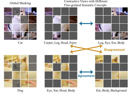
Figure 2: A toy example of masked images for conceptual contrastive learning. The low global masking ratio aids the model in capturing comprehensive information from the image and understanding the interconnectedness of various concepts within a mini-batch. Beyond that, each contrastive branch has a higher masking ratio, generating diverse views with different semantic concepts for contrastive learning and diminishing conceptual redundancy within the image.

3.2 Masked Image for Conceptual Pre-training

Despite the strides made in instance-wise contrastive learning [4, 3], the differences between various views primarily manifest at the pixel level, instead of semantic concept disparities. In this context, a patch is abstracted as a concept containing fine-grained semantics. The concepts within an image exhibit distinct conceptual characteristics, yet they are all interconnected with the overall meaning of the image, albeit to varying extents. Thus, masked images are used to create views that contain semantic distinctions of concepts, and mitigate the conceptual redundancy present in images, as presented in Fig. 2.

We apply the masking strategy of random sampling, the same as the MAE, which samples random patches without replacement following the uniform distribution. Beyond that, a low masking ratio (e.g. 30%) is implemented overall, but leads to a higher masking ratio (e.g. 65%) for individual contrastive branches, as illustrated in Fig. 2. The overarching low global masking rate facilitates the model in capturing the holistic information of the image and the interconnections among various concepts within a mini-batch. On the flip side, in each forward propagation, the model is exposed to a limited portion of the visible tokens, thereby generating diverse views with different fine-grained semantic concepts. The high masking ratio for each contrastive branch creates a pretext task that cannot be easily solved by extrapolation from simple image deformation, thus diminishing conceptual redundancy within the image, and emphasizing the localized features of the image. Furthermore, the masking strategy enables training solely on a few portions of the image, enhancing the scalability and efficiency of model training while accommodating the demands associated with large batch sizes in contrastive learning.

In terms of partitioning visible patches into two non-overlapping distinct groups, we simply employ a random sampling strategy akin to the aforementioned masking approach to mitigate potential biases, ensuring that the central positions of visible patches within the two groups remain consistent. Meanwhile, non-overlapping patches present a challenging scenario, impeding the model from relying solely on analogous patches for inference.

3.3 Efficient Contrastive Learning

We randomly select a mini-batch of $B$ instances and establish the contrastive prediction task on the visible token pairs extracted from this mini-batch, yielding a total of $2\times B$ data points. We designate feature tokens stemming from disparate groups within the same image as positive pairs. Conversely, tokens from distinct images within the same mini-batch are regarded as negative pairs. We concurrently maximise the similarity of $B$ positive pairs while minimizing the similarity of $B^{2}-B$ negative examples to drive the network.

In terms of similarity computation, we introduce T-distributed spherical (T-SP) metric [26, 16] to significantly promote the intraclass compactness and interclass separability of features. Given [CLS] tokens $y_{i}^{U}\in\mathbf{R}^{D}$ and $y_{j}^{L}\in\mathbf{R}^{D}$ of both non-overlapping groups, the cosine distances between $y_{i}^{U}$ and $y_{j}^{L}$ are:

$$cos_{LU}(y_{i}^{U},y_{j}^{L})=\frac{{y_{i}^{U}}^{T}y_{j}^{L}}{|y_{i}^{U}||y_{j}^{L}|}$$ (1)

and the T-SP similarity is defined as follows:

$$\text{sim}_{tsp}(y_{i}^{U},y_{j}^{L})=0.5\times\frac{1+cos_{LU}}{1+(1-cos_{LU})*\kappa}$$ (2)

where $\kappa\geq 0$ denotes the concentration hyperparameter of T-SP metric. As $\kappa$ decreases, the similarity function becomes more condensed, where only two tokens in close proximity are deemed positive examples. Besides, we add a trainable temputare parameter $\tau$ to effectively scale the different samples. Thus, the loss function for a positive pair is:

$$\mathcal{L}(y_{i}^{U},y_{j}^{L})$$ (3)

$$= -\log{\frac{\exp{(\text{sim}_{tsp}(y_{i}^{U},y_{j}^{L})\times\tau)}}{\sum_{k=1}^{2B}{\mathbbm{1}_{\left[k\neq i\right]}\exp{(\text{sim}_{tsp}(y_{i}^{U},y_{k}^{L})\times\tau)}}}}$$

where $\mathbbm{1}_{\left[k\neq j\right]}\in\{0,1\}$ is an indicator function evaluating to 1 if $k\neq i$. Finally, inspired by CLIP [19], we optimize a symmetric loss over these similarity scores within a mini-batch exhibited in Algorithm 1.

3.4 Simple implementation

# x[B,N,D] - patch embeddings

# mask image and split into two non-overleaping groups

# x [B$\times$2, n, L]

x = masking(x, ratio = 0.3)

# extract [CLS] token of both groups using pre-training model

x = model(x) # [B$\times$2, 1, L]

x = x.reshape(-1, 2, x.shape[-1])

# L2 normalize the [CLS] token of each group

m, n = x[:,0], x[:,1] # [B, L]

m = m/m.norm(dim=-1,keepdim=True)

n = n/n.norm(dim=-1,keepdim=True)

# compute the scaled pairwise T-SP similarities

sim_mn = compute_tSP(m @ n.T)

sim_nm = compute_tSP(n @ m.T)

# symmetric loss function

labels = torch.arange(B)

loss=(F.cross_entropy(sim_mn,labels) +F.cross_entropy(sim_nm,labels))/2

Algorithm 1 Pytorch-like pseudo code for the core of an implement of MiCL

The implementation of our MiCL pre-training is efficient and involves minimal specialized operations. As pseudo code depicted in Algorithm 1, we make only minor modifications based on the MAE code, mainly involving the process subsequent to the acquisition of image feature embeddings from the encoder. First, we randomly mask a subset of embedded patch tokens with a low masking ratio. In succession, listed tokens are shuffled randomly and divided into two non-overlapping groups. Following MAE [12], within positional and [CLS] embeddings, lists of tokens are encoded by the ViT. It is noteworthy that we obtain the encoded [CLS] token from the ViT directly, without the incorporation of additional auxiliary modules, even a linear head or lightweight decoder.

Subsequently, the obtained [CLS] tokens within each group are L2 normalized, and then the T-SP metric is applied to calculate the similarity between tokens from each group. Finally, a simple cross-entropy loss is calculated symmetrically to drive model training, enhancing the intraclass conceptual compactness within an image and the interclass semantic separability across images.

4 Experiments

Model	Blocks	Dim	Heads	Params
ViT-B/16 [8]	12	768	12	86M
ViT-L/16 [8]	24	1024	16	304M
ViT-h/16 [8]	32	1280	16	632M

Table 1: Configurations of Vision Transformer models in our experiments. Block denotes the number of transformer blocks, with dim representing the dimension of the input/output channel dimension of all blocks. Heads are the number of heads in multi-head attention modules. And we also provide the parameter sizes of different models.

We conduct self-supervised pre-training on the ImageNet-1K [20] dataset with the resolution of 224$\times$224. By default, ViT-B/16 and ViT-L/16 [8] are leveraged as the backbone architecture with 800 epochs for pre-training and 40 epochs for warm-up. ViT-B/16 applies the overall masked ratio of 0.3, while ViT-L/16 is set to 0.4. And the initial base learning rate is $1.5\times 10^{-4}$. Similar to other contrastive learning [4, 19], our method relies on the large effective batch size, specifically set at 9,600 for ViT-B/16 and 2,048 for ViT-L/16. Besides, $\kappa$ is set to 64 in the T-SP metric to compute the similarity by default. Our implementation is based on MAE [12]. Details can be found in Supplementary Material.

In terms of supervised validation, MiCL is evaluated through end-to-end fine-tuning and linear probing on the ImageNet-1k dataset for classification with 100 epochs for ViT-B/16 and 50 for ViT-L/16, following common practices [3, 12, 23]. Top-1 accuracy is utilized to verify the performance of different methods.

4.1 Scalability

To demonstrate the scalability of our MiCL for efficient conceptual pre-training, we access the efficiency and scaling of our model in Fig.3. It illustrates the pre-training hours related to various model sizes for different methods, with linear probing accuracy.

Figure 3: Efficiency and Scaling. MAE [12], I-JEPA [1] and MoCo v3 [6] are opted for comparison. All methods are evaluated by linear probing with Top-1 accuracy (Acc) as the metric, and the pre-training GPU time with A100 hour as the indicator. The pre-training epochs (denoted as ep) and model architecture are also exhibited.

Model Efficiency. MiCL presents highly scalable in contrast to prior methodologies, demanding reduced computational resources while delivering exemplary results, without relying on handcrafted data augmentations. Compared to reconstruction-based methods, such as MAE and I-JEPA, we necessitate fewer epochs and omit the need for context pixel-level reconstruction, thus resulting in significantly improved speed. On the flip side, concerning contrastive learning methods like MoCo v3 which rely on hand-crafted data augmentations for generating and processing multiple image views, MiCL dispenses with auxiliary modules like the momentum encoder akin to MoCo v3. The simple and straightforward framework of MiCL accelerates the pre-training. In particular, when the model becomes larger from ViT-B/16 to ViT-L/16, additional pre-training time is far away less than the MoCo v3.

Scaling model size. Moreover, our model leverages a scalable model size, resulting in more substantial performance enhancements with the larger model as illustrated in Fig.3. Compared to ViT-B/16, MiCL achieves nearly 4% improvement in linear probing with ViT-L/16, surpassing MoCo v3. It implies that we can efficiently train larger models to achieve better performance, within an acceptable timeframe.

4.2 Ablation Studies

4.2.1 Masked Ratio

Overall Masked Ratio	Forward Visible Ratio	Eff. Bsz.	LIN	FT
ViT-L/16
0.2	0.4	1,024	74.2	84.4
0.4	0.3	2,048	77.9	85.8
0.8	0.1	7,200	69.1	83.0
ViT-B/16
0.3	0.35	9,600	74.2	83.4
0.6	0.2	9,600	71.0	82.8
0.8	0.1	12,800	65.7	81.6

Table 2: Ablation evaluation experiments on masked ratio. The results are based on the ImageNet-1K with the Vit-B/16 and ViT-L/16. All methods are evaluated by linear probing (LIN) and fine-tuning (FT). We provide the visible ratio of each branch for contrastive learning according to the masked ratio. Correspondingly, we give different effective batch sizes (Eff. Bsz.) related to the overall masked ratio. The resolution of images is fixed to 224×224. Top-1 accuracy is used as the metric.

Firstly, we conduct ablation experiments to discuss the impact of the overall masked ratio on the performance of conceptual pre-training, revealed in Table 2. To ensure clarity in presentation, we offer the visible ratio of each contrastive branch within a single forward pass of the mini-batch, which is a crucial factor for the cross-similarity within our MiCL framework. Likewise, the effective batch size is intertwined with the scalable masked ratios, with larger batch sizes showcasing performance enhancements for the model, as verified in Section 4.2.2. Thus, we attribute this improvement to the masked ratio.

Regarding large models such as ViT-L/16 in Table 2, the increment of the overall masked ratio from 0.2 to 0.4 could significantly diminish conceptual redundancy and increase the effective batch size, thereby resulting in performance improvement. Nevertheless, with a continued rise in the masked ratio, the visible patches of images in one forward process of the model diminish incrementally. Despite increases in batch size, the precise extraction of conceptual information from the images becomes compromised, resulting in degraded performance. Furthermore, as displayed in ViT-B/16 of Table 2, once the batch size surpasses its threshold, an excessively high masked ratio can impair the model performance, transitioning from reducing conceptual redundancy to damaging essential semantic information.

4.2.2 Large Batch Size for Contrastive Learning

Act. Bsz.	Eff. Bsz.	LIN	FT	Pre-training Hour
512	2,048	77.9	85.8	533
512	4,096	77.7	85.7	533
450	1,800	77.4	85.7	559
256	1,024	74.4	84.9	586
128	512	71.6	84.6	613

Table 3: Ablation evaluation experiments on batch size. The results are based on the ImageNet-1K with the ViT-L/16. All methods are evaluated by pre-training hours, linear probing (LIN) and fine-tuning (FT). Different from other methods, MiCL is very dependent on the size of the mini-batch (denoted as Act. Bsz.), instead of effective batch size (denoted as Eff. Bsz.). So, we offer both parameters of batch size. Besides, pre-training hours on A100 are provided. The resolution of images is fixed to 224×224. Top-1 accuracy is used as the metric.

ViT models [8] are inherently computationally intensive, and training with large batches is a preferred strategy for handling large ViT models. Moreover, a sizable batch size is advantageous for achieving accuracy in contemporary self-supervised learning techniques. In particular, concerning contrastive learning methodologies that heavily lean on large batch sizes, ablation experiments are conducted to ascertain the influence of batch size on our masked image contrastive learning approach, as shown in Table 3. Diverging from other contrastive learning methods, our approach necessitates computing sample similarities within a mini-batch, making the actual batch size of the mini-batch more crucial than the effective batch size achievable through gradient accumulation. Thus, we provide both actual batch size and effective batch size in Table 3. The utilization of the ViT-L/16 model for validation reveals that a larger actual batch size correlates with improved model performance and efficiency, aligning with the consensus within the community [10, 30]. However, limited by computational resources, we are unaware of the maximum capacity of the actual batch size. Additionally, the model performance was not enhanced by the effective batch size achieved through gradient accumulation, while the actual batch size was more influential in this context.

4.2.3 MLP Head is Not You Need

MLP Head	Pre-training Hours	Eff. Bsz.	LIN	FT
w/o	533	2,048	77.9	85.8
w/o	559	1,800	77.4	85.7
2-layer	600	1,800	76.7	85.6
3-layer	611	1,800	76.6	85.6

Table 4: Ablation evaluation experiments on MLP head. The results are based on the ImageNet-1K with the ViT-L/16. All methods are evaluated by pre-training hours, linear probing (LIN) and fine-tuning (FT). Correspondingly, we give different effective batch sizes related to the MLP head within the pre-trained model. Besides, pre-training hours on A100 are provided. The resolution of images is fixed to 224×224. Top-1 accuracy is used as the metric.

Coupled with the ViT model, MLP head [22] is usually utilized to assist the pretext task in many contrastive learning methods [4, 6]. In this context, ViT is employed to learn the semantic features of the image, while the MLP head is utilized to manage the pretext classification task, thereby the assistance of the MLP head can enhance ViT’s learning capabilities as demonstrated in pioneer work. However, we argue that traditional contrastive learning methods require hand-crafted data augmentations for generating and processing multiple image views, which are based on the instance-level. While, MiCL endeavours to explore an alternative of using masked images to create diverse views with fine-grained conceptual differences on the token-level. Thus, we argue that MiCL does not require the MLP head to perform the instance-level classification tasks.

Subsequently, ablation experiments on the MLP head are conducted, opting for 2-layer and 3-layer MLPs, as well as no MLP head, as depicted in Table 4. Following MoCo v3 [6], the hidden layers of both 3-layer and 2-layer MLPs are 1024-d with GELU [13]. And the output layers of both MLPs are 512-d, without GELU. all layers in both MLPs have BN [14], following SimCLR [5]. Due to GPU memory limitations, we adjusted the batch size to 1,800 for our validation. It can be drawn from the fine-tuning results in Table 4, that MiCL can operate without an MLP head. Unlike conventional contrastive learning methods, it does not compromise the model’s performance. Conversely, the additional burden of extra auxiliary modules elevates both the cost and time of pre-training, with benefits that do not match the enhancements derived from increased batch sizes.

4.2.4 Concentration of Similarity Metric $\kappa$

kappa	4	16	32	64	128
FT	84.8	85.1	85.6	85.8	85.5

Table 5: Ablation evaluation experiments on concentrate parameter of kappa. The results are based on the ImageNet-1K with the ViT-L/16. Fine-tuning (FT) results are provided. The resolution of images is fixed to 224×224. Top-1 accuracy is used as the metric.

Furthermore, following the T-SP [26], We perform ablation experiments to assess the influence of varying concentrations of the T-distributed adapter on the overall performance of pre-training model as shown in Table 5. This study involves five specific degrees of concentration, namely $\kappa=4$, $16$, $32$, $64$, and $128$. From the Table 5, we can infer that as kappa increases, the pre-training performance of the model improves progressively until reaching $\kappa=64$ with the fine-tuning result of 85.8 under ViT-L/16. We explain that, with the escalation of kappa, the model must extract more precise image semantic concepts when encountering positive samples, presenting a more challenging pretext task for model pre-training. However, an excessively large kappa will lead to the model converging too slowly, thereby impacting the effectiveness of the entire pre-training process.

4.3 Comparisons with previous results

Methods	Aug.	Arch.	Ep.	LIN	FT
Masked Image Modeling
		ViT-B/16	800	-	83.2
BEiT [2]	w/o	ViT-L/16	800	-	85.2
		ViT-B/16	1600	68.0	83.6
		ViT-L/16	1600	76.0	85.9
MAE [12]	w/o	ViT-H/14	1600	77.2	86.9
		ViT-B/16	1600	70.4	83.9
CAE [7]	w/o	ViT-L/16	1600	78.1	86.3
		ViT-B/16	600	72.9	-
I-JEPA [1]	w/o	ViT-L/16	600	77.5	-
Masked Image Modeling with Contrastive Learning
SiameseIM [21]	w/	ViT-B/16	1600	78.0	84.1
ccMIM [32]	w/o	ViT-B/16	800	68.9	84.2
		ViT-B/16	800	-	85.3
ConMIM [29]	w/	ViT-L/16	1600	-	86.5
		ViT-B/16	1600	79.5	-
iBOT [33]	w/	ViT-L/16	1200	81.0	84.0
Contrastive Learning
SimCLR v2 [5]	w/	RN152 (2$\times$)	800	79.4	82.9
DINO [3]	w/	ViT-B/16	1600	78.2	82.8
		ViT-B/16	600	76.7	83.2
MoCo v3 [6]	w/	ViT-L/16	600	77.6	84.1
		ViT-B/16	800	74.2	83.4
MiCL	w/o	ViT-L/16	800	77.9	85.8

Table 6: Comparsion with previous methods on ImageNet-1K classification. All methods are evaluated by linear probing (LIN) and fine-tuning (FT). The resolution of images is fixed to 224×224. Aug. indicates the utilization of handcrafted view data augmentation during pre-training. Arch. represents the model architecture, where ViT-B/16 is marked in blue to distinguish different methods. Ep. denotes the epochs of pre-training. Top-1 accuracy (Acc) is used as the metric.

To validate MiCL’s ability to acquire high-level conceptual representations without depending on hand-crafted data augmentations, we present comparison results of linear probing and fine-tuning classification under pre-training on ImageNet-1k. It is important to highlight that while masked images are utilized to diminish the semantic redundancy within images, our approach eschews the reconstruction of masked images in favor of leveraging contrastive loss to steer the entire network. Thus, our MiCL method is classified as contrastive learning.

Table.6 exhibits the performance of our method under the fine-tuning and linear probing for ImageNet-1k classification. Our MiCL method has demonstrated outstanding performance in contrastive learning, notably obviating the need for intricate augmentations across multiple views. It validates the practicality and efficacy of masked images for generating diverse views encapsulating distinct fine-grained semantic concepts, which diminishes conceptual redundancy and expedites the conceptual pre-training process. Beyond that, it also stands out the significant competency of contrastive learning in extracting high-level semantic concepts.

Compared to MIM methods, due to the absence of pixel-level image reconstruction in MiCL, the training process is completed in 800 epochs, in contrast to the 1600 epochs required for MAE [12], CAE [7]. It corroborates the contribution of our methodology from the perspective of efficiency and high-level semantic concept extraction. Moreover, our MiCL method is superior to BeiT [2] and I-JEPA [1] regarding the fine-tuning and linear probing results, also confirming the competency and robustness of our method.

Concerning the fusion of MIM and CL, significant endeavours [21, 29, 33] are made to enhance pre-training performance on downstream tasks. However, they result in inefficiencies due to increased training iterations, augmented data, auxiliary modules, and diverse loss combinations. For instance, SiameseIM [21], ConMIM [29] and iBOT [33] leverage both hand-crafted data augmentation and more training epochs. Despite our model also integrating masking strategy with contrastive learning, it does not rely on hand-crafted view data augmentations and additional auxiliary modules, reconciling the divergence between efficient visual representation and effective conceptual pre-training. Besides, our model MiCL also achieves competitive results on downstream tasks of linear probing and fine-tuning, and more importantly, shows promising scaling behaviour.

More comparison results of downstream tasks are provided in the supplementary.

5 Conclusions

In this paper, we present MiCL, a novel, simple and effective pre-training paradigm for visual conceptual representation. The masking strategy generates various views with nuanced semantic distinctions, subsequently leveraging contrastive learning to learn the agreement for classification within a mini-batch. In this way, we manage to avoid I) semantic conceptual redundancy within an image, II) reconstruction of images, III) hand-crafted data augmentations and IV) additional auxiliary modules, leading to improvement of efficiency and scalability. Experiments showcase the efficiency and scalability of our method, yielding competitive results when compared with previous approaches. Furthermore, the ablation experiments have sparked new considerations for future pre-training paradigms.

References

- Assran et al. [2023] Mahmoud Assran, Quentin Duval, Ishan Misra, Piotr Bojanowski, Pascal Vincent, Michael Rabbat, Yann LeCun, and Nicolas Ballas. Self-Supervised Learning From Images With a Joint-Embedding Predictive Architecture. In Proceedings of the IEEE/CVF Conference on Computer Vision and Pattern Recognition, pages 15619–15629, 2023.
- Bao et al. [2021] Hangbo Bao, Li Dong, Songhao Piao, and Furu Wei. BEiT: BERT Pre-Training of Image Transformers. In International Conference on Learning Representations, 2021.
- Caron et al. [2021] Mathilde Caron, Hugo Touvron, Ishan Misra, Hervé Jégou, Julien Mairal, Piotr Bojanowski, and Armand Joulin. Emerging Properties in Self-Supervised Vision Transformers. In Proceedings of the IEEE/CVF International Conference on Computer Vision, pages 9650–9660, 2021.
- Chen et al. [2020a] Ting Chen, Simon Kornblith, Mohammad Norouzi, and Geoffrey Hinton. A Simple Framework for Contrastive Learning of Visual Representations. In Proceedings of the 37th International Conference on Machine Learning, pages 1597–1607. PMLR, 2020a.
- Chen et al. [2020b] Ting Chen, Simon Kornblith, Kevin Swersky, Mohammad Norouzi, and Geoffrey Hinton. Big Self-Supervised Models are Strong Semi-Supervised Learners, 2020b.
- [6] Xinlei Chen, Saining Xie, and Kaiming He. An Empirical Study of Training Self-Supervised Vision Transformers. In Proceedings of the IEEE/CVF International Conference on Computer Vision, pages 9640–9649.
- Chen et al. [2024] Xiaokang Chen, Mingyu Ding, Xiaodi Wang, Ying Xin, Shentong Mo, Yunhao Wang, Shumin Han, Ping Luo, Gang Zeng, and Jingdong Wang. Context Autoencoder for Self-supervised Representation Learning. International Journal of Computer Vision, 132(1):208–223, 2024.
- Dosovitskiy et al. [2021] Alexey Dosovitskiy, Lucas Beyer, Alexander Kolesnikov, Dirk Weissenborn, Xiaohua Zhai, Thomas Unterthiner, Mostafa Dehghani, Matthias Minderer, Georg Heigold, Sylvain Gelly, Jakob Uszkoreit, and Neil Houlsby. An Image is Worth 16x16 Words: Transformers for Image Recognition at Scale, 2021.
- Gao et al. [2024] Peng Gao, Ziyi Lin, Renrui Zhang, Rongyao Fang, Hongyang Li, Hongsheng Li, and Yu Qiao. Mimic before Reconstruct: Enhancing Masked Autoencoders with Feature Mimicking. 132(5):1546–1556, 2024.
- Goyal et al. [2018] Priya Goyal, Piotr Dollár, Ross Girshick, Pieter Noordhuis, Lukasz Wesolowski, Aapo Kyrola, Andrew Tulloch, Yangqing Jia, and Kaiming He. Accurate, Large Minibatch SGD: Training ImageNet in 1 Hour, 2018.
- Gupta et al. [2023] Agrim Gupta, Jiajun Wu, Jia Deng, and Li Fei-Fei. Siamese Masked Autoencoders, 2023.
- He et al. [2022] Kaiming He, Xinlei Chen, Saining Xie, Yanghao Li, Piotr Dollár, and Ross Girshick. Masked Autoencoders Are Scalable Vision Learners. In Proceedings of the IEEE/CVF Conference on Computer Vision and Pattern Recognition, pages 16000–16009, 2022.
- Hendrycks and Gimpel [2023] Dan Hendrycks and Kevin Gimpel. Gaussian Error Linear Units (GELUs), 2023.
- Ioffe [2015] Sergey Ioffe. Batch normalization: Accelerating deep network training by reducing internal covariate shift. arXiv preprint arXiv:1502.03167, 2015.
- Jiang et al. [2023] Ziyu Jiang, Yinpeng Chen, Mengchen Liu, Dongdong Chen, Xiyang Dai, Lu Yuan, Zicheng Liu, and Zhangyang Wang. Layer Grafted Pre-training: Bridging Contrastive Learning And Masked Image Modeling For Label-Efficient Representations. In The Eleventh International Conference on Learning Representations, 2023.
- [16] Takumi Kobayashi. T-vMF Similarity For Regularizing Intra-Class Feature Distribution. In 2021 IEEE/CVF Conference on Computer Vision and Pattern Recognition (CVPR), pages 6612–6621. IEEE.
- Kong et al. [2023] Lingjing Kong, Martin Q. Ma, Guangyi Chen, Eric P. Xing, Yuejie Chi, Louis-Philippe Morency, and Kun Zhang. Understanding Masked Autoencoders via Hierarchical Latent Variable Models. In Proceedings of the IEEE/CVF Conference on Computer Vision and Pattern Recognition, pages 7918–7928, 2023.
- Li et al. [2021] Zhaowen Li, Zhiyang Chen, Fan Yang, Wei Li, Yousong Zhu, Chaoyang Zhao, Rui Deng, Liwei Wu, Rui Zhao, Ming Tang, and Jinqiao Wang. MST: Masked Self-Supervised Transformer for Visual Representation. In Advances in Neural Information Processing Systems, pages 13165–13176. Curran Associates, Inc., 2021.
- Radford et al. [2021] Alec Radford, Jong Wook Kim, Chris Hallacy, Aditya Ramesh, Gabriel Goh, Sandhini Agarwal, Girish Sastry, Amanda Askell, Pamela Mishkin, Jack Clark, Gretchen Krueger, and Ilya Sutskever. Learning Transferable Visual Models From Natural Language Supervision. In Proceedings of the 38th International Conference on Machine Learning, pages 8748–8763. PMLR, 2021.
- Russakovsky et al. [2015] Olga Russakovsky, Jia Deng, Hao Su, Jonathan Krause, Sanjeev Satheesh, Sean Ma, Zhiheng Huang, Andrej Karpathy, Aditya Khosla, and Michael Bernstein. Imagenet large scale visual recognition challenge. International journal of computer vision, 115(3):211–252, 2015.
- Tao et al. [2023] Chenxin Tao, Xizhou Zhu, Weijie Su, Gao Huang, Bin Li, Jie Zhou, Yu Qiao, Xiaogang Wang, and Jifeng Dai. Siamese Image Modeling for Self-Supervised Vision Representation Learning. In Proceedings of the IEEE/CVF Conference on Computer Vision and Pattern Recognition, pages 2132–2141, 2023.
- Taud and Mas [2018] H. Taud and J.F. Mas. Multilayer Perceptron (MLP). In Geomatic Approaches for Modeling Land Change Scenarios, pages 451–455. Springer International Publishing, Cham, 2018.
- Wang et al. [2023] Haochen Wang, Junsong Fan, Yuxi Wang, Kaiyou Song, Tong Wang, and Zhao-Xiang Zhang. DropPos: Pre-Training Vision Transformers by Reconstructing Dropped Positions. 36:46134–46151, 2023.
- Yang et al. [2022] Jiawei Yang, Hanbo Chen, Yuan Liang, Junzhou Huang, Lei He, and Jianhua Yao. ConCL: Concept Contrastive Learning for Dense Prediction Pre-training in Pathology Images. In Computer Vision – ECCV 2022, pages 523–539, Cham, 2022. Springer Nature Switzerland.
- Yang et al. [2023] Jiange Yang, Sheng Guo, Gangshan Wu, and Limin Wang. CoMAE: Single Model Hybrid Pre-training on Small-Scale RGB-D Datasets, 2023.
- [26] Xiaoyu Yang, Yufei Chen, Xiaodong Yue, Shaoxun Xu, and Chao Ma. T-distributed Spherical Feature Representation for Imbalanced Classification. 37(9):10825–10833.
- Yang et al. [2024a] Xiaoyu Yang, Jie Lu, and En Yu. Adapting multi-modal large language model to concept drift in the long-tailed open world, 2024a.
- Yang et al. [2024b] Xiaoyu Yang, Lijian Xu, Hao Sun, Hongsheng Li, and Shaoting Zhang. Enhancing visual grounding and generalization: A multi-task cycle training approach for vision-language models, 2024b.
- Yi et al. [2023] Kun Yi, Yixiao Ge, Xiaotong Li, Shusheng Yang, Dian Li, Jianping Wu, Ying Shan, and Xiaohu Qie. Masked Image Modeling with Denoising Contrast. In The Eleventh International Conference on Learning Representations, 2023.
- You et al. [2019] Yang You, Jing Li, Sashank Reddi, Jonathan Hseu, Sanjiv Kumar, Srinadh Bhojanapalli, Xiaodan Song, James Demmel, Kurt Keutzer, and Cho-Jui Hsieh. Large Batch Optimization for Deep Learning: Training BERT in 76 minutes. In International Conference on Learning Representations, 2019.
- Zhang et al. [2022] Qi Zhang, Yifei Wang, and Yisen Wang. How Mask Matters: Towards Theoretical Understandings of Masked Autoencoders. 35:27127–27139, 2022.
- Zhang et al. [2023] Shaofeng Zhang, Feng Zhu, Rui Zhao, and Junchi Yan. Contextual Image Masking Modeling via Synergized Contrasting without View Augmentation for Faster and Better Visual Pretraining. In The Eleventh International Conference on Learning Representations, 2023.
- Zhou et al. [2022] Jinghao Zhou, Chen Wei, Huiyu Wang, Wei Shen, Cihang Xie, Alan Yuille, and Tao Kong. Image BERT Pre-training with Online Tokenizer. In International Conference on Learning Representations, 2022.