Wasserstein Gradient Flows of MMD Functionals with Distance Kernels under Sobolev Regularization

Abstract

We consider Wasserstein gradient flows of maximum mean discrepancy (MMD) functionals $\text{MMD}_{K}^{2}(\cdot,\nu)$ for positive and negative distance kernels $K(x,y)\coloneqq\pm|x-y|$ and given target measures $\nu$ on $\operatorname{\mathbb{R}}$. Since in one dimension the Wasserstein space can be isometrically embedded into the cone $\mathcal{C}(0,1)\subset L_{2}(0,1)$ of quantile functions, Wasserstein gradient flows can be characterized by the solution of an associated Cauchy problem on $L_{2}(0,1)$. While for the negative kernel, the MMD functional is geodesically convex, this is not the case for the positive kernel, which needs to be handled to ensure the existence of the flow. We propose to add a regularizing Sobolev term $|\cdot|^{2}_{H^{1}(0,1)}$ corresponding to the Laplacian with Neumann boundary conditions to the Cauchy problem of quantile functions. Indeed, this ensures the existence of a generalized minimizing movement for the positive kernel. Furthermore, for the negative kernel, we demonstrate by numerical examples how the Laplacian rectifies a "dissipation-of-mass" defect of the MMD gradient flow.

1 Introduction

Wasserstein gradient flows have been a research topic in stochastic analysis for a long time and have recently received much interest in machine learning, among the huge amount of papers see, e.g., [2, 10, 12, 15]. In this paper, we study Wasserstein gradient flows of probability measures in $\operatorname{\mathcal{P}}_{2}(\operatorname{\mathbb{R}})$ with respect to the maximum mean discrepancy (MMD) given by the positive or negative distance kernel $K(x,y)\coloneqq\pm|x-y|$. Such non-smooth kernels exhibit a flexible flow behavior: while the MMD flow for smooth kernels is rigid in the sense that empirical measures stay empirical, for non-smooth kernels like the negative distance kernel, point measures can become absolutely continuous and vice-versa.

Given the interesting properties of MMD flows with non-smooth kernels, their analysis in the multivariate case $\operatorname{\mathcal{P}}_{2}(\operatorname{\mathbb{R}}^{d})$ is quite difficult. In case of the negative distance kernel, the MMD functional becomes geodesically non-convex, see [14], and the mere existence of such Wasserstein gradient flows is unclear in general.

The situation becomes more tangible in one dimension: in [6], the interaction energy part of the MMD was considered, also for both the negative and positive distance kernel. On the real line, Wasserstein gradient flows can be equivalently described by the flow of quantile functions with respect to an associated functional on $L_{2}(0,1)$. For both kernels, this associated functional has the form $F=F_{1}+F_{2}$, where $F_{1}$ is linear and $F_{2}$ is a convex indicator function. It is hence convex on $L_{2}(0,1)$, and the existence of the quantile-/Wasserstein gradient flow is established by standard semigroup theory.

The problem gets more involved when considering the whole MMD functional, including the interaction energy and the potential energy part with respect to a fixed reference measure $\nu\in\operatorname{\mathcal{P}}_{2}(\operatorname{\mathbb{R}})$. For the negative distance kernel, a comprehensive analysis of the MMD flow, including general existence, properties and numerical approximation, was given in [11]. Here, the functional $F_{1}$ becomes nonlinear, but still convex, and again, nonlinear semigroup theory can be employed by the convexity of $F=F_{1}+F_{2}$.

The situation becomes worse in case of the whole MMD with the positive distance kernel. Here, the associated $L_{2}$-functional has the form $F=-F_{1}+F_{2}$, where $-F_{1}$ is nonlinear and non-convex. Now, the semigroup theory of subdifferentials of convex functionals cannot be applied to deduce the general existence of the Wasserstein gradient flow.

This theoretical shortfall also applies for the negative kernel in multiple dimensions, as already stated above: the MMD becomes geodesically non-convex. More practically speaking, the repulsive nature of the negative distance kernel leads to mass spreading to infinity. Concerning another Riesz kernel, the Coulomb kernel, this problem was already observed in [7]. But also in the one-dimensional case of the negative distance kernel, a slightly toned-down version of this problem can be observed. More precisely, in [13], the explicit MMD flow starting in a Dirac measure $\delta_{-1}$ towards a Dirac target $\delta_{0}$ was computed. The flow has the "dissipation-of-mass" defect visualized in the top row of Figure 1: first, the mass extends until it reaches the target at $0$. Then, a Dirac point grows at $0$, while the mass on $(-1,0)$ slowly dissipates and gets arbitrarily slim.

Figure 1: Top: MMD flow with negative distance kernel from $\delta_{-1}$ to $\delta_{0}$ has the "dissipation-of-mass" defect that the mass in $(-1,0)$ slowly dissipates towards zero, but does not vanish on any part of the interval. Bottom: Correction of the "dissipation-of-mass" defect by adding a Sobolev regularization term.

In this paper, we show how to tackle the above shortcomings by introducing a regularized version of the associated $L_{2}$-functional by adding a Sobolev term $|\cdot|^{2}_{H^{1}(0,1)}$. This entails multiple advantages:

• Existence of the (whole) regularized MMD gradient flow in 1D for the negative distance kernel, see Theorem 3.4; and existence of a generalized minimizing movement for the positive kernel, see Theorem 3.9. In the latter case, the measure $\nu$ plays the role of a repulsion point, while in the former one, it attracts as a target.

• Circumvention of the dissipation-of-mass defect of the negative distance kernel as in the bottom row of Figure 1, see Example 3.7 and Section 4.2. This might be a promising approach in the multi-dimensional case to prevent the spreading of mass to infinity, or at least, to control it by the regularization in future work.

• Capitalizing on the strong repulsive behavior of the unregularized MMD with negative kernel, allowing initial Dirac points to instantly become absolutely continuous and resulting in a quick expansion of mass towards the target. The interplay of repulsion and regularization can be controlled via a regularization/diffusion constant $\lambda>0$.

Outline of the paper.

In Section 2, we recall all the notions needed to generally define Wasserstein gradient flows on the Wasserstein space $\operatorname{\mathcal{P}}_{2}(\operatorname{\mathbb{R}}^{d})$. Starting in Subsection 2.2, we restrict ourselves to the one-dimensional case $\operatorname{\mathcal{P}}_{2}(\operatorname{\mathbb{R}}^{1})$, and recall the equivalence of Wasserstein gradient flows to the $L_{2}$-gradient flows of quantile functions. Section 3 introduces the MMD functional, its associated $L_{2}$-functional as well as its newly proposed Sobolev regularization. Also, the main existence results, Theorem 3.4 and 3.9, next to explicit Examples 3.7 (Dirac-to-Dirac) and 3.11 (Dirac-away-from-Dirac), are featured there. The final Section 4 deals with the numerical approximation of the regularized MMD flow with the negative kernel, including several visualizations of the (quantile) flow, which illustrate its advantage over the unregularized MMD.

2 Wasserstein Gradient Flows

In this section, we briefly introduce the notation of Wasserstein gradient flows for measures on $\operatorname{\mathbb{R}}^{d}$ and its simplifications for $\operatorname{\mathbb{R}}$. For a more comprehensive introduction, we refer to [1], and for the one-dimensional case to [11].

2.1 Flows on $\mathcal{P}_{2}(\operatorname{\mathbb{R}}^{d})$

The Wasserstein space $\operatorname{\mathcal{P}}_{2}(\operatorname{\mathbb{R}}^{d})$ consists of all probability measures on $\operatorname{\mathbb{R}}^{d}$ with finite second moments together with the Wasserstein distance $W_{2}\colon\operatorname{\mathcal{P}}_{2}(\operatorname{\mathbb{R}}^{d})\times\operatorname{\mathcal{P}}_{2}(\operatorname{\mathbb{R}}^{d})\to[0,\infty)$ defined by

$$W_{2}^{2}(\mu,\nu)\coloneqq\min_{\pi\in\Gamma(\mu,\nu)}\int_{\operatorname{\mathbb{R}}^{d}\times\operatorname{\mathbb{R}}^{d}}\|x-y\|_{2}^{2}\mathop{}\!\mathrm{d}\pi(x,y),\qquad\mu,\nu\in\operatorname{\mathcal{P}}_{2}(\operatorname{\mathbb{R}}^{d}),$$ (1)

where $\Gamma(\mu,\nu)\coloneqq\{\pi\in\operatorname{\mathcal{P}}_{2}(\operatorname{\mathbb{R}}^{d}\times\operatorname{\mathbb{R}}^{d}):(\pi_{1})_{\#}\pi=\mu,\;(\pi_{2})_{\#}\pi=\nu\}$ and $\pi_{i}(x)\coloneqq x_{i}$, $i=1,2$ for $x=(x_{1},x_{2})$, see, e.g., [21, 22]. Let $L_{2,\mu}$ denote the Bochner space of (equivalence classes of) functions $\xi:\operatorname{\mathbb{R}}^{d}\to\operatorname{\mathbb{R}}^{d}$ with $\|\xi\|_{L_{2,\mu}}^{2}\coloneqq\int_{\operatorname{\mathbb{R}}^{d}}\|\xi(x)\|_{2}^{2}\mathop{}\!\mathrm{d}\mu(x)<\infty$.

A curve $\gamma\colon(a,b)\to\operatorname{\mathcal{P}}_{2}(\operatorname{\mathbb{R}}^{d})$ is absolutely continuous, if there exists a Borel velocity field $v$ of functions $v_{t}\colon\operatorname{\mathbb{R}}^{d}\to\operatorname{\mathbb{R}}^{d}$ with $\int_{a}^{b}\|v_{t}\|_{L_{2,\gamma_{t}}}^{2}\mathop{}\!\mathrm{d}t<\infty$ such that the continuity equation

$$\partial_{t}\gamma_{t}+\nabla_{x}\cdot(v_{t}\,\gamma_{t})=0$$ (2)

holds on $(a,b)\times\operatorname{\mathbb{R}}^{d}$ in the sense of distributions [1, Thm. 8.3.1]. The velocity field $v_{t}$ in (2) can be chosen uniquely by demanding that it has minimal norm $\|v_{t}\|_{L_{2},\gamma_{t}}$. A locally absolutely continuous curve $\gamma\colon(0,\infty)\to\operatorname{\mathcal{P}}_{2}(\operatorname{\mathbb{R}}^{d})$ with minimal norm velocity field $v_{t}$ is called Wasserstein gradient flow with respect to a lower semicontinuous (lsc) function $\operatorname{\mathcal{F}}\colon\operatorname{\mathcal{P}}_{2}(\operatorname{\mathbb{R}}^{d})\to(-\infty,\infty]$ if

$$v_{t}\in-\partial\operatorname{\mathcal{F}}(\gamma_{t})\quad\text{for a.e. }0<t<\infty,$$ (3)

with the reduced Fréchet subdifferential $\partial\operatorname{\mathcal{F}}(\gamma_{t})$.

The next theorem from [1, Thm. 11.2.1] ensures the existence of Wasserstein gradient flows via so-called minimizing movement schemes for $\lambda$-convex functions along (generalized) geodesics. To this end, recall that a curve $\gamma\colon[a,b]\to\operatorname{\mathcal{P}}_{2}(\operatorname{\mathbb{R}}^{d})$ is called a geodesic if there exists a constant $C\geq 0$ such that $W_{2}(\gamma_{t_{1}},\gamma_{t_{2}})=C|t_{2}-t_{1}|$ for all $t_{1},t_{2}\in[a,b]$. For $\lambda\in\operatorname{\mathbb{R}}$, a function $\operatorname{\mathcal{F}}\colon\operatorname{\mathcal{P}}_{2}(\operatorname{\mathbb{R}}^{d})\to(-\infty,\infty]$ is called $\lambda$-convex along geodesics if, for every $\mu,\nu\in\operatorname{\mathcal{P}}_{2}(\operatorname{\mathbb{R}}^{d})$ with finite $\mathcal{F}$ value, there exists at least one geodesic $\gamma\colon[0,1]\to\operatorname{\mathcal{P}}_{2}(\operatorname{\mathbb{R}}^{d})$ between $\mu$ and $\nu$ such that

$$\operatorname{\mathcal{F}}(\gamma_{t})\leq(1-t)\,\operatorname{\mathcal{F}}(\mu)+t\,\operatorname{\mathcal{F}}(\nu)-\tfrac{\lambda}{2}\,t(1-t)\,W_{2}^{2}(\mu,\nu),\qquad t\in[0,1].$$ (4)

Further, recall the notion of the minimizing movement (MM) scheme: Given $\mu_{0}\in\operatorname{\mathcal{P}}_{2}(\operatorname{\mathbb{R}}^{d})$, consider piecewise constant curves $\gamma_{\tau}$ constructed from the minimizers (assuming existence)

$$\mu_{n+1}\in\operatorname*{arg\,min}_{\mu\in\operatorname{\mathcal{P}}_{2}(\operatorname{\mathbb{R}}^{d})}\Big{\{}\operatorname{\mathcal{F}}(\mu)+\frac{1}{2\tau}W_{2}^{2}(\mu_{n},\mu)\Big{\}},\qquad\tau>0,$$ (5)

via $\gamma_{\tau}|_{(n\tau,(n+1)\tau]}\coloneqq\mu_{n},~{}n\in\operatorname{\mathbb{N}}_{0}$. We say that $\gamma:[0,\infty)\to\operatorname{\mathcal{P}}_{2}(\operatorname{\mathbb{R}}^{d})$ is a Minimizing Movement if for any discrete curve $(\gamma_{\tau})$, it holds that

$$\lim_{\tau\to 0}\gamma_{\tau}(t)=\gamma(t)\quad\text{for all }t\in[0,\infty),$$ (6)

where the limit is taken in $\operatorname{\mathcal{P}}_{2}(\operatorname{\mathbb{R}}^{d})$, and we write $\gamma\in{\rm MM}(\operatorname{\mathcal{F}},\mu_{0})$.

Theorem 2.1 (Existence and uniqueness of Wasserstein gradient flows).

Let $\operatorname{\mathcal{F}}\colon\operatorname{\mathcal{P}}_{2}(\operatorname{\mathbb{R}})\to(-\infty,\infty]$ be bounded from below, lsc and $\lambda$-convex along geodesics for some $\lambda\in\operatorname{\mathbb{R}}$. Let $\mu_{0}\in\operatorname{\mathcal{P}}_{2}(\operatorname{\mathbb{R}})$ with $\mathcal{F}(\mu_{0})<\infty$. Then, there exists a unique Wasserstein gradient flow $\gamma\colon(0,\infty)\to\operatorname{\mathcal{P}}_{2}(\operatorname{\mathbb{R}})$ with respect to $\operatorname{\mathcal{F}}$ with $\gamma(0+)=\mu_{0}$. Furthermore, the minimizers (5) are unique, the gradient flow $\gamma$ is given by the Minimizing Movement $\gamma\in{\rm MM}(\operatorname{\mathcal{F}},\mu_{0})$ and the convergence (6) is uniform on $(0,\infty)$.

If $\lambda>0$, then $\operatorname{\mathcal{F}}$ admits a unique minimizer $\bar{\mu}$ and we observe exponential convergence of $\gamma_{t}$ to $\bar{\mu}$ as $t\to\infty$. If $\lambda=0$ and $\bar{\mu}$ is a minimizer of $\operatorname{\mathcal{F}}$, then we still have $\operatorname{\mathcal{F}}(\gamma_{t})-\operatorname{\mathcal{F}}(\bar{\mu})\leq\frac{1}{2t}W_{2}^{2}(\mu_{0},\bar{\mu}).$

The above also holds true in $\operatorname{\mathbb{R}}^{d}$ when switching to so-called generalized geodesics.

2.2 Flows on $\mathcal{P}_{2}(\operatorname{\mathbb{R}})$

For $d=1$, Wasserstein gradient flows can be handled via gradient flows in the Hilbert space $L_{2}(0,1)$. To this end, we have to introduce the cumulative distribution function (CDF) of $\mu\in\operatorname{\mathcal{P}}(\operatorname{\mathbb{R}})$,

$$R_{\mu}^{+}\colon\operatorname{\mathbb{R}}\to[0,1],\quad R_{\mu}^{+}(x)\coloneqq\mu\big{(}(-\infty,x]\big{)},$$

and the related function

$$R_{\mu}^{-}\colon\operatorname{\mathbb{R}}\to[0,1],\quad R_{\mu}^{-}(x)\coloneqq\mu\big{(}(-\infty,x)\big{)}.$$

Then, the quantile function of $\mu$ is given by

$$Q_{\mu}\colon(0,1)\to\operatorname{\mathbb{R}},\quad Q_{\mu}(s)\coloneqq\min\{x\in\operatorname{\mathbb{R}}:R_{\mu}^{+}(x)\geq s\}.$$

The functions are visualized for an empirical measure in Figure 2. For an overview on quantile functions in convex analysis, see also [18].

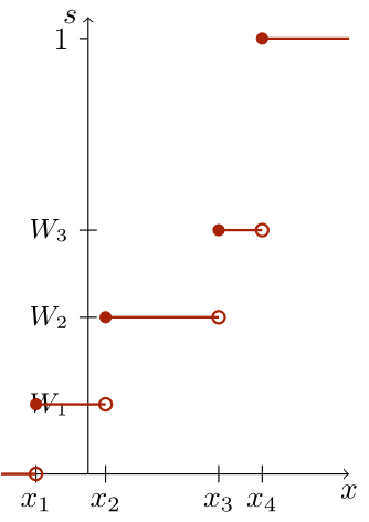
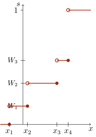
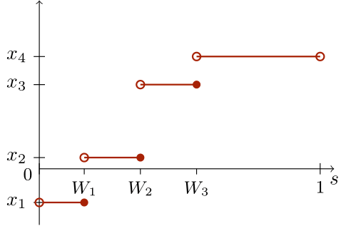
Figure 2: Functions $R_{\mu}^{+}$ (left), $R_{\mu}^{-}$ (middle) and $Q_{\mu}$ (right) for a discrete measure $\mu\coloneqq\sum_{k=1}^{4}w_{k}\delta_{x_{k}}$ with $W_{k}\coloneqq\sum_{j=1}^{k}w_{j}$. Source: [11].

Remark 2.2 (Properties of $R_{\mu}^{\pm}$ and $Q_{\mu}$).

The functions $R_{\mu}^{\pm}$ and $Q_{\mu}$ are monotonically increasing with only countably many discontinuities. The function $Q_{\mu}$ is strictly increasing if and only if $R_{\mu}^{+}$ is continuous, and continuous if and only if $R_{\mu}^{+}$ is strictly increasing on $\overline{(R_{\mu}^{+})^{-1}(0,1)}$. The points of continuity $x\in\operatorname{\mathbb{R}}$ of $R_{\mu}^{+}$ and $R_{\mu}^{-}$ coincide and there, it holds $R_{\mu}^{-}(x)=R_{\mu}^{+}(x)$. We have $R_{\mu}^{-}\leq R_{\mu}^{+}$ such that

$$[R_{\mu}^{-}(x),R_{\mu}^{+}(x)]\neq\emptyset\hskip 11.38109pt\text{ for all }x\in\operatorname{\mathbb{R}}.$$

Both $R_{\mu}^{-}$ and $Q_{\mu}$ are left-continuous and, since they are increasing, also lsc, whereas $R_{\mu}^{+}$ is right-continuous and, since it is increasing, upper semicontinuous. If $\mu(\{x\})=0$ for all $x\in\operatorname{\mathbb{R}}$, then the functions $R_{\mu}^{\pm}$ are continuous and they coincide.

The quantile functions of measures in $\mathcal{P}_{2}(\operatorname{\mathbb{R}})$ form a closed, convex cone

$$\mathcal{C}(0,1):=\{u\in L_{2}(0,1):u~{}\text{is increasing (a.e.)}\}.$$

By the following theorem, see, e.g., [21, Thm. 2.18], the mapping

$$\mathcal{I}\colon\mu\mapsto Q_{\mu}$$

is an isometric embedding of $\operatorname{\mathcal{P}}_{2}(\operatorname{\mathbb{R}})$ into $L_{2}(0,1)$.

Theorem 2.3.

For $\mu,\nu\in\operatorname{\mathcal{P}}_{2}(\operatorname{\mathbb{R}})$, the quantile function $Q_{\mu}\in\mathcal{C}(0,1)$ satisfies $\mu=(Q_{\mu})_{\#}\Lambda_{(0,1)}\coloneqq\Lambda_{(0,1)}\circ Q_{\mu}^{-1}$ with the Lebesgue measure $\Lambda_{(0,1)}$ on $(0,1)$, and $\mathcal{I}$ is an isometry, i.e.,

$$W_{2}^{2}(\mu,\nu)=\int_{0}^{1}|Q_{\mu}(s)-Q_{\nu}(s)|^{2}\mathop{}\!\mathrm{d}s.$$ (7)

The theorem gives rise to the following definition. We call a functional $F\colon L_{2}(0,1)\to(-\infty,\infty]$ associated with a functional $\operatorname{\mathcal{F}}\colon\operatorname{\mathcal{P}}_{2}(\operatorname{\mathbb{R}})\to(-\infty,\infty]$ if

$$F(Q_{\mu})=\operatorname{\mathcal{F}}(\mu)\quad\text{for all }\mu\in\operatorname{\mathcal{P}}_{2}(\operatorname{\mathbb{R}}).$$ (8)

Clearly, there are many functions $F\colon L_{2}(0,1)\to(-\infty,\infty]$ associated to a function $\operatorname{\mathcal{F}}$, since (8) determines $F$ only on $\mathcal{C}(0,1)\subset L_{2}(0,1)$. Recall that $F$ is called proper if $\operatorname{dom}(F)\coloneqq\{u\in L_{2}(0,1):F(u)<\infty\}\neq\emptyset$. Further, the regular subdifferential of a function $F\colon L_{2}(0,1)\to(-\infty,\infty]$ is defined by

$$\partial F(u)\coloneqq\bigl{\{}v\in L_{2}(0,1):F(w)\geq F(u)+\langle v,w-u\rangle+o(\|w-u\|)\;~{}\text{for all }w\in L_{2}(0,1)\bigr{\}}.$$ (9)

If $F$ is convex, the $o$-term in (9) can be skipped. If $F$ is proper, then it holds

$$\operatorname{dom}(\partial F)\coloneqq\{u\in L_{2}(0,1):\partial F(u)\neq\emptyset\}\subseteq\operatorname{dom}(F),$$

and if $F$ is in addition convex and lsc, we have $\overline{\operatorname{dom}(\partial F)}=\operatorname{dom}(F)$.

Wasserstein gradient flows can be characterized by the strong solution of a corresponding Cauchy problem in $L_{2}(0,1)$. To this end, recall that for an operator $A\colon\operatorname{dom}(A)\subseteq L_{2}(0,1)\to 2^{L_{2}(0,1)}$ and an initial function $g_{0}\in L_{2}(0,1)$, a strong solution $g\colon[0,T)\to L_{2}(0,1)$ of the Cauchy problem

$$\begin{cases}\partial_{t}g(t)+Ag(t)~{}\ni~{}0,\quad 0<t<T\leq\infty,\\ g(0)~{}=~{}g_{0},\end{cases}$$ (10)

is a locally absolutely continuous function $g\in H^{1}_{{\rm loc}}\big{(}(0,T);L_{2}(0,1)\big{)}$ which is continuous in $t=0$, meets the initial condition and solves the differential inclusion in (10) pointwise for a.e. $0<t<T$.

Theorem 2.4.

Let $\operatorname{\mathcal{F}}\colon\operatorname{\mathcal{P}}_{2}(\operatorname{\mathbb{R}})\to(-\infty,\infty]$ and let $F\colon L_{2}(0,1)\to(-\infty,\infty]$ be its associated functional as in (8). Let $g_{0}\in\mathcal{C}(0,1)$ be an initial datum. Assume, there exists a strong solution $g\colon[0,\infty)\to\mathcal{C}(0,1)$ of the Cauchy problem

$$\begin{cases}\partial_{t}g(t)+\partial F(g(t))~{}\ni~{}0,\quad t\in(0,\infty),\\ g(0)~{}=~{}g_{0}.\end{cases}$$ (11)

Then, there exists a Wasserstein gradient flow $\gamma_{t}$ of $\operatorname{\mathcal{F}}$, and it is given by $\gamma_{t}=(g(t))_{\#}\Lambda_{(0,1)}$ and $\gamma(0+)=(g_{0})_{\#}\Lambda_{(0,1)}$. Furthermore, the curve $\gamma_{t}$ has quantile functions $Q_{\gamma_{t}}=g(t)$.

With minor adjustments, the proof can be taken from [11, Theorem 3.5, part 2]. For completeness, we provide it in the appendix.

3 Distance Kernel MMDs with Sobolev Regularization

In this section, we introduce the MMD functionals for the negative as well as the positive distance kernel and their Sobolev regularized versions $\widetilde{F}_{\nu}^{-},\widetilde{F}_{\nu}^{+}$. Then, we consider flows of the negative kernel. We state the general existence of the Wasserstein gradient flow via minimizing movements, and derive a more explicit gradient flow equation (53). With it, we can give an explicit example of the $\widetilde{F}_{\nu}^{-}$-flow, and study the convergence of the gradient flow for vanishing regularization constants $\lambda\downarrow 0$. Finally, we show that there exists a so-called generalized minimizing movement in case of the positive kernel, and present an example of an $\widetilde{F}_{\nu}^{+}$-flow.

3.1 General modeling for both kernels

We consider MMD functionals given by the positive and negative distance kernel

$$K(x,y)\coloneqq\pm|x-y|,\quad x,y\in\operatorname{\mathbb{R}}.$$ (12)

The MMD between $\mu,\nu\in\mathcal{P}_{2}(\operatorname{\mathbb{R}})$ is defined by

$$\text{MMD}_{K}^{2}(\mu,\nu) \coloneqq\frac{1}{2}\int_{\operatorname{\mathbb{R}}^{2}}K(x,y)\mathop{}\!\mathrm{d}\left(\mu(x)-\nu(x)\right)\mathop{}\!\mathrm{d}\left(\mu(y)-\nu(x)\right).$$ (13)

For the negative distance kernel, the square root of the above formula defines a distance on $\operatorname{\mathcal{P}}_{2}(\operatorname{\mathbb{R}})$, so that $\text{MMD}_{K}(\mu,\nu)\geq 0$ with equality if and only if $\mu=\nu$. Fixing the target measure $\nu$ and skipping the arising constant term in (13), the MMD functionals $\operatorname{\mathcal{F}}_{\nu}^{\pm}\colon\mathcal{P}_{2}(\operatorname{\mathbb{R}})\to(-\infty,+\infty]$ are defined accordingly to the distance kernels (12) by

$$\operatorname{\mathcal{F}}_{\nu}^{\pm}(\mu)\coloneqq\frac{1}{2}\int_{\operatorname{\mathbb{R}}^{2}}\pm|x-y|\mathop{}\!\mathrm{d}\mu(x)\mathop{}\!\mathrm{d}\mu(y)-\int_{\operatorname{\mathbb{R}}^{2}}\pm|x-y|\mathop{}\!\mathrm{d}\mu(x)\mathop{}\!\mathrm{d}\nu(y).$$ (14)

The first summand is known as interaction energy, while the second one is called potential energy of $V_{\nu}\coloneqq\int_{\operatorname{\mathbb{R}}}K(\cdot,y)\mathop{}\!\mathrm{d}\nu(y)$. Functionals of this kind were, e.g., applied in [20] for function dithering. The next result from [11, 13] determines special associated functionals for $\operatorname{\mathcal{F}}_{\nu}^{\pm}(\mu)$ with convenient properties.

Lemma 3.1.

Let $\operatorname{\mathcal{F}}_{\nu}^{\pm}$ be given by (14), and let $F_{\nu}\colon L_{2}(0,1)\to\operatorname{\mathbb{R}}$ be defined by

$$F_{\nu}(u) \coloneqq\int_{0}^{1}\left((1-2s)\big{(}u(s)-Q_{\nu}(s)\big{)}+\int_{0}^{1}|u(s)-Q_{\nu}(t)|\mathop{}\!\mathrm{d}{t}\right)\mathop{}\!\mathrm{d}{s}.$$ (15)

Then, it holds for all $u\in L_{2}(0,1)$ that

$$\partial F_{\nu}(u)=\big{\{}f\in L_{2}(0,1):f(s)\in 2\big{[}R_{\nu}^{-}\big{(}u(s)\big{)},R_{\nu}^{+}\big{(}u(s)\big{)}\big{]}-2s~{}\text{for a.e.}\;s\in(0,1)\big{\}}.$$ (16)

For all $\mu\in\operatorname{\mathcal{P}}_{2}(\operatorname{\mathbb{R}})$, we have the association

$$\operatorname{\mathcal{F}}_{\nu}^{\pm}(\mu)=\mp F_{\nu}(Q_{\mu})\eqqcolon F_{\nu}^{\pm}(Q_{\mu}).$$ (17)

The functional $F_{\nu}^{-}=F_{\nu}$ corresponding to the negative kernel is convex and continuous. In particular, we have $\operatorname{dom}(\partial F_{\nu}^{-})=\operatorname{dom}(F_{\nu}^{-})=L_{2}(0,1)$. The functional $F_{\nu}^{+}=-F_{\nu}$ is in general not $\lambda$-convex for any $\lambda\in\operatorname{\mathbb{R}}$.

Proof.

Except for the last part, the result was shown in [11]. Concerning the last part, let $\lambda\in\operatorname{\mathbb{R}}$ and consider $\nu\coloneqq\delta_{0}$, so that $Q_{\nu}\equiv 0$. Assume that $F_{\nu}^{+}$ is $\lambda$-convex. Then, we have for any $u_{0},u_{1}\in L_{2}(0,1)$ that

$$F_{\nu}^{+}\left(\frac{u_{0}+u_{1}}{2}\right)\leq\frac{F_{\nu}^{+}(u_{0})+{F}_{\nu}^{+}(u_{1})}{2}-\frac{1}{8}\lambda\|u_{0}-u_{1}\|_{L_{2}(0,1)}^{2}.$$

Since the first summand of $F_{\nu}^{+}$ is linear due to $Q_{\nu}\equiv 0$, this implies

$$\int_{0}^{1}\left|u_{0}+u_{1}\right|\mathop{}\!\mathrm{d}{s} \geq\int_{0}^{1}|u_{0}|\mathop{}\!\mathrm{d}{s}+\int_{0}^{1}|u_{1}|\mathop{}\!\mathrm{d}{s}+\frac{1}{4}\lambda\int_{0}^{1}|u_{0}-u_{1}|^{2}\mathop{}\!\mathrm{d}{s}.$$

For $\varepsilon>0$ and $u_{0}\equiv\varepsilon$, $u_{1}\equiv-\varepsilon$ this implies $0\geq 2+\lambda\varepsilon$, which is a contradiction for $\varepsilon$ sufficiently small. ∎

In order to compensate for the missing convexity of $F_{\nu}^{+}$, we propose to regularize with the function $F_{H}\colon L_{2}(0,1)\to[0,\infty]$ given by

$$F_{H}(u)\coloneqq\begin{cases}\frac{\lambda}{2}\int_{0}^{1}|u^{\prime}(s)|^{2}\mathop{}\!\mathrm{d}s,&\text{if }u\in H^{1}(0,1),\\ \infty,&\text{else},\end{cases}$$ (18)

with the (diffusion) constant $\lambda>0$. The domain $\operatorname{dom}(F_{H})=H^{1}(0,1)\subset L_{2}(0,1)$ is the Sobolev space of square integrable functions $u$, whose weak first derivative $u^{\prime}$ is also square integrable. The following lemma is a classical result of the PDE theory and can be found, e.g., in [4, Proposition 2.9].

Lemma 3.2.

The functional $F_{H}$ in (18) is proper, convex and lsc. The subdifferential $\partial F_{H}(u)$ of $F_{H}$ at $u\in L_{2}(0,1)$ consists of all $f\in L_{2}(0,1)$ such that $u$ is the weak solution of the problem

$$\lambda\int_{0}^{1}u^{\prime}(s)v^{\prime}(s)\mathop{}\!\mathrm{d}s=\int_{0}^{1}f(s)v(s)\mathop{}\!\mathrm{d}s\quad\text{for all }v\in H^{1}(0,1).$$ (19)

Further, $\operatorname{dom}(\partial F_{H})$ is dense in $L_{2}(0,1)$ and is given by

$$\operatorname{dom}(\partial F_{H}) =\{u\in H^{1}(0,1):u^{\prime\prime}\in L_{2}(0,1)\text{ and }\,u^{\prime}(0)=u^{\prime}(1)=0\}$$ (20)

$$=\{u\in H^{2}(0,1):u^{\prime}(0)=u^{\prime}(1)=0\}$$ (21)

where $u^{\prime\prime}$ denotes the second weak derivative of $u$. For $u\in\operatorname{dom}(\partial F_{H})$, it holds $\partial F_{H}(u)=-\lambda u^{\prime\prime}$.

Regularizing $F_{\nu}^{-}$ directly with the functional $F_{H}$ leads to a distortion of the target $\nu$. Therefore, we consider for $Q_{\nu}\in H^{1}(0,1)$ the function $F_{H,\nu}\colon L_{2}(0,1)\to[0,\infty]$ with

$$F_{H,\nu}(u)\coloneqq F_{H}(u-Q_{\nu}).$$ (22)

It is also proper, convex, lsc and $\operatorname{dom}(F_{H,\nu})=\operatorname{dom}(F_{H})=H^{1}(0,1)$. Further, it holds $\partial F_{H,\nu}(u)=\partial F_{H}(u-Q_{\nu})$ for all $u\in H^{1}(0,1)$ and $\operatorname{dom}(\partial F_{H,\nu})=\operatorname{dom}(\partial F_{H})+Q_{\nu}$. If $Q_{\nu}\in H^{2}(0,1)$, then we have

$$\operatorname{dom}(\partial F_{H,\nu})=\{u\in H^{2}(0,1):u^{\prime}(0)=Q_{\nu}^{\prime}(0),~{}u^{\prime}(1)=Q_{\nu}^{\prime}(1)\}$$

and

$$\partial F_{H,\nu}(u)=-\lambda u^{\prime\prime}+\lambda Q_{\nu}^{\prime\prime}\qquad\text{for all }u\in\operatorname{dom}(\partial F_{H,\nu}).$$

To ensure that the gradient flow stays in $\operatorname{\mathcal{C}}(0,1)$, we use the indicator function

$$I_{\operatorname{\mathcal{C}}(0,1)}(u)\coloneqq\begin{cases}0,\quad~{}\,\text{if }u\in\operatorname{\mathcal{C}}(0,1),\\ \infty,\quad\text{else},\end{cases}$$ (23)

which is proper, convex and lsc, since $\operatorname{\mathcal{C}}(0,1)$ is nonempty, convex and closed. Further, $\operatorname{dom}(\partial I_{\operatorname{\mathcal{C}}(0,1)})=\operatorname{\mathcal{C}}(0,1)$, and it holds $0\in\partial I_{\operatorname{\mathcal{C}}(0,1)}(u)$ for all $u\in\operatorname{\mathcal{C}}(0,1)$. Now, we can introduce the regularized versions $\widetilde{F}_{\nu}^{\pm}\colon L_{2}(0,1)\to(-\infty,\infty]$ of $F_{\nu}^{\pm}$ given by

$$\widetilde{F}_{\nu}^{-} \coloneqq F_{\nu}^{-}+F_{H,\nu}+I_{\operatorname{\mathcal{C}}(0,1)},\qquad\widetilde{F}_{\nu}^{+}\coloneqq F_{\nu}^{+}+F_{H}+I_{\operatorname{\mathcal{C}}(0,1)}.$$ (24)

It holds that $\operatorname{dom}(\widetilde{F}_{\nu}^{\pm})=\operatorname{\mathcal{C}}(0,1)\cap H^{1}(0,1)$.

Remark 3.3 ($\widetilde{F}_{\nu}^{\pm}$ as associated functions of $\widetilde{\mathcal{F}}_{\nu}^{\pm}$).

Using Lemma 3.1 and the isometry $\mathcal{I}$ from Theorem 2.3, we see that $\widetilde{F}_{\nu}^{\pm}\colon L_{2}(0,1)\to(-\infty,\infty]$ are associated functionals of $\widetilde{\operatorname{\mathcal{F}}}_{\nu}^{\pm}\colon\mathcal{P}_{2}(\operatorname{\mathbb{R}})\to(-\infty,\infty]$ given by

$$\widetilde{\operatorname{\mathcal{F}}}_{\nu}^{-}(\mu)\coloneqq\operatorname{\mathcal{F}}_{\nu}^{-}(\mu)+F_{H,\nu}(\mathcal{I}(\mu))\quad\text{and}\quad\widetilde{\operatorname{\mathcal{F}}}_{\nu}^{+}(\mu)\coloneqq\operatorname{\mathcal{F}}_{\nu}^{+}(\mu)+F_{H}(\mathcal{I}(\mu)).$$ (25)

If $\mu\in\operatorname{\mathcal{P}}_{2}(\operatorname{\mathbb{R}})$ has a density $f_{\mu}\in L^{1}(\operatorname{\mathbb{R}})$, then the squared $H^{1}$-seminorm of $Q_{\mu}$ becomes

$$|Q_{\mu}|_{1,2}^{2} =\int_{\operatorname{supp}(\mu)}\frac{1}{f_{\mu}(x)}\mathop{}\!\mathrm{d}{x},$$

which delivers the second summand in the above functionals. Note that this expression would also make sense in higher dimensions which we will consider in our future work.

3.2 Flows of the negative kernel

We consider the function $\widetilde{F}_{\nu}^{-}$. Let us start with the existence result.

Theorem 3.4.

For $Q_{\nu}\in\operatorname{\mathcal{C}}(0,1)\cap H^{1}(0,1)$, let $\widetilde{F}_{\nu}^{-}$ be given by (24), and suppose an initial datum $g_{0}\in\operatorname{dom}(\widetilde{F}_{\nu}^{-})=\operatorname{\mathcal{C}}(0,1)\cap H^{1}(0,1)$. Then, there exists a unique strong solution $g\in H^{1}_{\rm loc}([0,\infty);L_{2}(0,1))$ of the Cauchy problem

$$\begin{cases}\partial_{t}g(t)\in-\partial\widetilde{F}_{\nu}^{-}(g(t)),\quad t\in(0,\infty),\\ g(0)=g_{0}.\end{cases}$$ (26)

The associated curve $\gamma_{t}\coloneqq(g(t))_{\#}\Lambda_{(0,1)}$ is the unique Wasserstein gradient flow of $\widetilde{\operatorname{\mathcal{F}}}_{\nu}^{-}$ on $(0,\infty)$ with $\gamma(0+)=(g_{0})_{\#}\Lambda_{(0,1)}$. Both flows $g$ and $\gamma_{t}$ are given by minimizing movements $g\in{\rm MM}(\widetilde{F}_{\nu}^{-},g_{0})$ and $\gamma\in{\rm MM}(\widetilde{\operatorname{\mathcal{F}}}_{\nu}^{-},\gamma(0+))$, respectively. The minimizers (5) are unique and the convergence (6) is uniform in the stepsize $\tau$.

Proof.

Since $\widetilde{F}_{\nu}^{-}$ and $\widetilde{\operatorname{\mathcal{F}}}_{\nu}^{-}$ are proper, convex and lsc, the result follows from combining Remark 3.3, Theorem 2.4 and the standard literature of maximal monotone/subdifferential operators, see, e.g., [8], and also [1] for the Wasserstein setting. ∎

Remark 3.5 (Purpose of the $F_{H,\nu}$-regularization).

To be clear, the functional $F_{\nu}^{-}=F_{\nu}$ associated with the negative kernel is already convex (in one dimension), and technically, the existence of strong solutions $g\in{\rm MM}({F}_{\nu}^{-},g_{0})$ is already known. Nevertheless, the regularization via $F_{H,\nu}$ rectifies a "dissipation-of-mass defect" of the $F_{\nu}$-flow as demonstrated in Section 4.2. This might be useful when working on $\operatorname{\mathcal{P}}_{2}(\operatorname{\mathbb{R}}^{d})$ since there, the non-convexity of the negative kernel MMD paired with this defect seems to complicate the proof of the existence of Wasserstein gradient flows.

By the following proposition, under mild assumptions on the target, the indicator function $I_{\operatorname{\mathcal{C}}(0,1)}$ is actually not needed when considering the gradient flow of $\widetilde{F}_{\nu}^{-}$. These assumptions are fulfilled, e.g., if $Q_{\nu}\in C^{3}([0,1])$ and $\lambda>0$ is sufficiently small; or more generally, if $Q_{\nu}\in H^{3}(0,1)$ and

$$Q_{\nu}^{\prime\prime\prime}(s)\leq\frac{2}{\lambda}\quad\text{for all }s\in(0,1).$$ (27)

Together with Lemma 3.1 and 3.2, we obtain an explicit form of the gradient flow equation (26).

Proposition 3.6.

Assume that $Q_{\nu}\in H^{2}(0,1)$ and $\lambda>0$ such that the function

$$(0,1)\to\operatorname{\mathbb{R}},~{}~{}s\mapsto 2s-\lambda Q_{\nu}^{\prime\prime}(s)\quad\text{is non-decreasing (except for nullset)}.$$ (28)

Then, for any $g_{0}\in H^{1}(0,1)\cap\operatorname{\mathcal{C}}(0,1)$, the unique strong solution of the Cauchy problem

$$\begin{cases}\partial_{t}g(t)+\partial F_{\nu}(g(t))+\partial F_{H,\nu}(g(t))\ni 0,\quad t\in(0,\infty),\\ g(0)=g_{0},\end{cases}$$ (29)

exists, and it coincides with the unique strong solution $g$ of (26). In particular, it satisfies the invariance property $g(t)\in\operatorname{\mathcal{C}}(0,1)$ for all $t\geq 0$.

Proof.

Note that by [17, Theorem 3.16], it holds the equality $\partial F_{\nu}+\partial F_{H,\nu}=\partial(F_{\nu}+F_{H,\nu})$, since the Rockafellar interior condition

$${\rm int}\big{(}\operatorname{dom}(F_{\nu})\big{)}\cap\operatorname{dom}(F_{H,\nu})=L_{2}(0,1)\cap H^{1}(0,1)\neq\emptyset$$ (30)

is fulfilled by Lemma 3.1. Now, $F_{\nu}+F_{H,\nu}$ is proper, convex and lsc with $\operatorname{dom}(F_{\nu}+F_{H,\nu})=H^{1}(0,1)$. Then, by standard results about subdifferential operators, see [8, Theorem 3.6], there exists a unique strong solution $g$ of (29).

To show that $g$ also solves (26), we only need to prove that $g(t)\in\operatorname{\mathcal{C}}(0,1)$ for all $t\geq 0$, since this implies

$$\partial F_{\nu}(g(t))+\partial F_{H,\nu}(g(t))+\{0\} \subseteq\partial F_{\nu}(g(t))+\partial F_{H,\nu}(g(t))+\partial I_{\operatorname{\mathcal{C}}(0,1)}(g(t))$$ (31)

$$\subseteq\partial(F_{\nu}+F_{H,\nu}+I_{\operatorname{\mathcal{C}}(0,1)})(g(t))=\partial\widetilde{F}_{\nu}^{-}(g(t)).$$ (32)

To this end, let $\tau>0$ and consider the implicit Euler scheme with stepsize $\tau>0$ of (29) given by

$$g_{n+1}(s)+2\tau[R_{\nu}^{-}(g_{n+1}(s)),R_{\nu}^{+}(g_{n+1}(s))]-2\tau s-\tau\lambda g_{n+1}^{\prime\prime}(s)+\tau\lambda Q_{\nu}^{\prime\prime}(s)\ni g_{n}(s)\quad\text{for a.e. }s\in(0,1),$$ (33)

where the existence of $g_{n+1}\in\operatorname{dom}(\partial F_{H,\nu})$ is obtained via the maximal monotonicity of $\partial F_{H,\nu}+\partial F_{\nu}$. We need to show that $g_{n}\in\operatorname{\mathcal{C}}(0,1)$ implies $g_{n+1}\in\operatorname{\mathcal{C}}(0,1)$. Then, the assertion follows by the arguments in [11, Corollary 3.6].

So let $g_{n}\in\operatorname{\mathcal{C}}(0,1)$, and assume that there exists $s_{0}\in(0,1)$ such that $g_{n+1}^{\prime}(s_{0})<0$. Note that by assumption, $Q_{\nu}\in H^{2}(0,1)$ is continuously differentiable on $[0,1]$. Since $Q_{\nu}$ is increasing, it must hold $Q_{\nu}^{\prime}(0),\,Q_{\nu}^{\prime}(1)\geq 0$. Now, since $g_{n+1}\in\operatorname{dom}(\partial F_{H,\nu})=\{u\in H^{2}(0,1):u^{\prime}(0)=Q_{\nu}^{\prime}(0),~{}u^{\prime}(1)=Q_{\nu}^{\prime}(1)\}$, we have that $g_{n+1}$ is continuously differentiable with $g_{n+1}^{\prime}(s_{0})<0\leq\min\{g_{n+1}^{\prime}(0),\,g_{n+1}^{\prime}(1)\}$. Hence, by the continuity of $g_{n+1}^{\prime}$, there exists an interval $\emptyset\neq(a,b)\subset(0,1)$ around $s_{0}$ such that $g_{n+1}^{\prime}(s)<0$ for all $s\in(a,b)$, and $g_{n+1}^{\prime}(a)=g_{n+1}^{\prime}(b)=0$. In particular, $g_{n+1}$ is strictly decreasing on $(a,b)$. Now, it holds

$$-\tau\lambda g_{n+1}^{\prime\prime}(s)\in g_{n}(s)-g_{n+1}(s)+2\tau[-R_{\nu}^{+}(g_{n+1}(s)),-R_{\nu}^{-}(g_{n+1}(s))]+\tau(2s-\lambda Q_{\nu}^{\prime\prime}(s))$$ (34)

for a.e. $s\in(a,b)$. Since $g_{n}$ is increasing, $g_{n+1}$ is strictly decreasing and by assumption (28), we have for a.e. $s_{1},s_{2}\in(a,b)$ with $s_{1}<s_{2}$ that

$$-\tau\lambda g_{n+1}^{\prime\prime}(s_{1}) \leq g_{n}(s_{1})-g_{n+1}(s_{1})-2\tau R_{\nu}^{-}(g_{n+1}(s_{1}))+\tau(2s_{1}-\lambda Q_{\nu}^{\prime\prime}(s_{1}))$$ (35)

$$<g_{n}(s_{2})-g_{n+1}(s_{2})-2\tau R_{\nu}^{+}(g_{n+1}(s_{2}))+\tau(2s_{2}-\lambda Q_{\nu}^{\prime\prime}(s_{2}))$$ (36)

$$\leq-\tau\lambda g_{n+1}^{\prime\prime}(s_{2}).$$ (37)

This means that, outside a nullset, $-g_{n+1}^{\prime\prime}$ is increasing on $(a,b)$, or $g_{n+1}^{\prime\prime}$ is decreasing on $(a,b)$. Finally, note that $g_{n+1}^{\prime}(a)=0>g_{n+1}^{\prime}(s_{0})$, and by the absolute continuity of $g_{n+1}^{\prime}$, there must exist $A_{1}\subseteq(a,s_{0})$ with positive Lebesgue measure such that $g_{n+1}^{\prime\prime}(\xi_{1})<0$ for all $\xi_{1}\in A_{1}$. At the same time, since $g_{n+1}^{\prime}(s_{0})<0=g_{n+1}^{\prime}(b)$, there must exist $A_{2}\subseteq(s_{0},b)$ with positive mass such that $g_{n+1}^{\prime\prime}(\xi_{2})>0$ for all $\xi_{2}\in A_{2}$. Hence, $g_{n+1}^{\prime\prime}(\xi_{1})<0<g_{n+1}^{\prime\prime}(\xi_{2})$ for all $\xi_{1}\in A_{1},\,\xi_{2}\in A_{2}$, but $g_{n+1}^{\prime\prime}$ is decreasing on $(a,b)$ outside a nullset.

This contradiction implies $g_{n+1}^{\prime}(s)\geq 0$ for all $s\in(0,1)$, from which we infer that $g_{n+1}$ is increasing on $(0,1)$, i.e., $g_{n+1}\in\operatorname{\mathcal{C}}(0,1)$, and we are done. ∎

With Proposition 3.6, we can study the $\widetilde{F}_{\nu}^{-}$-gradient flow between two Dirac measures.

Example 3.7 (Flow of $\widetilde{F}_{\nu}^{-}$ from $\delta_{-1}$ to $\delta_{0}$).

We consider as target the Dirac measure $\nu\coloneqq\delta_{0}$, and as initial measure $\gamma_{0}\coloneqq\delta_{-1}$. The corresponding quantiles are $Q_{\nu}\equiv 0$ and $g_{0}\equiv-1$. Let $g(t,s)\coloneqq\left(g(t)\right)(s)$. Then, by Proposition 3.6 and Lemma 3.1, for any $\lambda>0$ the $\widetilde{F}_{\nu}^{-}$-flow is given by the differential inclusion

$$\partial_{t}g(t,s)+\partial F_{H,\nu}(g(t))(s)\in 2s-2H(g(t,s)),\quad\text{for a.e. }t\in(0,\infty),\,\text{a.e. }s\in(0,1),$$ (38)

with the set-valued Heaviside function

$$H(x)\coloneqq\begin{cases}0,&x<0,\\ 1,&x>0,\\ [0,1],&x=0.\end{cases}$$

Hence, for all $0<t<t^{*}$, where $t^{*}>0$ is the first point in time when $g(t^{*},\cdot)$ touches the constant $Q_{\nu}\equiv 0$, the inclusion (38) becomes the heat equation with homogeneous Neumann boundary conditions and inhomogeneity $2s$, i.e.,

$${\rm(HEAT)}\begin{cases}&\partial_{t}g(t,s)-\lambda\partial^{2}_{ss}g(t,s)=2s,\quad t\in(0,t^{*}),~{}s\in(0,1),\\ &\partial_{s}g(t,0)=\partial_{s}g(t,1)=0,\qquad t\in(0,t^{*}),\\ &g(0,\cdot)\equiv-1.\end{cases}$$ (39)

Using Fourier series, the solution to (39) can be explicitly computed: inserting the Ansatz

$$u(t,s)=\frac{c_{0}(t)}{2}+\sum_{n=1}^{\infty}c_{n}(t)\cos(n\pi s)$$ (40)

into (39) yields

$$\frac{c_{0}^{\prime}(t)}{2}+\sum_{n=1}^{\infty}[c_{n}^{\prime}(t)+\lambda(n\pi)^{2}c_{n}(t)]\cos(n\pi s)=2s\eqqcolon\frac{b_{0}}{2}+\sum_{n=1}^{\infty}b_{n}\cos(n\pi s),$$ (41)

where the right-hand side defines the Fourier series of $f(s)=2s$ evenly extended to $(-1,1)$. Hence,

$$c_{0}^{\prime}(t)=b_{0}:=2\int_{0}^{1}f(s)\mathop{}\!\mathrm{d}s=2,$$ (42)

and for $n\geq 1$, we obtain

$$c_{n}^{\prime}(t)+\lambda(n\pi)^{2}c_{n}(t)=b_{n}:=2\int_{0}^{1}f(s)\cos(n\pi s)\mathop{}\!\mathrm{d}s=\frac{4(\cos(n\pi)-1)}{(n\pi)^{2}}.$$ (43)

Using the initial condition $u(0,\cdot)\equiv-1$, we get

$$c_{0}(t)=2(t-1)\quad\text{and}\quad c_{n}(t)=\frac{b_{n}}{\lambda(n\pi)^{2}}(1-e^{-\lambda(n\pi)^{2}t}).$$ (44)

Altogether, the explicit solution of (39) up to the time $t<t^{*}$ reads as

$$u(t,s)=(t-1)+\frac{1}{\lambda}\sum_{n=1,n\,{\rm odd}}^{\infty}(-8)(n\pi)^{-4}(1-e^{-\lambda(n\pi)^{2}t})\cos(n\pi s),\quad t\in(0,t^{*}),\,s\in(0,1).$$ (45)

For $t\geq t^{*}$, the solution is given by the following free boundary problem, or Stefan problem,

$${\rm(STEFAN)}\begin{cases}&\partial_{t}g(t,s)-\lambda\partial^{2}_{ss}g(t,s)=2s,\quad t\in(t^{*},\infty),\,s\in(0,\beta(t)),\\ &\partial_{s}g(t,0)=\partial_{s}g(t,\beta(t))=0,\quad t\in(t^{*},\infty),\\ &g(t,s)=0,\quad s\in[\beta(t),1),~{}t\in(t^{*},\infty),\\ &g(t^{*},\cdot)=u(t^{*},\cdot),\end{cases}$$ (46)

where the right moving boundary function $\beta\colon[t^{*},\infty)\to(0,1]$ with $\beta(t^{*})=1$ is part of the solution $(g,\beta)$. Since this problem is more involved, and no explicit representation via Fourier series can be expected, we will approximate the solution in the numerical Section 4.2. $\Box$

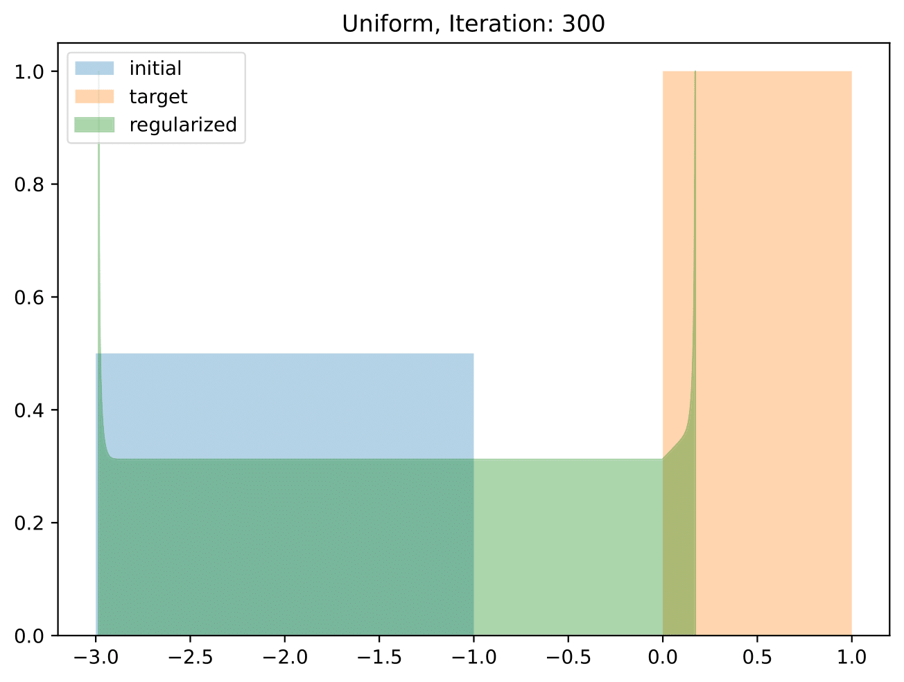
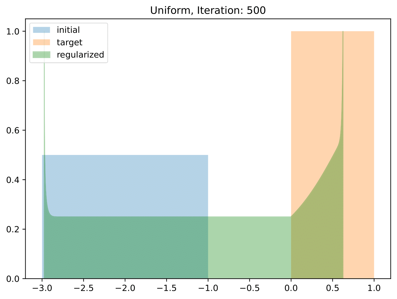
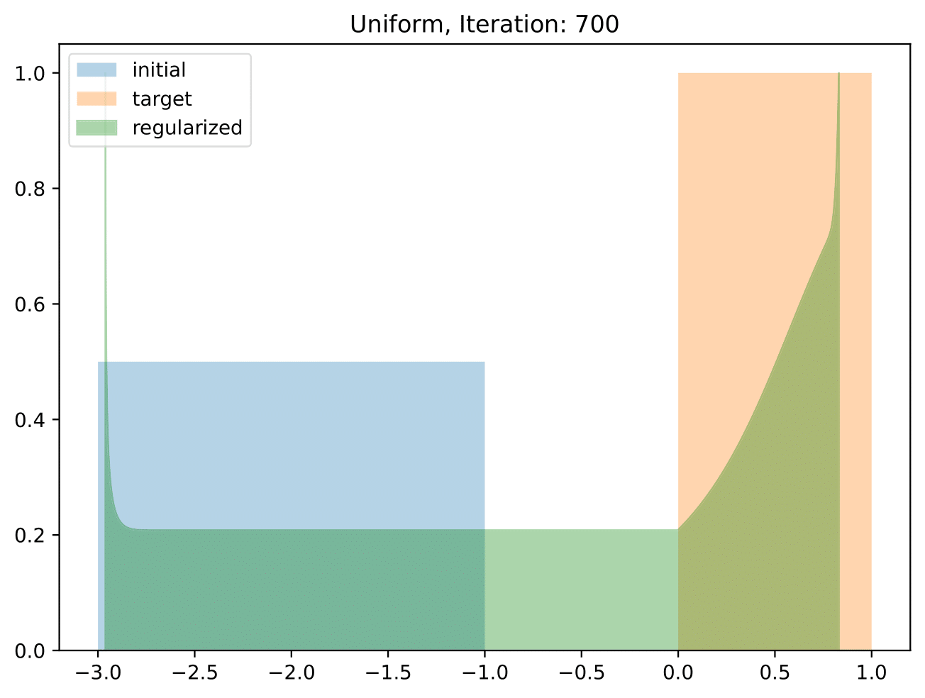
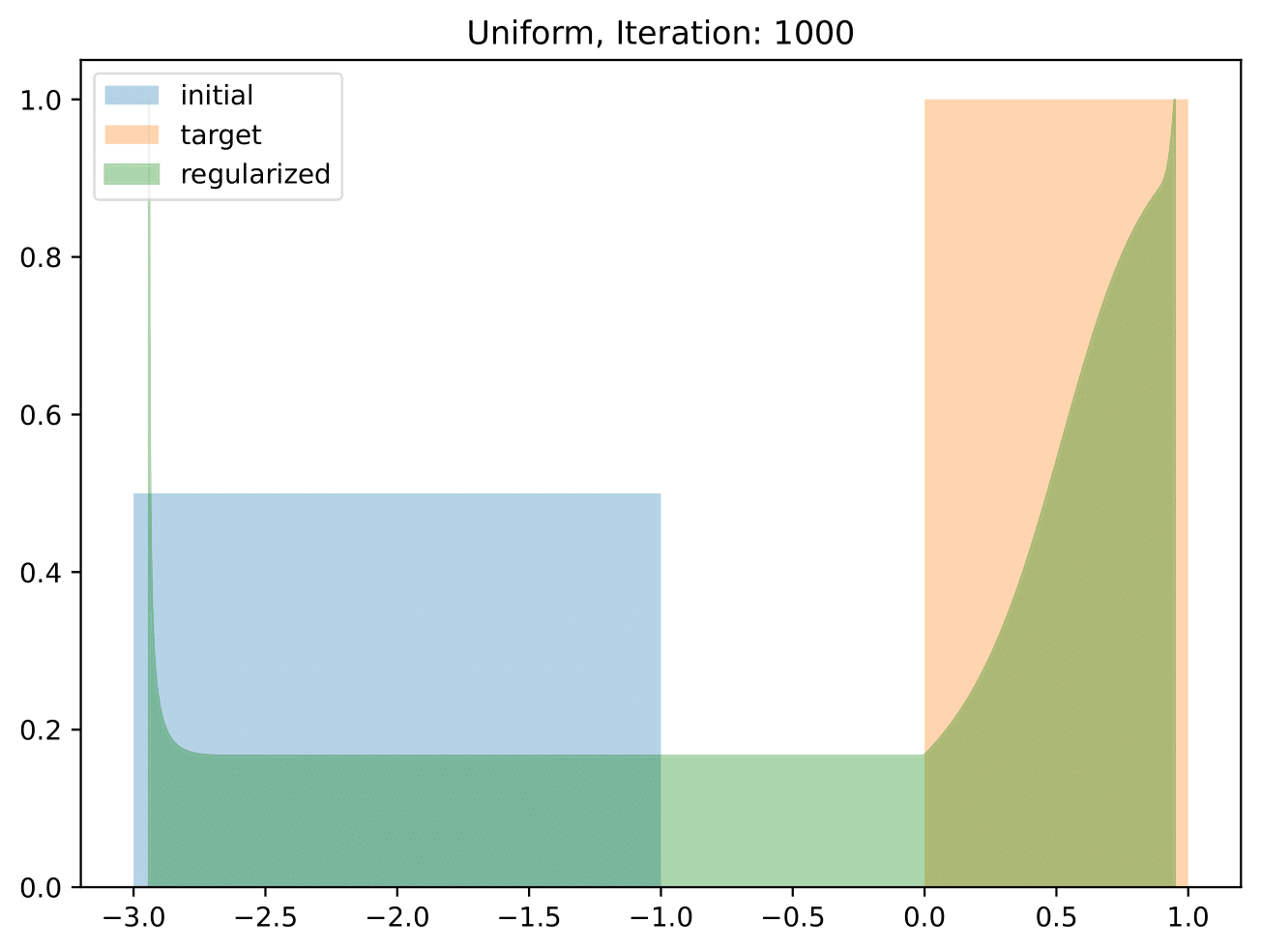
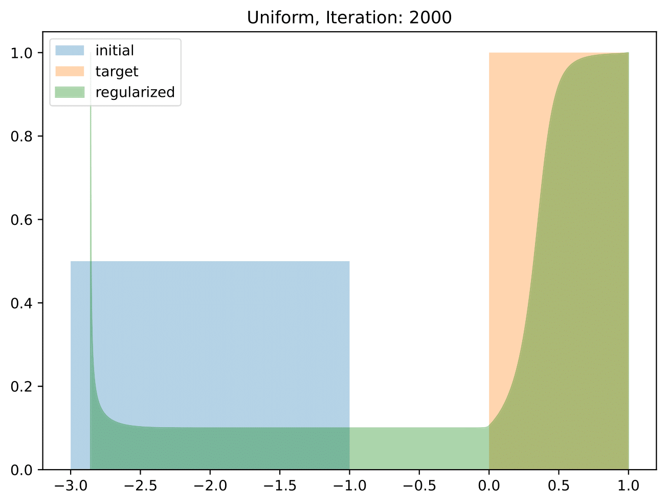
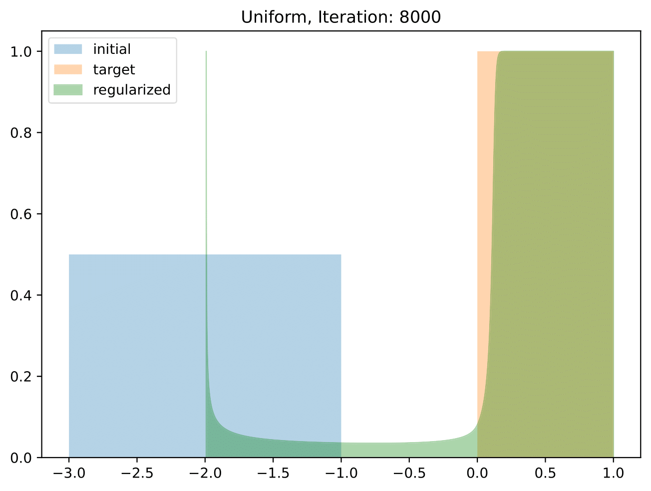
Figure 13: Regularized ${\mathcal{F}}_{\nu}^{-}$-flow between the uniform measures $\gamma_{0}\sim\mathcal{U}[-3,-1]$ and $\nu\sim\mathcal{U}[0,1]$ for $\tau=2\cdot 10^{-3}$ and "small" $\lambda=10^{-4}$. The support shifts only slowly towards the target but expands quickly, similar to the unregularized flow for small times.

Let us quickly examine the behavior of the flow (29) of the negative kernel for vanishing diffusion constants $\lambda$, see also the Figure 13 in the appendix.

Remark 3.8 (Convergence for $\lambda\downarrow 0$).

Let us explicitly denote the dependence on the diffusion constant $\lambda>0$ by ${F}_{\nu}^{\lambda}=F_{H,\nu}^{\lambda}+F_{\nu}$, where again, the functional $F_{H,\nu}^{\lambda}\colon H^{1}(0,1)\subset L_{2}(0,1)\to[0,\infty]$ is given by

$$F_{H,\nu}^{\lambda}(w)=\begin{cases}\displaystyle\frac{\lambda}{2}\int_{0}^{1}|w^{\prime}(s)-Q_{\nu}^{\prime}(s)|^{2}\mathop{}\!\mathrm{d}s,&\text{if }w\in H^{1}(0,1),\\ \infty,&\text{else}.\end{cases}$$ (47)

Let $(\lambda_{n})$ be an arbitrary zero sequence of positive numbers, then the Mosco convergence of $F_{\nu}^{\lambda_{n}}$ to $F_{\nu}$ for $n\to\infty$ is immediate: Let $u\in L_{2}(0,1)$, then for any sequence $u_{n}\rightharpoonup u$ in $L_{2}(0,1)$, it clearly holds by the nonnegativity of $F_{H,\nu}^{\lambda_{n}}$ and weak lower semicontinuity of $F_{\nu}$ that

$$F_{\nu}(u)\leq\liminf_{n\to\infty}F_{H,\nu}^{\lambda_{n}}(u_{n})+F_{\nu}(u_{n})=\liminf_{n\to\infty}{F}_{\nu}^{\lambda_{n}}(u_{n}).$$ (48)

Lastly, since $H^{1}(0,1)$ is dense in $L_{2}(0,1)$, there exists a sequence $v_{n}\in H^{1}(0,1)$ with $v_{n}\to u$ in $L_{2}(0,1)$ such that $\lambda_{n}\,|v_{n}|_{H^{1}}\to 0$, and hence by the continuity of $F_{\nu}$,

$$F_{\nu}(u)=\lim_{n\to\infty}F_{H,\nu}^{\lambda_{n}}(v_{n})+F_{\nu}(v_{n})=\lim_{n\to\infty}{F}_{\nu}^{\lambda_{n}}(v_{n}).$$ (49)

Now, by classical convergence results of semigroup theory, see [9, 3], and also [5] for an extensive presentation, it holds the convergence

$$\lim_{n\to\infty}\sup_{t\in[0,T]}\|g_{\lambda_{n}}(t)-g(t)\|_{L_{2}(0,1)}=0,$$ (50)

where $g_{\lambda_{n}},g$ are the unique solutions of (29) with respect to diffusion constants $\lambda_{n}$ and $\lambda=0$, respectively. $\Box$

3.3 Flows of the positive kernel

Since for the positive kernel, the functional $F_{\nu}^{+}$ is in general not $\lambda$-convex due to Lemma 3.1, its treatment is more involved, and in general, the existence of a Wasserstein gradient flow cannot be expected. Yet, the proposed regularization allows for a description of the flow via the generalized minimizing movement (GMM) scheme, see also [19]:

Given $g_{0}\in L_{2}(0,1)$ and $F\colon L_{2}(0,1)\to(-\infty,\infty]$, consider piecewise constant curves $g_{\tau}$ constructed from the (possibly non-unique) minimizers

$$g_{n+1}\in\operatorname*{arg\,min}_{v\in L_{2}(0,1)}\Big{\{}F(v)+\frac{1}{2\tau}\|g_{n}-v\|_{L_{2}(0,1)}^{2}\Big{\}},\quad\tau>0,$$ (51)

via $g_{\tau}|_{(n\tau,(n+1)\tau]}\coloneqq g_{n},~{}n\in\operatorname{\mathbb{N}}_{0}$. We say that $g$ is a Generalized Minimizing Movement, if there exists a subsequence $\tau_{k}\downarrow 0$ and a corresponding family of discrete curves $(g_{\tau_{k}})$ such that

$$\lim_{k\to\infty}g_{\tau_{k}}(t)=g(t)\quad\text{for all }t\in[0,T],$$ (52)

where the limit is taken in $L_{2}(0,1)$, and we write $g\in{\rm GMM}(F,g_{0})$.

With this concept, we can describe a flow of $\widetilde{F}_{\nu}^{+}$ via generalized minimizing movements. We will make use of the results in [19]. For convenience we provide them in the appendix.

Theorem 3.9.

For $Q_{\nu}\in\operatorname{\mathcal{C}}(0,1)$, let $\widetilde{F}_{\nu}^{+}$ be given by (24). Suppose that the initial datum fulfills $g_{0}\in\operatorname{dom}(\widetilde{F}_{\nu}^{+})=\operatorname{\mathcal{C}}(0,1)\cap H^{1}(0,1)$. Then, for any $0<T<\infty$, there exist functions $g\in{\rm GMM}(\widetilde{F}_{\nu}^{+},g_{0})$, and they are strong solutions $g\in H^{1}(0,T;L_{2}(0,1))$ of the Cauchy problem

$$\begin{cases}\partial_{t}g(t)\in-\partial_{l}\widetilde{F}_{\nu}^{+}(g(t)),\quad t\in(0,T),\\ g(0)=g_{0}.\end{cases}$$ (53)

Here, $\partial_{l}\widetilde{F}_{\nu}^{+}$ denotes the limiting subdifferential, see [19]. The associated curve $\gamma_{t}\coloneqq(g(t))_{\#}\Lambda_{(0,1)}$ is a Wasserstein absolutely continuous flow on $(0,T)$ with $\gamma(0+)=(g_{0})_{\#}\Lambda_{(0,1)}$, and it is given by $\gamma\in{\rm GMM}(\widetilde{\operatorname{\mathcal{F}}}_{\nu}^{+},\gamma(0+))$.

Proof.

Note that $\widetilde{F}_{\nu}^{+}$ and $g_{0}$ satisfy the compactness criterion of [19, Lemma 1.2] by the compact Sobolev embedding $H^{1}(0,1)\overset{c}{\hookrightarrow}L_{2}(0,1)$. Furthermore, since the functionals $F_{H}+F_{\operatorname{\mathcal{C}}(0,1)}$ and $F_{\nu}$ are convex and lsc, and since $\operatorname{dom}(\partial F_{\nu})=L_{2}(0,1)$ by Lemma 3.1, the conditions of [19, Remark 1.9] are fulfilled. Therefore, [19, Theorem 3] yields the existence of a strong solution $g\in H^{1}(0,T;L_{2}(0,1))$ of (53) via generalized minimizing movements $g\in{\rm GMM}(\widetilde{F}_{\nu}^{+},g_{0})$ for any $0<T<\infty$. The remaining part follows directly by using the isometry of Theorem 2.3, and Remark 3.3. ∎

Remark 3.10 (Purpose of the $F_{H}$-regularization).

Since the associated functional $F_{\nu}^{+}=-F_{\nu}$ may lack any form of $\lambda$-convexity by Lemma 3.1, the existence of generalized minimizing movements $g\in{\rm GMM}(F_{\nu}^{+},g_{0})$ might not be given in general. Although it can be shown that the minimizers in (51) exist, the convergence (52) of the discrete solutions is unclear in general. On a technical level, regularizing via the Sobolev norm $F_{H}$ gives control over the convergence (52), ensuring that $g\in{\rm GMM}(\widetilde{F}_{\nu}^{+},g_{0})$ always exists.

As stated in Remark 3.10 the regularization via $F_{H}$ plays more of a technical role ensuring general existence of generalized minimizing movements. Nevertheless, in the following example it is not needed, and we can explicitly calculate $g\in{\rm GMM}(\widetilde{F}_{\nu}^{+},g_{0})$.

Example 3.11 (Flow of $\widetilde{F}_{\nu}^{+}$ from $\delta_{-1}$ away from $\delta_{0}$).

Let $\tau>0$ be a positive step size and $g<0$ some constant function, where we denote both the function and the constant by $g$. The minimizer (51) of one step of the GMM scheme is given by

$$\operatorname*{arg\,min}_{f\in L_{2}(0,1)} \left\{\widetilde{F}_{\nu}^{+}(f)+\frac{1}{2\tau}\int_{0}^{1}|g-f(x)|^{2}\mathop{}\!\mathrm{d}x\right\}$$ (54)

$$=\operatorname*{arg\,min}_{f\in\mathcal{C}(0,1)\cap H^{1}(0,1)} \Big{\{}-\int_{0}^{1}\left((1-2s)f(s)+|f(s)|\right)\mathop{}\!\mathrm{d}s+\frac{\lambda}{2}\int_{0}^{1}|f^{\prime}(x)|^{2}\mathop{}\!\mathrm{d}x$$ (55)

$$+ \frac{1}{2\tau}\int_{0}^{1}|g-f(x)|^{2}\mathop{}\!\mathrm{d}x\Big{\}}.$$ (56)

Next we show that the minimizer in (56) is a constant function. Let $f\in\mathcal{C}(0,1)\cap H^{1}(0,1)$ and set $\bar{f}\coloneqq-\int_{0}^{1}|f(s)|\mathop{}\!\mathrm{d}s\leq 0$. We consider the summands of (56) separately. Obviously, the Sobolev term favors the constant function $\bar{f}$, because

$$\int_{0}^{1}|\bar{f}^{\prime}|^{2}\mathop{}\!\mathrm{d}\lambda=0\leq\int_{0}^{1}|f^{\prime}|^{2}\mathop{}\!\mathrm{d}\lambda,$$

where the inequality is strict if $f$ is not constant. Further, we have for $g<0$ that

$$\int_{0}^{1}|g-\bar{f}|^{2}\mathop{}\!\mathrm{d}x =|g-\bar{f}|^{2}=\left(\int_{0}^{1}g+|f(x)|\mathop{}\!\mathrm{d}x\right)^{2}\leq\left(\int_{0}^{1}\bigl{|}g+|f(x)|\bigr{|}\mathop{}\!\mathrm{d}x\right)^{2}$$

$$=\left(\int_{0}^{1}\bigl{|}|f(x)|-|g|\bigr{|}\mathop{}\!\mathrm{d}x\right)^{2}\leq\left(\int_{0}^{1}|f(x)-g|\mathop{}\!\mathrm{d}x\right)^{2}\leq\int_{0}^{1}|g-f(x)|^{2}\mathop{}\!\mathrm{d}x.$$

Finally,

$$-\int_{0}^{1}|f(s)|\mathop{}\!\mathrm{d}s=\bar{f}=-\int_{0}^{1}|\bar{f}|\mathop{}\!\mathrm{d}s,$$

and for the remaining summand we have by monotonicity of $f$ that

$$-\int_{0}^{1}(1-2s)f(s)\mathop{}\!\mathrm{d}s =-\int_{0}^{1}(1-2s)\int_{0}^{s}f^{\prime}(t)\mathop{}\!\mathrm{d}t\mathop{}\!\mathrm{d}s=-\int_{0}^{1}f^{\prime}(t)\int_{t}^{1}(1-2s)\mathop{}\!\mathrm{d}s\mathop{}\!\mathrm{d}t$$

$$=-\int_{0}^{1}f^{\prime}(t)[s-s^{2}]_{t}^{1}\mathop{}\!\mathrm{d}t=\int_{0}^{1}f^{\prime}(t)t(1-t)\mathop{}\!\mathrm{d}t\geq 0.$$

Plugging the constant function $\bar{f}$ in the above equation, we obtain

$$-\int_{0}^{1}(1-2s)\bar{f}(s)\mathop{}\!\mathrm{d}s=\int_{0}^{1}0\cdot t(1-t)\mathop{}\!\mathrm{d}t=0.$$

In summary, the minimizer must be constant function $f$ with value $f\in\operatorname{\mathbb{R}}$ and the minimization problem (56) reduces for $g<0$ to

$$\operatorname*{arg\,min}_{f\in\operatorname{\mathbb{R}}}\left\{-|f|+\frac{1}{2\tau}|g-f|^{2}\right\}=\operatorname*{arg\,min}_{f\leq 0}\left\{f+\frac{1}{2\tau}(g-f)^{2}\right\}.$$

The unique minimizer is given by $f=g-\tau<0$, so that for the next GMM step the same argument can be applied. Hence, the generalized minimizing movement scheme with initial $g_{0}=-1$ is given by $g_{n}=-1-n\tau$, and the limiting flow for $\tau\to 0$ is just

$$g(t,s)=-1-t,$$ (57)

corresponding to a Dirac measure $\mu_{t}=\delta_{-1-t}$ which moves away from the target with constant speed. $\Box$

We end this section with a remark concerning more general initial datums $\gamma_{0}$ and targets $\nu$.

Remark 3.12 (Relaxing the limitation of $H^{1}(0,1)$).

Note that the assumption $g_{0}\in H^{1}(0,1)$, and in case of the negative kernel, also the assumption $Q_{\nu}\in H^{1}(0,1)$ are integrated into our approach. In particular, the initial quantile $g_{0}$ is assumed to be absolutely continuous on $[0,1]$, which implies that the initial measure $\gamma_{0}$ shall have compact and convex support. This can be drastically relaxed if we, instead of working with $F_{H}$, consider fractional derivatives given by the squared Sobolev-Slobodeckij seminorm

$$F_{H}^{\sigma}(u)\coloneqq\begin{cases}\displaystyle\frac{\lambda}{2}\int_{0}^{1}\int_{0}^{1}\frac{|u(s_{1})-u(s_{2})|^{2}}{|s_{1}-s_{2}|^{d+2\sigma}}\mathop{}\!\mathrm{d}s_{1}\mathop{}\!\mathrm{d}s_{2},&\text{if }u\in H^{\sigma}(0,1),\\ \infty,&\text{else},\end{cases}$$ (58)

defined on the fractional Sobolev space $H^{\sigma}(0,1)\subset L_{2}(0,1)$ for $0<\sigma<1$. Note that we still have the compact embedding $H^{\sigma}(0,1)\overset{c}{\hookrightarrow}L_{2}(0,1)$ for any $\sigma\in(0,1)$, and our Theorems 3.4 and 3.9 are still valid with the suitable adjustments. Importantly, choosing $\sigma<\frac{1}{2}$ small enough, we can allow discontinuous jump functions $g_{0},Q_{\nu}\in H^{\sigma}(0,1)$, which further may admit singularities at the boundary of $(0,1)$. This translates to measures $\gamma_{0},\nu$ possibly having disconnected and unbounded support. $\Box$

4 Numerics

In this section, we numerically explore the Wasserstein gradient flow of $\widetilde{\operatorname{\mathcal{F}}}_{\nu}^{-}$ via the flow of quantile functions with respect to the associated functional $\widetilde{F}_{\nu}^{-}$. We derive the associated implicit Euler scheme, and demonstrate a crucial advantage over the unregularized ${\operatorname{\mathcal{F}}}_{\nu}^{-}$-flow.

4.1 The Implicit Euler Scheme

Let $g_{0}\in H^{1}(0,1)\cap\operatorname{\mathcal{C}}(0,1)$ and assume that the condition (28) is fulfilled. Then, by Proposition 3.6, the flow $g$ of $\widetilde{F}_{\nu}^{-}$ coincides with the flow of $F_{\nu}+F_{H,\nu}$ given by (29), and it holds

$$\partial(F_{\nu}+F_{H,\nu})=\partial F_{\nu}+\partial F_{H,\nu}.$$ (59)

The associated MM scheme (51) is then given by

$$g_{n+1}^{\tau}=\operatorname*{arg\,min}_{v\in L_{2}(0,1)}\Big{\{}F_{\nu}(v)+F_{H,\nu}(v)+\frac{1}{2\tau}\|v-g_{n}^{\tau}\|_{L_{2}(0,1)}^{2}\Big{\}},\quad\tau>0.$$ (60)

The Euler equation of (60) leads to the implicit Euler scheme

$$\frac{g_{n+1}^{\tau}-g_{n}^{\tau}}{\tau}+\partial F_{\nu}(g_{n+1}^{\tau})+\partial F_{H,\nu}(g_{n+1}^{\tau})\ni 0.$$ (61)

By Lemma 3.1 and 3.2, given $g_{n}\coloneqq g_{n}^{\tau}\in H^{1}(0,1)\cap\operatorname{\mathcal{C}}(0,1)$, we need to solve

$$g_{n+1}(s)+2\tau[R_{\nu}^{-}(g_{n+1}(s)),R_{\nu}^{+}(g_{n+1}(s))]-2\tau s-\tau\lambda g_{n+1}^{\prime\prime}(s)+\tau\lambda Q_{\nu}^{\prime\prime}(s)\ni g_{n}(s),\quad s\in(0,1),$$ (62)

for $g_{n+1}\in\operatorname{dom}(\partial F_{H,\nu})=\{u\in H^{2}(0,1):u^{\prime}(0)=Q_{\nu}^{\prime}(0),~{}u^{\prime}(1)=Q_{\nu}^{\prime}(1)\}$. The resulting piecewise constant curve $g_{\tau}|_{(n\tau,(n+1)\tau]}\coloneqq g_{n}^{\tau},~{}n\in\operatorname{\mathbb{N}}_{0}$, satisfies

$$\lim_{\tau\to 0}g_{\tau}(t)=g(t)\quad\text{for all }t\in[0,\infty),$$ (63)

with uniform convergence in $\tau$ since $g_{0}\in\operatorname{dom}(F_{H,\nu})$, see [1, Eq.(4.0.6)]. We need to solve the following second-order differential inclusion Neumann problem:

$${\rm(NP)}\begin{cases}&-\tau\lambda g_{n+1}^{\prime\prime}(s)~{}\in~{}g_{n}(s)-g_{n+1}(s)+2\tau[-R_{\nu}^{+}(g_{n+1}(s)),-R_{\nu}^{-}(g_{n+1}(s))]\\ &\hskip 65.44133pt+\,\tau(2s-\lambda Q_{\nu}^{\prime\prime}(s))\hskip 125.19212pt\text{on }s\in(0,1),\\ &\hskip 5.69054ptg_{n+1}^{\prime}(0)=Q_{\nu}^{\prime}(0),\quad g_{n+1}^{\prime}(1)=Q_{\nu}^{\prime}(1)\hskip 102.42992pt\text{on }s\in\partial(0,1).\end{cases}$$ (64)

Technical implementation of solving the Neumann problem (64):

To solve the second-order differential equation (64), we employ the SciPy solver scipy.integrate.solve_bvp. Since this solver can only solve boundary value problems for first-order differential equations with a single-valued right-hand side, we transform (64) into a system of first order problems as follows: we substitute $y_{0}=g_{n+1}$ and $y_{1}=g_{n+1}^{\prime}$ and define

$${\rm(NP^{\prime})}\begin{cases}y_{0}^{\prime}(s)&=y_{1}(s)\hskip 159.61996pt\text{on }s\in(0,1),\\ y_{1}^{\prime}(s)&=\big{(}y_{0}(s)+2\tau R_{\nu}(y_{0}(s))-(g_{n}(s)-\lambda\tau Q_{\nu}^{\prime\prime}(s)+2\tau s)\big{)}/(\lambda\tau),\\ y_{1}(0)&=Q_{\nu}^{\prime}(0),\quad y_{1}(1)=Q_{\nu}^{\prime}(1).\end{cases}$$ (65)

Note that if the transformed problem (65) has a solution $y\colon(0,1)\to\mathbb{R}^{2}$, then $y_{0}\colon(0,1)\to\mathbb{R}$ is a solution of the Neumann problem (64). Technically, (64) and (65) are only equivalent in the case of a continuous CDF $R_{\nu}$, because (65) only considers the single-valued right-hand side.
For the numerical computation of the flow, let $\tau>0$ be the step size and $\lambda>0$ be the regularization parameter. Given $R_{\nu}$ and the Laplacian $Q_{\nu}^{\prime\prime}$ of the target measure $\nu$ together with its derivative at the boundary $\{Q_{\nu}^{\prime}(0),Q_{\nu}^{\prime}(1)\}$, we compute the discrete flow $\gamma_{n}$ from an initial measure $\gamma_{0}$ given in the form of its quantiles $g_{n}$.

Data: $R_{\nu},\,Q_{\nu}^{\prime\prime},\,[Q_{\nu}^{\prime}(0),\,Q_{\nu}^{\prime}(1)],\,g_{0},\,\lambda,\,\tau,\,N$

Result: $g_{N},\,g_{N}^{\prime}$

for $n=0,\ldots,N-1$ do

       // Define right hand side of (65)

       Function RHS($s,y$):

             $z_{0}\leftarrow y_{1}(s)$;

             $z_{1}\leftarrow\left(y_{0}(s)+2\tau R_{\nu}(y_{0}(s))-(g_{n}(s)-\lambda\tau Q_{\nu}^{\prime\prime}(s)+2\tau s)\right)/(\lambda\tau)$;

             return $[z_{0},z_{1}]$;

            

       end

      

      // Solve boundary value problem (65) with solve_bvp

       $g_{n},g_{n}^{\prime}\leftarrow\textnormal{{solve\_bvp(}}\textnormal{\emph{$\textnormal{{RHS}},[Q_{\nu}^{\prime}(0),Q_{\nu}^{\prime}(1)]$}}\textnormal{{)}}$

end for

// Return quantile and its derivative after $N$ steps at time $t=\tau\cdot N$.

return $g_{N},\,g_{N}^{\prime}$;

Algorithm 1 Sobolev regularized Riesz MMD Flow

4.2 Numerical Examples

Based on the MM scheme (60) and the resulting Neumann problem (64), we calculate and visualize the $\widetilde{F}_{\nu}^{-}$-flow for several examples. In order to demonstrate the advantage of the regularization via $F_{H,\nu}$, we also plot the flows of the unregularized functional $F_{\nu}^{-}$, showing a "dissipation-of-mass" defect.

Dirac-to-Dirac:

Consider as target the Dirac measure $\nu\coloneqq\delta_{0}$, and as initial measure the Dirac point $\gamma_{0}\coloneqq\delta_{-1}$. The corresponding quantiles satisfy $Q_{\nu}\equiv 0$ and $Q_{0}\equiv-1$. Hence, the assumptions of Proposition 3.6 are fulfilled for any $\lambda>0$.
In Figure 4, the unregularized $\operatorname{\mathcal{F}}_{\nu}^{-}$-flow is depicted. We can observe that the support of the flow grows monotonically with time $t$, which was proven in [11, Theorem 6.11]. As a consequence, the mass expands and can never totally vanish once it touches a point. Instead, it slowly dissipates and becomes arbitrarily slim on $(-1,0)$ for $t\to\infty$. In Figure 3, this can be seen as the corresponding quantiles of the $F_{\nu}^{-}$-flow become arbitrarily steep at $s=0$.
On the contrary, the support of the regularized $\widetilde{\operatorname{\mathcal{F}}}_{\nu}^{-}$-flow can actually move towards the target as seen in Figure 5. Their quantile functions do flatten out and smoothly approximate the target $Q_{\nu}\equiv 0$ as shown in Figure 3. Note that the Neumann boundary values $Q_{\nu}^{\prime}(0),\,Q_{\nu}^{\prime}(1)$ of the problem (64) correspond to the fact that the regularized $\widetilde{\operatorname{\mathcal{F}}}_{\nu}^{-}$-flow immediately develops "horn-shaped barricades" at the boundary of its support with the height $Q_{\nu}^{\prime}(0)^{-1},\,Q_{\nu}^{\prime}(1)^{-1}$, respectively. In this case of a Dirac target, since $Q_{\nu}^{\prime}(0)=Q_{\nu}^{\prime}(1)=0$, the height of the "horns" is $\infty$.
Moreover, due to the explicit representation (45) of the flow, we know that the initial Dirac point instantly becomes absolutely continuous up to the time $t<t^{*}$, where the flow touches the target Dirac point, mirroring the unregularized case. From there on, we technically do not know whether a Dirac point at $0$ develops as in the MMD-case, but our numerical calculations strongly suggest this, also see the upcoming paragraph for the technical implementation.

Technical implementation in the Dirac case:

To split the quantile $g_{n}$ into the part with density and its singular part, we find the first point $s_{0}$ such that $|g_{n}(s)|<10^{-3}$ for all $s\geq s_{0}$. For the interval $[0,s_{0}]$, we compute the density, while the constant part $[s_{0},1]$ becomes a Dirac at $0$ with mass $1-s_{0}$. In the unregularized case, we indeed have a closed form of the gradient flow, see [11, Example 6.8]. If the tolerance is chosen too small, parts of the singular component may be incorrectly identified as having density, causing the plot to display a false behavior. Based on the closed form, we found that a tolerance of $10^{-3}$ works best in our numerical computations. In the regularized case, we do not have a closed form for the entire flow. Here, we also divide the measure into an absolutely continuous and a singular part in the same way as in the unregularized case. The numerical results strongly suggest that the regularized flow also accumulates to a Dirac at $0$. Another interesting feature of Algorithm 1 is that it returns both $g_{N}$ and $g_{N}^{\prime}$, allowing the density to be computed directly instead of employing finite differences.

Figure 3: Quantiles of the regularized and unregularized ${\operatorname{\mathcal{F}}}_{\nu}^{-}$-flow from $\delta_{-1}$ ($Q_{0}\equiv-1$) to $\delta_{0}$ ($Q_{\nu}\equiv 0$) for $\tau=10^{-3},\,\lambda=10^{-2}$. The results strongly suggest an emergence of a Dirac at $0$ in the regularized flow.

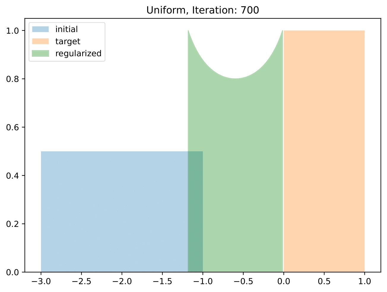
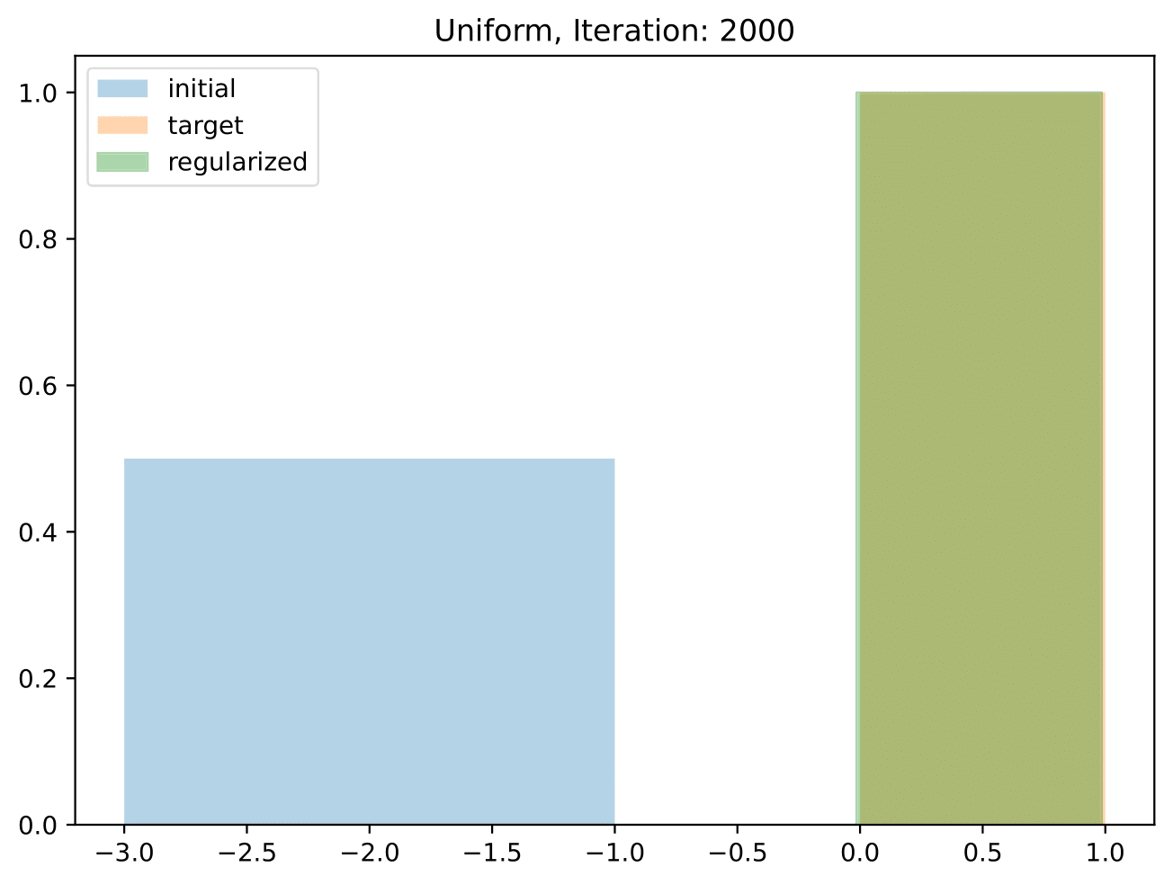
Figure 12: Regularized ${\mathcal{F}}_{\nu}^{-}$-flow between the uniform measures $\gamma_{0}\sim\mathcal{U}[-3,-1]$ and $\nu\sim\mathcal{U}[0,1]$ for $\tau=2\cdot 10^{-3}$ and "large" $\lambda=1$. The support shifts quickly towards the target.

The size of the diffusion constant $\lambda>0$ naturally determines the effective contributions of the two functionals, which are the repulsiveness of $F_{\nu}^{-}$ and the support-shifting of $F_{H,\nu}$. For small $\lambda$, the mass expands as quickly as the $F_{\nu}^{-}$-flow, while the support moves very slowly. However, for large $\lambda$, the mass expands slowly and the support shifts very quickly; see Remark 3.8 and the Figures 12, 13 in the appendix.

Figure 4: Unregularized ${\mathcal{F}}_{\nu}^{-}$-flow from $\delta_{-1}$ to $\delta_{0}$ for $\tau=10^{-3}$. The light color represents the absolute continuous part, while the dark color displays the singular part of the flow. The mass in $(-1,0)$ slowly dissipates, but never totally vanishes.

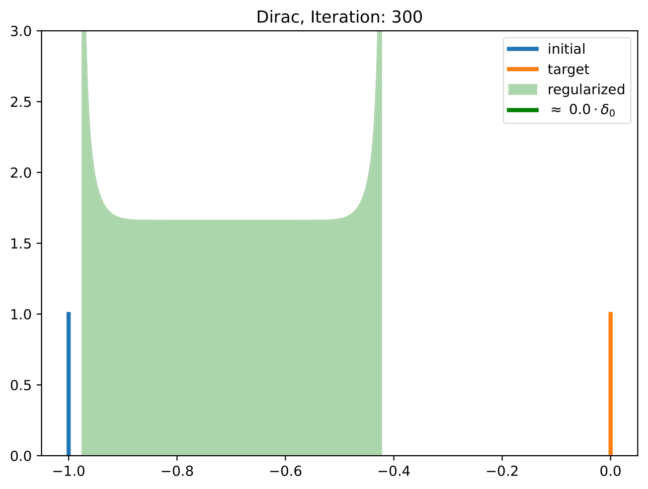
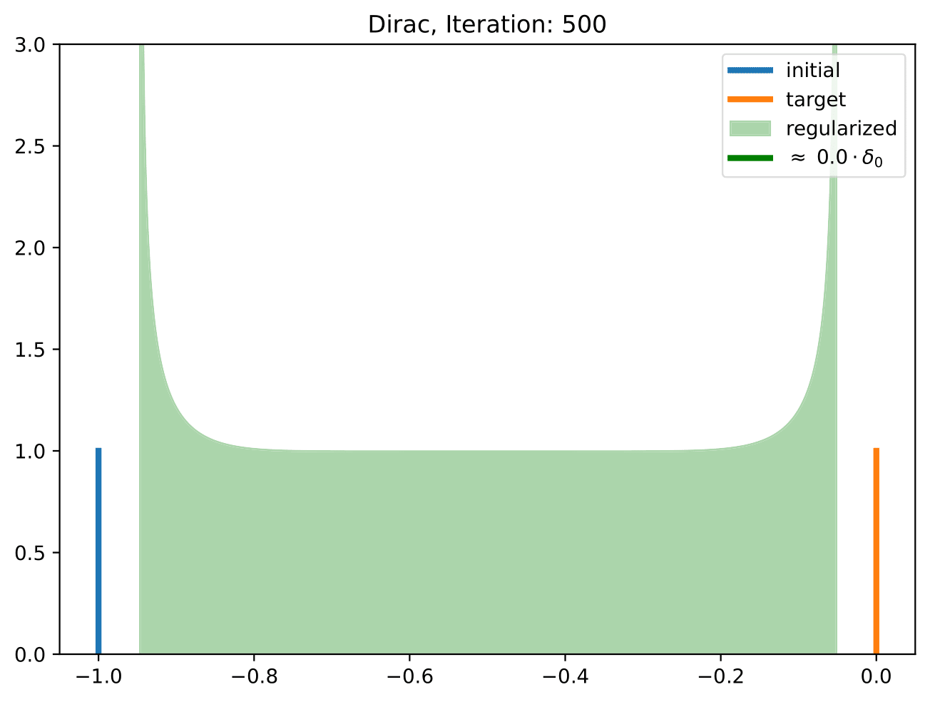
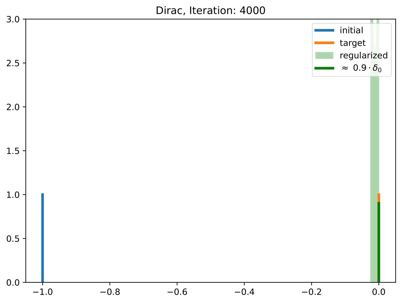
Figure 5: Regularized ${\mathcal{F}}_{\nu}^{-}$-flow from $\delta_{-1}$ to $\delta_{0}$ for $\tau=10^{-3},\,\lambda=10^{-2}$. The "horns" at the boundary of the support are of height $Q_{\nu}^{\prime}(0)^{-1}=Q_{\nu}^{\prime}(1)^{-1}=\infty$. The support shifts towards the target.

In all the remaining examples, we observe a similar behaviour: a dissipation of "sticky" mass in the unregularized ${\operatorname{\mathcal{F}}}_{\nu}^{-}$-flow; and a rectified flow of $\widetilde{\operatorname{\mathcal{F}}}_{\nu}^{-}$ where the support actually moves towards the target and the quantiles approximate the target in a smoother fashion. Hence, we are left to check whether the assumptions of Proposition 3.6 are fulfilled.

Uniform-to-Uniform:

Consider as target the uniform distribution $\nu\sim\mathcal{U}[0,1]$, and as initial measure another Uniform distribution $\gamma_{0}\sim\mathcal{U}[-3,-1]$. The corresponding quantiles are given by $Q_{\nu}(s)=s$ and $Q_{0}(s)=2s-3$, and hence satisfy the assumptions of Proposition 3.6 for any $\lambda>0$. Note that here, the Neumann boundary values $Q_{\nu}^{\prime}(0)=Q_{\nu}^{\prime}(1)=1$ instantly lead to "horn-shaped barricades" of height $1$. More precisely, by the inverse function rule, it holds

$$Q_{\nu}^{\prime}(0)=\frac{1}{f_{\nu}(Q_{\nu}(0))},\quad Q_{\nu}^{\prime}(1)=\frac{1}{f_{\nu}(Q_{\nu}(1))},$$

where $f_{\nu}$ denotes the density of $\nu$. Hence, the height of the "horns" is given by $f_{\nu}(Q_{\nu}(0)),\,f_{\nu}(Q_{\nu}(1))$, i.e., the values of the target density $f_{\nu}$ at the boundary of its support $\operatorname{supp}\nu$.
The flows of $\operatorname{\mathcal{F}}_{\nu}^{-}$, $\widetilde{\operatorname{\mathcal{F}}}_{\nu}^{-}$ and their quantile flows are depicted in Figues 6, 7 and 10, respectively.

Gaussian-to-Gaussian like:

Consider as target a suitably modified, compactly supported version of a Gaussian distribution $\widetilde{\nu}\sim\mathcal{N}(-5,1)$, and as initial measure an analogous version of $\widetilde{\gamma_{0}}\sim\mathcal{N}(5,1)$. The modifications can be chosen the following way: Since the quantile $Q_{\widetilde{\nu}}\in C^{\infty}(0,1)$ is unbounded, we cut it off outside an interval $[a,b]\subset(0,1)$, which can be chosen arbitrarily close to $(0,1)$. Then, it holds that $Q_{\widetilde{\nu}}|_{[a,b]}\in C^{\infty}([a,b])$ is smooth and bounded. Hence, we can extend $Q_{\widetilde{\nu}}|_{[a,b]}$ to a function $Q_{\nu}\in C^{3}([0,1])$ with arbitrary boundary values $Q_{\nu}^{\prime}(0),Q_{\nu}^{\prime}(1)>0$, and we can proceed the same way with $Q_{0}$. The hereby modified quantiles $Q_{\nu}$ and $Q_{0}$ hence satisfy the assumptions of Proposition 3.6 for sufficiently small $\lambda>0$. The approximate flows of $\operatorname{\mathcal{F}}_{\nu}^{-}$, $\widetilde{\operatorname{\mathcal{F}}}_{\nu}^{-}$ and their quantile flows are depicted in Figues 8, 9 and 11, respectively.

Technical implementation in the Gaussian-like case:

For simplicity, we chose to only work with the cut-off function $Q_{\widetilde{\nu}}|_{[a,b]}$ on the smaller interval $[a,b]=[1/(n+1),n/(n+1)]\subset(0,1)$, where we chose $n=1000$. Therefore, we only solve (65) on $[1/(n+1),n/(n+1)]$, where the boundary values are given by $Q_{\tilde{\nu}}^{\prime}(1/(n+1))$ and $Q_{\tilde{\nu}}^{\prime}(n/(n+1))$. As a result, the "horns" of the theoretical extension $Q_{\nu}\in C^{3}([0,1])$ are cut-off in Figure 9. But since the horns can be chosen to have small height $Q_{\nu}^{\prime}(0)^{-1},\,Q_{\nu}^{\prime}(1)^{-1}\approx 0$ anyway, this simplification is reasonable.

Figure 6: Unregularized ${\mathcal{F}}_{\nu}^{-}$-flow between the uniform measures $\gamma_{0}\sim\mathcal{U}[-3,-1]$ and $\nu\sim\mathcal{U}[0,1]$ for $\tau=2\cdot 10^{-3}$. The mass outside $\operatorname{supp}\nu$ dissipates, but never totally vanishes.

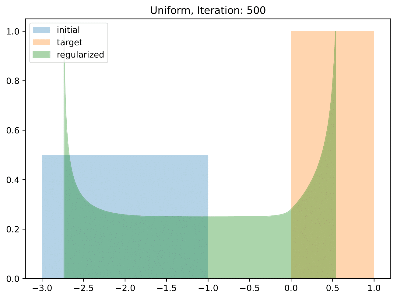
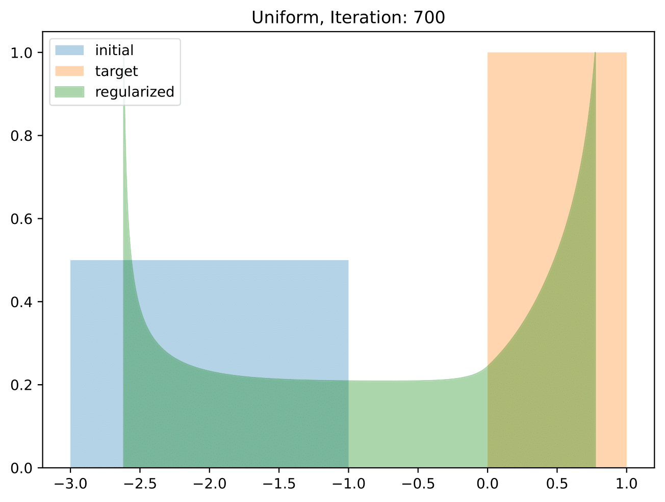
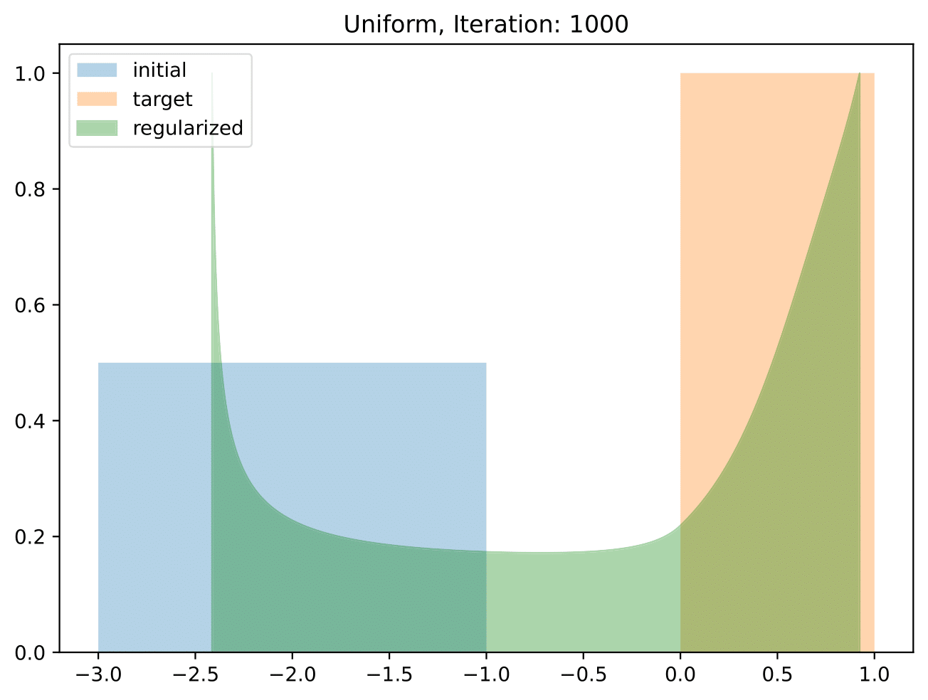
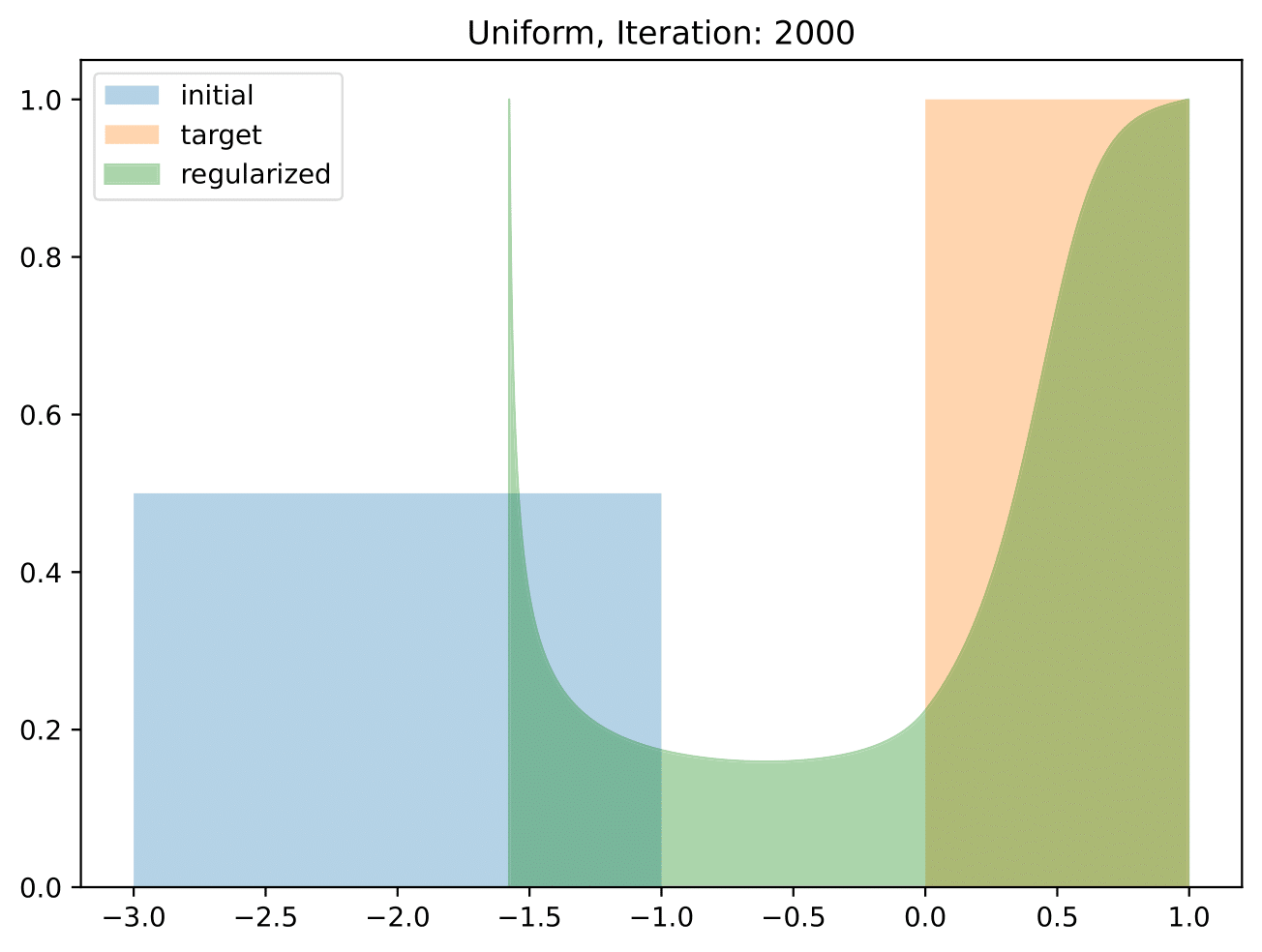
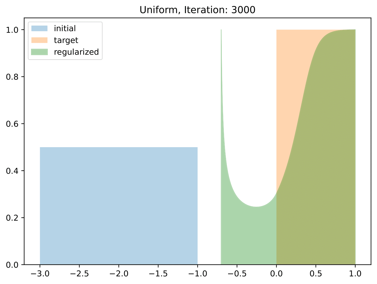
Figure 7: Regularized ${\mathcal{F}}_{\nu}^{-}$-flow between the uniform measures $\gamma_{0}\sim\mathcal{U}[-3,-1]$ and $\nu\sim\mathcal{U}[0,1]$ for $\tau=2\cdot 10^{-3}$, $\lambda=10^{-2}$. The "horns" at the boundary of the support are of height $Q_{\nu}^{\prime}(0)^{-1}=Q_{\nu}^{\prime}(1)^{-1}=1$, mirroring the target density values $f_{\nu}$ at the boundary of $\operatorname{supp}\nu$. The support shifts towards the target.

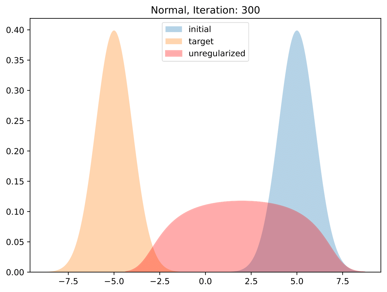
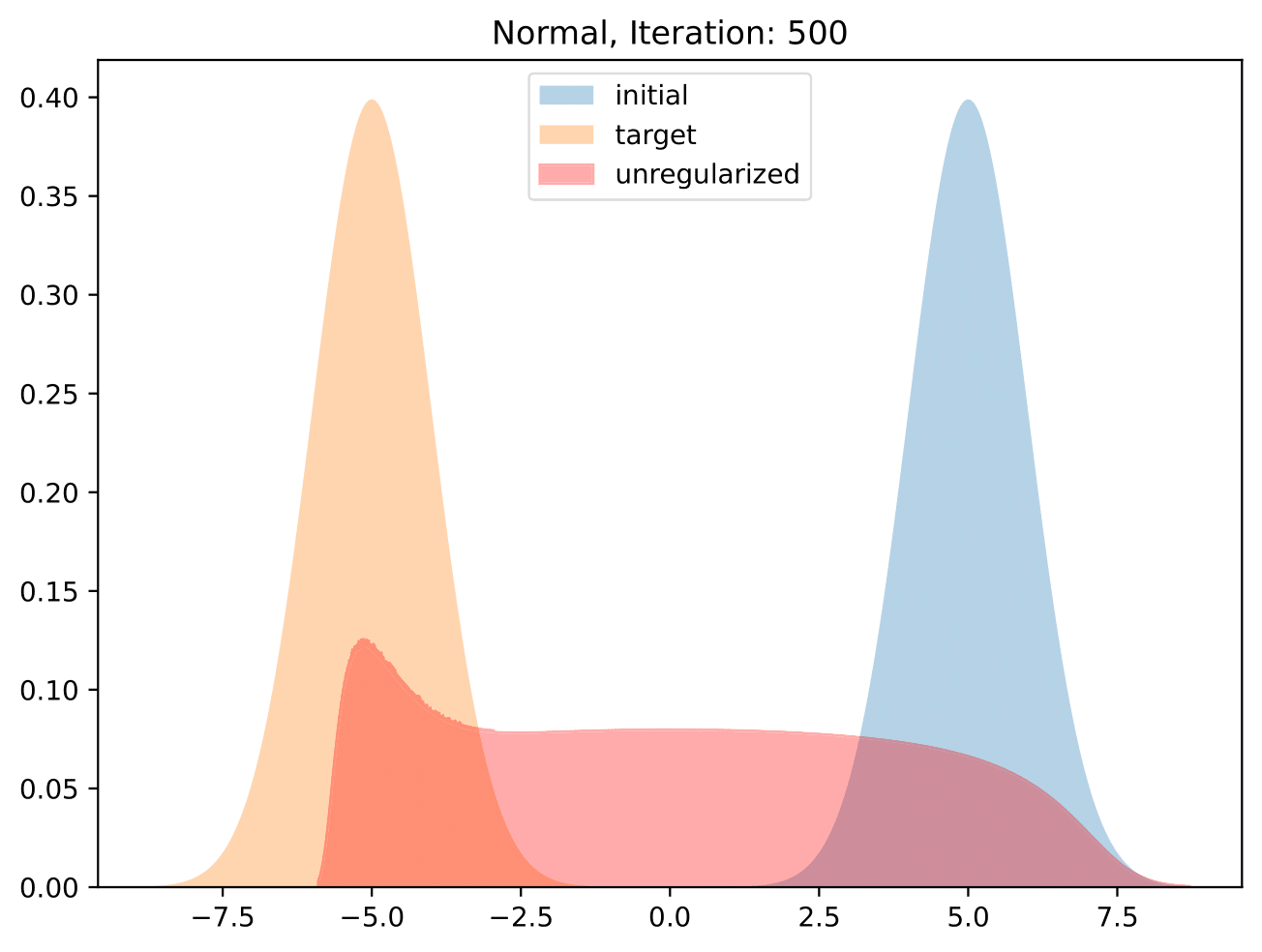
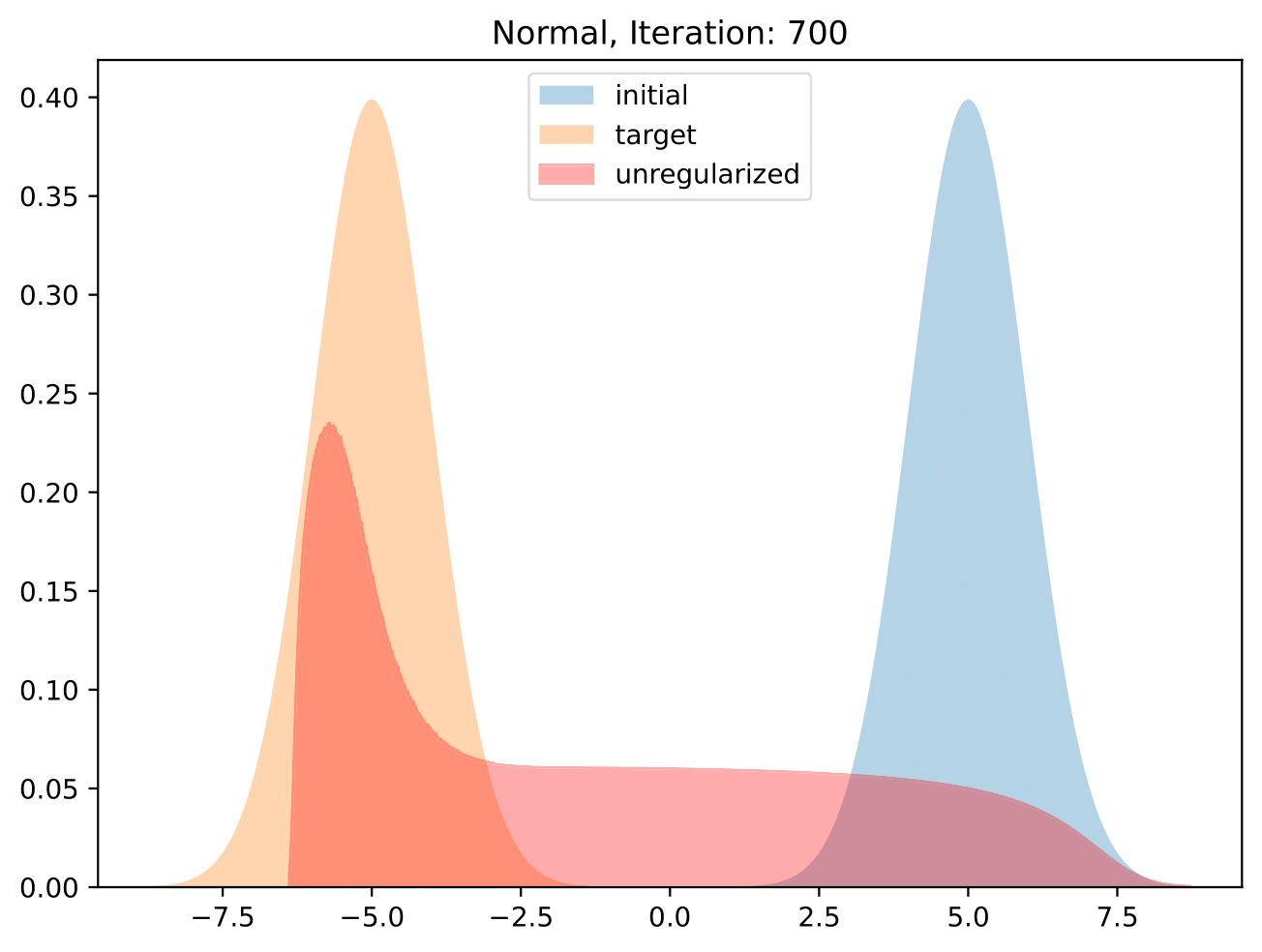
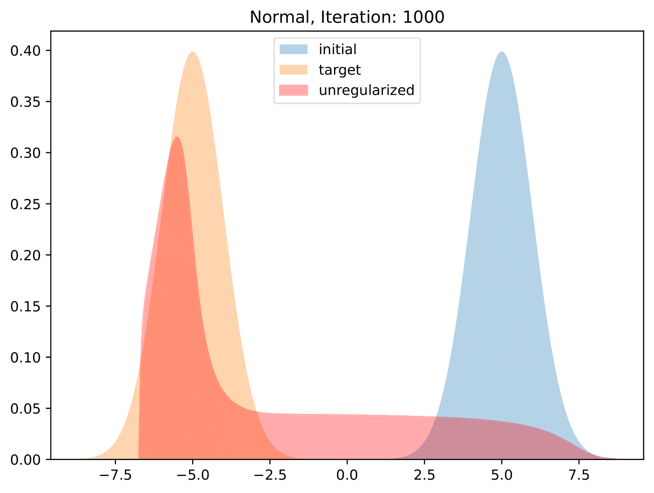
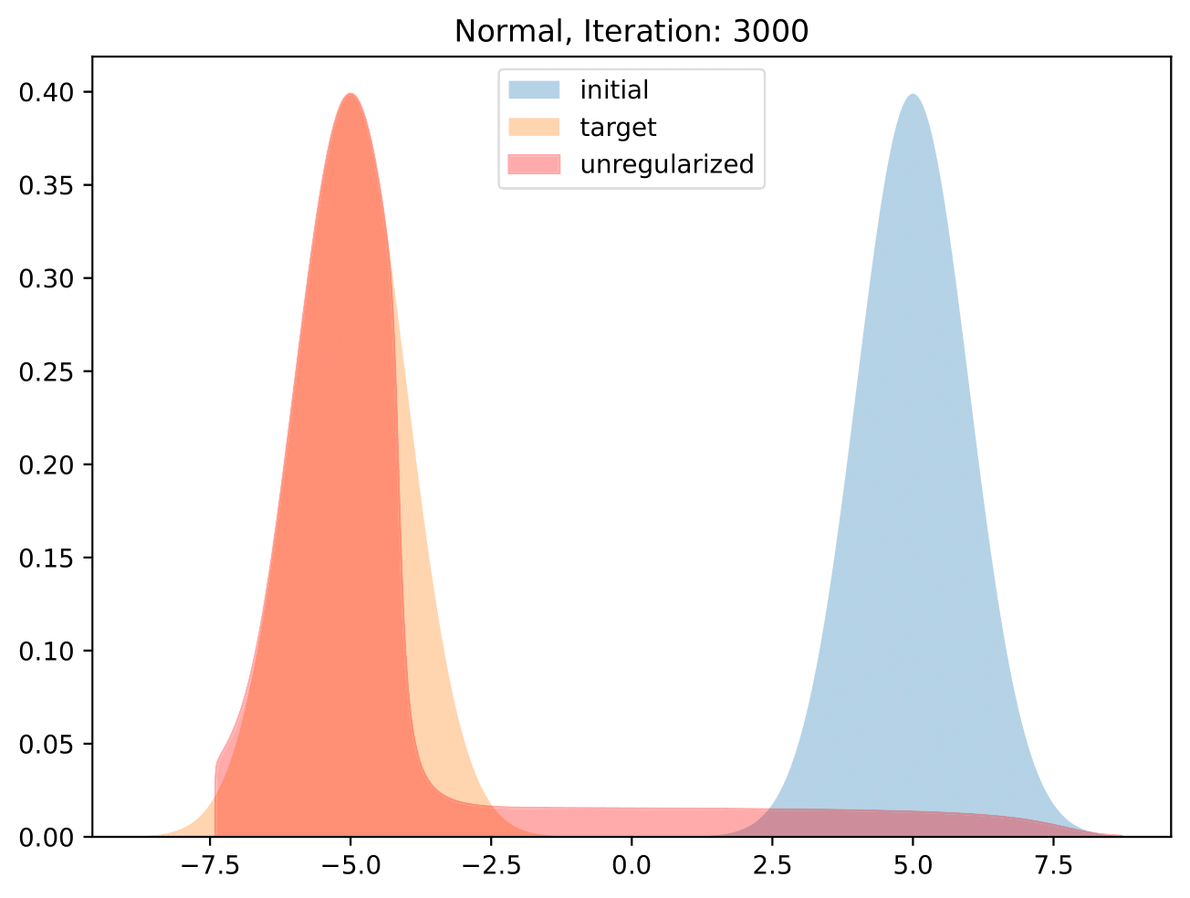
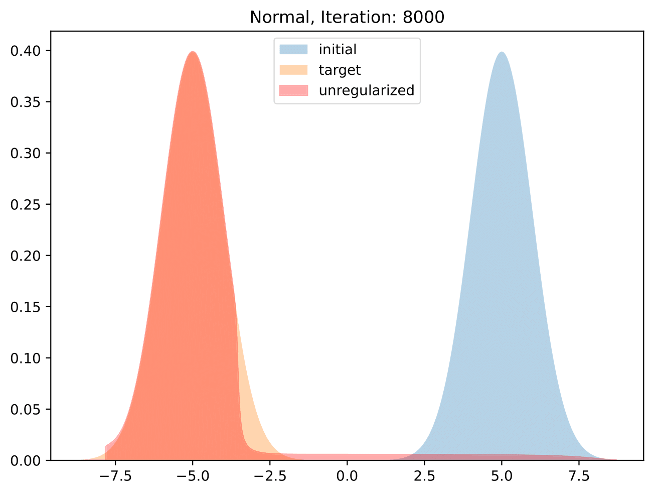
Figure 8: Unregularized ${\mathcal{F}}_{\nu}^{-}$-flow between the cut-off Gaussians $\mathcal{N}(5,1)$ and $\mathcal{N}(-5,1)$ for $\tau=10^{-2}$. The mass "sticks" to its once attained position.

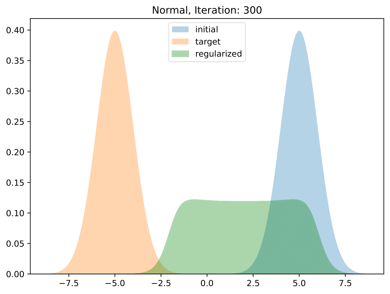
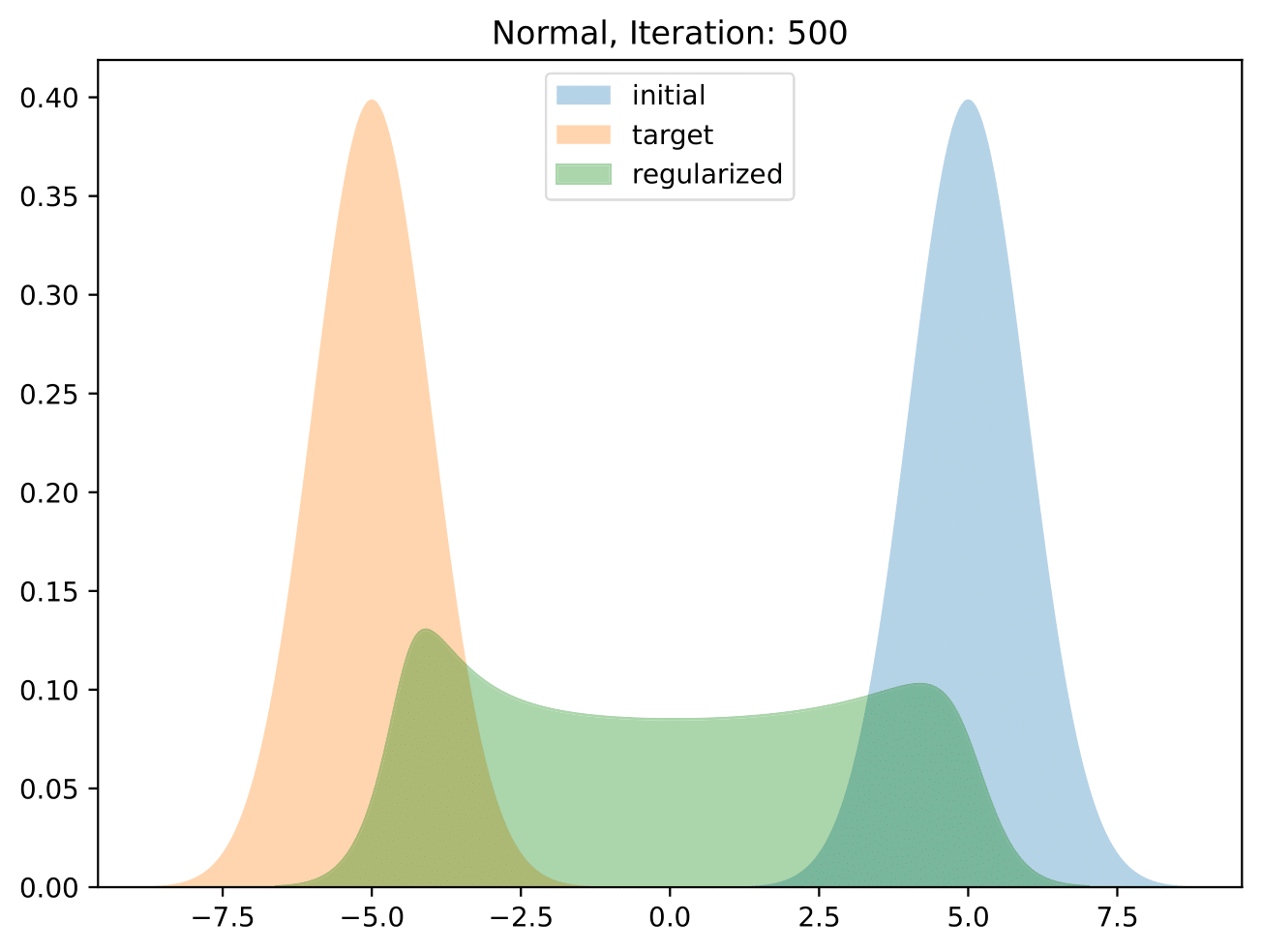
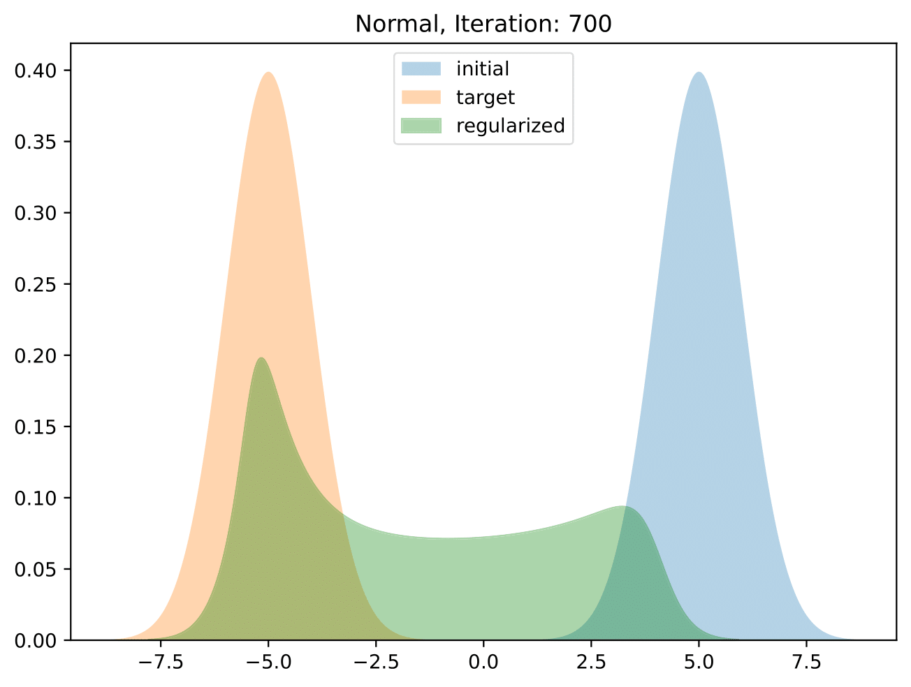
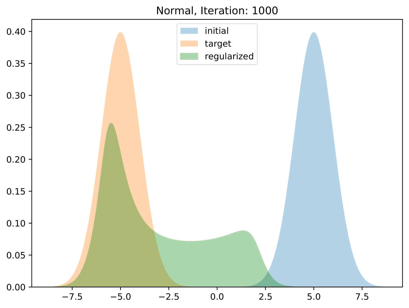
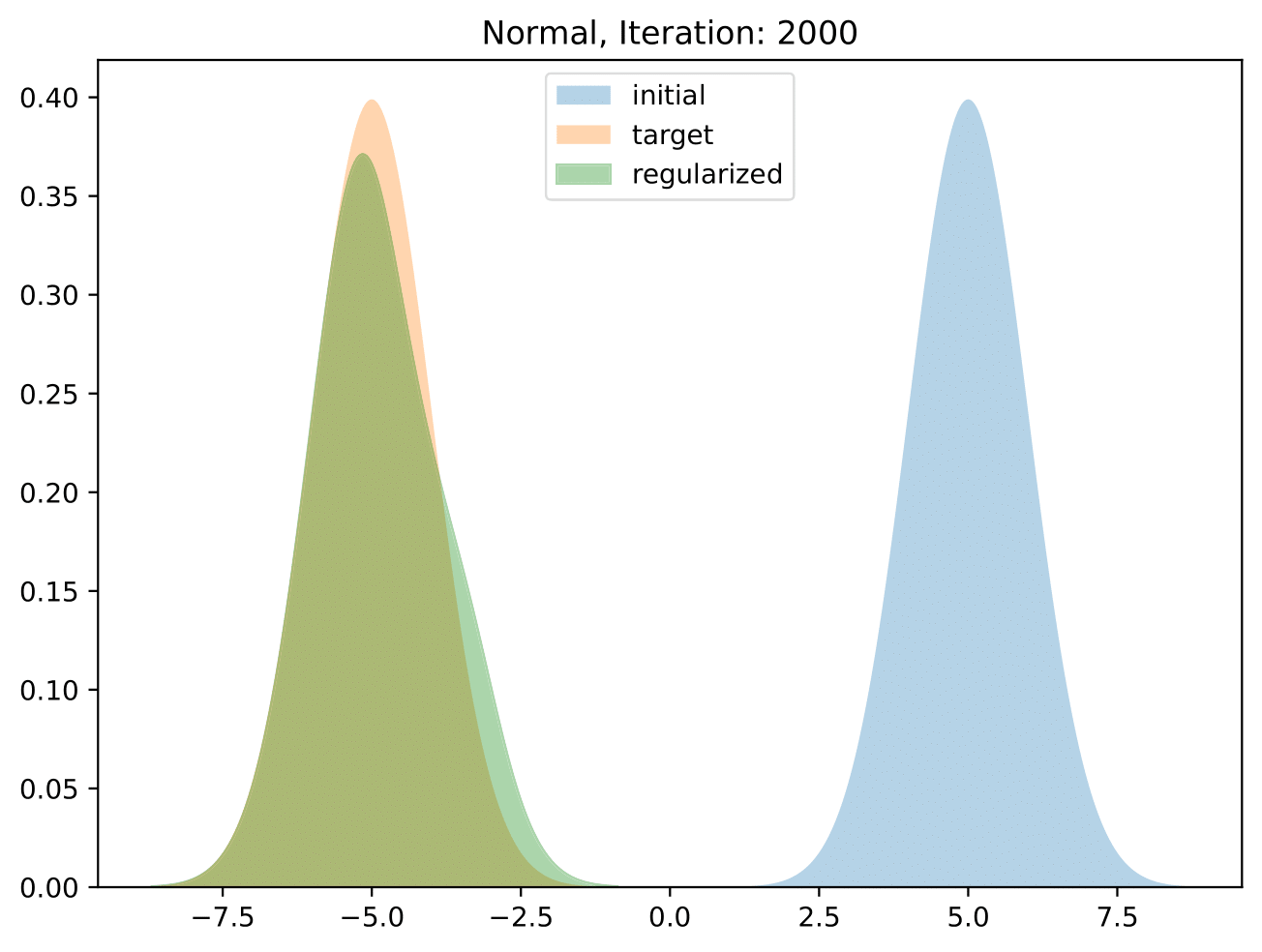
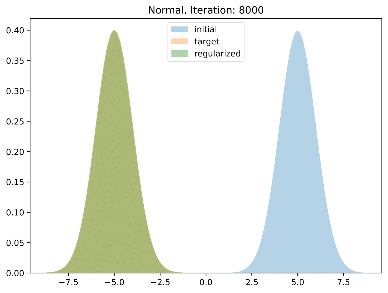
Figure 9: Regularized ${\mathcal{F}}_{\nu}^{-}$-flow between the cut-off Gaussians $\mathcal{N}(5,1)$ and $\mathcal{N}(-5,1)$ for $\tau=\lambda=10^{-2}$. Since for simplicity of implementation, we chose to only work with quantiles defined on a slightly smaller interval $[a,b]\subset(0,1)$, the "horns" at the boundary are cut off. Still, the support visibly moves in direction of the target.

Figure 10: Quantiles of the regularized and unregularized ${F}_{\nu}^{-}$-flow between uniform measures from $Q_{0}(s)=2s-3$ to $Q_{\nu}(s)=s$ with $\tau=2\cdot 10^{-3},\,\lambda=10^{-2}$.

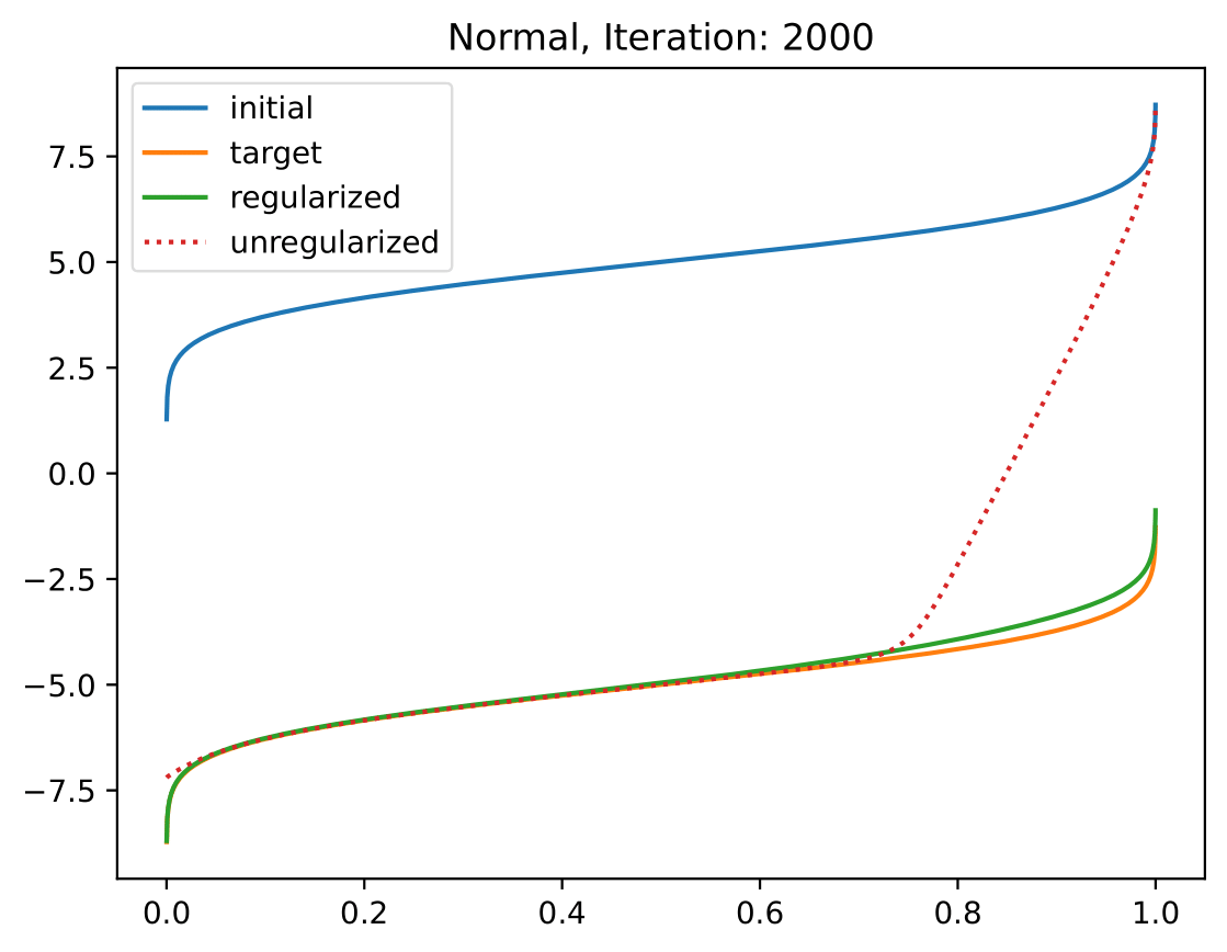
Figure 11: Quantiles of the regularized and unregularized ${F}_{\nu}^{-}$-flow between the cut-out Gaussians $\mathcal{N}(5,1)$ and $\mathcal{N}(-5,1)$ for $\tau=\lambda=10^{-2}$.

Acknowledgments.

RD acknowledges funding by the German Research Foundation (DFG) within the project STE 571/16-1.

Appendix A Appendix

A.1 Proof of Theorem 2.4

The proof is taken from [11, Theorem 3.5] with slight adjustments to our setting. Let $\gamma_{t}\coloneqq(g(t))_{\#}\Lambda_{(0,1)}$. Then, it is easy to check that $\gamma_{t}$ are probability measures in $\operatorname{\mathcal{P}}_{2}(\operatorname{\mathbb{R}})$ with quantile functions $Q_{\gamma_{t}}=g(t)$. Next, we show that $\gamma$ is locally absolutely continuous (more precisely, in ${AC}^{2}_{\rm loc}((0,\infty);\operatorname{\mathcal{P}}_{2}(\operatorname{\mathbb{R}}))$). It holds by the isometry of Theorem 2.3 that

$$W_{2}(\gamma_{t},\gamma_{s})=\|g(t)-g(s)\|_{L_{2}(0,1)}\leq\int_{s}^{t}\|g^{\prime}(\tau)\|_{L_{2}(0,1)}\mathop{}\!\mathrm{d}{\tau}\qquad\text{for all }0<s\leq t<\infty,$$

where with $m(\tau)\coloneqq\|g^{\prime}(\tau)\|_{L_{2}(0,1)}$, it holds $m\in L_{2,{\rm loc}}(0,\infty)$ by assumption. Hence, the curve $\gamma\colon[0,\infty)\to(\operatorname{\mathcal{P}}_{2}(\operatorname{\mathbb{R}}),W_{2})$ is locally absolutely continuous.

Next, we show that the optimal velocity field $v_{t}$ of $\gamma_{t}$ given by (2) fulfills $v_{t}\in-\partial\operatorname{\mathcal{F}}(\gamma_{t})$. By [1, Prop 8.4.6], for a.e. $t\in(0,\infty)$, the velocity field satisfies

$$0 =\lim_{\tau\downarrow 0}\frac{W_{2}(\gamma_{t+\tau},(\mathrm{Id}+\tau\,v_{t})_{\#}\gamma_{t})}{\tau}$$ (66)

$$=\lim_{\tau\downarrow 0}\frac{W_{2}(g(t+\tau)_{\#}\Lambda_{(0,1)},\bigl{(}g(t)+\tau\left(v_{t}\circ g(t)\right)\bigr{)}_{\#}\Lambda_{(0,1)})}{\tau}.$$ (67)

Since $v_{t}\in\mathrm{T}_{\gamma_{t}}\mathcal{P}_{2}(\operatorname{\mathbb{R}}^{d})$, there exists $\tilde{\tau}>0$ such that $(\mathrm{Id},\mathrm{Id}+\tilde{\tau}v_{t})_{\#}\gamma_{t}$ becomes an optimal transport plan. Moreover, [1, Lem 7.2.1] implies that the transport plans remain optimal for all $0<\tau\leq\tilde{\tau}$. For small $\tau>0$, the mappings $\mathrm{Id}+\tau v_{t}$ are thus optimal and, especially, monotonically increasing. Consequently, the functions $g(t)+\tau(v_{t}\circ g(t))$ are also monotonically increasing, and their left-continuous representatives are quantile functions. Employing the isometry to $L_{2}(0,1)$, we hence obtain

$$0=\lim_{\tau\downarrow 0}\Big{\|}\frac{g(t+\tau)-g(t)}{\tau}-v_{t}\circ g(t)\Big{\|}_{L_{2}(0,1)}=\|\partial_{t}g(t)-v_{t}\circ g(t)\|_{L_{2}(0,1)}.$$ (68)

Thus, since $g$ solves (11), we see that $v_{t}\circ g(t)\in-\partial F\left(g(t)\right)$ for a.e. $t$. In particular, for any $\mu\in\operatorname{\mathcal{P}}_{2}(\operatorname{\mathbb{R}})$, we obtain for a.e. $0<t<\infty$ that

$$0\,\leq\, F(Q_{\mu})-F\left(g(t)\right)+\int_{0}^{1}\left(v_{t}\circ g(t)\right)(s)\,\big{(}Q_{\mu}(s)-\left(g(t)\right)(s)\big{)}\mathop{}\!\mathrm{d}s+o(\|Q_{\mu}-g(t)\|_{L_{2}(0,1)})$$ (69)

$$=\, \mathcal{F}(\mu)-\mathcal{F}(\gamma_{t})+\int_{\operatorname{\mathbb{R}}\times\operatorname{\mathbb{R}}}v_{t}(x)\,(y-x)\mathop{}\!\mathrm{d}\pi(x,y)+o(W_{2}(\mu,\gamma_{t})),$$ (70)

where $\pi\coloneqq(g(t),Q_{\mu})_{\#}\Lambda_{(0,1)}$. By Theorem 2.3, the plan $\pi$ is optimal between $\gamma_{t}$ and $\mu$, see also [21, Thm. 2.18]. By [16, Thm. 16.1(i),(ii)], we also know that $\pi$ is unique, so that $v_{t}\in-\partial\operatorname{\mathcal{F}}(\gamma_{t})$.

Finally, the initial condition $\gamma(0+)=(g_{0})_{\#}\Lambda_{(0,1)}$ is satisfied, since $g$ is continuous at $t=0$ with $g(0)=g_{0}$. $\Box$

A.2 Material from [19]

Lemma A.1 ([19, Lemma 1.2]).

Let us assume that

$$\phi\colon L_{2}(0,1)\to(-\infty,+\infty]$$ is proper, lower semicontinuous, and (71)

$$\exists\,\tau_{*}>0:v\mapsto\varphi(v)+ \frac{1}{2\tau_{*}}|v|^{2}\text{ has compact sublevels,}$$ (72)

and the data satisfy

$$u_{0}\in\operatorname{dom}(\phi).$$ (73)

Then, $\textup{GMM}(\phi,u_{0})$ is not empty and every $u\in\textup{GMM}(\phi,u_{0})$ belongs to $H^{1}(0,T;L_{2}(0,1))$.

Theorem A.2 ([19, Theorem 3]).

Let us suppose that $\phi\colon L_{2}(0,1)\to(-\infty,+\infty]$ and $u_{0}$ satisfy the assumptions (72) and (73) of the compactness Lemma A.1, so that $\text{GMM}(\phi,u_{0})$ is not empty. If $\phi$ satisfies the following chain rule condition:

$$\text{if }v\in H^{1}(0,T;L_{2}(0,1)),\,\xi\in\, L_{2}(0,T;L_{2}(0,1)),\,\xi\in\partial\phi(v)\text{ a.e. in }(0,T),$$ (74)

$$\text{ and }\phi\circ v\text{ is bounded, then } \phi\circ v\text{ is absolutely continuous on }(0,T)\text{ and }$$ (75)

$$\frac{d}{dt}\phi(v(t))= \langle\xi(t),{v}^{\prime}(t)\rangle\text{ for a.e. }t\in(0,T),$$ (76)

then, every $u\in\textup{GMM}(\phi,u_{0})$ is a solution in $H^{1}(0,T;L_{2}(0,1))$ to

$$\begin{cases}u^{\prime}(t)+\partial_{l}\phi(u(t))\ni 0,&\text{a.e. in }(0,T),\\ u(0)=u_{0}.&\end{cases}$$ (77)

Remark A.3 ([19, Remark 1.9]).

Assume $\psi_{1}$ and $\psi_{2}$ are convex and

$$\phi=\psi_{1}-\psi_{2}\quad\text{in }\operatorname{dom}(\phi) ,\text{ where}$$ (78)

$$\psi_{1},\psi_{2}\colon\operatorname{dom}(\phi)\to\mathbb{R}\text{ are lsc and convex} ,~{}\operatorname{dom}(\partial\psi_{1})\subset\operatorname{dom}(\partial\psi_{2}).$$ (79)

Then, $\phi$ satisfies the chain rule (75).

A.3 Influence of different values of the regularization parameter $\lambda$

References

• [1] L. Ambrosio, N. Gigli, and G. Savare. Gradient Flows. Lectures in Mathematics ETH Zürich. Birkhäuser, Basel, 2nd edition, 2008.
• [2] M. Arbel, A. Korba, A. Salim, and A. Gretton. Maximum mean discrepancy gradient flow. In Advances in Neural Information Processing Systems, volume 32, 2019.
• [3] H. Attouch. Familles d’opérateurs maximaux monotones et mesurabilité. Annali di Matematica Pura ed Applicata, 120(4):35–111, 1979.
• [4] V. Barbu. Nonlinear Differential Equations of Monotone Types in Banach Spaces. Springer Science & Business Media, 2010.
• [5] A. Bobrowski and R. Rudnicki. On convergence and asymptotic behaviour of semigroups of operators. Philosophical Transactions of the Royal Society A, 378, 2020.
• [6] G. A. Bonaschi, J. A. Carrillo, M. Di Francesco, and M. A. Peletier. Equivalence of gradient flows and entropy solutions for singular nonlocal interaction equations in 1d. ESAIM: Control, Optimisation and Calculus of Variations, 21(2):414–441, 2015.
• [7] S. Boufadène and F.-X. Vialard. On the global convergence of Wasserstein gradient flow of the Coulomb discrepancy. arXiv preprint arXiv:2312.00800, 2023.
• [8] H. Brezis. Operateurs Maximaux Monotones. North-Holland Mathematics Studies, 1973.
• [9] H. Brezis and A. Pazy. Convergence and approximation of semigroups of nonlinear operators in Banach spaces. Journal of Functional Analysis, 9:63–74, 1972.
• [10] Y. Chen, D. Z. Huang, J. Huang, S. Reich, and A. M. Stuart. Sampling via gradient flows in the space of probability measures. arXiv preprint arXiv:2310.03597, 2023.
• [11] R. Duong, V. Stein, R. Beinert, J. Hertrich, and G. Steidl. Wasserstein gradient flows of MMD functionals with distance kernel and Cauchy problems on quantile functions. arXiv preprint arXiv:2408.07498, 2024.
• [12] P. Hagemann, J. Hertrich, F. Altekrüger, R. Beinert, J. Chemseddine, and G. Steidl. Posterior sampling based on gradient flows of the MMD with negative distance kernel. In International Conference on Learning Representations, 2024.
• [13] J. Hertrich, R. Beinert, M. Gräf, and G. Steidl. Wasserstein gradient flows of the discrepancy with distance kernel on the line. In International Conference on Scale Space and Variational Methods in Computer Vision, pages 431–443. Springer, 2023.
• [14] J. Hertrich, M. Gräf, R. Beinert, and G. Steidl. Wasserstein steepest descent flows of discrepancies with Riesz kernels. Journal of Mathematical Analysis and Applications, 531(1):127829, 2024.
• [15] R. Laumont, V. Bortoli, A. Almansa, J. Delon, A. Durmus, and M. Pereyra. Bayesian imaging using plug & play priors: when Langevin meets Tweedie. SIAM Journal on Imaging Sciences, 15(2):701–737, 2022.
• [16] F. Maggi. Optimal Mass Transport on Euclidean Spaces. Cambridge Studies in Advanced Mathematics. Cambridge University Press, 2023.
• [17] R. R. Phelps. Convex functions, Monotone Operators and Differentiability (2nd edition). Springer, Berlin, Heidelberg, New York, 1993.
• [18] R. T. Rockafellar and J. O. Royset. Random variables, monotone relations, and convex analysis. Mathematical Programming, 148:297–331, 2014.
• [19] R. Rossi and G. Savaré. Gradient flows of non convex functionals in Hilbert spaces and applications. ESAIM: Control, Optimisation and Calculus of Variations, 12:564–614, 2006.
• [20] T. Teuber, G. Steidl, P. Gwosdek, C. Schmaltz, and J. Weickert. Dithering by differences of convex functions. SIAM Journal on Imaging Sciences, 4(1):79–108, 2011.
• [21] C. Villani. Topics in Optimal Transportation. Number 58 in Graduate Studies in Mathematics. American Mathematical Society, Providence, 2003.
• [22] C. Villani. Optimal Transport. Springer, Berlin, 2009.