Analysis of the Streamline Upwind/Petrov Galerkin Method Applied to the Solution of Optimal Control Problems

Abstract

We study the effect of the streamline upwind/Petrov Galerkin (SUPG) stabilized finite element method on the discretization of optimal control problems governed by linear advection-diffusion equations. We compare two approaches for the numerical solution of such optimal control problems. In the discretize-then-optimize approach the optimal control problem is first discretized, using the SUPG method for the discretization of the advection-diffusion equation, and then the resulting finite dimensional optimization problem is solved. In the optimize-then-discretize approach one first computes the infinite dimensional optimality system, involving the advection-diffusion equation as well as the adjoint advection-diffusion equation, and then discretizes this optimality system using the SUPG method for both the original and the adjoint equations. These approaches lead to different results. The main result of this paper are estimates for the error between the solution of the infinite dimensional optimal control problem and their approximations computed using the previous approaches. For a class of problems prove that the optimize-then-discretize approach has better asymptotic convergence properties if finite elements of order greater than one are used. For linear finite elements our theoretical convergence results for both approaches are comparable, except in the zero diffusion limit where again the optimize-then-discretize approach seems favorable. Numerical examples are presented to illustrate some of the theoretical results.

Key words Optimal control, discretization, error estimates, stabilized finite elements.

AMS subject classifications 49M25, 49K20, 65N15, 65J10

1 Introduction

This paper is concerned with the accuracy of numerical solutions of optimal control problems governed by the advection-diffusion equation. Specifically, we are interested in the effect of the streamline upwind/Petrov Galerkin (SUPG) stabilized finite element method on the discretization of the optimal control problem. To be more precise, we consider the linear quadratic optimal control problem

$$\min\frac{1}{2}\int_{\Omega}(y(x)-\widehat{y}(x))^{2}dx+\frac{\omega}{2}\int_{\Omega}u^{2}(x)dx$$ (1.1)

subject to

$$-\epsilon\Delta y(x)+\mathbf{c}(x)\cdot\nabla y(x)+r(x)y(x) =f(x)+u(x), x \in\Omega,\;$$ (1.2a)

$$y(x) =d(x), x \in\Gamma_{d},$$ (1.2b)

$$\epsilon\frac{\partial}{\partial\mathbf{n}}y(x) =g(x), x \in\Gamma_{n},$$ (1.2c)

where $\Gamma_{d}\cap\Gamma_{n}=\emptyset$, $\Gamma_{d}\cup\Gamma_{n}=\partial\Omega$, $\mathbf{c},d,f,g,r,\widehat{y}$ are given functions, $\epsilon,\omega>0$ are given scalars, and $\mathbf{n}$ denotes the outward unit normal. Assumptions on these data that ensure the well-posedness of the problem will be given in the next section.

For advection dominated problems the standard Galerkin finite element method applied to the state equation (1.2) produces strongly oscillatory solutions, unless the mesh size $h$ is chosen sufficiently small relative to $\epsilon/\|\mathbf{c}(x)\|$, $x\in\Omega$. To produce better approximations to the solution of (1.2) for modest mesh sizes, various augmentations of the standard Galerkin finite element method have been proposed. For an overview see [11, 12, 13]. In this paper we focus on the streamline upwind/Petrov Galerkin (SUPG) method of Hughes and Brooks [2]. The SUPG method adds to the weak form of the state equation (1.2) a term with the properties that (a) the weak form of the modification has better stability properties than the bilinear form associated with (1.2) and (b) the added term evaluated at the exact solution of (1.2) vanishes. Because of these properties the SUPG method is called a strongly consistent stabilization method [12].

For the numerical solution of the optimal control problem there are at least two approaches. In the first approach, called the optimize-then-discretize approach, one first derives the optimality conditions for (1.1), (1.2). In Section (2.1) we will see that the optimality conditions consist of the state equation (1.2), the adjoint partial differential equation (PDE)

$$-\epsilon\Delta\lambda(x)-\mathbf{c}(x)\cdot\nabla\lambda(x)+(r(x)-\nabla\cdot\mathbf{c}(x))\lambda(x) =-(y(x)-\hat{y}(x)), x \in\Omega,$$ (1.3a)

$$\lambda(x) =0, x \in\Gamma_{d},$$ (1.3b)

$$\epsilon\frac{\partial}{\partial\mathbf{n}}\lambda(x)+\mathbf{c}(x)\cdot\mathbf{n}(x)\;\lambda(x) =0, x \in\Gamma_{n}$$ (1.3c)

and the gradient equation

$$\lambda(x)=\omega u(x)\qquad x\in\Omega.$$ (1.4)

Then one discretizes each equation (1.2), (1.3) and (1.4), using possibly different discretization schemes for each one. Since the adjoint equation (1.3) is also an advection-diffusion equation, but with advection $-\mathbf{c}$, we discretize it using the SUPG method. If we proceed this way, the optimize-then-discretize approach leads to a discretization of the optimality system (1.2), (1.3), (1.4) that is strongly consistent. However, this discretization of the optimality system (1.2), (1.3), (1.4) leads to a nonsymmetric linear system, which implies that there is no finite dimensional optimization problem for which this discretization of (1.2), (1.3), (1.4) is the optimality system. The details of the optimize-then-discretize approach will be discussed in Section 2.4. In the other approach for the numerical solution of (1.1), (1.2) called the discretize-then-optimize approach, one first discretizes the state equation using SUPG and the objective function and then solves the resulting finite dimensional optimization problem. The optimality conditions of this finite dimensional optimization problem contain equations, which we call the discrete adjoint equation and the discrete gradient equation, that can be viewed as discretizations of (1.3) and (1.4), respectively. The SUPG stabilization term added to the state equation (1.2) produces a contribution to the discrete adjoint equation and to the discrete gradient equation. This contribution to the discrete adjoint equation has a stabilizing effect, but the discrete adjoint equation is in general not a strongly consistent stabilization method for (1.3). We will give a detailed discussion of the optimize-then-discretize approach in Section 2.3. The main goal of this paper is to derive estimates of the error between the solution $y,u,\lambda$ of the infinite dimensional optimality system (1.2), (1.3), (1.4) and their approximations computed using both, the discretize-then-optimize as well as the optimize-then-discretize approach. Such error estimates will be provided in Section 4. Section 5 contains a few numerical results that illustrate our theoretical findings.

We will see that even in our simple model problem (1.1), (1.2) differences can arise between the discretize-then-optimize and the optimize-then-discretize approach. It is important to understand and analyze these to better assess the implication of numerical solution approaches to much more complicated optimal control or optimal design problems that involve nonlinear state equations solved using stabilization techniques. We also note that the general issues described here for the SUPG stabilization also arise when other stabilizations are used, such as the Galerkin/Least-squares (GLS) method of Hughes, Franca and Hulbert [6] and the stabilization method of Franca, Frey and Hughes [4].

Throughout this paper we use the following notation for norms and inner products. We define $\langle f,g\rangle_{G}=\int_{G}f(x)g(x)dx$, $\|v\|_{0,\infty,G}=\mbox{ ess sup}_{x\in G}|v(x)|$ or $\|{\bf v}\|_{0,\infty,G}=\mbox{ ess sup}_{x\in G}\sqrt{\sum_{i}v_{i}(x)^{2}}$ for vector valued ${\bf v}$, and

$$\|v\|_{k,G}=\left(\sum_{|\alpha|\leq k}\int_{G}(\partial^{\alpha}v(x))^{2}dx\right)^{1/2},\qquad|v|_{k,G}=\left(\sum_{|\alpha|=k}\int_{G}(\partial^{\alpha}v(x))^{2}dx\right)^{1/2},$$

where $G\subset\Omega\subset I\!\!R^{d}$ or $G\subset\partial\Omega$ and $\alpha\in I\!\!N_{0}^{d}$ is a multi-index, $|\alpha|=\sum_{i=1}^{d}\alpha_{i}$, and $\partial^{\alpha}=\partial^{\alpha_{1}}\ldots\partial^{\alpha_{d}}$. If $G=\Omega$ we omit $G$ and simply write $\langle f,g\rangle$, etc.

2 A Model Problem

2.1 Existence, Uniqueness and Characterization of Optimal Controls

We define the state and control space

$$Y=\left\{{y\in H^{1}(\Omega)}\,:~{}{y=d\mbox{ on }\Gamma_{d}}\right\},\quad U=L^{2}(\Omega)$$ (2.1)

and space of test functions

$$V=\left\{{v\in H^{1}(\Omega)}\,:~{}{v=0\mbox{ on }\Gamma_{d}}\right\}.$$ (2.2)

The weak form of the state equations (1.2) is given by

$$a(y,v)+b(u,v)=\langle f,v\rangle+\langle g,v\rangle_{\Gamma_{n}}\quad\forall v\in V,$$ (2.3)

where

$$a(y,v) = \int_{\Omega}\epsilon\nabla y(x)\cdot\nabla v(x)+\mathbf{c}(x)\cdot\nabla y(x)v(x)+r(x)y(x)v(x)dx,$$ (2.4)

$$b(u,v) = -\int_{\Omega}u(x)v(x)dx,$$ (2.5)

$$\langle f,v\rangle = \int_{\Omega}f(x)v(x)dx,\qquad\langle g,v\rangle_{\Gamma_{n}}=\int_{\Gamma_{n}}g(x)v(x)dx.$$ (2.6)

We are interested in the solution of the optimal control problem

minimize $$\frac{1}{2}\|y-\widehat{y}\|_{0}^{2}+\frac{\omega}{2}\|u\|_{0}^{2},$$ (2.7a)

subject to $$a(y,v)+b(u,v)=\langle f,v\rangle+\langle g,v\rangle_{\Gamma_{n}}\quad\forall v\in V,$$

$$y\in Y,u\in U.$$

We assume that

$$f,\widehat{y}\in L^{2}(\Omega),\mathbf{c}\in\left(W^{1,\infty}(\Omega)\right)^{2},r\in L^{\infty}(\Omega),d\in H^{3/2}(\Gamma_{d}),g\in H^{1/2}(\Gamma_{n}),\omega>0,\epsilon>0,$$ (2.8a)

$$\Gamma_{n}\subset\left\{{x\in\partial\Omega}\,:~{}{\mathbf{c}(x)\cdot\mathbf{n}(x)\geq 0}\right\}$$ (2.8b)

and

$$r(x)-\mbox{$\frac{1}{2}$}\nabla\cdot\mathbf{c}(x)\geq r_{0}>0\mbox{ a.e. in }\Omega.$$ (2.8c)

If $$\Gamma_{d}\not=\emptyset \alpha>0 |y|_{1}\leq\alpha\|y\|_{1} y\in V$$, there exists such that for all and (2.8c) can be replaced by

$$r(x)-\mbox{$\frac{1}{2}$}\nabla\cdot\mathbf{c}(x)\geq r_{0}\geq 0\mbox{ a.e. in }\Omega.$$ (2.8d)

For the well-posedness of the optimal control problem it is sufficient to impose fewer regularity requirements on the coefficient functions than those stated in (2.8a). We assume (2.8a) to establish convergence estimates for the SUPG finite element method.

Under the assumptions (2.8), the bilinear form $a$ is continuous on $V\times V$ and $V$-elliptic. In fact, $a(y,y)\geq\epsilon\|\nabla y\|_{0}^{2}+r_{0}\|y\|_{0}^{2}$ for all $y\in V$ (e.g., [12, p. 165] or [11, Sec. 2.5]). Hence the theory in [10, Sec. II.1] guarantees the existence of a unique solution $(y,u)\in Y\times U$ of (2.7).

Theorem 2.1

If (2.8) are satisfied, the optimal control problem (2.7) has a unique solution $(y,u)\in Y\times U$.

The theory in [10, Sec. II.1] also provides necessary and sufficient optimality conditions, which can be best described using the Lagrangian

$$L(y,u,\lambda)=\frac{1}{2}\|y-\widehat{y}\|_{0}^{2}+\frac{\omega}{2}\|u\|_{0}^{2}+a(y,\lambda)+b(u,\lambda)-\langle f,\lambda\rangle-\langle g,v\rangle_{\Gamma_{n}}.$$ (2.9)

The necessary and, for our model problem, sufficient optimality conditions can be obtained by setting the partial Fréchet-derivatives of (2.9) with respect to states $y$, controls $u$ and adjoints $\lambda$ equal to zero. This gives the following system consisting of
the adjoint equation

$$a(\psi,\lambda)=-\langle y-\hat{y},\psi\rangle\quad\forall\psi\in V,$$ (2.10a)

the gradient equation

$$b(w,\lambda)+\omega\langle u,w\rangle=0\quad\forall w\in U,$$ (2.10b)

and the state equation

$$a(y,v)+b(u,v)=\langle f,v\rangle+\langle g,v\rangle_{\Gamma_{n}}\quad\forall v\in V.$$ (2.10c)

The gradient equation (2.10b) simply means that $\lambda(x)=\omega u(x)$, $x\in\Omega$ (cf. (1.4)) and (2.10a) is the weak form of (1.3).

The adjoint equation (1.3) is also an advection-diffusion equation, but advection is now given by $-\mathbf{c}$ and the reaction term is $r-\nabla\cdot\mathbf{c}$.

The convergence theory for SUPG methods requires that the solution $y,u,\lambda$ is more regular than indicated by Theorem 2.1. This can be guaranteed if the problem data are such that the state equation (1.2) and adjoint equation (1.3) admit more regular solutions. This motivates our regularity assumptions (2.8a) on the data. The following result is an application of [5, Thm. 2.4.2.5] to (1.2) and (1.3).

Theorem 2.2

Let $\Omega$ be a bounded open subset of $I\!\!R^{n}$ with a $C^{1,1}$ boundary and $\Gamma_{d}=\partial\Omega$. If the assumption (2.8a) is satisfied and $r\geq r_{0}>0$ a.e., then the unique solution of the optimal control problem (2.7) and the associated adjoint satisfy $y\in H^{2}(\Omega),u\in H^{2}(\Omega),\lambda\in H^{2}(\Omega)$.

2.2 Discretization of the State Equations

For the discretization of the state equation we use conforming finite elements. We let $\{\mathcal{T}_{h}\}_{h>0}$ be a family of quasi-uniform triangulations of $\Omega$ [3]. To approximate the state equation we use the spaces

$$\begin{array}[]{rcl}Y_{h}&=&\left\{{y_{h}\in Y}\,:~{}{y_{h}|_{T}\in P_{k}(T)\mbox{ for all }T\in\mathcal{T}_{h}}\right\},\\ V_{h}&=&\left\{{v_{h}\in V}\,:~{}{v_{h}|_{T}\in P_{k}(T)\mbox{ for all }T\in\mathcal{T}_{h}}\right\},\quad k\geq 1.\end{array}$$ (2.11)

For advection dominated problems the standard Galerkin method applied to the state equation (2.3) produces strongly oscillatory approximations, unless the mesh size $h$ is chosen sufficiently small relative to $\epsilon/\|\mathbf{c}\|_{0,\infty}$. To obtain approximate solutions of better quality on coarser meshes, various stabilization techniques have been proposed. For an overview see [12, Secs. 8.3.2,8.4] or [13, Sec.3.2]. We are interested in the streamline upwind/Petrov Galerkin (SUPG) method of Hughes and Brooks [2]. The SUPG method computes an approximation $y_{h}\in Y_{h}$ of the solution $y$ of the state equation (2.7) by solving

$$a_{h}^{\sf s}(y_{h},v_{h})+b_{h}^{\sf s}(u_{h},v_{h})=\langle f,v_{h}\rangle_{h}^{\sf s}+\langle g,v_{h}\rangle_{\Gamma_{n}}\quad\forall v_{h}\in V_{h},$$ (2.12)

where

$$a_{h}^{\sf s}(y,v_{h}) = a(y,v_{h})+\sum_{T_{e}\in\mathcal{T}_{h}}\tau_{e}\langle-\epsilon\Delta y+\mathbf{c}\cdot\nabla y+ry,\mathbf{c}\cdot\nabla v_{h}\rangle_{T_{e}},$$ (2.13a)

$$b_{h}^{\sf s}(u,v_{h}) = -\int_{\Omega}u(x)v_{h}(x)dx-\sum_{T_{e}\in\mathcal{T}_{h}}\tau_{e}\langle u,\mathbf{c}\cdot\nabla v_{h}\rangle_{T_{e}},$$ (2.13b)

$$\langle f,v_{h}\rangle_{h}^{\sf s} = \langle f,v_{h}\rangle+\sum_{T_{e}\in\mathcal{T}_{h}}\tau_{e}\langle f,\mathbf{c}\cdot\nabla v_{h}\rangle_{T_{e}}.$$ (2.13c)

In (2.15) the superscript ${\sf s}$ is used to indicate that the stabilization method is applied to the state equation, i.e., all parameters in the stabilization method are based on information from the state equation only. The reason for the additional superscript ${\sf s}$ will become apparent in Section 2.4. The addition of the term $\sum_{T_{e}\in\mathcal{T}_{h}}\tau_{e}\langle-\epsilon\Delta y+\mathbf{c}\cdot\nabla y+ry,\mathbf{c}\cdot\nabla v_{h}\rangle_{T_{e}}$ to $a(y,v_{h})$ introduces additional element wise diffusion $\langle\mathbf{c}\cdot\nabla y,\mathbf{c}\cdot\nabla v_{h}\rangle_{T_{e}}$ and enhances the stability properties of $a(y,v_{h})$ (see Lemma 4.1 below). The terms in (2.12) added to the standard Galerkin formulation are such that the exact solution $y$ of (1.2) satisfies (2.12), provided $y\in H^{2}(T_{e})$, $T_{e}\in{\cal T}_{h}$. We will review the error estimates for the SUPG method in Section 4.1.

2.3 Discretization of the Optimization Problem

A frequently used approach for the numerical solution of an optimal control problem is to discretize the optimal control problem and to solve the resulting nonlinear programming problem using a suitable optimization algorithm. This is also called the discretize-then-optimize approach. In this scenario, the discretization of the optimal control problem typically follows discretization techniques used for the governing state equations.

In our problem we select the spaces (2.11) for the discretization of the state and

$$U_{h}=\left\{{u_{h}\in U}\,:~{}{u_{h}|_{T}\in P_{m}(T)\mbox{ for all }T\in\mathcal{T}_{h}}\right\},\quad m\geq 0,$$ (2.14)

for the control. To discretize the state equation, we apply the SUPG method. The discretized optimal control problem is given by

minimize $$\frac{1}{2}\|y_{h}-\widehat{y}\|_{0}^{2}+\frac{\omega}{2}\|u_{h}\|_{0}^{2},$$ (2.15a)

subject to $$a_{h}^{\sf s}(y_{h},v_{h})+b_{h}^{\sf s}(u_{h},v_{h})=\langle f,v_{h}\rangle_{h}^{\sf s}+\langle g,v_{h}\rangle_{\Gamma_{n}}\quad\forall v_{h}\in V_{h},$$

$$y_{h}\in Y_{h},\quad u_{h}\in U_{h},$$

where $a_{h}^{\sf s}(y,v_{h})$, $b_{h}^{\sf s}(u,v_{h})$, $\langle f,v_{h}\rangle_{h}^{\sf s}$ are defined in (2.13).

The Lagrangian for the discretized problem (2.15) is given by

$$L_{h}(y_{h},u_{h},\lambda_{h})=\frac{1}{2}\|y_{h}-\widehat{y}\|_{0}^{2}+\frac{\omega}{2}\|u_{h}\|_{0}^{2}+a_{h}^{\sf s}(y_{h},\lambda_{h})+b_{h}^{\sf s}(u_{h},\lambda_{h})-\langle f,\lambda_{h}\rangle_{h}^{\sf s}-\langle g,v\rangle_{\Gamma_{n}},$$ (2.16)

where $y_{h}\in Y_{h},u_{h}\in U_{h}$ and $\lambda_{h}\in\Lambda_{h}\raisebox{0.0pt}[4.30554pt][0.0pt]{$\stackrel{{\scriptstyle\scriptscriptstyle{\rm def}}}{{{}={}}}$}V_{h}$. The necessary and sufficient optimality conditions for the discretized problem are obtained by setting the partial derivatives of (2.16) to zero. This gives the following system consisting of
the discrete adjoint equations

$$a_{h}^{\sf s}(\psi_{h},\lambda_{h})=-\langle y_{h}-\hat{y},\psi_{h}\rangle\quad\forall\psi_{h}\in V_{h},$$ (2.17a)

the discrete gradient equations

$$b_{h}^{\sf s}(w_{h},\lambda_{h})+\omega\langle u_{h},w_{h}\rangle=0\quad\quad\forall w_{h}\in U_{h},$$ (2.17b)

and the discretized state equations

$$a_{h}^{\sf s}(y_{h},v_{h})+b_{h}^{\sf s}(u_{h},v_{h})=\langle f,v_{h}\rangle^{\sf s}_{h}+\langle g,v\rangle_{\Gamma_{n}}\quad\forall v_{h}\in V_{h}.$$ (2.17c)

We use discrete adjoint equations and discrete gradient equations to mean that these are the adjoint and gradient equations for the discretized problem (2.15). We will use the phrases discretized adjoint equations and discretized gradient equations to refer to discretizations of the adjoint equation (1.3) and gradient equation (1.4), respectively. As we will see in the next section, there are significant differences between the discrete adjoint equations and the discretized adjoint equations as well as between the discrete gradient equations and the discretized gradient equations.

We notice that the discretized state equation (2.17c) is strongly consistent in the sense that (2.17c) is satisfied if $u_{h},y_{h}$ are replaced by the optimal control $u$ and the corresponding optimal state $y$. However, strong consistency is lost in the discrete adjoint equations (2.17a) and the discrete gradient equations (2.17b). Specifically,

$$a_{h}^{\sf s}(\psi_{h},\lambda_{h})=a(\psi_{h},\lambda_{h})+\sum_{T_{e}\in\mathcal{T}_{h}}\tau_{e}^{\sf s}\langle-\epsilon\Delta\psi_{h}+\mathbf{c}\cdot\nabla\psi_{h}+r\psi_{h},\mathbf{c}\cdot\nabla\lambda_{h}\rangle_{T_{e}}.$$

The amount $\sum_{T_{e}\in\mathcal{T}_{h}}\tau_{e}^{\sf s}\langle-\mathbf{c}\cdot\nabla\psi_{h},-\mathbf{c}\cdot\nabla\lambda_{h}\rangle_{T_{e}}$ of streamline diffusion added to $a(\psi_{h},\lambda_{h})$ in the adjoint equation appears to be right in the sense that this amount (although possibly with a different $\tau_{e}^{\sf s}$) would be added if the SUPG method had been applied to the adjoint equation (1.3). However, (2.17a) is not satisfied if $y_{h},\lambda_{h}$ are replaced by the optimal state $y$ and corresponding adjoint $\lambda$. This lack of strong consistency is due to the fact that the discrete adjoint equation is not a method of weighted residuals for the continuous adjoint problem. In particular, the resulting stabilization term is not a weighted residual of the continuous adjoint equation on element interiors since the diffusion, reaction, and source terms are not accounted for. Similarly, $b_{h}^{\sf s}$ in the gradient equation contains terms that arise from the stabilization of the state equation and (2.17b) is not satisfied if $u_{h},\lambda_{h}$ are replaced by the optimal control $u$ and corresponding adjoint $\lambda$.

2.4 Discretization of the Optimality Conditions

Alternatively to the discretize-then-optimize approach discussed in the previous section, one can obtain an approximate solution of the optimal control problem by tackling the optimality system (2.10) directly. This leads to the optimize-then-discretize approach. Here each equation in (2.10) is discretized using a potentially different scheme. In our case, we will use the same triangulation for all three equations and we will use the state space (2.11) and the control space (2.14) for the discretization of states and controls, respectively, and we will use

$$\Lambda_{h}=\left\{{v_{h}\in V}\,:~{}{v_{h}|_{T}\in P_{\ell}(T)\mbox{ for all }T\in\mathcal{T}_{h}}\right\},\quad\ell\geq 1,$$ (2.18)

for the discretization of the adjoints. It is possible to choose $\ell\not=k$. Now we take into account that the adjoint equation (1.3) is also an advection dominated problem, but with advective term $-\mathbf{c}\cdot\nabla\lambda$. We discretize (1.3) using the SUPG method. This leads to the discretized adjoint equations

$$a_{h}^{\sf a}(\psi_{h},\lambda_{h})=-\langle y_{h}-\hat{y},\psi_{h}\rangle_{h}^{\sf a}\quad\forall\psi_{h}\in\Lambda_{h},$$ (2.19a)

where

$$a_{h}^{\sf a}(\psi_{h},\lambda) = a(\psi_{h},\lambda)+\sum_{T_{e}\in\mathcal{T}_{h}}\tau_{e}^{\sf a}\langle-\epsilon\Delta\lambda-\mathbf{c}\cdot\nabla\lambda+(r-\nabla\cdot\mathbf{c})\lambda,-\mathbf{c}\cdot\nabla\psi_{h}\rangle_{T_{e}},$$ (2.19b)

$$\langle y-\hat{y},\psi_{h}\rangle_{h}^{\sf a} = \langle y-\hat{y},\psi_{h}\rangle+\sum_{T_{e}\in\mathcal{T}_{h}}\tau_{e}^{\sf a}\langle y-\hat{y},-\mathbf{c}\cdot\nabla\psi_{h}\rangle_{T_{e}}.$$ (2.19c)

Here and in the following the superscript $${\sf a}$$ is used to indicate that the SUPG method is applied to the adjoint equation, i.e., all parameters in the stabilization method applied to (1.3) are based on information from the adjoint equation (1.3).

The gradient equation (2.10b) is discretized using

$$b(w_{h},\lambda_{h})+\omega\langle u_{h},w_{h}\rangle=0\quad\forall w_{h}\in U_{h},$$ (2.19d)

and the discretization of the state equations is identical to the one used in the previous section, i.e.,

$$a_{h}^{\sf s}(y_{h},v_{h})+b_{h}^{\sf s}(u_{h},v_{h})=\langle f,v_{h}\rangle^{\sf s}_{h}+\langle g,v_{h}\rangle_{\Gamma_{n}}\quad\forall v_{h}\in V_{h}.$$ (2.19e)

Unlike the discrete adjoint and gradient equations, the discretized state, adjoint and gradient equations are strongly consistent in the sense that if $y,u,\lambda$ solve (2.10) and satisfy $y,\lambda\in H^{2}(T_{e})$, for all $T_{e}\in\mathcal{T}_{h}$, then $y,u,\lambda$ also satisfy (2.19).

Due to the occurance of the SUPG terms in the right hand side of (2.19a) and in $b_{h}^{\sf s}$, the discretization (2.19) of the infinite dimensional optimality conditions leads to a nonsymmetric system for the computation of $y_{h},u_{h},\lambda_{h}$. This implies that (2.19) cannot be a system of optimality conditions for an optimization problem, e.g., a perturbation of (2.15).

3 Abstract Formulation

To analyze the error between the solution of the optimal control problem (2.7) and the solution of the discretized optimal control problem (2.15) we could apply the approximation theory for saddle point problems described, e.g., in [1]. However, the optimize-then-discretize approach leads to a non-symmetric system (2.19). Thus there is no optimization problem whose optimality system is given by (2.19) and the theory in [1] can not be applied to this situation. We prefer to use a framework that is common in Numerical Analysis for the estimation of the approximation error in operator equations. We give a brief review here and apply it in the following section to our problem.

The necessary and sufficient optimality conditions (2.10) can be viewed as an operator equation

$$\mathbf{K}\mathbf{x}=\mathbf{r}$$ (3.1)

in $\mathcal{X}^{*}$, where $\mathcal{X}$ is a Banach space, $\mathcal{X}^{*}$ is its dual and $\mathbf{K}\in\mathcal{L}(\mathcal{X},\mathcal{X}^{*})$ is continuously invertible. In the following section we describe in detail how (3.1) relates to our problem. The discretized problem is described by the equation

$$\mathbf{K}_{h}\mathbf{x}_{h}=\mathbf{r}_{h},$$ (3.2)

in $\mathcal{X}_{h}^{*}$,where $\mathcal{X}_{h}$ is a finite dimensional Banach space with norm $\|\cdot\|_{h}$ and $\mathbf{K}_{h}\in\mathcal{L}(\mathcal{X}_{h},\mathcal{X}^{*}_{h})$ is continuously invertible.

To derive an error estimate we let $\mathbf{R}_{h}:\mathcal{X}\rightarrow\mathcal{X}_{h}$ be a restriction operator and we consider the identity

$$\mathbf{K}_{h}(\mathbf{x}_{h}-\mathbf{R}_{h}(\mathbf{x}))=\mathbf{r}_{h}-\mathbf{K}_{h}\mathbf{R}_{h}(\mathbf{x}).$$

We immediately obtain the estimate

$$\|\mathbf{x}_{h}-\mathbf{R}_{h}(\mathbf{x})\|_{h}\leq\|\mathbf{K}_{h}^{-1}\|_{h}\;\|\mathbf{r}_{h}-\mathbf{K}_{h}\mathbf{R}_{h}(\mathbf{x})\|_{h},$$ (3.3)

where $\|\mathbf{K}_{h}^{-1}\|_{h}$ denotes the operator norm of $\mathbf{K}_{h}^{-1}$ induced by $\|\cdot\|_{h}$. If there exists $\kappa>0$ independent of $h$ such that the stability estimate

$$\|\mathbf{K}_{h}^{-1}\|_{h}\leq\kappa\quad\mbox{ for all }h$$ (3.4)

is valid and if we can prove a consistency result of the form

$$\|\mathbf{r}_{h}-\mathbf{K}_{h}\mathbf{R}_{h}(\mathbf{x})\|_{h}=O(h^{p}),$$ (3.5)

then we obtain $\|\mathbf{x}_{h}-\mathbf{R}_{h}(\mathbf{x})\|_{h}=O(h^{p})$. If $\|\cdot\|_{h}$ can be extended to define a norm on $\mathcal{X}$, and if we can prove

$$\|\mathbf{x}-\mathbf{R}_{h}(\mathbf{x})\|_{h}=O(h^{q}),$$ (3.6)

then a simple application of the triangle inequality shows

$$\|\mathbf{x}_{h}-\mathbf{x}\|_{h}\leq\|\mathbf{K}_{h}^{-1}\|_{h}\|\mathbf{r}_{h}-\mathbf{K}_{h}\mathbf{R}_{h}(\mathbf{x})\|_{h}+\|\mathbf{R}_{h}(\mathbf{x})-\mathbf{x}\|_{h}=O(h^{\min\{p,q\}})$$ (3.7)

In (3.7) the error is measured in a norm that depends on $h$. This is certainly not problematic if there exists $\eta>0$ independent of $h$ such that $\|\mathbf{x}_{h}-\mathbf{x}\|\leq\eta\|\mathbf{x}_{h}-\mathbf{x}\|_{h}$ for all $h$, which will be true in our situation.

In our applications, $\mathcal{X}_{h}=Y_{h}\times U_{h}\times\Lambda_{h}$ with some finite dimensional Banach spaces $Y_{h},U_{h},\Lambda_{h}$ equipped with norms $\|\cdot\|_{Y_{h}}$, $\|\cdot\|_{U_{h}}$ and $\|\cdot\|_{\Lambda_{h}}$, respectively. The norm $\|\cdot\|_{h}$ on $\mathcal{X}_{h}$ is defined as $\|\mathbf{x}_{h}\|_{h}=\|y_{h}\|_{Y_{h}}+\|u_{h}\|_{U_{h}}+\|\lambda_{h}\|_{\Lambda_{h}}$, where $\mathbf{x}=(y_{h},u_{h},\lambda_{h})$. Furthermore, in our applications the operator $\mathbf{K}_{h}$ is of the form

$$\mathbf{K}_{h}=\left(\begin{array}[]{ccc}H^{yy}_{h}&H^{yu}_{h}&\widetilde{A}_{h}^{*}\\ H^{uy}_{h}&H^{uu}_{h}&\widetilde{B}_{h}^{*}\\ A_{h}&B_{h}&0\end{array}\right).$$ (3.8)

The operator $\mathbf{K}_{h}$ is not necessarily selfadjoint, i.e., we do not assume that $A_{h}^{*}=\widetilde{A}_{h}^{*}$, $B_{h}^{*}=\widetilde{B}_{h}^{*}$, $(H^{uy}_{h})^{*}=H^{yu}_{h}$, $(H^{yy}_{h})^{*}=H^{yy}_{h}$, or $(H^{uu}_{h})^{*}=H^{uu}_{h}$. We assume, however, that $A_{h}$ and $\widetilde{A}_{h}^{*}$ are invertible.

To estimate $\|\mathbf{K}_{h}^{-1}\|_{h}$ we consider

$$\left(\begin{array}[]{ccc}H^{yy}_{h}&\widetilde{A}_{h}^{*}&H^{yu}_{h}\\ A_{h}&0&B_{h}\\ H^{uy}_{h}&\widetilde{B}_{h}^{*}&H^{uu}_{h}\end{array}\right) = \left(\begin{array}[]{ccc}I&0&0\\ 0&I&0\\ \widetilde{B}_{h}^{*}(\widetilde{A}_{h}^{*})^{-1}&(H^{uy}_{h}-\widetilde{B}_{h}^{*}(\widetilde{A}_{h}^{*})^{-1}H^{yy}_{h})A_{h}^{-1}&I\end{array}\right)\left(\begin{array}[]{ccc}H^{yy}_{h}&\widetilde{A}_{h}^{*}&0\\ A_{h}&0&0\\ 0&0&\widehat{H}_{h}\end{array}\right)$$ (3.22)

$$\times\left(\begin{array}[]{lcc}I&0&A_{h}^{-1}B_{h}\\ 0&I&(\widetilde{A}_{h}^{*})^{-1}(H^{yu}_{h}-H^{yy}_{h}A_{h}^{-1}B_{h})\\ 0&0&I\end{array}\right),$$

where

$$\widehat{H}_{h}=H^{uu}_{h}-\widetilde{B}_{h}^{*}(\widetilde{A}_{h}^{*})^{-1}H^{yu}_{h}-H^{uy}_{h}A_{h}^{-1}B_{h}+\widetilde{B}_{h}^{*}(\widetilde{A}_{h}^{*})^{-1}H^{yy}_{h}A_{h}^{-1}B_{h}$$ (3.23)

The operator on the left hand side in (3.22) is just a symmetric permutation of $\mathbf{K}_{h}$, which does not effect the invertibility of $\mathbf{K}_{h}$ or the estimate for $\|\mathbf{K}_{h}^{-1}\|_{h}$. Under the assumption that $A_{h}$ and $\widetilde{A}_{h}^{*}$ are invertible, (3.22) shows that $\mathbf{K}_{h}$ is invertible if and only if $\widehat{H}_{h}$is invertible. Using

$$\left(\begin{array}[]{cc}H^{yy}_{h}&\widetilde{A}_{h}^{*}\\ A_{h}&0\end{array}\right)^{-1}=\left(\begin{array}[]{cc}0&A_{h}^{-1}\\ (\widetilde{A}_{h}^{*})^{-1}&-(\widetilde{A}_{h}^{*})^{-1}H^{yy}_{h}A_{h}^{-1}\end{array}\right)$$ (3.24)

and (3.22) we immediately obtain the following result.

Lemma 3.1

If $\widetilde{A}_{h}$, $\widetilde{A}_{h}^{*}$ and $\widehat{H}_{h}$ are invertible for all $h$ and if $\|A_{h}^{-1}\|_{{\cal L}(Y_{h}^{*},Y_{h})}$, $\|(\widetilde{A}_{h}^{*})^{-1}\|_{{\cal L}(\Lambda_{h}^{*},\Lambda_{h})}$, $\|\widehat{H}_{h}^{-1}\|_{{\cal L}(U_{h},U_{h}^{*})}$, $\|A_{h}^{-1}B_{h}\|_{{\cal L}(U_{h},Y_{h})}$, $\|\widetilde{B}_{h}^{*}(\widetilde{A}_{h}^{*})^{-1}\|_{{\cal L}(Y_{h}^{*},U_{h}^{*})}$, $\|(H^{uy}_{h}-\widetilde{B}_{h}^{*}(\widetilde{A}_{h}^{*})^{-1}H^{yy}_{h})A_{h}^{-1}\|_{{\cal L}(Y_{h}^{*},U_{h}^{*})}$, $\|(\widetilde{A}_{h}^{*})^{-1}(H^{yu}_{h}-H^{yy}_{h}A_{h}^{-1}B_{h})\|_{{\cal L}(U_{h},\Lambda_{h})}$, and $\|(\widetilde{A}_{h}^{*})^{-1}H^{yy}_{h}A_{h}^{-1}\|_{{\cal L}(Y_{h},\Lambda_{h})}$ are uniformly bounded, then there exists $\kappa>0$ such that (3.4) holds.

4 Error Estimates for the SUPG Method

In this section we derive estimates for the error between the solution of the optimal control problem and the computed approximations using both, the discretize-then-optimize and the optimize-then-discretize approaches.

Before we apply the theory outlined in Section 3 to the optimization problem, we briefly review estimates for the error between the solution $y$ of (2.3) and its approximation $y_{h}$ by the SUPG method. Such estimates are given in the paper [8] and the books [9, 13]. See also [12]. We sketch the main points of the error analysis to recall some basic estimates needed in our analysis of the SUPG discretization for optimal control.

Throughout this section we assume that the Dirichlet boundary data are $d=0$. This can always be achieved by a shift of the state.

4.1 Error Estimates for the State Equation

We define

$$\|v\|_{SD}^{2}=\epsilon|v|_{1}^{2}+r_{0}\|v\|_{0}^{2}+\sum_{T_{e}\in\mathcal{T}_{h}}\tau_{e}\|\mathbf{c}\cdot\nabla v\|_{0,T_{e}}^{2}.$$ (4.1)

Recall that $k\geq 1$ is the polynomial degree of the finite element spaces $Y_{h},V_{h}$ defined in (2.11). For $y\in H^{k+1}(\Omega)$ we let $y^{I}$ be its $Y_{h}$-interpolant. We recall the interpolation error estimate

$$|y-y^{I}|_{p,T_{e}}\leq\mu_{\rm int}h_{e}^{k+1-p}|y|_{k+1,T_{e}}\quad\mbox{ for }p=0,1,2$$ (4.2)

and the inverse inequalities

$$|v_{h}|_{1,T_{e}}\leq\mu_{\rm inv}h_{e}^{-1}\|v_{h}\|_{0,T_{e}},\quad\|\Delta v_{h}\|_{0,T_{e}}\leq\mu_{\rm inv}h_{e}^{-1}\|\nabla v_{h}\|_{0,T_{e}},\quad\forall v_{h}\in V_{h},$$ (4.3)

see, e.g., [3, Thms. 16.2, 17.2]. Here $h_{e}$ denotes the radius of the cicumscribed circle of $T_{e}$ and $h=\max_{T_{e}\in{\cal T}_{h}}h_{e}$. The following lemma can be found, e.g., in [13, L. 3.28] or in [9, pp. 325,326].

Lemma 4.1

If

$$0<\tau_{e}^{\sf s}\leq\min\left\{\frac{h_{e}^{2}}{\epsilon\mu_{\rm inv}^{2}},\frac{r_{0}}{\|r\|_{0,\infty,T_{e}}}\right\},$$ (4.4)

then

$$a_{h}^{\sf s}(v_{h},v_{h})\geq\mbox{$\frac{1}{2}$}\|v_{h}\|_{SD}^{2}\quad\forall v_{h}\in V_{h}.$$ (4.5)

The following inequalities can be found in [13, p. 232] or in [9, pp. 327,328].

Lemma 4.2

Let $y\in H^{k+1}(\Omega)$ with $k\geq 1$. There exists a constant $C>0$ dependent on $\mu_{\rm int},\mathbf{c},r$, but independent of $h_{e},\tau_{e}$ such that

$$\Big{|}\epsilon\langle\nabla(y^{I}-y),\nabla v_{h}\rangle\Big{|} \leq C\epsilon^{1/2}h^{k}|y|_{k+1}\;\|v_{h}\|_{SD}$$ (4.6)

$$\Big{|}\langle\mathbf{c}\cdot\nabla(y^{I}-y)+r(y^{I}-y),v_{h}\rangle\Big{|} \leq Ch^{k}\left(\sum_{T_{e}\in\mathcal{T}_{h}}(1+1/\tau_{e}^{\sf s})h_{e}^{2}|y|_{k+1,T_{e}}\right)^{1/2}\|v_{h}\|_{SD}$$ (4.7)

for all $v_{h}\in V_{h}$. Furthermore, if $\tau_{e}$ satisfies (4.4), then

$$\Big{|}\sum_{T_{e}\in\mathcal{T}_{h}}\tau_{e}\langle-\epsilon\Delta(y^{I}-y)+\mathbf{c}\cdot\nabla(y^{I}-y)+r(y^{I}-y),\mathbf{c}\cdot v_{h}\rangle\Big{|}$$ (4.8)

$$\leq Ch^{k}\left(\sum_{T_{e}\in\mathcal{T}_{h}}(\epsilon+\tau_{e}^{\sf s})|y|_{k+1,T_{e}}^{2}\right)^{1/2}\|v_{h}\|_{SD}\quad\mbox{ for all }v_{h}\in V_{h}.$$

The stability result (4.5), the estimates (4.6)-(4.8), and the identity $a_{h}(y-y_{h},v_{h})=0$ for all $v_{h}\in V_{h}$, yield

$$\mbox{$\frac{1}{2}$}\|y^{I}-y_{h}\|_{SD}^{2} \leq a_{h}(y^{I}-y_{h},y^{I}-y_{h})=a_{h}(y^{I}-y,y^{I}-y_{h})$$ (4.9)

$$\leq Ch^{k}\left(\sum_{T_{e}\in\mathcal{T}_{h}}(\epsilon+\tau_{e}^{\sf s}+h_{e}^{2}/\tau_{e}^{\sf s}+h_{e}^{2})|y|_{k+1,T_{e}}^{2}\right)^{1/2}\|y^{I}-y_{h}\|_{SD}.$$

The stabilization parameter $\tau_{e}$ is chosen to balance the terms in $\epsilon+\tau_{e}^{\sf s}+h_{e}^{2}/\tau_{e}^{\sf s}+h_{e}^{2}$. In particular, if

$$\tau_{e}^{\sf s}=\left\{\begin{array}[]{ll}\tau_{1}\frac{h_{e}^{2}}{\epsilon},&{\sf Pe}_{e}\leq 1,\\ \tau_{2}h_{e},&{\sf Pe}_{e}>1,\end{array}\right.$$ (4.10)

where $\tau_{1},\tau_{2}>0$ are user specified constants and

$${\sf Pe}_{e}=\frac{\|\mathbf{c}\|_{0,\infty,T_{e}}h_{e}}{2\epsilon}$$ (4.11)

is the mesh Péclet number, then

$$\|y^{I}-y_{h}\|_{SD}\leq Ch^{k}(\epsilon^{1/2}+h^{1/2})|y|_{k+1}.$$ (4.12)

An estimate of $\|y^{I}-y\|_{SD}$ using inequalities similar to those in Lemma 4.2 and an application of the triangle inequality leads to the error estimate stated in the following theorem, see [13, Thm. 3.30] or [9, Thm. 9.3].

Theorem 4.3

Let (2.8) be valid and let the solution $y$ of (2.7) satisfy $y\in H^{k+1}(\Omega)$ with $k\geq 1$. If $\tau_{e}$ satisfies (4.4) and (4.10), then the solution $y_{h}$ of (2.12) obeys

$$\|y-y_{h}\|_{SD}\leq Ch^{k}(\epsilon^{1/2}+h^{1/2})|y|_{k+1}.$$ (4.13)

4.2 Error Estimates for the Optimal Control Problem

We apply the framework of Section 3 to our problem. In this case,

$$\mathbf{x}=(y,u,\lambda),\quad\mathcal{X}=Y\times U\times\Lambda,$$

where $Y,U$ are defined in (2.1) and $\Lambda=V$ is specified in (2.2). Furthermore,

$$\mathcal{X}_{h}=Y_{h}\times U_{h}\times\Lambda_{h},$$

where the discretized state and control spaces are given by $Y_{h},U_{h}$ are defined in (2.11) and (2.14), respectively. If we use the discretize-then-optimize approach, the discrete adjoints are in $\Lambda_{h}=V_{h}$, where $V_{h}$ is defined in (2.11). If we use the optimize-then-discretize approach, then $\Lambda_{h}$ is defined in (2.18). The discrete state and control spaces will be equipped with norms

$$\|y_{h}\|_{Y_{h}}^{2}=\|y_{h}\|_{SD}^{2}=\epsilon|y_{h}|_{1}^{2}+r_{0}\|y_{h}\|_{0}^{2}+\sum_{T_{e}\in\mathcal{T}_{h}}\tau_{e}^{\sf s}\|\mathbf{c}\cdot\nabla y_{h}\|_{0,T_{e}}^{2}.$$

and $\|\cdot\|_{U_{h}}=\|\cdot\|_{0}$, respectively. If the discretize-then-optimize approach is used, then $\|\cdot\|_{\Lambda_{h}}=\|\cdot\|_{Y_{h}}=\|\cdot\|_{SD}$. If the optimize-then-discretize approach is used,

$$\|\lambda_{h}\|_{\Lambda_{h}}^{2}=\|\lambda_{h}\|_{SD}^{2}=\epsilon|\lambda_{h}|_{1}^{2}+r_{0}\|\lambda_{h}\|_{0}^{2}+\sum_{T_{e}\in\mathcal{T}_{h}}\tau_{e}^{\sf a}\|\mathbf{c}\cdot\nabla\lambda_{h}\|_{0,T_{e}}^{2}.$$

Since stabilization parameters $\tau_{e}^{\sf s}$ and $\tau_{e}^{\sf a}$ might be different in the discretization of state and adjoint equation, it is not quite accurate to use $\|\cdot\|_{SD}$ to denote both norms $\|\cdot\|_{Y_{h}}$ and $\|\cdot\|_{\Lambda_{h}}$. However, we hope that its meaning is clear from the context. The space $\mathcal{X}_{h}$ will be equipped with norm

$$\|\mathbf{x}_{h}\|_{h}=\|y_{h}\|_{SD}+\|u_{h}\|_{0}+\|\lambda_{h}\|_{SD},$$

where $\mathbf{x}_{h}=(y_{h},u_{h},\lambda_{h})^{T}$.

The equation (3.1) corresponds to the optimality conditions (2.10). Depending on whether the discretize-then-optimize approach or the optimize-then-discretize approach is used, the discrete equation (3.2) corresponds to (2.17) or (2.19), respectively.

As the restriction operator $\mathbf{R}_{h}:\mathcal{X}\rightarrow\mathcal{X}_{h}$, we choose

$$\mathbf{R}_{h}(\mathbf{x})=\left(\begin{array}[]{c}y^{I}\\ Pu\\ \lambda^{I}\end{array}\right),$$

where $y^{I},\lambda^{I}$ denote the interpolants of $y,\lambda$ onto $Y_{h},\Lambda_{h}$ and where $P:U\rightarrow U_{h}$ is the $L^{2}$-projection defined by

$$\langle Pu,w_{h}\rangle=\langle u,w_{h}\rangle\quad\forall w_{h}\in U_{h}.$$ (4.14)

If $m\geq 1$ and if $u\in H^{m+1}(\Omega)$, then the optimality of the projection $P$ and the interpolation estimate (4.2) imply that

$$\|u-Pu\|_{0}\leq\|u-u^{I}\|_{0}\leq\mu_{\rm int}h^{m+1}|u|_{m+1},$$ (4.15)

where $u^{I}$ is the $U_{h}$-interpolant of $u$.

Recall that $k,\ell\geq 1$ and $m\geq 0$ are the polynomial degrees of the finite element spaces $Y_{h},\Lambda_{h},U_{h}$ defined in (2.11), (2.18) and (2.14), respectively. If the discretize-then-optimize approach is used, $\Lambda_{h}=V_{h}$ and we set $\ell=k$.

The following lemma provides an estimate for the term $\|\mathbf{R}_{h}(\mathbf{x})-\mathbf{x}\|_{h}$ in the abstract error estimate (3.7).

Lemma 4.4

Let $\mathbf{x}=(y,u,\lambda)$ be the solution of (2.7). If $k,\ell,m\geq 1$ and $y\in H^{k+1}(\Omega)$, $u\in H^{m+1}(\Omega)$ and $\lambda\in H^{\ell+1}(\Omega)$, then there exists a constant $C$ depending on $\mu_{\rm int},\mathbf{c},r$ such that $\|y-y^{I}\|_{SD}\leq Ch^{k}(\epsilon^{1/2}+h^{1/2})|y|_{k+1}$, $\|\lambda-\lambda^{I}\|_{SD}\leq Ch^{\ell}(\epsilon^{1/2}+h^{1/2})|\lambda|_{\ell+1}$ and $\|u-Pu\|_{0}\leq Ch^{m+1}|u|_{m+1}$ for all $h$.

Proof: The estimates for $\|y-y^{I}\|_{SD},\|\lambda-\lambda^{I}\|_{SD}$ follow from the interpolation estimate (4.2) using standard arguments, see [13, Thm. 3.30] or [9, Thm. 9.3]. The estimate for $\|u-Pu\|_{0}$ is shown in (4.15). $\square$

Note that $u\in H^{m+1}(\Omega)$, $\lambda\in H^{\ell+1}(\Omega)$ and the optimality condition (1.4) imply that $\lambda=\omega u\in H^{\min\{\ell+1,m+1\}}(\Omega)$. However, in Lemma 4.4 and in the following we prefer to impose the regularity assumption on $\lambda$ and $u$ seperately, to better indicate where each is used.

4.3 Discretize-Then-Optimize

In the discretize-then-optimize approach the discrete equation (3.2) corresponds to (2.17). The components of $\mathbf{K}_{h}$ in (3.8) are given by

$$\begin{array}[]{c}\langle H^{yy}_{h}y_{h},v_{h}\rangle_{V_{h}^{*}\times V_{h}}=\langle y_{h},v_{h}\rangle,\quad\langle H^{uu}_{h}u_{h},w_{h}\rangle_{U_{h}^{*}\times U_{h}}=\omega\langle u_{h},w_{h}\rangle,\quad H^{uy}_{h}=H^{yu}_{h}=0\\[4.30554pt] \langle A_{h}y_{h},v_{h}\rangle_{V_{h}^{*}\times V_{h}}=a_{h}^{\sf s}(y_{h},v_{h}),\quad\langle B_{h}u_{h},v_{h}\rangle_{V_{h}^{*}\times V_{h}}=b_{h}^{\sf s}(u_{h},v_{h}),\quad\widetilde{A}_{h}=A_{h},\quad\widetilde{B}_{h}=B_{h}.\end{array}$$ (4.16)

In particular, $\mathbf{K}_{h}$ is selfadjoint.

The next result establishes a stability estimate for the optimal control problem.

Lemma 4.5

Let $k\geq 1$ and suppose the solution $\mathbf{x}=(y,u,\lambda)$ of (2.7) satisfies $y\in H^{k+1}(\Omega)$ and $\lambda\in H^{k+1}(\Omega)$. If $\tau_{e}^{\sf s}$ satisfies (4.4) and (4.10), then there exists $\kappa>0$ such that (3.4) holds.

Proof: We apply Lemma 3.1. By Lemma 4.1 $A_{h}$ is invertible and satisfies $\|A_{h}^{-1}\|_{{\cal L}(Y_{h}^{*},Y_{h})}\leq 2$. It is easy to see that there exists $c>0$ such that $\|B_{h}\|_{{\cal L}(U_{h},Y_{h}^{*})}\leq c$ and $\|H^{yy}_{h}\|_{{\cal L}(Y_{h},Y_{h}^{*})}\leq c$ for all $h$. Finally, since $B_{h}^{*}(A_{h}^{*})^{-1}H^{yy}_{h}A_{h}^{-1}B_{h}$ is postive semi definite,

$$\langle\widehat{H}_{h}u_{h},u_{h}\rangle_{U_{h}^{*}\times U_{h}}\geq\langle H^{uu}_{h}u_{h},u_{h}\rangle_{U_{h}^{*}\times U_{h}}=\omega\|u_{h}\|_{0}^{2},$$

which implies $\|\widehat{H}_{h}^{-1}\|_{{\cal L}(U_{h}^{*},U_{h})}\leq\omega^{-1}$. $\square$

Now we turn to the consistency, i.e., we want to find an estimate for $\|\mathbf{r}_{h}-\mathbf{K}_{h}\mathbf{R}_{h}(\mathbf{x})\|_{h}$ in our abstract error estimate (3.7). Let $\mathbf{z}_{h}=(\psi_{h},w_{h},v_{h})\in\mathcal{X}_{h}$. The optimality conditions (2.17) of the discretized problem imply that

$$\langle\mathbf{r}_{h}-\mathbf{K}_{h}\mathbf{R}_{h}(\mathbf{x}),\mathbf{z}_{h}\rangle_{\mathcal{X}_{h}^{*},\mathcal{X}_{h}}=\left(\begin{array}[]{c}a_{h}^{\sf s}(\psi_{h},\lambda^{I})+\langle y^{I}-\hat{y},\psi_{h}\rangle\\ b_{h}^{\sf s}(w_{h},\lambda^{I})+\omega\langle Pu,w_{h}\rangle\\ a_{h}^{\sf s}(y^{I},v_{h})+b_{h}^{\sf s}(Pu,v_{h})-\langle f,v_{h}\rangle^{\sf s}_{h}-\langle g,v_{h}\rangle_{\Gamma_{n}}\end{array}\right).$$ (4.17)

Since the solution $\mathbf{x}=(y,u,\lambda)$ of (2.7) satisfies (2.10) and since $y$ satisfies (1.2) on each $T_{e}\in\mathcal{T}_{h}$, we find that

$$a(\psi_{h},\lambda) = -\langle y-\hat{y},\psi_{h}\rangle,$$

$$b(w_{h},\lambda)+\omega\langle u,w_{h}\rangle = 0,$$

$$a_{h}^{\sf s}(y,v_{h})+b_{h}^{\sf s}(u,v_{h}) = \langle f,v_{h}\rangle^{\sf s}_{h}+\langle g,v_{h}\rangle_{\Gamma_{n}}$$

for all $\psi_{h},v_{h}\in V_{h}$ and $w_{h}\in U_{h}$. With (4.14) this implies

$$\langle\mathbf{r}_{h}-\mathbf{K}_{h}\mathbf{R}_{h}(\mathbf{x}),\mathbf{z}_{h}\rangle_{\mathcal{X}_{h}^{*},\mathcal{X}_{h}}=\left(\begin{array}[]{c}\sum_{T_{e}\in\mathcal{T}_{h}}\tau_{e}^{\sf s}\langle-\epsilon\Delta\psi_{h}+\mathbf{c}\cdot\nabla\psi_{h}+r\psi_{h},\mathbf{c}\cdot\nabla\lambda^{I}\rangle_{0,T_{e}}+\langle y^{I}-y,\psi_{h}\rangle\\[4.30554pt] \langle\lambda-\lambda^{I},v_{h}\rangle-\sum_{T_{e}\in\mathcal{T}_{h}}\tau_{e}^{\sf s}\langle w_{h},\mathbf{c}\cdot\nabla\lambda^{I}\rangle_{0,T_{e}}\\[4.30554pt] a_{h}^{\sf s}(y^{I}-y,v_{h})-\sum_{T_{e}\in\mathcal{T}_{h}}\tau_{e}^{\sf s}\langle Pu-u,\mathbf{c}\cdot\nabla v_{h}\rangle_{0,T_{e}}\end{array}\right).$$ (4.18)

Lemma 4.6

Let $k,m\geq 1$ and suppose the solution $\mathbf{x}=(y,u,\lambda)$ of (2.7) satisfies $y,\lambda\in H^{k+1}(\Omega)$ and $u\in H^{m+1}(\Omega)$. If $\tau_{e}^{\sf s}$ satisfies (4.4) and (4.10), then

$$\|\mathbf{r}_{h}-\mathbf{K}_{h}\mathbf{R}_{h}(\mathbf{x})\|_{\mathcal{X}^{\prime}}\leq C\left\{\begin{array}[]{ll}(\epsilon^{1/2}+h^{1/2})h^{k}|y|_{k+1}+h^{m+2}\epsilon^{-1/2}|u|_{m+1}\\ +h\epsilon^{-1/2}\|\nabla\lambda^{I}\|_{0}+h^{k+1}(|y|_{k+1}+|\lambda|_{k+1}),&{\sf Pe}_{e}\leq 1,\\[8.61108pt] (\epsilon^{1/2}+h^{1/2})h^{k}|y|_{k+1}+h^{m+3/2}|u|_{m+1}\\ +(\epsilon^{1/2}+h^{1/2})\|\nabla\lambda^{I}\|_{0}+h^{k+1}(|y|_{k+1}+|\lambda|_{k+1}),&{\sf Pe}_{e}>1.\end{array}\right.$$ (4.19)

Proof: The terms in (4.18) can be estimated as follows. Using the Hölder inequality and (4.3) gives

$$\left|\sum_{T_{e}\in\mathcal{T}_{h}}\tau_{e}^{\sf s}\langle-\epsilon\Delta\psi_{h},\mathbf{c}\cdot\nabla\lambda^{I}\rangle_{0,T_{e}}\right| \leq \sum_{T_{e}\in\mathcal{T}_{h}}\tau_{e}^{\sf s}\epsilon\|\Delta\psi_{h}\|_{0,T_{e}}\|\mathbf{c}\|_{0,\infty,T_{e}}\|\nabla\lambda^{I}\|_{0,T_{e}}$$ (4.20)

$$\leq C\left(\sum_{T_{e}\in\mathcal{T}_{h}}\epsilon(\tau_{e}^{\sf s})^{2}/h_{e}^{2}\|\nabla\lambda^{I}\|_{0,T_{e}}^{2}\right)^{1/2}\left(\sum_{T_{e}\in\mathcal{T}_{h}}\epsilon\|\nabla\psi_{h}\|_{0,T_{e}}^{2}\right)^{1/2}.$$

Standard estimates give

$$\left|\sum_{T_{e}\in\mathcal{T}_{h}}\tau_{e}^{\sf s}\langle\mathbf{c}\cdot\nabla\psi_{h},\mathbf{c}\cdot\nabla\lambda^{I}\rangle_{0,T_{e}}\right| \leq \sum_{T_{e}\in\mathcal{T}_{h}}\tau_{e}^{\sf s}\|\mathbf{c}\cdot\nabla\psi_{h}\|_{0,T_{e}}\|\mathbf{c}\|_{0,\infty,T_{e}}\|\nabla\lambda^{I}\|_{0,T_{e}}$$ (4.21)

$$\leq C\left(\sum_{T_{e}\in\mathcal{T}_{h}}\tau_{e}^{\sf s}\|\nabla\lambda^{I}\|_{0,T_{e}}^{2}\right)^{1/2}\left(\sum_{T_{e}\in\mathcal{T}_{h}}\tau_{e}^{\sf s}\|\mathbf{c}\cdot\nabla\psi_{h}\|_{0,T_{e}}^{2}\right)^{1/2}$$

and

$$\left|\sum_{T_{e}\in\mathcal{T}_{h}}\tau_{e}^{\sf s}\langle r\psi_{h},\mathbf{c}\cdot\nabla\lambda^{I}\rangle_{0,T_{e}}\right| \leq \sum_{T_{e}\in\mathcal{T}_{h}}\tau_{e}^{\sf s}\|r\|_{0,\infty,T_{e}}\|\psi_{h}\|_{0,T_{e}}\|\mathbf{c}\|_{0,\infty,T_{e}}\|\nabla\lambda^{I}\|_{0,T_{e}}$$ (4.22)

$$\leq C\left(\sum_{T_{e}\in\mathcal{T}_{h}}(\tau_{e}^{\sf s})^{2}\|\nabla\lambda^{I}\|_{0,T_{e}}^{2}\right)^{1/2}\|\psi_{h}\|_{0}.$$

The estimate (4.2) implies

$$\big{|}\langle y^{I}-y,\psi_{h}\rangle\big{|} \leq \mu_{\rm int}h^{k+1}|y|_{k+1}\|\psi_{h}\|_{0}.$$ (4.23)

Combining (4.20)-(4.23) gives

$$\left|\sum_{T_{e}\in\mathcal{T}_{h}}\tau_{e}^{\sf s}\langle-\epsilon\Delta\psi_{h}+\mathbf{c}\cdot\nabla\psi_{h}+r\psi_{h},\mathbf{c}\cdot\nabla\lambda^{I}\rangle_{0,T_{e}}+\langle y^{I}-y,\psi_{h}\rangle\right|$$ (4.24)

$$\leq C\left[\Big{(}\sum_{T_{e}\in\mathcal{T}_{h}}(\epsilon(\tau_{e}^{\sf s})^{2}/h_{e}^{2}+\tau_{e}^{\sf s}+(\tau_{e}^{\sf s})^{2})\|\nabla\lambda^{I}\|_{0,T_{e}}^{2}\Big{)}^{1/2}+h^{k+1}|y|_{k+1}\right]\;\|\psi_{h}\|_{SD}.$$

Analogously to (4.22), (4.23) we obtain

$$\left|\sum_{T_{e}\in\mathcal{T}_{h}}\tau_{e}^{\sf s}\langle w_{h},\mathbf{c}\cdot\nabla\lambda^{I}\rangle_{0,T_{e}}\right|+\Big{|}\langle\lambda^{I}-\lambda,w_{h}\rangle\Big{|}\leq C\left[\Big{(}\sum_{T_{e}\in\mathcal{T}_{h}}(\tau_{e}^{\sf s})^{2}\|\nabla\lambda^{I}\|_{0,T_{e}}^{2}\Big{)}^{1/2}+h^{k+1}|\lambda|_{k+1}\right]\;\|w_{h}\|_{0}$$ (4.25)

Using the esimates in Lemma 4.2 we find that

$$|a_{h}^{\sf s}(y^{I}-y,v_{h})|\leq Ch^{k}\left(\sum_{T_{e}\in\mathcal{T}_{h}}(\epsilon+\tau_{e}^{\sf s}+h_{e}^{2}/\tau_{e}^{\sf s}+h_{e}^{2})|y|_{k+1,T_{e}}^{2}\right)^{1/2}\|v_{h}\|_{SD}.$$ (4.26)

Finally, using standard estimates and (4.15) we obtain

$$\left|\sum_{T_{e}\in\mathcal{T}_{h}}\tau_{e}^{\sf s}\langle Pu-u,\mathbf{c}\cdot\nabla v_{h}\rangle_{0,T_{e}}\right| \leq \left(\sum_{T_{e}\in\mathcal{T}_{h}}\tau_{e}^{\sf s}\|Pu-u\|^{2}_{0,T_{e}}\right)^{1/2}\left(\sum_{T_{e}\in\mathcal{T}_{h}}\tau_{e}^{\sf s}\|\mathbf{c}\cdot\nabla v_{h}\|^{2}_{0,T_{e}}\right)^{1/2}$$ (4.27)

$$\leq C(\max_{T_{e}\in\mathcal{T}_{h}}\tau_{e}^{\sf s})^{1/2}h^{m+1}|u|_{m+1}\|v_{h}\|_{SD}.$$

The desired results now follows from (4.18), the estimates (4.24)-(4.27), the fact that

$$\epsilon+\tau_{e}^{\sf s}+h_{e}^{2}/\tau_{e}^{\sf s}+h_{e}^{2}\leq C(\epsilon+h_{e}),\qquad\epsilon(\tau_{e}^{\sf s})^{2}/h_{e}^{2}+\tau_{e}^{\sf s}+(\tau_{e}^{\sf s})^{2}\leq C\left\{\begin{array}[]{ll}h_{e}^{2}/\epsilon,&{\sf Pe}_{e}\leq 1,\\ \epsilon+h_{e},&{\sf Pe}_{e}>1,\end{array}\right.$$

for $\tau_{e}^{\sf s}$ satisfying (4.10), and

$$\|\mathbf{r}_{h}-\mathbf{K}_{h}\mathbf{R}_{h}(\mathbf{x})\|_{\mathcal{X}_{h}^{*}}=\sup_{\mathbf{z}_{h}\not=0}\frac{\langle\mathbf{r}_{h}-\mathbf{K}_{h}\mathbf{R}_{h}(\mathbf{x}),\mathbf{z}_{h}\rangle_{\mathcal{X}_{h}^{*},\mathcal{X}_{h}}}{\|\mathbf{z}_{h}\|_{\mathcal{X}_{h}}}.$$ (4.28)

$\square$

If we apply the abstract error estimate (3.7) and combine the results in Lemmas 4.4, 4.5 and 4.6 we obtain the following error estimate.

Theorem 4.7

Let $k,m\geq 1$ and suppose the solution $(y,u,\lambda)$ of (2.7) satisfies $y,\lambda\in H^{k+1}(\Omega)$, $u\in H^{m+1}(\Omega)$. If $\tau_{e}^{\sf s}$ satisfies (4.4) and (4.10) and if $\tau_{e}^{\sf a}$ satisfies (4.48) and (4.10), then the error between the solution $(y,u,\lambda)$ of (2.7) and the solution $(y_{h},u_{h},\lambda_{h})$ of the discretized problem (2.15) obeys

$$\|y_{h}-y\|_{SD}+\|u_{h}-u\|_{0}+\|\lambda_{h}-\lambda\|_{SD}$$ (4.33)

$$\leq C\left\{\begin{array}[]{ll}(\epsilon^{1/2}+h^{1/2})h^{k}|y|_{k+1}+h^{m+2}\epsilon^{-1/2}|u|_{m+1}\\ +h\epsilon^{-1/2}\|\nabla\lambda^{I}\|_{0}+h^{k+1}(|y|_{k+1}+|\lambda|_{k+1}),&{\sf Pe}_{e}\leq 1,\\[8.61108pt] (\epsilon^{1/2}+h^{1/2})h^{k}|y|_{k+1}+h^{m+3/2}|u|_{m+1}\\ +(\epsilon^{1/2}+h^{1/2})\|\nabla\lambda^{I}\|_{0}+h^{k+1}(|y|_{k+1}+|\lambda|_{k+1}),&{\sf Pe}_{e}>1.\end{array}\right.$$

Theorem 4.7 gives an estimate for the states, controls and adjoints combined. Our numerical results in Section 5 show that this error estimate is often too conservative for the states and the controls. The reason for this is that while the error $\lambda-\lambda_{h}$ in the $\|\cdot\|_{SD}$ norm behaves as in (4.33), the error $\lambda-\lambda_{h}$ measured in the $L^{2}$-norm is often much smaller. Because of the optimality conditions (1.4) and (2.17b) this tends to imply a smaller error $\|u-u_{h}\|_{0}$ in the control than the one suggested by (4.33). $L^{2}$ and $L^{\infty}$ error estimates for the SUPG method are discussed, e.g., in [14, 15]. See also the overview in [13, Sec. 3.2.1]. However, $L^{2}$ estimates for the error $\lambda-\lambda_{h}$ in the optimal control context and $L^{2}$ estimates for the error $u-u_{h}$ have not yet been established.

If the error $u-u_{h}$ in the control is smaller than the upper bound established in (4.33), we can obtain an improved estimate for the error in the states. This is stated in the next theorem.

Theorem 4.8

Let $k\geq 1$ and suppose the solution $y$ of (2.10c) satisfies $y\in H^{k+1}(\Omega)$. Furthermore, let $y_{h}$ solve (2.17c). If $\tau_{e}^{\sf s}$ satisfies (4.4) and (4.10), then there exists $C>0$ such that

$$\|y-y_{h}\|_{SD}\leq C\Big{(}h^{k}(\epsilon^{1/2}+h^{1/2})|y|_{k+1}+\|u_{h}-u\|_{0}\Big{)}\qquad\forall h.$$ (4.34)

Proof: Let $\widetilde{y}_{h}\in Y_{h}$ be the solution of

$$a_{h}^{\sf s}(\widetilde{y}_{h},v_{h})+b_{h}^{\sf s}(u,v_{h})=\langle f,v_{h}\rangle_{h}^{\sf s}+\langle g,v_{h}\rangle_{\Gamma_{n}}\quad\forall v_{h}\in V_{h}.$$ (4.35)

Theorem 4.3 implies

$$\|y-\widetilde{y}_{h}\|_{SD}\leq Ch^{k}(\epsilon^{1/2}+h^{1/2})|y|_{k+1}.$$

To estimate $y_{h}-\widetilde{y}_{h}$ we subtract (4.35) from (2.19e),

$$a_{h}^{\sf s}(y_{h}-\widetilde{y}_{h},v_{h})+b_{h}^{\sf s}(u_{h}-u,v_{h})=0\quad\forall v_{h}\in V_{h},$$

set $v_{h}=y_{h}-\widetilde{y}_{h}$ and apply Lemma 4.4 to obtain

$$\mbox{$\frac{1}{2}$}\|y_{h}-\widetilde{y}_{h}\|_{SD}\leq a_{h}^{\sf s}(y_{h}-\widetilde{y}_{h},y_{h}-\widetilde{y}_{h})=-b_{h}^{\sf s}(u_{h}-u,y_{h}-\widetilde{y}_{h})\leq\|u_{h}-u\|_{0}\|y_{h}-\widetilde{y}_{h}\|_{SD}.$$

This implies the desired estimate. $\square$

The next result indicates that the estimate (4.33) for the error in the adjoints cannot be improved. Even if we solve the discrete adjoint (2.17a) with $y_{h}$ replaced by the optimal state $y$, i.e., the solution of (2.7), we obtain an error estimate comparable to (4.33).

Theorem 4.9

Let $y$ be the optimal state, i.e., the solution of (2.7). Let $k\geq 1$ and suppose the solution $\lambda$ of (2.10a) satisfies $\lambda\in H^{k+1}(\Omega)$. Furthermore, let $\lambda_{h}$ solve

$$a_{h}^{\sf s}(\psi_{h},\lambda_{h})=-\langle y-\hat{y},\psi_{h}\rangle\quad\forall\psi_{h}\in V_{h}.$$ (4.36)

If $\tau_{e}^{\sf s}$ satisfies (4.4) and (4.10), then

$$\|\lambda-\lambda_{h}\|_{SD}\leq C\left\{\begin{array}[]{ll}h\epsilon^{-1/2}\|\nabla\lambda^{I}\|_{0},&{\sf Pe}_{e}\leq 1,\\[8.61108pt] (\epsilon^{1/2}+h^{1/2})\|\nabla\lambda^{I}\|_{0},&{\sf Pe}_{e}>1.\end{array}\right.$$ (4.37)

Proof: This result follows from the stability result (4.5) and the consistency estimates (4.20)-(4.22). All other steps in the proof of this result are analogous to those in the proof of Theorem 4.3 given, e.g., [13, Thm. 3.30] or [9, Thm. 9.3]. $\square$

4.4 Optimize-Then-Discretize

In the optimize-then-discretize approach the discrete equation (3.2) corresponds to (2.19). The components of $\mathbf{K}_{h}$ in (3.8) are given by

$$\begin{array}[]{c}\langle H^{yy}_{h}y_{h},\psi_{h}\rangle_{\Lambda_{h}^{*}\times\Lambda_{h}}=\langle y_{h},\psi_{h}\rangle_{h}^{\sf a}=\langle y_{h},\psi_{h}\rangle+\sum_{T_{e}\in\mathcal{T}_{h}}\tau_{e}^{\sf a}\langle y_{h},-\mathbf{c}\cdot\psi_{h}\rangle_{T_{e}},\\[4.30554pt] \langle H^{uu}_{h}u_{h},w_{h}\rangle_{U_{h}^{*}\times U_{h}}=\omega\langle u_{h},w_{h}\rangle,\quad H^{uy}_{h}=H^{yu}_{h}=0,\\[4.30554pt] \langle A_{h}y_{h},v_{h}\rangle_{V_{h}^{*}\times V_{h}}=a_{h}^{\sf s}(y_{h},v_{h}),\quad\langle B_{h}u_{h},v_{h}\rangle_{V_{h}^{*}\times V_{h}}=b_{h}^{\sf s}(u_{h},v_{h}),\\[4.30554pt] \langle\widetilde{A}_{h}\psi_{h},\lambda_{h}\rangle_{\Lambda_{h}^{*}\times\Lambda_{h}}=a_{h}^{\sf a}(\psi_{h},\lambda_{h}),\quad\langle\widetilde{B}_{h}u_{h},\lambda_{h}\rangle_{\Lambda_{h}^{*}\times\Lambda_{h}}=b_{h}(u_{h},\lambda_{h}).\end{array}$$ (4.38)

As we have pointed out at the end of Section 2.4, the discretization of the optimality system leads to a non-selfadjoint system. This makes the derivation of a stability result (3.4) more complicated than in the discetize-then-optimize approach. On the other hand, derivation of a consistency estimate is just a simple application of the standard SUPG consistency estimates reviewed in Section 4.1.

We first derive a stability result. The next lemma collects some preliminary results on the solution of the state and adjoint equations as well as their approximations computed using the SUPG method.

Lemma 4.10

i. Let $u\in L^{2}(\Omega)$. Suppose that the solution $z(u)\in V$ of

$$a(z,v)=b(u,v)\quad\forall v\in V$$ (4.39)

satisfies $z(u)\in H^{2}(\Omega)$ and that there exists $C>0$ independent of $u$ such that

$$\|z(u)\|_{2}\leq C\|u\|_{0}.$$ (4.40)

If $z_{h}(u_{h})$ and $\widetilde{z}_{h}(u_{h})$ solve

$$a_{h}^{\sf s}(z_{h},v_{h})=b_{h}^{\sf s}(u,v_{h})\quad\forall v_{h}\in V_{h}$$ (4.41)

and

$$a_{h}^{\sf a}(\widetilde{z}_{h},\psi_{h})=b(u,\psi_{h})\quad\forall\psi_{h}\in\Lambda_{h},$$ (4.42)

respectively, and if $\tau_{e}^{\sf s}$ satisfies (4.4) and (4.10), then there exists $C>0$ independent of $u_{h}$ such that

$$\|z_{h}(u)\|_{SD}\leq C\|u\|_{0},\quad\|\widetilde{z}_{h}(u_{h})\|_{SD}\leq C\|u\|_{0},$$ (4.43)

$$\|z_{h}(u)-z(u)\|_{SD}\leq Ch(\epsilon^{1/2}+h^{1/2})\|u\|_{0}.$$ (4.44)

ii. Let $z\in L^{2}(\Omega)$. Suppose that the solution $\mu(z)\in V$ of

$$a(\psi,\mu)=\langle z,\psi\rangle\quad\forall\psi\in V,$$ (4.45)

satisfies $\mu(z)\in H^{2}(\Omega)$ and that there exists $C>0$ independent of $z$ such that

$$\|\mu(z)\|_{2}\leq C\|z\|_{0}.$$ (4.46)

If $\mu_{h}(z)\in\Lambda_{h}$ solves

$$a_{h}^{\sf a}(\psi_{h},\mu_{h})=\langle z,\psi_{h}\rangle+\sum_{T_{e}\in\mathcal{T}_{h}}\tau_{e}^{\sf a}\langle z,-\mathbf{c}\cdot\nabla\psi_{h}\rangle_{T_{e}}\quad\forall\psi_{h}\in\Lambda_{h}$$ (4.47)

and if $\tau_{e}^{\sf a}$ satisfies

$$0<\tau_{e}^{\sf a}\leq\min\left\{\frac{h_{e}^{2}}{\epsilon\mu_{\rm inv}^{2}},\frac{r_{0}}{\|r-\nabla\cdot\mathbf{c}\|_{0,\infty,T_{e}}}\right\}$$ (4.48)

and (4.10) with $\tau_{e}^{\sf s}$ replaced by $\tau_{e}^{\sf a}$, then

$$\|\mu_{h}(z)-\mu(z)\|_{SD}\leq Ch(\epsilon^{1/2}+h^{1/2})\|z\|_{0}.$$ (4.49)

Proof: The inequalities (4.43) follow from the SUPG stability estimate Lemma 4.1, inequalities (4.44), (4.49) follow from the SUPG convergence theory, cf. Theorem 4.3. $\square$

Lemma 4.11

Let the assumptions of Lemma 4.10 be satisfied. Let $k,\ell,m\geq 1$ and suppose the solution $\mathbf{x}=(y,u,\lambda)$ of (2.7) satisfies $y\in H^{k+1}(\Omega)$, $u\in H^{m+1}(\Omega)$, $\lambda\in H^{\ell+1}(\Omega)$. If $\tau_{e}^{\sf s}$ satisfies (4.4) and (4.10) and if $\tau_{e}^{\sf a}$ satisfies (4.48) and (4.10) with $\tau_{e}^{\sf s}$ replaced by $\tau_{e}^{\sf a}$, then there exist $\bar{h}>0$ and $\kappa>0$ such that $\mathbf{K}_{h}$ is invertible for all $h\geq\bar{h}$ and $\|\mathbf{K}_{h}^{-1}\|_{h}\leq\kappa$ for all $h\geq\bar{h}$.

Proof: We apply Lemma 3.1. By Lemma 4.1 $A_{h}$ and $\widetilde{A}_{h}$ are invertible and satisfy $\|A_{h}^{-1}\|_{{\cal L}(Y_{h}^{*},Y_{h})}\leq 2$, $\|\widetilde{A}_{h}^{-1}\|_{{\cal L}(\Lambda_{h}^{*},\Lambda_{h})}\leq 2$. It is straightforward to verify that there exists $c>0$ such that $\|B_{h}\|_{{\cal L}(U_{h},Y_{h}^{*})}\leq c$, $\|\widetilde{B}_{h}\|_{{\cal L}(U_{h},\Lambda_{h}^{*})}\leq c$ and $\|H^{yy}_{h}\|_{{\cal L}(Y_{h},\Lambda_{h}^{*})}\leq c$ for all $h$.

The proof of uniform boundedness of $\widehat{H}_{h}^{-1}$ is a little bit more involved than in Lemma 4.5 because $\widetilde{B}_{h}^{*}(\widetilde{A}_{h}^{*})^{-1}H^{yy}_{h}A_{h}^{-1}B_{h}$ is not symmetric.

By Definition 4.38 of $A_{h}$, $\widetilde{A}_{h}$, $B_{h}$ and $\widetilde{B}_{h}$ the vectors $z_{h}=A_{h}^{-1}B_{h}u_{h}$ and $\widetilde{z}_{h}=\widetilde{A}_{h}^{-1}\widetilde{B}_{h}u_{h}$ solve (4.41) and (4.42), respectively, with $u=u_{h}$. Let $z$ be the solution of (4.39) with $u=u_{h}$. From the Definition 3.23 of $\widehat{H}_{h}$ we obtain

$$\langle\widehat{H}_{h}u_{h},u_{h}\rangle_{U_{h}^{*}\times U_{h}}$$ (4.50)

$$= \langle H^{uu}_{h}u_{h},u_{h}\rangle_{U_{h}^{*}\times U_{h}}+\langle\widetilde{B}_{h}^{*}(\widetilde{A}_{h}^{*})^{-1}H^{yy}_{h}A_{h}^{-1}B_{h}u_{h},u_{h}\rangle_{U_{h}^{*},U_{h}}$$

$$= \langle H^{uu}_{h}u_{h},u_{h}\rangle_{U_{h}^{*}\times U_{h}}+\langle H^{yy}_{h}A_{h}^{-1}B_{h}u_{h},\widetilde{A}_{h}^{-1}\widetilde{B}_{h}u_{h}\rangle_{\Lambda_{h}^{*}\times\Lambda_{h}}$$

$$= \omega\|u_{h}\|_{0}^{2}+\langle H^{yy}_{h}z,z\rangle_{\Lambda_{h}^{*}\times\Lambda_{h}}+\langle H^{yy}_{h}(z_{h}-z),\widetilde{z}_{h}\rangle_{\Lambda_{h}^{*}\times\Lambda_{h}}+\langle H^{yy}_{h}z,\widetilde{z}_{h}-z\rangle_{\Lambda_{h}^{*}\times\Lambda_{h}}.$$

Applying the definition (4.38) of $H^{yy}_{h}$ and (4.40)-(4.44), we obtain

$$\langle H^{yy}_{h}z,z\rangle_{\Lambda_{h}^{*}\times\Lambda_{h}} = \|z\|_{0}^{2}+\sum_{T_{e}\in\mathcal{T}_{h}}\tau_{e}^{\sf a}\langle z,-\mathbf{c}\cdot\nabla z\rangle_{T_{e}}$$ (4.51)

$$\geq \|z\|_{0}^{2}-\max_{T_{e}\in\mathcal{T}_{h}}\tau_{e}^{\sf a}\;\|\mathbf{c}\|_{0,\infty}\|z\|_{0}\|z\|_{1}$$

$$\geq \|z\|_{0}^{2}-C\max_{T_{e}\in\mathcal{T}_{h}}\tau_{e}^{\sf a}\;\|\mathbf{c}\|_{0,\infty}\|u_{h}\|_{0}^{2}$$

and

$$\langle H^{yy}_{h}(z_{h}-z),\widetilde{z}_{h}\rangle_{\Lambda_{h}^{*}\times\Lambda_{h}} \geq -\|z_{h}-z\|_{0}\|\widetilde{z}_{h}\|_{0}-\max_{T_{e}\in\mathcal{T}_{h}}\tau_{e}^{\sf a}\;\|\mathbf{c}\|_{0,\infty}\|z_{h}-z\|_{0}\|\widetilde{z}_{h}\|_{1}$$ (4.52)

$$\geq -Ch(\epsilon^{1/2}+h^{1/2})\left(1+\|\mathbf{c}\|_{0,\infty}\max_{T_{e}\in\mathcal{T}_{h}}\tau_{e}^{\sf a}\right)\|u_{h}\|_{0}^{2}.$$

To estimate the last term in (4.50) we set we set $\widetilde{\mu}=(A^{*})^{-1}H^{yy}_{h}z$ and $\mu_{h}=(\widetilde{A}^{*})^{-1}H^{yy}_{h}z$. The identity $A^{*}\widetilde{\mu}=H^{yy}_{h}z$ and the definitions of $A$ and $H^{yy}_{h}$ imply that

$$a(\psi,\widetilde{\mu})=\langle z,\psi\rangle+\sum_{T_{e}\in\mathcal{T}_{h}}\tau_{e}^{\sf a}\langle z,-\mathbf{c}\cdot\nabla\psi\rangle_{T_{e}}\quad\forall\psi\in V.$$

Similarly, $\mu_{h}$ solves (4.47). If $\mu$ solves (4.45), then the Lipschitz continuity of the solution of the adjoint equation with respect to perturbations in the right hand side implies

$$\|\mu-\widetilde{\mu}\|_{1}\leq C\max_{T_{e}\in\mathcal{T}_{h}}\tau_{e}^{\sf a}\;\|\mathbf{c}\|_{1,\infty}\|z\|_{1}\leq C\max_{T_{e}\in\mathcal{T}_{h}}\tau_{e}^{\sf a}\;\|\mathbf{c}\|_{1,\infty}\|u_{h}\|_{0}.$$

(To obtain the last inequality, recall that $z$ solves (4.39) with $u=u_{h}$ and that (4.40) holds with $u=u_{h}$.) If $\mu$ solves (4.45), then (4.49) and (4.40) imply

$$\|\mu-\mu_{h}\|_{SD}\leq Ch(\epsilon^{1/2}+h^{1/2})\|z\|_{0}\leq Ch(\epsilon^{1/2}+h^{1/2})\|u_{h}\|_{0}.$$

Hence

$$\langle H^{yy}_{h}z,\widetilde{z}_{h}-z\rangle_{\Lambda_{h}^{*}\times\Lambda_{h}} = \langle(A^{*})^{-1}H^{yy}_{h}z-(\widetilde{A}^{*})^{-1}H^{yy}_{h}z,\widetilde{B}_{h}u_{h}\rangle_{\Lambda_{h}\times\Lambda^{*}_{h}}$$ (4.53)

$$= \langle\widetilde{\mu}-\mu_{h},\widetilde{B}_{h}u_{h}\rangle_{\Lambda_{h}\times\Lambda^{*}_{h}}\geq\|\widetilde{\mu}-\mu_{h}\|_{SD}\|\widetilde{B}_{h}u_{h}\|_{\Lambda^{*}_{h}}$$

$$\geq C\Big{(}\max_{T_{e}\in\mathcal{T}_{h}}\tau_{e}^{\sf a}+h(\epsilon^{1/2}+h^{1/2})\Big{)}\|u_{h}\|_{0}^{2}.$$

Estimates (4.50)-(4.53) imply the existence of $\bar{h}>0$ such that $\langle\widehat{H}_{h}u_{h},u_{h}\rangle_{U_{h}^{*}\times U_{h}}\geq\mbox{$\frac{1}{2}$}\omega\|u_{h}\|_{0}^{2}$. This implies $\|\widehat{H}_{h}^{-1}\|_{{\cal L}(U_{h}^{*},U_{h})}\leq 2\omega^{-1}$. The desired result now follows from Lemma 3.1. $\square$

Now we turn to the consistency, i.e., we want to find an estimate for $\|\mathbf{r}_{h}-\mathbf{K}_{h}\mathbf{R}_{h}(\mathbf{x})\|$ in our abstract error estimate (3.7). The discretized optimality condition (2.19) imply that

$$\langle\mathbf{r}_{h}-\mathbf{K}_{h}\mathbf{R}_{h}(\mathbf{x}),\mathbf{z}\rangle_{\mathcal{X}_{h}^{*},\mathcal{X}_{h}}=\left(\begin{array}[]{c}a_{h}^{\sf a}(\psi_{h},\lambda^{I})+\langle y^{I}-\hat{y},\psi_{h}\rangle_{h}^{\sf a}\\ b(w_{h},\lambda^{I})+\omega\langle Pu,w_{h}\rangle\\ a_{h}^{\sf s}(y^{I},v_{h})+b_{h}^{\sf s}(Pu,v_{h})-\langle f,v_{h}\rangle^{\sf s}_{h}-\langle g,v_{h}\rangle_{\Gamma_{n}}\end{array}\right).$$

Since the solution $\mathbf{x}=(y,u,\lambda)$ of (2.7) satisfies (2.10) and that $y$ satisfies (1.2) on each $T_{e}\in\mathcal{T}_{h}$, we have

$$a_{h}^{\sf a}(\psi_{h},\lambda) = -\langle y-\hat{y},\psi_{h}\rangle_{h}^{\sf a},$$

$$b(w_{h},\lambda)+\omega\langle u,w_{h}\rangle = 0,$$

$$a_{h}^{\sf s}(y,v_{h})+b_{h}^{\sf s}(u,v_{h}) = \langle f,v_{h}\rangle^{\sf s}_{h}+\langle g,v_{h}\rangle_{\Gamma_{n}}$$

for all $\psi_{h},v_{h}\in V_{h}$ and $w_{h}\in U_{h}$. With (4.14) this implies

$$\langle\mathbf{r}_{h}-\mathbf{K}_{h}\mathbf{R}_{h}(\mathbf{x}),\mathbf{z}\rangle_{\mathcal{X}_{h}^{*},\mathcal{X}_{h}}=\left(\begin{array}[]{c}a_{h}^{\sf a}(\psi_{h},\lambda^{I}-\lambda)+\langle y^{I}-y,\psi_{h}\rangle_{h}^{\sf a}\\ b(w_{h},\lambda^{I}-\lambda)\\ a_{h}^{\sf s}(y^{I}-y,v_{h})-\sum_{T_{e}\in\mathcal{T}_{h}}\tau_{e}^{\sf s}\langle Pu-u,\mathbf{c}\cdot v_{h}\rangle_{0,T_{e}}\end{array}\right).$$

Lemma 4.12

Let $k,\ell,m\geq 1$ and suppose the solution $\mathbf{x}=(y,u,\lambda)$ of (2.7) satisfies $y\in H^{k+1}(\Omega)$, $u\in H^{m+1}(\Omega)$, $\lambda\in H^{\ell+1}(\Omega)$. If $\tau_{e}^{\sf s}$ satisfies (4.4) and (4.10) and if $\tau_{e}^{\sf a}$ satisfies (4.48) and (4.10), then

$$\|\mathbf{r}_{h}-\mathbf{K}_{h}\mathbf{R}_{h}(\mathbf{x})\|_{\mathcal{X}}\leq C\left((\epsilon^{1/2}+h^{1/2})(h^{k}|y|_{k+1}+h^{\ell}|\lambda|_{\ell+1})+h^{m+1}|u|_{m+1}\right).$$ (4.54)

Proof: Using the estimates in Lemma 4.2 we find that

$$a_{h}^{\sf s}(y^{I}-y,v_{h}) \leq Ch^{k}\left(\sum_{T_{e}\in\mathcal{T}_{h}}(\epsilon+\tau_{e}^{\sf s}+h_{e}^{2}/\tau_{e}^{\sf s}+h_{e}^{2})|y|_{k+1,T_{e}}^{2}\right)^{1/2}\|v_{h}\|_{SD},$$

$$a_{h}^{\sf a}(\psi_{h},\lambda^{I}-\lambda) \leq Ch^{\ell}\left(\sum_{T_{e}\in\mathcal{T}_{h}}(\epsilon+\tau_{e}^{\sf a}+h_{e}^{2}/\tau_{e}^{\sf a}+h_{e}^{2})|\lambda|_{\ell+1,T_{e}}^{2}\right)^{1/2}\|\psi_{h}\|_{SD}.$$

Furthermore, (4.2) implies

$$b(w_{h},\lambda^{I}-\lambda)\leq\mu_{\rm int}h^{\ell+1}|\lambda|_{\ell+1}\|w_{h}\|_{0}.$$

By (4.27),

$$\left|\sum_{T_{e}\in\mathcal{T}_{h}}\tau_{e}^{\sf s}\langle Pu-u,\mathbf{c}\cdot v_{h}\rangle_{0,T_{e}}\right|\leq C\max_{T_{e}\in\mathcal{T}_{h}}\tau_{e}^{\sf s}h^{m+1}|u|_{m+1}\|v_{h}\|_{SD}.$$

Finally

$$\langle y^{I}-y,\psi_{h}\rangle_{h}^{\sf a} \leq \mu_{\rm int}h^{k+1}|y|_{k+1}\|\psi_{h}\|_{0}+\sum_{T_{e}\in\mathcal{T}_{h}}\tau_{e}^{\sf a}\mu_{\rm int}h^{k+1}_{T_{e}}|y|_{k+1,T_{e}}\|\mathbf{c}\cdot\nabla\psi_{h}\|_{0,T_{e}}$$

$$\leq Ch^{k+1}|y|_{k+1}\|\psi_{h}\|_{SD}.$$

The inequality (4.54) is obtained by combining the above estimates, using that (4.10) implies $\epsilon+\tau_{e}+h_{e}^{2}/\tau_{e}+h_{e}^{2}\leq C(\epsilon+h_{e})$ and the identity (4.28). $\square$

If we apply the abstract error estimate (3.7) and combine the results in Lemmas 4.4, 4.11 and 4.12 we obtain the following error estimate.

Theorem 4.13

Let $k,\ell,m\geq 1$ and suppose the solution $(y,u,\lambda)$ of (2.7) satisfies $y\in H^{k+1}(\Omega)$, $u\in H^{m+1}(\Omega)$, $\lambda\in H^{\ell+1}(\Omega)$. If $\tau_{e}^{\sf s}$ satisfies (4.4) and (4.10) and if $\tau_{e}^{\sf a}$ satisfies (4.48) and (4.10), then the error between the solution $(y,u,\lambda)$ of (2.7) and the solution $(y_{h},u_{h},\lambda_{h})$ of the discretized optimality conditions (2.19) obeys

$$\|y_{h}-y\|_{SD}+\|u_{h}-u\|_{0}+\|\lambda_{h}-\lambda\|_{SD}$$ (4.55)

$$\leq C\left((\epsilon^{1/2}+h^{1/2})(h^{k}|y|_{k+1}+h^{\ell}|\lambda|_{\ell+1})+h^{m+1}|u|_{m+1}\right).$$

As in the case of Theorem 4.7, Theorem 4.13 also gives an estimate for the states, controls and adjoints combined. This error estimate is sometimes too conservative for the controls for the same reasons sketched after Theorem 4.7. As in the discretize-then-optimize case, $L^{2}$ estimates for the error $\lambda-\lambda_{h}$ in the optimal control context and $L^{2}$ estimates for the error $u-u_{h}$ have not yet been established.

If the error $u-u_{h}$ in the control is smaller than the upper bound established in (4.55), we can obtain an improved estimate for the error in the states and in the adjoints. This is stated in the next theorem. Note that if a better estimate for the error $\lambda-\lambda_{h}$ can be obtained, this might also allow to further improve the error $u-u_{h}$ in the control.

Theorem 4.14

Let $k,\ell\geq 1$ and suppose the solution $(y,u,\lambda)$ of (2.7) satisfies $y\in H^{k+1}(\Omega)$, $\lambda\in H^{\ell+1}(\Omega)$. Furthermore, let $y_{h}$, $\lambda_{h}$ solve (2.19a) and (2.19e), respectively. If $\tau_{e}^{\sf s}$ satisfies (4.4) and (4.10) and if $\tau_{e}^{\sf a}$ satisfies (4.48) and (4.10), then there exists $C>0$ such that

$$\|y-y_{h}\|_{SD} \leq C\Big{(}h^{k}(\epsilon^{1/2}+h^{1/2})|y|_{k+1}+\|u_{h}-u\|_{0}\Big{)}\qquad\forall h,$$ (4.56)

$$\|\lambda-\lambda_{h}\|_{SD} \leq C\Big{(}h^{\ell}(\epsilon^{1/2}+h^{1/2})|\lambda|_{k+1}+\|y_{h}-y\|_{0}\Big{)}\qquad\forall h.$$ (4.57)

Proof: The proof is analogous to the proof of Theorem 4.8. $\square$

A comparison of Theorems 4.7 and 4.13 indicates that the optimize-then-discretize approach leads to asymptotically better approximate solutions of the optimal control problem than the discretize-then-optimize approach, because the estimate (4.55) is dominated by the term $h\epsilon^{-1/2}\|\nabla\lambda^{I}\|_{0}$ and $(\epsilon^{1/2}+h^{1/2})\|\nabla\lambda^{I}\|_{0}$, respecively. The differences between the error bounds provided in Theorems 4.7 and 4.13 is small when piecewise linear polynomials are used for the discretization states, adjoints and controls, i.e., if $k=\ell=m=1$. We also note that in the case of piecewise linear finite elements the contributions $\langle-\epsilon\Delta y_{h},\mathbf{c}\cdot\nabla v_{h}\rangle_{T_{e}}$ and $\langle-\epsilon\Delta\lambda_{h},-\mathbf{c}\cdot\nabla\psi_{h}\rangle_{T_{e}}$ of the SUPG method to the bilinear forms (2.13) and (2.19b) disappear and, hence, one source of difference between the discretize-then-optimize approach and the optimize-then-discretize approach is eliminated. This would not apply if reconstructions of second derivative terms had been used [7].

The differences between the discretize-then-optimize approach and the optimize-then-discretize approach are the greater the larger $k,\ell$, i.e., the higher the order of finite elements used for the states and the adjoints. Theorem 4.9 and Theorems 4.13, 4.14 show that there is a significant difference in quality of the adjoints computed by the discretize-then-optimize approach and the optimize-then-discretize approach. The latter leads to better adjoint approximations. This is confirmed by our numerical results reported in Section 5. However, our numerical results also show that this large difference in the quality of the adjoints does not necessarily implies a large difference in the quality of the controls. Often the observed error in the controls computed by the discretize-then-optimize approach and the optimize-then-discretize approach is very similar, which by Theorem 4.8 and 4.14 leads to very similar errors in the computed states for both approaches.

5 Numerical Results

5.1 Example 1

Our first example is a one dimensional control problem on $\Omega=(0,1)$ with state equation

$$-\epsilon y^{\prime\prime}(x)+y^{\prime}(x)=f(x)+u(x)\mbox{ on }(0,1),\quad y(0)=y(1)=0.$$ (5.1)

The functions $f$ and $\widehat{y}$ are chosen so that the solution of the optimal control problem is

$$y_{\rm ex}(x)=x-\frac{\exp((x-1)/\epsilon)-\exp(-1/\epsilon)}{1-\exp(-1/\epsilon)},\quad\lambda_{\rm ex}(x)=\left(1-x-\frac{\exp(-x/\epsilon)-\exp(-1/\epsilon)}{1-\exp(-1/\epsilon)}\right)$$

and $u_{\rm ex}=\omega^{-1}\lambda_{\rm ex}$. This example is modeled after [13, pp. 2,3]. We set $\epsilon=0.0025$ and $\omega=1$. In our numerical tests we use equidistant grids with mesh size $h$. If piecewise linear functions are used, the stabilization parameter for the state and adjoint equation is chosen to be

$$\tau_{e}=\left\{\begin{array}[]{ll}h^{2}/(4\epsilon),&{\sf Pe}_{e}\leq 1,\\ h/2&{\sf Pe}_{e}>1.\end{array}\right.$$ (5.2)

For piecewise quadratic finite elements the stabilization parameter for the state and adjoint equation is given by (5.2) with $h$ replaced by $h/2$.

Errors and estimated convergence order for the discretize-then-optimize approach as well as the optimize-then-discretize approach using linear ($k=\ell=m=1$) and quadratic ($k=\ell=m=2$) finite elements are given in Tables 5.1 and 5.2. In all examples we estimate the convergence order by taking the logarithm with base two of the quotient of the error at grid size $h$ and the error at grid size $h/2$. In all examples the linear systems arising from the discretization of the discretized optimal control problem or from the discretization of the infinite dimensional optimality conditions are solved using a sparse LU-decomposition.

For this example ${\sf Pe}_{e}=1$ for $h=5\cdot 10^{-3}$, i.e., half of the data in Tables 5.1 and 5.2 correspond to the case ${\sf Pe}_{e}\leq 1$.

If linear finite elements are used, i.e., if $k=m=\ell=1$, Theorems 4.7 and 4.13 predict that the error for states, controls and adjoints behaves like $O(h)$ for ${\sf Pe}_{e}\leq 1$. This is confirmed by the results in Table 5.1. Table 5.1 reveals few differences between the discretize-then-optimize and the optimize-then-discretize approach. If linear finite elements are used, both produce states and adjoints that are of the same quality. The controls computed using the discretize-then-optimize approach are slightly better than the controls obtained from the optimize-then-discretize approach. However, we have seen examples where the opposite is true.

The situation changes if quadratic finite elements are used, i.e., if $k=m=\ell=2$. In this case Table 5.2 shows that convergence order for the adjoints computed using discretize-then-optimize approach is one, whereas the convergence order for the adjoints obtained from the optimize-then-discretize approach is two. This agrees with the theoretical results in Theorems 4.7, 4.9 and in Theorem 4.13, respectively. However, in both cases the observed convergence order for the $L^{2}$ error in the adjoints is one higher than the convergence order for the SUPG-error. The $L^{2}$ error for the controls is much smaller than the SUPG-error in the states. In fact, the term $h^{k}(\epsilon^{1/2}+h^{1/2})|y|_{k+1}$ dominates $\|u_{h}-u_{\rm ex}\|_{0}$ and Theorem 4.8 predicts that in the discretize-then-optimize approach the states converge with order two, instead of the pessimistic state error bound provided by Theorem 4.7. For the optimize-then-discretize approach Theorem 4.13 predicts that order of convergence in the SUPG error for both the states and the adjoints is two. The observed convergence order for the $L^{2}$ error in the adjoints is one higher than the convergence order for the SUPG-error. Since the controls are multiples of the adjoints, the observed convergence order for the $L^{2}$ error in the controls is three, one higher than the convergence order prediced by Theorem 4.13.

Table 5.1: Errors and estimated convergence order. Example 1, $k=\ell=m=1$.

The discretize-then-optimize approach

	$\|y_{h}-y_{\rm ex}\|$				$\|u_{h}-u_{\rm ex}\|$		$\|\lambda_{h}-\lambda_{\rm ex}\|$
$h$	$\|\cdot\|_{0}$	order	$\|\cdot\|_{SD}$	order	$\|\cdot\|_{0}$	order	$\|\cdot\|_{0}$	order	$\|\cdot\|_{SD}$	order
1.00e-1	1.86e-1		6.21e-1		7.76e-2		1.74e-1		6.20e-1
5.00e-2	1.24e-1	0.59	7.47e-1	-0.27	4.45e-2	0.80	1.19e-1	0.54	7.47e-1	-0.27
2.50e-2	7.69e-2	0.69	1.11e+0	-0.57	2.18e-2	1.03	7.51e-2	0.67	1.11e+0	-0.57
1.25e-2	4.65e-2	0.73	9.86e-1	0.17	1.37e-2	0.67	4.58e-2	0.71	9.87e-1	0.17
6.25e-3	2.64e-2	0.82	6.42e-1	0.62	1.03e-2	0.41	2.61e-2	0.81	6.43e-1	0.62
3.13e-3	9.58e-3	1.46	3.01e-1	1.09	5.05e-3	1.03	9.50e-3	1.46	3.01e-1	1.09
1.56e-3	2.57e-3	1.90	1.35e-1	1.16	1.55e-3	1.70	2.55e-3	1.90	1.35e-1	1.16
7.81e-4	6.54e-4	1.97	6.48e-2	1.06	4.15e-4	1.90	6.49e-4	1.97	6.48e-2	1.06

The optimize-then-discretize approach

	$\|y_{h}-y_{\rm ex}\|$				$\|u_{h}-u_{\rm ex}\|$		$\|\lambda_{h}-\lambda_{\rm ex}\|$
$h$	$\|\cdot\|_{0}$	order	$\|\cdot\|_{SD}$	order	$\|\cdot\|_{0}$	order	$\|\cdot\|_{0}$	order	$\|\cdot\|_{SD}$	order
1.00e-1	1.85e-1		6.35e-1		1.83e-1		1.83e-1		6.76e-1
5.00e-2	1.23e-1	0.58	7.50e-1	-0.24	1.23e-1	0.58	1.23e-1	0.58	7.58e-1	-0.16
2.50e-2	7.66e-2	0.69	1.11e+0	-0.57	7.63e-2	0.69	7.63e-2	0.69	1.11e+0	-0.55
1.25e-2	4.63e-2	0.73	9.86e-1	0.17	4.61e-2	0.73	4.61e-2	0.73	9.86e-1	0.17
6.25e-3	2.63e-2	0.82	6.42e-1	0.62	2.62e-2	0.82	2.62e-2	0.82	6.41e-1	0.62
3.13e-3	9.56e-3	1.46	3.01e-1	1.09	9.52e-3	1.46	9.52e-3	1.46	3.01e-1	1.09
1.56e-3	2.56e-3	1.90	1.35e-1	1.16	2.55e-3	1.90	2.55e-3	1.90	1.35e-1	1.16
7.81e-4	6.52e-4	1.97	6.48e-2	1.06	6.50e-4	1.97	6.50e-4	1.97	6.47e-2	1.06

Table 5.2: Errors and estimated convergence order. Example 1, $k=\ell=m=2$.

The discretize-then-optimize approach $\|y_{h}-y_{\rm ex}\|$ $\|u_{h}-u_{\rm ex}\|$ $\|\lambda_{h}-\lambda_{\rm ex}\|$ $h$ $\|\cdot\|_{0}$ order $\|\cdot\|_{SD}$ order $\|\cdot\|_{0}$ order $\|\cdot\|_{0}$ order $\|\cdot\|_{SD}$ order 1.00e-1 1.21e-1 6.11e-1 3.89e-2 1.21e-1 5.91e-1 5.00e-2 7.61e-2 0.67 3.62e-1 0.76 2.00e-2 0.96 7.99e-2 0.60 3.55e-1 0.74 2.50e-2 3.89e-2 0.97 5.15e-1 -0.51 4.23e-3 2.24 4.70e-2 0.77 5.93e-1 -0.74 1.25e-2 1.73e-2 1.17 4.44e-1 0.21 6.53e-3 -0.63 2.92e-2 0.69 6.32e-1 -0.09 6.25e-3 3.71e-3 2.22 1.65e-1 1.43 3.83e-3 0.77 1.22e-2 1.26 3.85e-1 0.71 3.13e-3 4.23e-4 3.13 4.21e-2 1.97 1.29e-3 1.57 3.54e-3 1.78 1.92e-1 1.00 1.56e-3 4.56e-5 3.21 1.04e-2 2.02 3.62e-4 1.83 9.27e-4 1.93 9.59e-2 1.00 7.81e-4 5.33e-6 3.10 2.58e-3 2.01 9.45e-5 1.94 2.35e-4 1.98 4.79e-2 1.00

The optimize-then-discretize approach

	$\|y_{h}-y_{\rm ex}\|$				$\|u_{h}-u_{\rm ex}\|$		$\|\lambda_{h}-\lambda_{\rm ex}\|$
$h$	$\|\cdot\|_{0}$	order	$\|\cdot\|_{SD}$	order	$\|\cdot\|_{0}$	order	$\|\cdot\|_{0}$	order	$\|\cdot\|_{SD}$	order
1.00e-1	1.21e-1		6.19e-1		1.20e-1		1.20e-1		6.40e-1
5.00e-2	7.59e-2	0.67	3.64e-1	0.77	7.56e-2	0.67	7.56e-2	0.67	3.69e-1	0.79
2.50e-2	3.88e-2	0.97	5.14e-1	-0.50	3.87e-2	0.97	3.87e-2	0.97	5.13e-1	-0.48
1.25e-2	1.72e-2	1.17	4.44e-1	0.21	1.72e-2	1.17	1.72e-2	1.17	4.44e-1	0.21
6.25e-3	3.70e-3	2.22	1.65e-1	1.43	3.70e-3	2.22	3.70e-3	2.22	1.65e-1	1.43
3.13e-3	4.23e-4	3.13	4.21e-2	1.97	4.23e-4	3.13	4.23e-4	3.13	4.21e-2	1.97
1.56e-3	4.56e-5	3.21	1.04e-2	2.02	4.56e-5	3.21	4.56e-5	3.21	1.04e-2	2.02
7.81e-4	5.33e-6	3.10	2.58e-3	2.01	5.33e-6	3.10	5.33e-6	3.10	2.58e-3	2.01

We have obtained qualitatively similar results when the choice (5.2) of the stabilization parameter is replaced by $\tau_{e}=(|b|h/2)(\coth({\sf Pe}_{e})+1/{\sf Pe}_{e})$, which applied to certain classes of state equations with fixed control gives approximations that are nodally exact [2], [13, p. 234].

5.2 Example 2

The second example is a two dimensional control problem on $\Omega=(-1,1)\times(0,1)$. We use the data

$$\Gamma_{n}=(0,1)\times\{0\},\quad\Gamma_{d}=\partial\Omega\setminus\Gamma_{n},\quad\mathbf{c}(x)=\left(\begin{array}[]{c}2x_{2}(1-x_{1}^{2})\\ -2x_{1}(1-x_{2}^{2})\end{array}\right),\quad r=0,$$

$\epsilon=10^{-5}$ and $\omega=10^{-2}$. The functions $f$, $d$, $g$ and $\widehat{y}$ are chosen so that the solution of the optimal control problem (1.1), (1.2) is given by

$$y_{\rm ex}(x)=1+\tanh(1-(2(x_{1}^{2}+x_{2}^{2})^{1/2}+1)),\quad\lambda_{\rm ex}(x)=(x_{1}^{2}-1)x_{2}^{2}(x_{2}-1)$$

and $u_{\rm ex}=\omega^{-1}\lambda_{\rm ex}$. This example is motivated by the first model problem in [11, pp. 9,10]. Our triangulation is computed by first subdividing $\Omega$ into squares of size $h\times h$ and then dividing each square into two triangles. If piecewise linear functions are used, the stabilization parameter for the state and adjoint equation is chosen to be

$$\tau_{e}=\left\{\begin{array}[]{ll}h^{2}/(4\epsilon),&{\sf Pe}_{e}\leq 1,\\ h/(2\|\mathbf{c}\|_{0,\infty,T_{e}})&{\sf Pe}_{e}>1.\end{array}\right.$$ (5.3)

For piecewise quadratic finite elements the stabilization parameter for the state and adjoint equation is given by (5.2) with $h$ replaced by $h/2$.

Table 5.3: Errors and estimated convergence order. Example 2, $k=\ell=m=1$.

The discretize-then-optimize approach

	$\|y_{h}-y_{\rm ex}\|$				$\|u_{h}-u_{\rm ex}\|$		$\|\lambda_{h}-\lambda_{\rm ex}\|$
$h$	$\|\cdot\|_{0}$	order	$\|\cdot\|_{SD}$	order	$\|\cdot\|_{0}$	order	$\|\cdot\|_{0}$	order	$\|\cdot\|_{SD}$	order
2.00e-1	1.69e-1		1.12e+0		8.27e-1		1.67e-2		5.32e-2
1.00e-1	8.52e-2	0.99	6.11e-1	0.87	4.27e-1	0.95	9.18e-3	0.86	2.80e-2	0.93
5.00e-2	2.35e-2	1.86	2.58e-1	1.24	1.77e-1	1.27	4.60e-3	1.00	1.20e-2	1.22
2.50e-2	4.60e-3	2.35	9.50e-2	1.44	4.69e-2	1.92	2.21e-3	1.06	3.47e-3	1.79
1.25e-2	8.50e-4	2.44	3.35e-2	1.50	7.75e-3	2.60	1.09e-3	1.02	8.66e-4	2.00
6.25e-3	1.96e-4	2.12	1.18e-2	1.51	1.17e-3	2.73	5.48e-4	0.99	2.82e-4	1.62

The optimize-then-discretize approach

	$\|y_{h}-y_{\rm ex}\|$				$\|u_{h}-u_{\rm ex}\|$		$\|\lambda_{h}-\lambda_{\rm ex}\|$
$h$	$\|\cdot\|_{0}$	order	$\|\cdot\|_{SD}$	order	$\|\cdot\|_{0}$	order	$\|\cdot\|_{0}$	order	$\|\cdot\|_{SD}$	order
2.00e-1	1.76e-1		1.12e+0		7.51e-1		7.51e-3		4.78e-2
1.00e-1	8.64e-2	1.03	6.12e-1	0.87	4.14e-1	0.86	4.14e-3	0.86	2.59e-2	0.88
5.00e-2	2.38e-2	1.86	2.59e-1	1.24	1.74e-1	1.25	1.74e-3	1.25	1.13e-2	1.20
2.50e-2	4.64e-3	2.36	9.50e-2	1.45	4.66e-2	1.90	4.66e-4	1.90	3.13e-3	1.85
1.25e-2	8.55e-4	2.44	3.35e-2	1.50	7.72e-3	2.59	7.72e-5	2.59	6.75e-4	2.21
6.25e-3	1.97e-4	2.12	1.18e-2	1.51	1.17e-3	2.72	1.17e-5	2.72	2.04e-4	1.73

Table 5.4: Errors and estimated convergence order. Example 2, $k=\ell=m=2$.

The discretize-then-optimize approach

	$\|y_{h}-y_{\rm ex}\|$				$\|u_{h}-u_{\rm ex}\|$		$\|\lambda_{h}-\lambda_{\rm ex}\|$
$h$	$\|\cdot\|_{0}$	order	$\|\cdot\|_{SD}$	order	$\|\cdot\|_{0}$	order	$\|\cdot\|_{0}$	order	$\|\cdot\|_{SD}$	order
2.00e-1	5.60e-2		6.64e-1		3.22e-1		8.34e-3		2.91e-2
1.00e-1	1.43e-2	1.97	2.38e-1	1.48	9.68e-2	1.73	4.24e-3	0.98	1.07e-2	1.45
5.00e-2	1.92e-3	2.89	5.41e-2	2.14	1.62e-2	2.58	2.14e-3	0.99	2.77e-3	1.94
2.50e-2	3.52e-4	2.45	1.28e-2	2.08	2.78e-3	2.54	1.08e-3	0.98	1.33e-3	1.06
1.25e-2	1.27e-4	1.47	8.01e-3	0.67	2.75e-3	0.02	5.46e-4	0.99	1.99e-3	-0.58

The optimize-then-discretize approach

	$\|y_{h}-y_{\rm ex}\|$				$\|u_{h}-u_{\rm ex}\|$		$\|\lambda_{h}-\lambda_{\rm ex}\|$
$h$	$\|\cdot\|_{0}$	order	$\|\cdot\|_{SD}$	order	$\|\cdot\|_{0}$	order	$\|\cdot\|_{0}$	order	$\|\cdot\|_{SD}$	order
2.00e-1	5.74e-2		6.66e-1		3.08e-1		3.08e-3		2.54e-2
1.00e-1	1.45e-2	1.99	2.39e-1	1.48	9.43e-2	1.71	9.43e-4	1.71	8.97e-3	1.50
5.00e-2	1.92e-3	2.91	5.39e-2	2.15	1.53e-2	2.62	1.53e-4	2.62	1.59e-3	2.49
2.50e-2	3.26e-4	2.56	1.12e-2	2.26	1.26e-3	3.61	1.26e-5	3.61	1.49e-4	3.41
1.25e-2	5.66e-5	2.53	2.23e-3	2.33	1.23e-4	3.35	1.23e-6	3.35	1.97e-5	2.92

Errors and estimated convergence order for the discretize-then-optimize approach as well as the optimize-then-discretize approach using linear ($k=\ell=m=1$) and quadratic ($k=\ell=m=2$) finite elements are given in Tables 5.3 and 5.4. All the data in Tables 5.3 and 5.4 correspond to the case ${\sf Pe}_{e}>1$. The sizes of the smallest and largest systems (2.17) and (2.19) arising in our calculations are $198\times 198$ and $155043\times 155043$, respectively. To avoid contamination of the convergence errors by the truncation of an iterative scheme, these systems were solved using a sparse LU-decomposition.

In this example our exact adjoints and controls are designed to be functions with small gradients. If linear finite element approximations are used, the observed convergence order for the SUPG error in the computed ajoints and the computed states is greater than one for both approaches. See Table 5.3. The observed convergence order for the $L^{2}$-error in the computed adoints is only one for the discretze-then-optimize approach, while for the optimize-then-discretize approach the observed convergence order for the $L^{2}$-error in the computed adoints is one higher than the observed convergence order for the SUPG-error. In this example the optimize-then-discretize approach produced better approximations.

If quadratic finite elements are used, i.e., if $k=m=\ell=2$, then the optimize-then-discretize approach leads to superior results. See Table 5.4. For this approach, the observed convergence order for the SUPG error in the computed ajoints and the computed states is greater than the guaranteed convergence order of two. The observed convergence order for the $L^{2}$-error in the computed adoints is one higher than the observed convergence order for the SUPG-error, which leads to an observed convergence order greater than three for the $L^{2}$-error in the controls. This is different for discretze-then-optimize approach. Initially the observed convergence orders for the SUPG-errors in states and adjoints as well as the $L^{2}$-error in control are comperable to those achieved by the optimize-then-discretize approach, but deteriorates subsequently.

We note that in this example the gradients of $y_{h}$ are almost perpendicular to $\mathbf{c}$. Because of this feature, the standard Galerkin finite element method produced good solutions to the optimal control problem.

5.3 Example 3

In our third example we use $\Omega=(0,1)^{2}$ and

$$\Gamma_{d}=\partial\Omega,\quad\mathbf{c}(x)=\left(\cos(\theta)\;\sin(\theta)\right)^{T},\;\theta=45^{\circ},\quad r=0,$$

$\epsilon=10^{-2}$ and $\omega=1$. The functions $f$, $d$, $g$ and $\widehat{y}$ are chosen so that the solution of the optimal control problem (1.1), (1.2) is given by

$$y_{\rm ex}(x)=\eta(x_{1})\eta(x_{2}),\quad\lambda_{\rm ex}(x)=\mu(x_{1})\mu(x_{2}),$$

where

$$\eta(z)=z-\frac{\exp((z-1)/\epsilon)-\exp(-1/\epsilon)}{1-\exp(-1/\epsilon)},\quad\mu(z)=\left(1-z-\frac{\exp(-z/\epsilon)-\exp(-1/\epsilon)}{1-\exp(-1/\epsilon)}\right)$$

and $u_{\rm ex}=\omega^{-1}\lambda_{\rm ex}$. Our triangulation is computed by first subdividing $\Omega$ into squares of size $h\times h$ and then dividing each square into two triangles. Our choice for the stabilization parameter is the same as in Section 5.2. Errors and estimated convergence order for the discretize-then-optimize approach as well as the optimize-then-discretize approach using linear ($k=\ell=m=1$) and quadratic ($k=\ell=m=2$) finite elements are given in Tables 5.5 and 5.6. All but the last row in Table 5.5 and all data in Table 5.6 correspond to the case ${\sf Pe}_{e}>1$. The sizes of the smallest and largest systems (2.17) and (2.19) arising in our calculations are $363\times 363$ and $77763\times 77763$, respectively. These systems were solved using a sparse LU-decomposition.

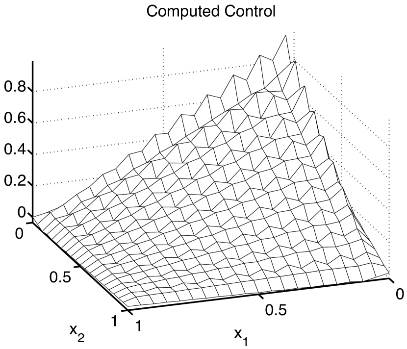
discretize-then-optimize

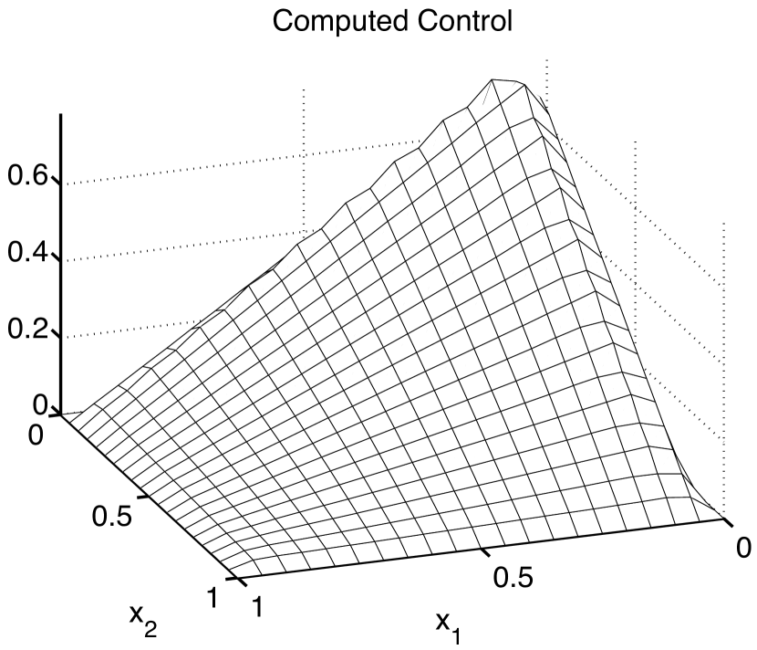
optimize-then-discretize

Figure 5.1: Computed controls, Example 3, $k=\ell=m=2$, $h=0.1$.

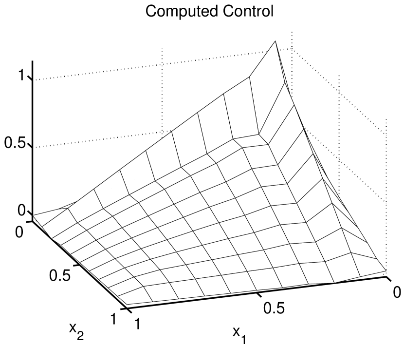
discretize-then-optimize

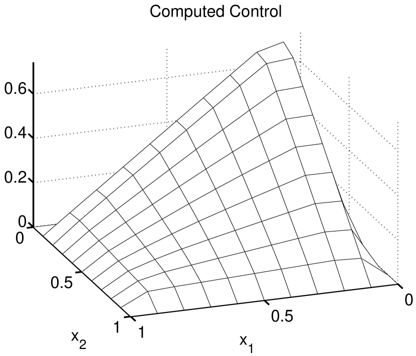
optimize-then-discretize

Figure 5.2: Computed controls, Example 3, $k=\ell=m=1$, $h=0.1$.

The observations drawn from Tables 5.5 and 5.6 for this example are very similar to those of Example 1. However, when quadratic finite elements are used, we observed small node-to-node oscillations in the adjoints and controls computed by the discretize-then optimize approach. These are not present in the adjoints and controls computed by the optimize-then-discretize approach. See Figure 5.1. Such node-to-node oscillations in the adjoints and controls did not develop in either approach when linear finite elements are used as seen in Figure 5.2. For better visibility we show the results on a coarse grid, but the plots of our results on finer grid are qualitatively comparable to those in Figures 5.1 and 5.2.

We remark that for this example the standard Galerkin method produced poor results. For smaller diffusion $\epsilon$ even SUPG using either approach did not produce satisfactory approximations to the optimal control, states and adjoints for coarser grids.

Table 5.5: Errors and estimated convergence order. Example 3, $k=\ell=m=1$.

The discretize-then-optimize approach

	$\|y_{h}-y_{\rm ex}\|$				$\|u_{h}-u_{\rm ex}\|$		$\|\lambda_{h}-\lambda_{\rm ex}\|$
$h$	$\|\cdot\|_{0}$	order	$\|\cdot\|_{SD}$	order	$\|\cdot\|_{0}$	order	$\|\cdot\|_{0}$	order	$\|\cdot\|_{SD}$	order
1.00e-1	1.20e-1		1.25e+0		4.91e-2		1.09e-1		1.26e+0
5.00e-2	7.43e-2	0.69	1.11e+0	0.17	2.48e-2	0.98	6.31e-2	0.79	1.09e+0	0.20
2.50e-2	4.17e-2	0.83	7.58e-1	0.55	1.36e-2	0.87	3.28e-2	0.94	7.22e-1	0.60
1.25e-2	1.46e-2	1.51	3.83e-1	0.99	5.88e-3	1.21	1.13e-2	1.54	3.69e-1	0.97
6.25e-3	3.86e-3	1.92	1.83e-1	1.07	1.68e-3	1.81	2.99e-3	1.92	1.81e-1	1.03

The optimize-then-discretize approach

	$\|y_{h}-y_{\rm ex}\|$				$\|u_{h}-u_{\rm ex}\|$		$\|\lambda_{h}-\lambda_{\rm ex}\|$
$h$	$\|\cdot\|_{0}$	order	$\|\cdot\|_{SD}$	order	$\|\cdot\|_{0}$	order	$\|\cdot\|_{0}$	order	$\|\cdot\|_{SD}$	order
1.00e-1	1.22e-1		1.25e+0		1.18e-1		1.18e-1		1.25e+0
5.00e-2	7.54e-2	0.70	1.11e+0	0.17	7.36e-2	0.69	7.36e-2	0.69	1.11e+0	0.17
2.50e-2	4.22e-2	0.84	7.59e-1	0.55	4.12e-2	0.83	4.12e-2	0.83	7.56e-1	0.55
1.25e-2	1.47e-2	1.52	3.83e-1	0.99	1.45e-2	1.51	1.45e-2	1.51	3.82e-1	0.98
6.25e-3	3.88e-3	1.92	1.83e-1	1.07	3.82e-3	1.92	3.82e-3	1.92	1.83e-1	1.06

Table 5.6: Errors and estimated convergence order. Example 3, $k=\ell=m=2$.

The discretize-then-optimize approach

	$\|y_{h}-y_{\rm ex}\|$				$\|u_{h}-u_{\rm ex}\|$		$\|\lambda_{h}-\lambda_{\rm ex}\|$
$h$	$\|\cdot\|_{0}$	order	$\|\cdot\|_{SD}$	order	$\|\cdot\|_{0}$	order	$\|\cdot\|_{0}$	order	$\|\cdot\|_{SD}$	order
2.00e-1	1.13e-1		6.56e-1		4.19e-2		1.09e-1		7.64e-1
1.00e-1	6.07e-2	0.89	9.12e-1	-0.48	1.60e-2	1.39	5.96e-2	0.87	9.50e-1	-0.31
5.00e-2	2.73e-2	1.15	7.56e-1	0.27	1.29e-2	0.31	3.60e-2	0.73	1.04e+0	-0.13
2.50e-2	5.42e-3	2.33	2.92e-1	1.37	6.53e-3	0.98	1.47e-2	1.29	7.05e-1	0.56
1.25e-2	6.35e-4	3.09	8.09e-2	1.85	2.16e-3	1.60	4.29e-3	1.78	3.96e-1	0.83

The optimize-then-discretize approach

	$\|y_{h}-y_{\rm ex}\|$				$\|u_{h}-u_{\rm ex}\|$		$\|\lambda_{h}-\lambda_{\rm ex}\|$
$h$	$\|\cdot\|_{0}$	order	$\|\cdot\|_{SD}$	order	$\|\cdot\|_{0}$	order	$\|\cdot\|_{0}$	order	$\|\cdot\|_{SD}$	order
2.00e-1	1.14e-1		6.54e-1		1.13e-1		1.13e-1		6.78e-1
1.00e-1	6.13e-2	0.90	9.14e-1	-0.48	6.05e-2	0.90	6.05e-2	0.90	9.07e-1	-0.42
5.00e-2	2.76e-2	1.15	7.57e-1	0.27	2.72e-2	1.15	2.72e-2	1.15	7.54e-1	0.27
2.50e-2	5.43e-3	2.34	2.92e-1	1.38	5.42e-3	2.33	5.42e-3	2.33	2.92e-1	1.37
1.25e-2	6.35e-4	3.10	8.09e-2	1.85	6.35e-4	3.09	6.35e-4	3.09	8.09e-2	1.85

6 Conclusions

We have studied the effect of the SUPG finite element method on the discretization of optimal control problems governed by the linear advection-diffusion equation. Two approaches for the computation of approximate controls and corresponding states and adjoints were compared: The discretize-then-optimize approach and the optimize-then-discretize approach. Theoretical and numerical studies of the error between the exact solution of the control problem and its approximation were provided. Our theoretical results show that the optimize-then-discretize approach leads to asymptotically better approximate solutions than the discretize-then-optimize approach. The theoretical results also indicate that the differences in solution quality is small when piecewise linear polynomials are used for the discretization of states, adjoints and controls, but that they can be significant if higher-order finite elements are used for the states and the adjoints. There is always a significant difference in quality of the adjoints computed by the discretize-then-optimize approach and the optimize-then-discretize approach if finite element approximations with polynomial degree greater than one are used, and the optimize-then-discretize approach leads to better adjoint approximations. However, our numerical results have also shown that this large difference in the quality of adjoints does not necessarily imply a large difference in the quality of the controls.

Often the observed error in the controls computed by the discretize-then-optimize approach and the optimize-then-discretize approach is rather similar – even if the adjoints computed using both approaches are significantly different. This seems to be related to the fact that we consider distributed controls and that errors in the controls are measured in the $L^{2}$ norm whereas errors in the adjoints are measured in the SUPG-norm. Since the distributed controls are multiples of the adjoints, our numerical results indicate that the $L^{2}$-error in the adjoints is much smaller than the error in the SUPG-norm. Whether these good convergence properties in the control also materialize if Neumann or Dirichlet boundary controls are used or if other objective functionals acting on the state are given is part of future studies. Another subject of future study is the influence of stabilization methods on the control of systems of advection diffusion equations, like the Navier-Stokes equations, where additional inconsistencies in the discretize-then-optimize approach can occur.

We conclude by reiterating that care is required when using the SUPG method for the solution of optimal control problems. If the discretize-then-optimize approach with SUPG is used, the order with which the computed solutions of the optimal control converge to the exact solution may be much lower than what one would expect from the solution of a single advection diffusion equation using SUPG. The asymptotic convergence behavior expected from the SUPG method applied to a single advection diffusion equation can be maintained for the optimal control problem if the optimize-then-discretize approach is used.

References

- [1] F. Brezzi and M. Fortin, Mixed and Hybrid Finite Element Methods, Computational Mathematics, Vol. 15, Springer–Verlag, Berlin, 1991.
- [2] A. N. Brooks and T. J. R. Hughes, Streamline upwind/Petrov–Galerkin formulations for convection dominated flows with particular emphasis on the incompressible Navier–Stokes equations, Comp. Meth. Appl. Mech. Engng., 32 (1982), pp. 199–259.
- [3] P. G. Ciarlet, Basic error estimates for elliptic problems, in Handbook of Numerical Analysis, Vol.2: Finite Element Methods (Part 1), P. Ciarlet and J. Lions, eds., Elsevier/North–Holland, Amsterdam, New York, Oxford, Tokyo, 1991.
- [4] L. P. Franca, S. L. Frey, and T. J. R. Hughes, Stabilized finite element methods. I. Application to the advecive diffusive model, Comp. Meth. Appl. Mech. Engng., 95 (1992), pp. 253–276.
- [5] P. Grisvard, Elliptic Problems in Nonsmooth Domains, Pitman, Boston, London, Melbourne, 1985.
- [6] T. J. R. Hughes, L. P. Franca, and G. M. Hulbert, A new finite element formulation for computational fluid dynamics. VIII. the Galerkin/least squares methods for advecive–diffusive systems, Comp. Meth. Appl. Mech. Engng., 73 (1989), pp. 173–189.
- [7] K. Jansen, S. S. Collis, C. Whiting, and F. Shakib, A better consistency for low-order stabilized finite element methods, Comput. Methods Appl. Mech. Engrg., 174 (1999), pp. 153–170.
- [8] C. Johnson, U. Nävert, and J. Pitkäranta, Finite element methods for linear hyperbolic problems, Comp. Meth. Appl. Mech. Engng., 45 (1984), pp. 285–312.
- [9] P. Knabner and L. Angermann, Numerik partieller Differentialgleichungen, Springer–Verlag, Berlin, Heidelberg, New York, 2000.
- [10] J. L. Lions, Optimal Control of Systems Governed by Partial Differential Equations, Springer Verlag, Berlin, Heidelberg, New York, 1971.
- [11] K. W. Morton, Numerical Solution of Convection–Diffusion Problems, Chapman & Hall, London, Glasgow, New York, 1996.
- [12] A. Quarteroni and A. Valli, Numerical Approximation of Partial Differential Equations, Springer, Berlin, Heidelberg, New York, 1994.
- [13] H. G. Roos, M. Stynes, and L. Tobiska, Numerical Methods for Singularly Perturbed Differential Equations, Computational Mathematics, Vol. 24, Springer–Verlag, Berlin, 1996.
- [14] G. Zhou, How accurate is the streamline diffusion finite element method?, Math. Comp., 66 (1997), pp. 31–44.
- [15] G. Zhou and R. Rannacher, Pointwise superconvergence of the streamline diffusion finite-element method, Numer. Methods Partial Differential Equations, 12 (1996), pp. 123–145.