Learning Parameter Sharing with
Tensor Decompositions and Sparsity

Abstract

Large neural networks achieve remarkable performance, but their size hinders deployment on resource-constrained devices. While various compression techniques exist, parameter sharing remains relatively unexplored. This paper introduces Fine-grained Parameter Sharing (FiPS), a novel algorithm that leverages the relationship between parameter sharing, tensor decomposition, and sparsity to efficiently compress large vision transformer models. FiPS employs a shared base and sparse factors to represent shared neurons across multi-layer perception (MLP) modules. Shared parameterization is initialized via Singular Value Decomposition (SVD) and optimized by minimizing block-wise reconstruction error. Experiments demonstrate that FiPS compresses DeiT-B and Swin-L MLPs to 25–40% of their original parameter count while maintaining accuracy within 1 percentage point of the original models.

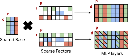
Figure 1: FiPS.

1 Introduction

Over the last decade, large neural networks have achieved impressive performance across various tasks by scaling up datasets and model sizes. However, this growth has led to computational, memory, and storage challenges, necessitating efficient model compression techniques to reduce overhead and enable deployment on resource-constrained devices like mobile phones and embedded systems. To this end, research has explored various approaches, including tensor decomposition, quantization, distillation, sparsity, parameter sharing, and adaptive computing methods (Cheng et al., 2020). While most of these methods are well-studied and successfully utilized in practice (e.g., distillation, quantization), parameter sharing has received less attention.

Sharing parameters across multiple layers of a neural network could, in theory, reduce memory requirements and increase cache hits, leading to faster execution. Motivated by this, several previous works have explored reusing entire transformer blocks when defining a network (Lan et al., 2020; Takase & Kiyono, 2023; Lin et al., 2023), resulting in more efficient models. Although the ability to share weights unmodified across layers is promising, we hypothesize that a more fine-grained approach may achieve better compression, leading us to focus on sharing neurons across different layers.

We show that sharing neurons across layers can be achieved using a shared basis, where each neuron is computed as a linear combination of this basis. Crucially, we find that sparsity in the projection matrix is essential for this approach to be effective. This insight leads to our novel parameter sharing algorithm, Fine-grained Parameter Sharing (FiPS), which we demonstrate effectively compresses large vision transformer models. Our contributions include:

• We demonstrate that sharing neurons across multiple layers is feasible through sparse tensor decomposition.

• We explore various neuron-sharing alternatives, emphasizing the importance of selecting appropriate bases and sparse factors for enhanced compression.

• Building on these findings, we introduce FiPS, which utilizes Singular Value Decomposition (SVD) for initialization and optimizes decomposed parameters by minimizing block-wise reconstruction error.

• FiPS compresses the MLP modules of DeiT-B (Touvron et al., 2021) and SWIN-L (Liu et al., 2021) to 25–40% of their original size while maintaining minimal accuracy loss (less than 1 percentage point).

2 Parameter Sharing Through Sparse Tensor Decomposition

Consider a weight matrix, $\mathbf{W}\in\mathbb{R}^{d\times p}$, which projects feature vectors from $d$-dimensional space to a $p$-dimensional space, with neurons represented as the columns of $\mathbf{W}$. We aim to share weights across a subset of these $p$ neurons such that there remain only $r<p$ unique neurons; in other words, we want only $r$ columns of $\mathbf{W}$ to have unique values. We can represent the $r$ unique neurons using a lookup table (basis matrix) $\mathbf{U}\in\mathbb{R}^{d\times r}$. Then, our original matrix $\mathbf{W}$ can be reconstructed using an $r$-dimensional one-hot vector for each of its $p$ columns, represented by a projection matrix $\mathbf{V}\in\mathbb{R}^{r\times p}$. This is the "one-hot" approach illustrated in the upper part of Figure 1. Note that the number of unique neurons in this setting is $r$, which limits the representation power of the resulting matrix $\mathbf{W}$. One way to alleviate this limitation is to increase the number of non-zero elements in $\mathbf{V}$, effectively creating combinations of the basis neurons and resulting in significantly more unique neuron representations, as illustrated in the lower part of Figure 1. So far, we have considered sharing neurons within a single matrix $\mathbf{W}$. However, this approach can be easily extended to multiple weight matrices $\mathbf{W}_{1},\ldots,\mathbf{W}_{N}$. Specifically, we can enable fine-grained parameter sharing across multiple layers by increasing the size of our projection matrix $\mathbf{V}$ and shared basis $\mathbf{U}$.

The approach outlined above can be viewed as a low-rank decomposition of a matrix $\mathbf{W}$, where the first factor $\mathbf{U}$ is shared and the second factor $\mathbf{V}$ is sparse. Thus, we can utilize existing low-rank decomposition techniques to obtain an optimal shared orthogonal basis and induce sparsity in the projection matrices using existing pruning and sparse training techniques. In what follows, we use a pre-trained DeiT-B model (with 12 encoder blocks, each containing one MLP modules, pre-trained on ImageNet-1k (Deng et al., 2009)) and investigate the best strategy for tying multiple layers using the described framework. Specifically, we focus on the model’s MLP modules, each consisting of two fully-connected (FC) layers with dimensions $\mathbb{R}^{d\times p}$ and $\mathbb{R}^{p\times d}$ respectively, where $p=4d$.

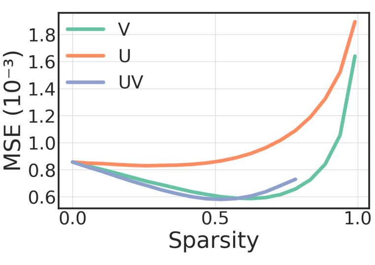
(a) Optimal Sparsity: FC-1

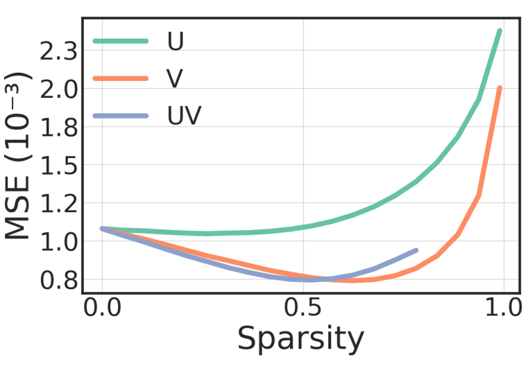
(b) Optimal Sparsity: FC-2

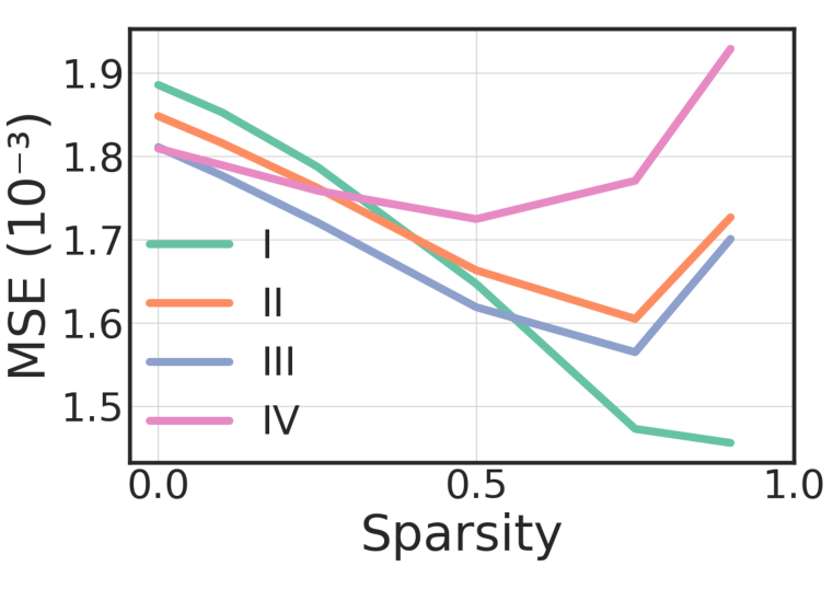
(c) Parameter Sharing Strategies.

Figure 2: Initial Experiments. Reconstruction error when inducing sparsity on different factors of low-rank decomposition of (2(a)) the FC-1 layer and (2(b)) the FC-2 layer, under a parameter budget of 25%. Higher sparsities, when applied to larger factors, enable higher ranks and achieve lower error. (2(c)) Average reconstruction error of four FC layers under different parameter sharing strategies and sparsities. See § 2.2 for a description of each strategy.

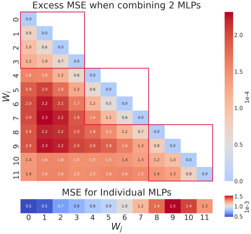
(a) Mean-Squared Error (MSE) compressing MLP module pairs of diff. blocks.

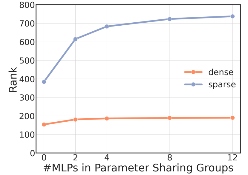
(b) Rank.

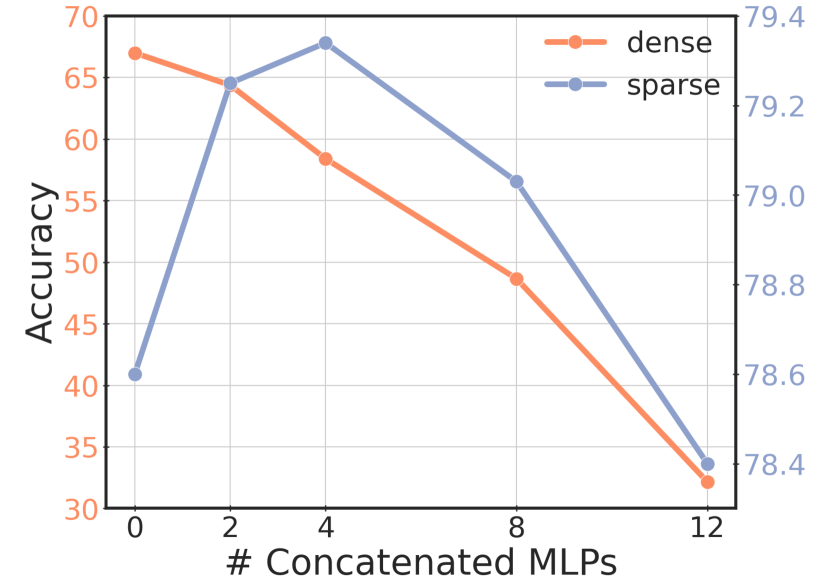
(c) Accuracy.

Figure 3: Parameter Sharing Groups. (3(a) top) Increase in mean squared error (MSE) when sharing $\mathbf{U}$ between different MLP modules, (3(a) bottom) MSE when compressing individual MLP modules. Sharing $\mathbf{U}$ among consecutive layers often achieves the smallest error. (3(b)) With a fixed parameter budget, the rank of the shared basis $\mathbf{U}$ plateaus around four MLP modules (3(c)) aligning with the optimal group size for maximizing accuracy when compressing the DeiT-B model using our algorithm.

2.1 Optimal Sparsity for Tensor Decomposition

Before moving on to parameter sharing through shared bases, we decompose individual FC layers using a truncated SVD with a 25% parameter budget and introduce sparsity by setting low-magnitude values to zero. We consider introducing sparsity in: (1) $\mathbf{U}$, (2) $\mathbf{V}$, and (3) both $\mathbf{U}$ and $\mathbf{V}$. We vary the sparsity of matrices while keeping the total number of non-zero parameters fixed. The resulting reconstruction errors are shown in Figures 2(a) and 2(b). We observe that the best errors are achieved around 60–80% sparsity and when sparsity is introduced on the larger factor (i.e., $\mathbf{V}$). We believe this is because larger matrices have more redundant weights and, thus, easier to prune.

2.2 Weight Concatenation and Finding Shared Dimensions

Next, we study introducing parameter sharing across multiple layers within a network. Specifically, we consider four FC layers from two different MLP modules and concatenate their parameters in different ways to find the optimal strategy for constructing the shared basis.

First, we transpose the parameters of the second FC layers in each MLP module, such that each layer is represented by a weight matrix $\mathbf{W}\in\mathbb{R}^{d\times 4d}$. We then explore four distinct ways of concatenating 2 MLP modules together (four FC layers in total):

1. Concatenate all matrices along the longer axis: $\mathbf{W_{s}}\in\mathbb{R}^{d\times 16d}$.

2. Concatenate FC layers from the same module along the longer axis and then different modules along the shorter: $\mathbf{W_{s}}\in\mathbb{R}^{2d\times 8d}$.

3. Concatenate FC layers from the same module along the shorter axis and then different modules along the longer: $\mathbf{W_{s}}\in\mathbb{R}^{2d\times 8d}$.

4. Concatenate all layers along the shorter axis: $\mathbf{W_{s}}\in\mathbb{R}^{4d\times 4d}$.

We apply truncated SVD to the concatenated matrix $\mathbf{W_{s}}$, and keep the top $r$ singular vectors. The resulting matrix $\mathbf{V}$ (corresponding to the right singular vectors) is sparsified by keeping the entries with the largest magnitude, an approach shown in § 2.1 to yield optimal reconstruction. Finally, we reconstruct the parameters using a shared basis and report the mean squared error (MSE) in Figure 2(c). Concatenating weights along the longer dimension yields the best reconstruction error, especially at higher sparsity levels. Therefore, going forward, we will always concatenate the two FC layers of every MLP module in the transformer blocks along their larger dimension.

2.3 Parameter Sharing Across Layers

In this section, we study the redundancy and interplay among different MLP modules to identify ideal groups for parameter sharing. First, we decompose individual modules using a rank of $r=180$ and plot the MSE in Figure 3(a)-bottom. We observe that the error increases almost monotonically with the module index, suggesting the need for allocating more capacity to later modules in the network.

Next, we group two MLP modules from two blocks ($i$ and $j$) and make them share the same basis $\mathbf{U}$, which reduces the parameter count and consequently increases the MSE for each block. The MSE for block $i$ in this shared setting is denoted as $MSE_{i,j}$. In Figure 3(a), we plot the average MSE increase between blocks $i$ and $j$ as $MSE^{\uparrow}_{i,j}=(MSE_{i}-MSE_{i,j}+MSE_{j}-MSE_{j,i})/2$. Empirically, we find that nearby blocks tend to have the smallest increase in error, motivating the grouping of consecutive layers when sharing parameters.

We then study the optimal number of MLP modules per group. Increasing the group size, thereby sharing more parameters across the same basis $\mathbf{U}$, allows for a higher rank, as shown in Figure 3(b). This effect is more pronounced when sparsity is applied to factor $\mathbf{V}$. However, a higher rank does not always lead to better accuracy, as the shared basis must cover a larger number of parameters. As illustrated in Figure 3(c), the highest post-compression accuracy is attained when parameters are shared across the MLP modules four consecutive blocks.

3 Sparsity-enabled Parameter Sharing

Experiments in the previous section motivate and guide us in developing FiPS, an efficient parameter-sharing algorithm enabled by sparse tensor decompositions that can be summarized in three main points:

1. Shared Initialization: We tie multiple fully connected layers across a group of MLP modules and apply low-rank decomposition via truncated SVD.

2. Local Error Minimization: We finetune our shared low-rank initialization to minimize the difference between the activations of the original and compressed model. During this step, we also introduce sparsity in our factors, which helps us allocate parameters where they are most needed.

3. Global Error Minimization (Optional): For best results, especially at lower compression levels, we finetune our compressed models end-to-end.

Algorithm 1 outlines the key steps of FiPS, which are detailed below.

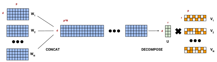
Figure 4: Parameter Sharing Through Sparse Tensor Decomposition. A group of FC layers are concatenated along the larger dimension, $p$, and decomposed into two matrices: a shared basis, U, and a sparse projection matrix, which is then sliced up respectively for each layer.

Shared Initialization.

We begin by compressing the pre-trained model through parameter sharing, achieved by concatenating and decomposing multiple FC layers simultaneously, as illustrated in Figure 4. For higher parameter budgets and sparsity levels (e.g., 50% and 75%, respectively), the rank of our low-rank factor $\mathbf{U}$ can exceed the model dimension $d$. In such cases, we grow the matrices $\mathbf{U}$ and $\mathbf{V}$ similar to the approach in Net2Net (Chen et al., 2016). However, unlike Net2Net, we grow $\mathbf{U}$ by appending zeros rather than splitting each neuron. We select the top-$k$ neurons with the highest singular values (i.e., $k=r-d$) and multiply them by $\nicefrac{{1}}{{\tau}}$, where $\tau$ is treated as a hyperparameter (discussed further in § 5).

Formally, the parameters of a group of FC layers, $\mathbf{W}_{1},\mathbf{W}_{2},\dots,\mathbf{W}_{N}$, are concatenated into a large matrix $\mathbf{W_{s}}=[\mathbf{W}_{1};\mathbf{W}_{2};\dots;\mathbf{W}_{N}]$, where $\mathbf{W}_{i}\in\mathbb{R}^{d\times p}$ . We then apply truncated SVD, $\mathbf{W_{s}}=\mathbf{U}\mathbf{\Sigma}\mathbf{\hat{V}}$, to obtain a low-rank approximation of the parameters, where $\mathbf{U}\in\mathbb{R}^{d\times r}$, $\mathbf{\Sigma}\in\mathbb{R}^{r\times r}$, and $\mathbf{\hat{V}}\in\mathbb{R}^{r\times(N\cdot p)}$. The factor $\mathbf{U}$ is shared among all layers within the group and remains dense due to its relatively small size. Next, we multiply $\mathbf{\hat{V}}$ by the singular values to obtain the projection matrix $\mathbf{V}=\mathbf{\Sigma}\mathbf{\hat{V}}$. Finally, the weights are reconstructed as $\mathbf{W^{\prime}}_{i}=\mathbf{U}\mathbf{V}_{i}$, where each $\mathbf{V}_{i}$ is a slice of $\mathbf{V}$ corresponding to the weight matrix $\mathbf{W}_{i}$.

Local Error Minimization

For the second phase of our method, we compute the input and output activations of the original FC layers using a calibration dataset $D$, described in § 4. We use these activations to optimize the compressed layers and minimize the L2-loss between the original and compressed layers’ activations:

$$\operatorname*{argmin}_{\mathbf{U,V_{i},\dots,V_{N}}}\sum_{i}^{N}{\|\mathbf{W}_{i}\mathbf{X}_{i}-\mathbf{U}\mathbf{V}_{i}\mathbf{X}_{i}\|_{2}^{2}},$$ (1)

where $\mathbf{X}_{i}$ is the inputs to the $i^{\textrm{th}}$ original FC layer. We explore several sparse training and pruning techniques to identify a sparse $\mathbf{V}$ during this optimization: (a) Static Sparsity, which establishes the sparsity structure by retaining the top-magnitude connections before training (Hoefler et al., 2021); (b) Gradual Magnitude Pruning (GMP) (Zhu & Gupta, 2017), which progressively increases sparsity by updating its mask every $T$ steps, retaining the top-magnitude connections following the cubic schedule from Kurtic et al. (2023); and (c) RigL (Evci et al., 2021), which starts from (a) but updates the sparse connectivity every $\Delta T$ steps using gradient and magnitude information. We decided to use GMP for the final sparse training recipe due to its superior performance.

Although we share parameters across multiple MLP modules, gradients for error minimization can be computed one MLP module at a time. Therefore, optimization requires significantly fewer resources compared to end-to-end fine-tuning.

Global Error Minimization.

In this optional stage, we finetune the shared parameterization found in the previous stage end-to-end to further improve our results. Because our factors $\mathbf{V}_{i}$ are sparse, we employ the dynamic sparse training method, RigL, during this stage as we observe it to perform slightly better than keeping the sparsity pattern constant (i.e., Static Sparsity) as discussed in § 4.

Memory and Latency

Let’s assume we are applying FiPS to compress a matrix $\mathbf{W}\in\mathbb{R}^{d\times p}$ to a fraction $F\in[0,1]$ of its original size while having a fraction $D\in[0,1]$ of non-zero parameters in the resulting factors. Then, using the equality $Fdp=Dr(d+p)$, we can calculate the required rank, $r=\nicefrac{{Fdp}}{{D(d+p)}}$. The cost of storing a sparse matrix depends on the storage format. Here, we assume a bitmask for simplicity, where non-zero values are indicated with 1s. Assuming parameters are represented with 16 bits, the storage cost can be calculated as the sum of parameter and mask bits: Substituting r and dividing by the cost of storing the original matrix (i.e., $16dp$), we can calculate storage savings as follows: $F_{sparse}=\nicefrac{{17F}}{{16D}}$. This equality indicates that, to achieve storage savings, we need to increase sparsity roughly at the same rate as the overall compression rate, requiring $\nicefrac{{F}}{{D}}<0.94$.

Next, we consider the multiply-add-operations (MACs) required for compressed layers, which can be implemented following one of the two strategies:

1. Low rank: We can perform (potentially) low rank matrix computation, i.e. $\mathbf{Y}=(\mathbf{X}\mathbf{U})\mathbf{V}$, which requires MACs proportional to the compression factor $F$.

2. Full rank: We can materialize the matrix $\mathbf{W}=\mathbf{U}\mathbf{V}$ first and then perform the regular matrix computation. This would cost at least as much as the original matrix multiplication plus the materialization cost. However, if the matrix is used multiple times (i.e. if the batch size is much larger than the rank), then the materialization cost can be amortized. Although the number of MACs is not reduced, this strategy could lead to faster runtime due to reduced memory transfer and communication. Thus, it could be beneficial in distributed or federated learning settings.

Algorithm 1 Fine-grained Parameter Sharing

1:MLP parameters $\mathbf{W}_{1},\cdots,\mathbf{W}_{N}\in\mathbb{R}^{d\times p}$, MLP inputs $\mathbf{A}_{i}$ and MLP function $\mathbf{f}(\mathbf{W}_{i},\ \mathbf{A}_{i})$, Target rank $r$, Learning Rate $\mathbf{\eta}$, Steps $\mathbf{T}$.

2:$\mathbf{U},\ \left[\mathbf{V}_{1},\mathbf{V}_{2},\cdots,\mathbf{V}_{N}\right]\leftarrow\mathit{TruncatedSVD}\left(\left[\mathbf{W}_{1};\mathbf{W}_{2};\cdots;\mathbf{W}_{N}\right],\ k=r\right)$

3:for each training iteration $t=1$ to $T$ do

4:     $\mathbf{G_{U}}=0$ $\triangleright$ Gradient accumulator for $\mathbf{U}$

5:     for each block $i$ do

6:         $\mathbf{V}_{i}\leftarrow\mathit{Sparsify}(\mathbf{V}_{i},\ t)$ $\triangleright$ Potentially increase or adjust sparsity

7:         $L_{i}\leftarrow\mathit{MSE\_loss}(\mathbf{f}(\mathbf{W}_{i},\ \mathbf{A}_{i}),\quad\mathbf{f}(\mathbf{U}\,\mathbf{V_{i}},\ \mathbf{A}_{i}))$

8:         $\mathbf{V}_{i}\leftarrow\mathbf{V}_{i}-\eta\nabla_{\mathbf{V}_{i}}L_{i}$

9:         $\mathbf{G_{U}}\leftarrow\mathbf{G_{U}}+\mathbf{\nabla_{U}}L_{i}$

10:     end for

11:     $\mathbf{U}\leftarrow\mathbf{U}-\dfrac{\eta}{N}\mathbf{G_{U}}$

12:end for

13:return $\mathbf{U},\ [\mathbf{V}_{1},\ldots,\mathbf{V}_{N}]$

4 Main Results

Experimental Setup

In our experiments, we used DeiT-B (with 12 blocks) and Swin-L (four stages containing $2$, $2$, $18$, and $2$ blocks, respectively) (Touvron et al., 2021; Liu et al., 2021). We used a calibration dataset $D$ of $30\times 128=3840$ samples from ImageNet-1k (Deng et al., 2009). We found that 20 epochs with this calibration set yielded near-optimal results, while longer training or larger calibration sets yielded marginal improvements. This calibration stage took <1 hour on an Nvidia A6000 GPU for both architectures. Transfer learning capability was assessed on CIFAR-100, Flowers102, Oxford-III-Pets, and iNaturalist 2019 datasets (Krizhevsky, 2009; Nilsback & Zisserman, 2008; Parkhi et al., 2012; Van Horn et al., 2018) using 100 training epochs, following the methodology of Yu & Wu (2023). In all our experiments, we used AdamW optimizer (Loshchilov & Hutter, 2019) and identified the optimal learning rates by performing a small hyperparameter sweep using $12$ logarithmically spaced values.

When applying FiPS, we targeted 75% average sparsity across all sparse factors, as this resulted in the best compression, as shown in Figure 5(b). The mask update interval, $\Delta T$, for both RigL and GMP was set to 50 steps. When using RigL during global fine-tuning, we used an initial pruning ratio of $0.1$ and reduced this value to $0.05$ during our transfer learning experiments to limit changes in the sparsity pattern. Further hyperparameter details for the optimizer and the sparse training algorithms used are provided in § A.2.

Following our earlier results (i.e., Figure 3(c)), we used groups of four consecutive blocks (each with one MLP module) for the DeiT-B architecture, resulting in three different parameter-sharing groups. For Swin, we shared parameters within each 2-block stage separately and split the remaining stage with 18 blocks into three groups with six consecutive blocks each.

ImageNet-1k

We compare FiPS against the baselines of Adaptive Atomic Feature Mimicking (AAFM), which utilizes block-wise error minimization, and Global Feature Mimicking (GFM), combining AAFM with distillation at the model output, both of which are proposed by Yu & Wu (2023).

Table 1: Compressing Models Pretrained on ImageNet-1k. We compare top-1 val. accuracy (%) of DeiT-B (81.85%) (Touvron et al., 2021) and Swin-L (86.24%) (Liu et al., 2021) models compressed using FiPS vs. AAFM/GFM across parameter budgets. Results include layer-wise error minimization (FiPS) and global error minimization (FiPS + FT). AAFM/GFM^† results are from Yu & Wu (2023).

Param. Budget	10%		25%		40%		50%		75%
Method / Model	DeiT	Swin	DeiT	Swin	DeiT	Swin	DeiT	Swin	DeiT	Swin
AAFM †	–	–	–	–	80.33	–	81.21	85.04	–	–
GFM †	–	–	–	–	81.28	–	81.62	85.33	–	–
FiPS (ours)	70.04	74.04	80.64	84.78	81.69	85.69	81.83	85.99	81.82	86.21
FiPS + FT (ours)	77.26	82.13	81.31	85.16	81.55	85.68	81.54	85.99	–	–

At a 40% parameter budget, FiPS achieves 1.36% point higher accuracy (shown in Table 1) than AAFM and even exceeds the costly GFM approach by 0.41% point, which requires significantly higher memory and computing resources due to the need for end-to-end fine-tuning.

As for Swin-L, the picture is similar as shown in Table 1. Across all parameter budgets, GMP-based FiPS consistently achieves higher accuracies than alternatives like GFM while requiring less computing and memory to compress the pre-trained model.

Transfer Learning

Table 2: Transfer Learning Results. We compare the top-1 accuracy of the original DeiT-B model with compressed versions using GFM and FiPS across various MLP parameter budgets on small-scale datasets. GFM^† and Original^† results are from Yu & Wu (2023) and Touvron et al. (2021), respectively.

Models	Original†	GFM†		FiPS +RigL FT (ours)
Param. Budget	100%	40%	50%	25%	40%	50%
CIFAR-100	90.99	90.17	90.67	90.88	91.24	91.33
Pets	94.74	93.95	94.22	94.19	94.52	94.41
Flowers102	97.77	97.02	97.45	97.84	98.14	98.37
iNaturalist-2019	77.39	77.13	77.56	77.26	77.58	77.69

Next, we take our compressed models and finetune them on four different transfer tasks. Since the factors are already sparse, we use RigL to adapt the sparse factors. Models compressed through FiPS result in significantly better transfer accuracies as shown on Table 2.

5 Ablations

In this section, we study the importance of various components of the FiPS algorithm when compressing the DeiT-B model at different parameter budgets. First, we ablate key components of our algorithm in Figure 5(a) under a 25% parameter budget:

1. SVD-based Initialization: Using a random initialization (RI) instead of SVD-based initialization results in a 1% point drop in accuracy.

2. Global Pruning: We use global pruning (GP) when sparsifying our sparse factors $\mathbf{V}$, which results in 0.4% point improvement over local pruning (LP), which enforces the same sparsity level for each factor $\mathbf{V}_{i}$.

3. Scaling Vectors: We normalize the weight matrix $\mathbf{W}$ before the initial SVD stage of FiPS as suggested by Liu et al. (2024). While normalized weights are used during our SVD based initialization, magnitude vectors are used to initialize new scaling vectors (SV), used in scaling individual neurons. Although incorporating scaling vectors improves over local pruning, it is less effective when combined with global pruning.

Consequently, the final FiPS configuration integrates GMP with GP. Next, we perform a sensitivity analysis using different sparsity levels, calibration dataset sizes, and training lengths using the DeiT-B checkpoint trained on ImageNet-1k.

Optimal Sparsity for Sparse Factors

We compressed the DeiT-B model, as described in § 4, using sparsity levels ranging from 50% to 96% at a reduced parameter budget of 17.5%, as shown in Figure 5(b). The best performance was observed at 75% sparsity as shown in Figure 5(b). While increasing sparsity to 87% yielded similar accuracy, lowering it to 50% resulted in a notable drop in performance, likely due to a significant reduction in rank.

Calibration Dataset Size and Training Length

We examine the relationship between the number of batches and the number of epochs using a fixed batch size of 128 and a 50% parameter budget. We require the calibration set to have at least 3 data points per category for generalization (i.e., 30 batches) and observe that increasing the number of calibration data points results in less than 0.1% point improvement. Similarly, training beyond 20 epochs often results in worse generalization.

Alternative Sparsity Techniques

In addition to GMP, we considered using Dense tensor decompositions (i.e., no sparsity on $\mathbf{V}$ factors) and other sparse training techniques: Static Sparsity and RigL. Results are presented in Table 3. In the case of DeiT-B, for parameter budgets from 10–50%, RigL consistently outperforms Dense and Static Sparsity. At higher budgets, all methods converge to nearly identical accuracies approaching the original model accuracy. For Swin-L, RigL outperforms Dense and Static Sparsity at 10% and 25% parameter budgets. However for higher parameter budgets, Static Sparsity obtains slightly higher accuracies.

Sparsity Distribution and MSE-loss

Figure 6(a) shows that earlier MLP layers are easier to compress, requiring fewer parameters, while later layers are more challenging, as reflected by higher reconstruction errors in Figure 3(a). These later layers exhibit lower sparsity and higher weight density, with Figure 6(b) highlighting a strong correlation ($0.922$) between weight density and MSE. This indicates that later layers demand more parameters to preserve performance.

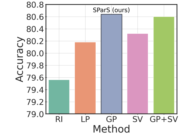
(a) Ablation Results.

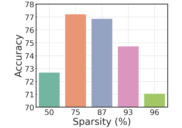
(b) Optimal Sparsity.

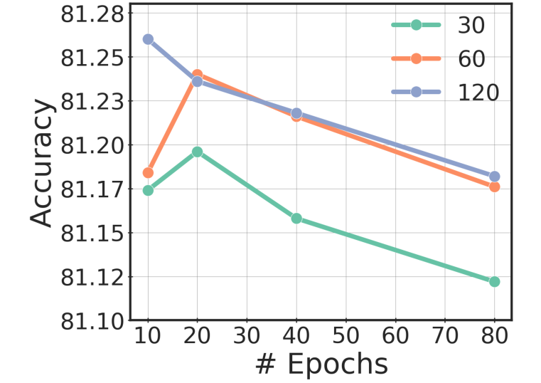
(c) Calibration Dataset Size.

Figure 5: Ablations and Sensitivity Analysis. ((5(a)) Ablation of key ingredients of the FiPS algorithm: random initialization (RI), Local Pruning (LP), Global Pruning (GP), and Scaling Vectors (SV); (5(b)) Effect of sparsity used in sparse factors; (5(c)) Effect of calibration dataset size (denoted as #batches with 128 images each) and # training epochs to post-compression accuracy.

Table 3: Sparsification Method and FiPS Generalization Performance. ImageNet top-1 validation accuracy (%) of DeiT-B (81.85%) (Touvron et al., 2021) and Swin-L (86.24%) (Liu et al., 2021) models compressed with FiPS using different sparsity methods: RigL (Evci et al., 2021) and static sparsity.

Param. Budget	10%		25%		40%		50%		75%
Method / Model	DeiT	Swin	DeiT	Swin	DeiT	Swin	DeiT	Swin	DeiT	Swin
Dense	15.35	3.61	65.71	60.31	74.33	80.61	79.22	83.59	81.36	85.64
Static Sparsity	65.26	65.6	80.06	84.37	81.48	85.69	81.70	85.98	81.86	86.23
RigL	66.67	70.96	80.31	84.57	81.50	85.59	81.65	85.91	81.82	86.20
GMP (FiPS)	70.04	74.04	80.64	84.78	81.69	85.69	81.83	85.99	81.82	86.21

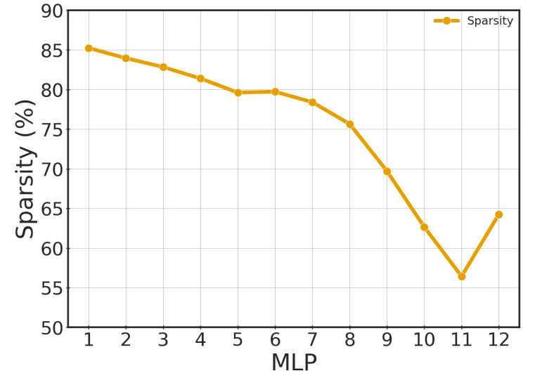
(a) Sparsity Distribution.

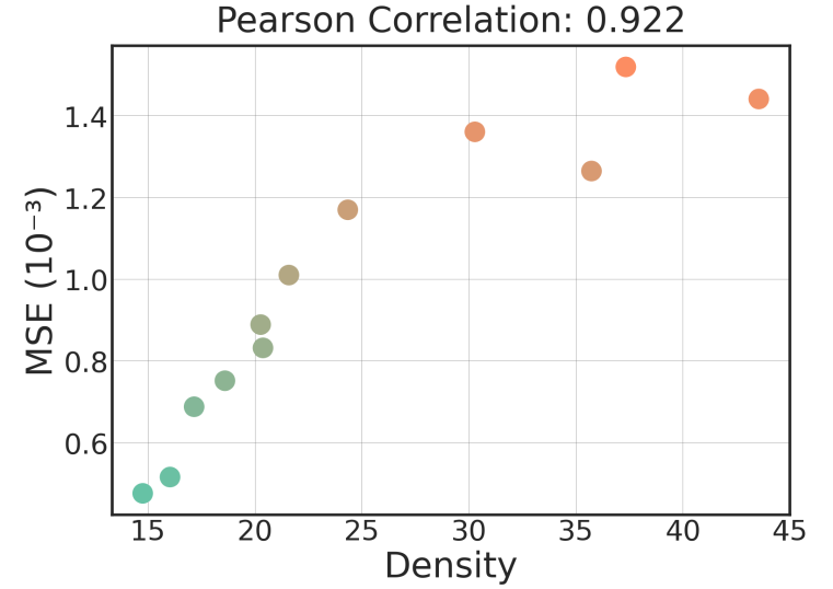
(b) Excess MSE vs. Weight Density.

Figure 6: Efectiveness of Global Sparsity. (6(a)) Average sparsity in the MLP modules of DeiT-B at the end of the training, showing more parameters are allocated to later modules. (6(b)) We observe a high correlation between the MSE values reported in Figure 3(a) and the parameter distribution found by FiPS.

Growing Neurons in the Shared Bases and Sparse Factors

As discussed in § 3, high parameter budgets and sparsity levels (e.g., 50% and 75%, respectively, for DeiT-B) often allow the rank $r$ to exceed the model dimension $d$. Note that the SVD used in our algorithm provides only d directions for initialization. We explore three methods for initializing the remaining $k=r-d$ dimensions: 1. Random Growth:New neurons in $\mathbf{U}$ are initialized to zero, and those in $\mathbf{V}$ are initialized randomly using He et al. (2015); 2. Neuron Splitting:The top $k$ neurons of $\mathbf{U}$ are duplicated, and the top $k$ neurons of $\mathbf{V}$ are halved to generate new neurons, similar to the method proposed by Chen et al. (2016). 3. Hybrid Initialization:New neurons in $\mathbf{U}$ are initialized to zero, while those in $\mathbf{V}$ are derived from the top $k$ neurons and normalized by a hyperparameter $\tau$. This zero initialization minimizes the immediate impact of the new neurons in $\mathbf{V}$, allowing the optimization process to gradually re-activate them during training, as suggested by Evci et al. (2022). After conducting a hyperparameter sweep on $\tau$, we found that the hybrid initialization approach outperformed the alternatives, obtaining accuracies 1% and 2% points higher than the alternatives (1) and (2), respectively.

6 Related Work

Vision Transformers (ViT) were introduced by Dosovitskiy et al. (2021) as a novel approach to image recognition by using image patches as sequences analogous to tokens in NLP models. DeiT (Data-efficient Image Transformer) introduced by Touvron et al. (2021) focuses on improving ViT’s data efficiency by using a specialized distillation token during training, which helps the model learn from a teacher network. Finally, Swin Transformer, proposed by Liu et al. (2021), differs from ViT and DeiT as it introduces a hierarchical structure and shifted windows for computing self-attention locally within non-overlapping windows.

Sparsity In Neural Networks can be grouped into three main approaches: sparsify post-training (i.e. pruning), sparsify during training, and fully sparse training (Hoefler et al., 2021). Various approaches have been explored for the pruning and sparsifying during training, starting with simple heuristic methods such as pruning the smallest magnitude parameters in a network (Thimm & Fiesler, 1995; Ström, 1997) to gradually increasing the amount of magnitude pruned parameters, namely GMP (Zhu & Gupta, 2017). Kurtic et al. (2023) extended this work by demonstrating the benefits of dynamic pruning with an accelerated cubic scheduler. Static sparsity is explained by Hoefler et al. (2021) as a simple, sparse training approach, where a mask initialized before training is used throughout. Hoefler et al. (2021) also examines the trade-offs between uniform pruning — where sparsity is applied equally across all layers — and global pruning, which distributes sparsity dynamically based on the importance of individual weights. Finally, the RigL algorithm (Evci et al., 2021), a dynamic sparse training method, adjusts the sparsity pattern during training by periodically pruning and regrowing connections based on gradient information.

Tensor Decomposition Aghajanyan et al. (2020) show that learned over-parameterized models reside in a low intrinsic dimension. The tensor decomposition approaches presented by Kolda & Bader (2009) are used in neural network compression to reduce redundancy of large weight matrices through applying low-rank decomposition. Yu & Wu (2023), for example, introduces AAFM for transformer-based models using a proxy dataset to compute the block activations and apply truncated PCA to reconstruct the weights. Additionally, they propose GFM to minimize the loss between the compressed model and the original model outputs, similar to teacher-student model training in Knowledge Distillation techniques (Hinton et al., 2015).

Parameter Sharing is perhaps the least explored area among the other compression areas cited above. Eban et al. (2019) use a $2M$ Sum-Product reducer to introduce structured hashing to map shared parameters model layers. Obukhov et al. (2021) utilizes TR decomposition to create shared parameters between 3D tensors. Moreover, Zhang et al. (2022) introduces “Weight Multiplexing”, corresponding to using shared parameters between MLP modules of ViT and doing distillation. Additionally, linear projections between transformer blocks are added to help the model recover.

7 Conclusion

This work introduces FiPS and demonstrates, to the best of our knowledge for the first time, that inter-layer parameter sharing enables significant compression in Transformers. While this preliminary study focuses specifically on ViT backbones and their MLP modules, we anticipate similar gains when incorporating multi-head attention parameters, leading to even greater overall compression. Further compression is also likely achievable through quantization of the currently full-precision bases, which we leave for future work.

Author Contributions

Cem Üyük led the project, proposed and executed the experimental plan, facilitated the team meetings, developed the majority of the software architecture, implemented static sparse training and provided code review for the sparse training algorithms, wrote the initial draft of the paper, and continued contributing to writing significantly while also creating most of the plots. Mike Lasby implemented sparse training algorithms, assisted the software architecture development, handled distributed training integration, performed code reviews, and assisted with writing and proofreading the paper. Mohamed Yassin assisted with coding and running inference experiments. Utku Evci proposed the project and its central idea, contributed to the research plan and direction, advised Cem, reviewed the code, helped substantially with the writing, and created some of the plots. Yani Ioannou helped with the research direction, contributed to the paper’s motivation, helped with the writing, provided compute resources, and supervised the work by members of the Calgary ML Lab at the University of Calgary, including Cem Üyük (Visiting Student Researcher), Mike Lasby (PhD Student), and Mohamed Yassin (Research Assistant).

Acknowledgments

We acknowledge the support of Alberta Innovates (ALLRP-577350-22, ALLRP-222301502), the Natural Sciences and Engineering Research Council of Canada (RGPIN-2022-03120, DGECR-2022-00358), and Defence Research and Development Canada (DGDND-2022-03120). This research was enabled in part by support provided by the Digital Research Alliance of Canada (alliancecan.ca) and Google Cloud. We also acknowledge Erik Schultheis’ very helpful feedback with regard to custom kernel design.

Appendix A Appendix

A.1 MLP Concatenation Strategies

In reference to § 2.2, below is a detailed account of MLP concatenation setups. Considering two MLPs, therefore, 4 FC layers and assuming each weight matrix $\mathbf{W}_{ij}\in\mathbb{R}^{d\times p}$ (where $p=4d$ and $i,j\in\{1,2\}$), we identify four distinct methods for concatenating the FC weights:

1. All weights are combined along the longer dimension, resulting in:

   $$\mathbf{W}=[\mathbf{W}_{1};\mathbf{W}_{2};\mathbf{W}_{3};\mathbf{W}_{4}]\in\mathbb{R}^{d\times 16d}.$$

2. The FC1 and FC2 weights from each MLP are concatenated along the longer axis, followed by concatenation along the shorter axis. Specifically, we have:

   $$\mathbf{W}_{1}=[\mathbf{W}_{11};\mathbf{W}_{12}]\in\mathbb{R}^{d\times 8*d}\quad\text{and}\quad\mathbf{W}_{2}=[\mathbf{W}_{21};\mathbf{W}_{22}]\in\mathbb{R}^{d\times 8d},$$

   leading to:

   $$\mathbf{W}=[\mathbf{W}_{1};\mathbf{W}_{2}]\in\mathbb{R}^{2d\times 8d}.$$

3. The FC1 weights from both MLPs are concatenated along the longer axis, followed by concatenating the FC2 weights similarly. This results in:

   $$\mathbf{W}_{1}=[\mathbf{W}_{11};\mathbf{W}_{21}]\in\mathbb{R}^{d\times 8d}\quad\text{and}\quad\mathbf{W}_{2}=[\mathbf{W}_{12};\mathbf{W}_{22}]\in\mathbb{R}^{d\times 8d},$$

   yielding:

   $$\mathbf{W}=[\mathbf{W}_{1};\mathbf{W}_{2}]\in\mathbb{R}^{2d\times 8d}.$$

4. Finally, all weights are concatenated along the shorter axis:

   $$\mathbf{W}=[\mathbf{W}_{1};\mathbf{W}_{2};\mathbf{W}_{3};\mathbf{W}_{4}]\in\mathbb{R}^{4d\times 4d}.$$

These configurations are explored empirically in Figure 2(c) and discussed in full in § 2.2.

A.2 Hyper-parameters

A.2.1 Optimizer

To minimize local error, we employ a logarithmic grid for hyperparameter tuning. The learning rates for Dense, Static Sparsity, GMP, and RigL are set as follows for both DeiT-B and Swin-L:

1. Dense: $1.25\times 10^{-4}$,

2. Static Sparsity: $2.5\times 10^{-4}$,

3. GMP: $1\times 10^{-3}$,

4. RigL: $1\times 10^{-3}$.

For transfer learning, we use a linear grid, as some hyperparameters are derived from the codebase of DeiT. The optimal learning rates for FiPS are:

1. CIFAR-100: $2.5\times 10^{-5}$,

2. Flowers102: $1\times 10^{-4}$,

3. Oxford-III-Pets: $7.5\times 10^{-6}$,

4. iNaturalist 2019: $1\times 10^{-4}$.

A.2.2 Sparsifier

Global Mask Pruning (GMP)

GMP begins with an initial sparsity level of 25%. During the training process, the sparsity is gradually increased to 50% at the 25% training mark and ultimately reaches 75% sparsity by the end of the training. The $\Delta T$ of $50$ is used for update steps.

RigL

RigL employs an initialization phase that combines pruning with a growth ratio of $0.1$ for block-wise error minimization and a growth ratio of $0.05$ for transfer learning tasks with $\Delta T$ of $50$ for growth and pruning ratio. This more conservative growth ratio in transfer learning helps preserve the mask obtained during the error minimization process, ensuring that important masks learned during the initial training are not lost.

References

- Aghajanyan et al. (2020) Armen Aghajanyan, Luke Zettlemoyer, and Sonal Gupta. Intrinsic dimensionality explains the effectiveness of language model fine-tuning, 2020. URL https://arxiv.org/abs/2012.13255.
- Chen et al. (2016) Tianqi Chen, Ian Goodfellow, and Jonathon Shlens. Net2net: Accelerating learning via knowledge transfer, 2016. URL https://arxiv.org/abs/1511.05641.
- Cheng et al. (2020) Yu Cheng, Duo Wang, Pan Zhou, and Tao Zhang. A survey of model compression and acceleration for deep neural networks, 2020. URL https://arxiv.org/abs/1710.09282.
- Deng et al. (2009) Jia Deng, Wei Dong, Richard Socher, Li-Jia Li, Kai Li, and Li Fei-Fei. Imagenet: A large-scale hierarchical image database. In 2009 IEEE Conference on Computer Vision and Pattern Recognition, pp. 248–255. IEEE, 2009.
- Dosovitskiy et al. (2021) Alexey Dosovitskiy, Lucas Beyer, Alexander Kolesnikov, Dirk Weissenborn, Xiaohua Zhai, Thomas Unterthiner, Mostafa Dehghani, Matthias Minderer, Georg Heigold, Sylvain Gelly, Jakob Uszkoreit, and Neil Houlsby. An image is worth 16x16 words: Transformers for image recognition at scale, 2021. URL https://arxiv.org/abs/2010.11929.
- Eban et al. (2019) Elad Eban, Yair Movshovitz-Attias, Hao Wu, Mark Sandler, Andrew Poon, Yerlan Idelbayev, and Miguel A. Carreira-Perpinan. Structured multi-hashing for model compression, 2019. URL https://arxiv.org/abs/1911.11177.
- Evci et al. (2021) Utku Evci, Trevor Gale, Jacob Menick, Pablo Samuel Castro, and Erich Elsen. Rigging the lottery: Making all tickets winners, 2021. URL https://arxiv.org/abs/1911.11134.
- Evci et al. (2022) Utku Evci, Bart van Merriënboer, Thomas Unterthiner, Max Vladymyrov, and Fabian Pedregosa. Gradmax: Growing neural networks using gradient information, 2022. URL https://arxiv.org/abs/2201.05125.
- He et al. (2015) Kaiming He, Xiangyu Zhang, Shaoqing Ren, and Jian Sun. Delving deep into rectifiers: Surpassing human-level performance on imagenet classification, 2015. URL https://arxiv.org/abs/1502.01852.
- Hinton et al. (2015) Geoffrey Hinton, Oriol Vinyals, and Jeff Dean. Distilling the knowledge in a neural network. In Advances in Neural Information Processing Systems (NIPS) Deep Learning and Representation Learning Workshop, 2015.
- Hoefler et al. (2021) Torsten Hoefler, Dan Alistarh, Tal Ben-Nun, Nikoli Dryden, and Alexandra Peste. Sparsity in deep learning: Pruning and growth for efficient inference and training in neural networks, 2021. URL https://arxiv.org/abs/2102.00554.
- Kolda & Bader (2009) Tamara G. Kolda and Brett W. Bader. Tensor decompositions and applications. SIAM Rev., 51:455–500, 2009. URL https://api.semanticscholar.org/CorpusID:16074195.
- Krizhevsky (2009) Alex Krizhevsky. Learning multiple layers of features from tiny images. Technical Report TR-2009, University of Toronto, 2009.
- Kurtic et al. (2023) Eldar Kurtic, Torsten Hoefler, and Dan Alistarh. How to prune your language model: Recovering accuracy on the "sparsity may cry” benchmark, 2023. URL https://arxiv.org/abs/2312.13547.
- Lan et al. (2020) Zhenzhong Lan, Mingda Chen, Sebastian Goodman, Kevin Gimpel, Piyush Sharma, and Radu Soricut. Albert: A lite bert for self-supervised learning of language representations, 2020. URL https://arxiv.org/abs/1909.11942.
- Lasby (2024) Mike Lasby. Sparsimony - Dynamic sparse training and pruning algorithms for PyTorch, September 2024. URL https://github.com/mklasby/sparsimony.
- Lin et al. (2023) Ye Lin, Mingxuan Wang, Zhexi Zhang, Xiaohui Wang, Tong Xiao, and Jingbo Zhu. Understanding parameter sharing in transformers, 2023. URL https://arxiv.org/abs/2306.09380.
- Liu et al. (2024) Shih-Yang Liu, Chien-Yi Wang, Hongxu Yin, Pavlo Molchanov, Yu-Chiang Frank Wang, Kwang-Ting Cheng, and Min-Hung Chen. Dora: Weight-decomposed low-rank adaptation, 2024. URL https://arxiv.org/abs/2402.09353.
- Liu et al. (2021) Ze Liu, Yutong Lin, Yue Cao, Han Hu, Yixuan Wei, Zheng Zhang, Stephen Lin, and Baining Guo. Swin transformer: Hierarchical vision transformer using shifted windows, 2021. URL https://arxiv.org/abs/2103.14030.
- Loshchilov & Hutter (2019) Ilya Loshchilov and Frank Hutter. Decoupled weight decay regularization, 2019. URL https://arxiv.org/abs/1711.05101.
- Nilsback & Zisserman (2008) Maria-Elena Nilsback and Andrew Zisserman. Automated flower classification over a large number of classes. In Proceedings of the Indian Conference on Computer Vision, Graphics and Image Processing, pp. 722–729. IEEE, 2008.
- Obukhov et al. (2021) Anton Obukhov, Maxim Rakhuba, Stamatios Georgoulis, Menelaos Kanakis, Dengxin Dai, and Luc Van Gool. T-basis: a compact representation for neural networks, 2021. URL https://arxiv.org/abs/2007.06631.
- Parkhi et al. (2012) Omkar M. Parkhi, Andrea Vedaldi, Andrew Zisserman, and C. V. Jawahar. Cats and dogs. IEEE Conference on Computer Vision and Pattern Recognition, 2012. The Oxford-IIIT Pet Dataset.
- Ström (1997) Nikko Ström. Sparse connection and pruning in large dynamic artificial neural networks. In 5th European Conference on Speech Communication and Technology (Eurospeech 1997), pp. 2807–2810, 1997. doi: 10.21437/Eurospeech.1997-708.
- Takase & Kiyono (2023) Sho Takase and Shun Kiyono. Lessons on parameter sharing across layers in transformers, 2023. URL https://arxiv.org/abs/2104.06022.
- Thimm & Fiesler (1995) Georg Thimm and Emile Fiesler. Evaluating pruning methods. In International Symosium on Artifical Neural Networks, 1995. URL https://api.semanticscholar.org/CorpusID:11075297.
- Touvron et al. (2021) Hugo Touvron, Matthieu Cord, Matthijs Douze, Francisco Massa, Alexandre Sablayrolles, and Hervé Jégou. Training data-efficient image transformers & distillation through attention, 2021. URL https://arxiv.org/abs/2012.12877.
- Van Horn et al. (2018) Grant Van Horn, Oisin Mac Aodha, Trevor Marquis, Steve Su, Mona Haghighi, Jason Baldridge, Subhransu Maji, and Pietro Perona. The inaturalist species classification and detection dataset. In Proceedings of the IEEE Conference on Computer Vision and Pattern Recognition (CVPR), pp. 8769–8778. IEEE, 2018.
- Yu & Wu (2023) Hao Yu and Jianxin Wu. Compressingtransformers. In Proceedings of the Thirty-Seventh AAAI Conference on Artificial Intelligence and Thirty-Fifth Conference on Innovative Applications of Artificial Intelligence and Thirteenth Symposium on Educational Advances in Artificial Intelligence, AAAI’23/IAAI’23/EAAI’23. AAAI Press, 2023. ISBN 978-1-57735-880-0. doi: 10.1609/aaai.v37i9.26304. URL https://doi.org/10.1609/aaai.v37i9.26304.
- Zhang et al. (2022) Jinnian Zhang, Houwen Peng, Kan Wu, Mengchen Liu, Bin Xiao, Jianlong Fu, and Lu Yuan. Minivit: Compressing vision transformers with weight multiplexing, 2022. URL https://arxiv.org/abs/2204.07154.
- Zhu & Gupta (2017) Michael Zhu and Suyog Gupta. To prune, or not to prune: exploring the efficacy of pruning for model compression, 2017. URL https://arxiv.org/abs/1710.01878.