Scalable Readability Evaluation for Graph Layouts: 2D Geometric Distributed Algorithms

1 Introduction

Graphs, consisting of vertices and edges, are vital for representing complex relationships in fields like social networks, finance, and blockchain Henry and Fekete (2007); Li (2015); Lin et al. (2015); Chang et al. (2007); Niu et al. (2018); Maçãs et al. (2020); McGinn et al. (2016). Visualizing these graphs helps analysts identify structural patterns, with readability metrics—such as node occlusion and edge crossing—assessing layout clarity Ke et al. (2004). However, calculating these metrics is computationally intensive, making scalability a challenge for large graphs Klammler et al. (2018); Gove (2018). Without efficient readability metrics, layout generation processes—despite numerous studies focused on accelerating them Godiyal et al. (2008); Frishman and Tal (2007); Mi et al. (2016); Brinkmann et al. (2017); Hinge and Auber (2015); Arleo et al. (2017); Hinge et al. (2017); Gómez-Romero et al. (2018)—face bottleneck, making it challenging to select or produce optimized layouts swiftly. Previous approaches attempted to accelerate this process through machine learning models. Machine learning approaches Haleem et al. (2019) aimed to predict readability scores from rendered images of graphs. While these models offered some improvement, they struggled with scalability and accuracy, especially for graphs with thousands of nodes. For instance, this approach requires substantial memory to process large images, as it relies on rendered images of the graph; graphs with more than 600 nodes cannot be inputted into the model, and errors can exceed 55% in some readability metrics due to difficulties in generalizing across diverse graph layouts. This study addresses these limitations by introducing scalable algorithms for readability evaluation in distributed environments, utilizing Spark’s DataFrame Armbrust et al. (2015) and GraphFrame Dave et al. (2016) frameworks to efficiently manage large data volumes across multiple machines. Experimental results show that these distributed algorithms significantly reduce computation time, achieving up to a 17$\times$ speedup for node occlusion and a 146$\times$ improvement for edge crossing on large datasets. These enhancements make scalable graph readability evaluation practical and efficient, overcoming the limitations of previous machine-learning approaches.

2 Background

2.1 Readability Metrics

Several readability metrics Purchase (2002); Dunne et al. (2015) help evaluate the clarity of graph layouts, allowing for quantitative comparisons of their aesthetic quality. This study focuses on optimizing five key readability metrics in distributed environments.

• Node Occlusion: This measures overlapping nodes. Two nodes are considered occluded if the distance between them is less than a defined diameter, requiring an $O(|V|^{2})$ complexity where $V$ is the set of vertices.

• Minimum Angle: This metric calculates how close the angles between connected edges are to an ideal minimum. It involves sorting and computing angle differences, with a complexity of $O\left(\sum_{v\in V}|c(v)|\log{|c(v)|}\right)$ where $c(v)$ represents edges connected to vertex $v$.

• Edge Length Variation: This measures how much edge lengths deviate from their average, indicating uniformity. It has a complexity of $O(|E|)$, where $E$ is the set of edges.

• Edge Crossing: This metric counts intersecting edge pairs, with fewer crossings indicating less clutter. The complexity is $O(|E|^{2})$.

• Edge Crossing Angle: This calculates the average difference between the actual crossing angles of edges and an ideal angle, usually 70 degrees Huang et al. (2008), with a complexity also of $O(|E|^{2})$.

2.2 Spark’s DataFrame and GraphFrames Framework

Spark Zaharia et al. (2016) is an open-source platform for large-scale data processing, known for being faster than MapReduce Dean and Ghemawat (2008). Its core data structure, the Resilient Distributed Dataset (RDD), enables parallel computation. DataFrames in Spark are an abstraction of RDDs, representing data in a table-like format. Spark’s DataFrame Armbrust et al. (2015) API offers operations like:

• Join: Combines two DataFrames based on shared columns, requiring partition alignment, which can be computationally expensive.

• Explode: Separates array elements into individual rows.

• GroupBy: Groups rows by specified columns, enabling aggregate operations.

• Aggregate: Supports built-in and user-defined functions for aggregating data, often used after GroupBy.

• Distinct: Removes duplicate rows.

• Count: Returns the number of rows in a DataFrame.

GraphFrames, an extension of Spark, supports graph-parallel computations, offering functions such as aggregateMessages, which aggregates messages for each vertex.

2.3 Distributed Graph Layout Algorithms

Several distributed algorithms focus on graph layout generation Gómez-Romero et al. (2018); Arleo et al. (2017). The Fruchterman-Reingold algorithmFruchterman and Reingold (1991) uses attractive and repulsive forces between nodes to determine positions, while GiLA Arleo et al. (2017) and Multi-GiLA Arleo et al. (2018) use Giraph to process large graphs by approximating these forces. GiLA calculates forces between each vertex and its neighbors, while Multi-GiLA expands on this to handle large-scale graphs cost-effectively on distributed cloud platforms.

3 Distributed Readability Evaluation Algorithm

3.1 Exact Algorithm

We introduce the five readability metrics that we implemented in Spark to be run on distributed environment. Exact algorithms are designed to compute readability metrics in a straightforward approach without any approximation by fully utilizing DataFrame and GraphFrames APIs.

3.1.1 Distributed Node Occlusion

The simplest approach to compute $N_{c}$ is to compare all the vertices. We used Spark dataframe’s join operation to achieve this. Specifically, the algorithm generates two dataframes $D_{pos1}$ and $D_{pos2}$ which are identical to the $D_{pos}$, but with different column names. Here, the dataframe $D_{pos}$ contains the ids and $xy$-coordinates of vertices, and the radius of the boundary ($r$). Next, it performs the join operation with two conditions: 1) the order of vertex ids, and 2) euclidean distance. With the first condition, it prevents having duplicates where two rows with the same vertices paired in a different order. The second condition ensures that each vertex joins with the vertices whose boundaries are overlapping. The steps for getting node occlusion are presented in Algorithm 1.

Algorithm 1 Distributed node occlusion

Input:
          $D_{pos}$: A dataframe containing vertex ids and $(x,y)$ positions
          $r$: Radius of boundary circle
      Output: Node occlusion

1:procedure DistributedNodeOcclusion($D_{pos},r$)

2:     $D_{pos1}\leftarrow$ $D_{pos}$ with column renamed $(v,pos1)$

3:     $D_{pos2}\leftarrow$ $D_{pos}$ with column renamed $(u,pos2)$

4:     $N_{c}\leftarrow$ number of rows of dataframe: $D_{pos1}$ join $D_{pos2}$ with $v<u$ and $||pos1-pos2||^{2}<(2r)^{2}$ condition $\triangleright$ node occlusion

5:end procedure

3.1.2 Distributed Minimum Angle

With given dataframes $D_{pos}$ containing vertex ids and their $xy$-coordinates and $D_{e}$ containing edge list, the algorithm first initializes a GraphFrame object. Then, to find the minimum angle for each vertex, it collects angles $a_{i}\in[0,2\pi]$ that are formed with $x$-axis for all edges that are connected to each vertex by using the aggregateMessages operation. As a result of the previous step, it now has a dataframe $D_{a}$ having array of angles for each vertex. Based on $D_{a}$, it creates a new column containing $\frac{\phi(\nu)-\phi_{min}(\nu)}{\phi(\nu)}$ for each vertex $\nu$. $\phi(\nu)$ is easily induced using the length of the array. $\phi_{min}(\nu)$ is computed by sorting the given array in non-decreasing order and calculating the difference between neighboring angles including the difference between the first element and the last element in the sorted array. We can notice that the minimum difference value in the array is equal to the value of $\phi_{min}(\nu)$. Finally, the value of $M_{a}$ is computed by applying aggregate to the newly generated column in $D_{a}$. The steps for getting the minimum angle are presented in Algorithm 2.

Algorithm 2 Distributed minimum angle

Input:
          $D_{pos}$: A dataframe containing vertex ids and $(x,y)$ positions
          $D_{e}$: A dataframe containing edge list
      Output: Minimum angle

1:procedure DistributedMinimumAngle($D_{pos},D_{e}$)

2:     function GetMinAngle($\{a_{1},a_{2},...,a_{n}\}$)

3:         sort $a_{i}$ in non-decreasing order

4:         $\Delta\leftarrow\{2\pi-a_{n}+a_{1}\}$

5:         for $i\in\{2,3,...,n\}$ do

6:              $\Delta\leftarrow\Delta\cup\{a_{i}-a_{i-1}\}$

7:         end for

8:         return $\min{\Delta}$

9:     end function

10:     $G_{a}\leftarrow\text{GraphFrame}(D_{pos},D_{e})$

11:     $D_{a}\leftarrow G_{a}.\text{aggregateMessages}$ $\triangleright$ collect angles $a^{v}_{i}\in[0,2\pi]$ for each vertex $v$

12:     $D_{a}\leftarrow D_{a}$ with new column $d_{v}=\frac{2\pi/|a^{v}_{i}|-\text{{GetMinAngle}($a^{v}_{i}$)}}{2\pi/|a^{v}_{i}|}$

13:     $M_{a}\leftarrow$ aggregate $D_{a}$ for all $d_{v}$ to get $1-\sum_{v\in D_{pos}}{d_{v}}$ $\triangleright$ minimum angle

14:end procedure

3.1.3 Distributed Edge Length Variation

Similar to the minimum angle algorithm, it also initializes a GraphFrame object using the same dataframes. It collects the length of edges that are connected to each vertex using the aggregateMessages operation. This generates a new dataframe $D_{l}$ containing an array of collected lengths of edges for each vertex. Next, it applies the explode operation to the column containing a collection of edge lengths. Now, it computes $N_{e}$ and $l_{\mu}$ using count operation and aggregate operation, respectively. Finally, $\sqrt{\sum_{e\in E}{(l_{e}-l_{\mu})^{2}/(N_{e}\times l^{2}_{\mu})}}$ is computed using aggregate operation with $N_{e}$ and $l_{\mu}$. By dividing it by $\sqrt{N_{e}-1}$, it can directly induce the value of $M_{l}$. The steps for getting edge length variation are presented in Algorithm 3.

Algorithm 3 Distributed edge length variation

Input:
          $D_{pos}$: A dataframe containing vertex ids and $(x,y)$ positions
          $D_{e}$: A dataframe containing edge list
      Output: Edge length variation

1:procedure DistributedEdgeLengthVariation($D_{pos},D_{e}$)

2:     $G_{e}\leftarrow\text{GraphFrame}(D_{pos},D_{e})$

3:     $D_{l}\leftarrow G_{e}.\text{aggregateMessages}$ $\triangleright$ for each vertex $v$, collect length $l^{v}_{e}$ of edge $e$ connected to $v$

4:     $D_{l}\leftarrow$ $D_{l}$ with explode operation on column $l^{v}_{e}$

5:     $N_{e}\leftarrow$ number of rows of dataframe $D_{l}$ $\triangleright$ $N_{e}=|E|$

6:     $l_{\mu}\leftarrow$ aggregate $D_{l}$ for all $l_{e}$ to get $\frac{1}{N_{e}}\sum_{e\in E}l_{e}$

7:     $l_{a}\leftarrow$ aggregate $D_{l}$ for all $l_{e}$ to get $\sqrt{\sum_{e\in E}{(l_{e}-l_{\mu})^{2}/(N_{e}\times l^{2}_{\mu})}}$

8:     $M_{l}\leftarrow\frac{l_{a}}{\sqrt{N_{e}-1}}$ $\triangleright$ edge length variation

9:end procedure

3.1.4 Distributed Edge Crossing

Algorithm 4 Distributed edge crossing

Input:
          $D_{pos}$: A dataframe containing vertex ids and $(x,y)$ positions
          $D_{e}$: A dataframe containing edge list
      Output: Edge crossing

1:procedure DistributedEdgeCrossing($D_{pos},D_{e}$)

2:     function CCW($\vec{A},\vec{B},\vec{C}$)

3:         $c\leftarrow\overrightarrow{CA}\times\overrightarrow{AB}$ $\triangleright$ outer product

4:         if $c>0$ then

5:              return $1$

6:         else if $c<0$ then

7:              return $-1$

8:         end if

9:         return $0$

10:     end function

11:     $D_{epos}\leftarrow$ $D_{e}$ with $(x,y)$ posisions of each vertex by joining with $D_{pos}$

12:     $D_{e1}\leftarrow$ $D_{epos}$ with column renamed $(v_{1},v_{pos1},u_{1},u_{pos1})$

13:     $D_{e2}\leftarrow$ $D_{epos}$ with column renamed $(v_{2},v_{pos2},u_{2},u_{pos2})$

14:     $E_{c}\leftarrow$ number of rows of dataframe: $D_{e1}$ join $D_{e2}$ with $(v1,u1)<(v2,u2)$ and $\textsc{CCW}(v_{pos1},u_{pos1},v_{pos2})\times\textsc{CCW}(v_{pos1},u_{pos1},u_{pos2})\leq 0$ and $\textsc{CCW}(v_{pos2},u_{pos2},v_{pos1})\times\textsc{CCW}(v_{pos2},u_{pos2},u_{pos1})\leq 0$ condition $\triangleright$ edge crossing

15:end procedure

To compute $E_{c}$, we can inspect whether a pair of edges crosses each other. This can be computed by the join operation of the Spark dataframe. With given dataframes $D_{pos}$ and $D_{e}$, the algorithm generates a new dataframe $D_{epos}$ by joining $D_{e}$ with $D_{pos}$ to position each vertex’s $xy$-coordinate in the same row. Similar to the distributed node occlusion, it generates two dataframes $D_{epos1}$ and $D_{epos2}$ which are identical to the $D_{epos}$ but having different column names to perform join operation. The join operation between $D_{epos1}$ and $D_{epos2}$ is conducted with two conditions: 1) order of edge ids and 2) intersecting condition. The first condition prevents duplicate cases. It can be also implemented using vertex ids by comparing pairs of vertex ids instead of edge ids. The second condition ensures that each edge joins with edges that intersect each other. To determine whether two edges intersect or not, it uses the orientation-determining algorithm of three points also known as the CCW algorithm. For the ease of implementation, we did not consider the case where two edges are located collinearly. Finally, the count operation is applied to the joined dataframe to result in $E_{c}$. The steps for getting edge crossing are presented in Algorithm 4.

3.1.5 Distributed Edge Crossing Angle

Edge crossing angle also requires computing crossing edges. Therefore, it uses the same procedure as the edge crossing algorithm to generate a new dataframe $D_{c}$ containing pairs of edges that are intersecting each other including corresponding $xy$-coordinates for each edge. After $D_{c}$ is generated, the algorithm creates a new column containing intersecting angles $a_{c}$. They can be induced using their $xy$-coordinates and $\arctan$ function. Then, the aggregate operation is applied to the newly created column for computing the mean value of $\frac{\vartheta-a_{c}}{\vartheta}$. Using the aggregated value, the value of $E_{ca}$ is directly induced. The steps for getting edge crossing angle are presented in Algorithm 5. Note that the $CCW$ function is omitted since it is identical to the function in Algorithm 4.

Algorithm 5 Distributed edge crossing angle

Input:
          $D_{pos}$: A dataframe containing vertex ids and $(x,y)$ positions
          $D_{e}$: A dataframe containing edge list
          $\vartheta$: Ideal angle
      Output: Edge crossing angle

1:procedure DistributedEdgeCrossingAngle($D_{pos},D_{e},\vartheta$)

2:     $D_{epos}\leftarrow$ $D_{e}$ with $(x,y)$ posisions of each vertex by joining with $D_{pos}$

3:     $D_{e1}\leftarrow$ $D_{epos}$ with column renamed $(v_{1},v_{pos1},u_{1},u_{pos1})$

4:     $D_{e2}\leftarrow$ $D_{epos}$ with column renamed $(v_{2},v_{pos2},u_{2},u_{pos2})$

5:     $D_{c}\leftarrow$ $D_{e1}$ join $D_{e2}$ with $(v1,u1)<(v2,u2)$ and $\textsc{CCW}(v_{pos1},u_{pos1},v_{pos2})\times\textsc{CCW}(v_{pos1},u_{pos1},u_{pos2})\leq 0$ and $\textsc{CCW}(v_{pos2},u_{pos2},v_{pos1})\times\textsc{CCW}(v_{pos2},u_{pos2},u_{pos1})\leq 0$ condition $\triangleright$ edge crossing

6:     $D_{c}\leftarrow$ $D_{c}$ with new column $a_{c}$ containing intersecting angles

7:     $E_{ca}\leftarrow$ aggregate $D_{c}$ for all $a_{c}$ to get mean of $\frac{|\vartheta-a_{c}|}{\vartheta}$

8:     $E_{ca}\leftarrow 1-E_{ca}$ $\triangleright$ edge crossing angle

9:end procedure

3.2 Enhanced Algorithm

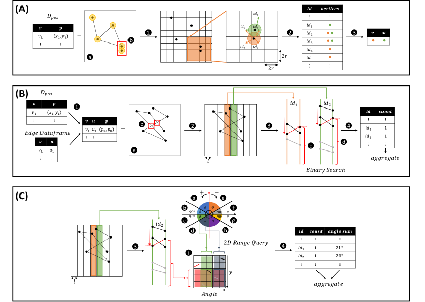
Figure 1: Overview of enhanced readability evaluation algorithms. (A) Node occlusion overview. (B) Edge crossing overview. (C) Edge crossing angle overview. Each number in the circle indicates each step of the algorithm. Note that the first two steps of the edge crossing angle are omitted since they are the same as the first two steps of edge crossing.

The most significant time-consuming task from the previous implementation is the join operation. The join operation with a large number of rows requires an expensive shuffle operation which includes partition transferring with each machine. This is not efficiently computed even with a large number of machines due to network latency. To avoid this, we propose enhanced readability evaluation algorithms using the grid method that divides and conquers multiple independent small problems so that the use of shuffle operations are minimized.

3.2.1 Enhanced Distributed Node Occlusion

Figure 1 (A) shows the overall pipeline of the enhanced node occlusion evaluation algorithm. First, it starts with a given dataframe $D_{pos}$ containing vertices $v_{i}$ and its $xy$-coordinate $p_{i}=(x_{i},y_{i})$. This dataframe can be viewed as vertices placed in a two-dimensional plane with their boundaries (A- ). Each vertex has its boundary which is represented as yellow circles in A- with the same radius. In order to count cases where boundaries are overlapping each other (i.e., A- ) without join operation, grid division (A- ) is conducted. The size of each grid is $2r$ by $2r$ where $r$ denotes the radius of each boundary. By setting grid size to $2r$ square, each vertex’s potential occlusions are all located in adjacent 9 grids including its own grid. To compare each potential occlusion, each vertex is mapped to each grid where its boundary is overlapping. As a result of this process, it now has dataframe containing grid ids and classified vertices for each grid (A- ). Next, it applies group-by operation on the grid id column, and exact $O(n^{2})$ pair-wise comparison is performed for each group with aggregate function for exploding all vertices pairs. This gives us dataframe with vertices pairs overlapping each other including duplicated pairs. Finally, the distinct operation is performed on the dataframe to remove duplicated pairs (A- ). The number of rows in the resulting dataframe is $N_{c}$.

3.2.2 Enhanced Distributed Edge Crossing

Figure 1 (B) shows the overall pipeline of the enhanced edge crossing evaluation algorithm. First of all, it starts with given dataframes $D_{pos}$ and Edge Dataframe which contains vertex id pairs of each edge. And it generates a new dataframe containing each edge’s two vertex ids and their $xy$-coordinates in one row by performing the equal joining $D_{pos}$ with Edge Dataframe on the vertex id column (B- ). The resulting dataframe can be seen as vertices and edges placed in a two-dimensional plane (B- ). In order to count cases where edges are crossing each other (i.e., B- ) without join operation, grid division (B- ) is also conducted with some small width size $l$. But unlike the node occlusion, it divides only vertically to minimize non-comparable pairs. We define two line segments are comparable when both edges have more than one common vertical lines that they’re crossing. If two line segments $s_{1}$ and $s_{2}$ are comparable at vertical lines $l_{1}$ and $l_{2}$, they are considered to be crossed if and only if their relationship between the $y$ coordinates lies on each line is reversed from $l_{1}$ to $l_{2}$. However, if we divide into grids as same as the node occlusion, we can face various situations where two line segments are non-comparable which means they don’t have more than one common vertical grid lines such as a line segment crossing the top of the grid line and right of the grid line, etc. By dividing only vertically, we can minimize such cases and maximize comparable cases at the same time. In order to further minimize non-comparable cases, the grid’s width size $l$ needs to be smaller. Now, edges are divided into smaller line segments for each grid. And it performs group-by operation on each grid, and $O(n\log{n})$ edge crossing counting algorithm is conducted for each group (B- ). The edge counting algorithm uses two data structures to achieve $O(n\log{n})$ edge crossing counting. A sorted array $L$ consisted of the left side’s $y$-coordinates $l_{i}$ and an initially empty balanced binary tree $R$ manages the right side’s $y$-coordinates $r_{i}$ in non-decreasing order. Since we’re only considering cases where every line segment in a group are comparable on the group’s left and right grid lines, it only need to manage $y$-coordinates that each line segment is crossing with the grid lines. It sweeps through the $l_{i}$ of the left grid line in non-decreasing order using $L$ and updates $R$ with the new $r_{i}$ of the currently searching line segment $i$. We can notice that the number of line segments that cross with the currently searching line segment $i$ is the same as the number of the right side’s $y$-coordinates that are greater than $r_{i}$ since they are reversed from the left grid to the right grid with the line segment $i$. For instance, B- and B- indicate line segments that are crossing with the currently searching line segment (red lines). Grey lines indicate not yet searched line segments that are not contained in $R$. Because $R$ is a balanced binary tree, it can binary search to find the number of line segments that are greater than $r_{i}$ and achieve $O(n\log{n})$ time complexity. As a result of this process, it now has a dataframe containing grid ids and the number of crossing lines in each grid (B- ). Finally, the aggregate function for summing up counted values is applied which will return the value of $E_{c}$.

3.2.3 Enhanced Distributed Edge Crossing Angle

Figure 1 (C) shows the overall pipeline of the enhanced edge crossing angle evaluation algorithm. The beginning of this algorithm is the same as the enhanced edge crossing algorithm as shown in Figure 1 B- and B- . After dividing edges into line segments, it uses a sorted array $L$ to sweep the left grid side’s $y$-coordinates $l_{i}$ as same as the enhanced edge crossing algorithm for each group (C- ). But, it uses a 2-dimensional dynamic segment tree as $R$ to manage the right grid side instead of a balanced binary tree. $R$ is updated by two factors that consisting each dimension of the $R$: angle $\theta_{i}$ and $y$-coordinate lies on the right grid side $r_{i}$. $\theta_{i}\in[0,\pi)$ indicates the angle between a line segment $i$ and $x$-axis. For the currently searching line segment $i$, we can group one of the crossing line segments $j$ into one of the 8 angle categories (C- $\sim$ C- ). Each angle category has its angle range relative to the $\theta_{i}$ as follows:

• C- left inner less ($LIL$): $[\theta_{i},\theta_{i}+\vartheta)$

• C- left inner greater ($LIG$): $[\theta_{i}+\vartheta,\theta_{i}+\frac{\pi}{2})$

• C- left outer greater ($LOG$): $[\theta_{i}+\frac{\pi}{2},\theta_{i}+\pi-\vartheta)$

• C- left outer less ($LOL$): $[\theta_{i}+\pi-\vartheta,\theta_{i}+\pi)$

• C- right inner less ($RIL$): $[\theta_{i}-\vartheta,\theta_{i})$

• C- right inner greater ($RIG$): $[\theta_{i}-\frac{\pi}{2},\theta_{i}-\vartheta)$

• C- right outer greater ($ROG$): $[\theta_{i}-\pi+\vartheta,\theta_{i}-\frac{\pi}{2})$

• C- right outer less ($ROL$): $[\theta_{i}-\pi,\theta_{i}-\pi+\vartheta)$

Where $\vartheta$ denotes the ideal angle. And using the sum of each category, we can compute the edge crossing angle for $i$ as Equation 1.

$$\begin{split}\sum_{e_{j}\in c(e_{i})}{\frac{\left|\vartheta-\theta_{e_{i},e_{j}}\right|}{\vartheta}}&=\vartheta|LIL|-(\sum{LIL}-\theta_{i}|LIL|)\\ &+(\sum{LIG}-\theta_{i}|LIG|)-\vartheta|LIG|\\ &+(\theta_{i}|LOG|-(\sum{LOG}-\pi|LOG|))-\vartheta|LOG|\\ &+\vartheta|LOL|-(\theta_{i}|LOL|-(\sum{LOL}-\pi|LOL|))\\ &+\vartheta|RIL|-(\theta_{i}|RIL|-\sum{RIL})\\ &+(\theta_{i}|RIG|-\sum{RIG})-\vartheta|RIG|\\ &+((\sum{ROG}+\pi|ROG|)-\theta_{i}|ROG|)-\vartheta|ROG|\\ &+\vartheta|ROL|-((\sum{ROL}+\pi|ROL|)-\theta_{i}|ROL|)\end{split}$$ (1)

If each angle group contains only angles that all of their corresponding segment $j$ are satisfying $r_{j}$ > $r_{i}$, we can compute the edge crossing angle for currently searching line segment $i$ by using Equation 1. Since $R$ is a 2-dimensional dynamic segment tree with angle and $y$-coordinate dimension, we can get each angle group’s cardinality and summation value with $y$-coordinate condition $r_{j}$ > $r_{i}$ with $O(n\log^{2}{n})$ time complexity. For instance, C- indicates line segments located in each angle group for the currently searching line segment (red line). Grey lines indicate not yet searched line segments. As a result of this step, it has a dataframe containing grid ids and the number of crossing line segments with the sum of crossing angles of the corresponding grid (C- ). Finally, the aggregate function for summing up counted values and crossing angles is applied so that it can directly compute $E_{ca}$.

4 Experiments

Table 1: The number of vertices and edges of each dataset

Dataset	$|V|$	$|E|$	Description
ego-Facebook	4,039	88,234	Facebook social network
musae-facebook	22,470	171,002	Facebook page network
musae-github	37,700	289,003	Github social network
soc-RedditHyperlinks	35,776	286,561	Reddit hyperlinks network
cit-HepTh	27,770	352,807	Arxiv citation network
soc-Epinions1	75,879	508,837	Online social network

Table 2: Computational time in seconds.

		ego-Facebook	musae-facebook	musae-github	soc-RedditHyperlinks	cit-HepTh	soc-Epinions1
Greadability.js	$N_{c}$	0.3	8	24	23	13	103
	$M_{a}$	0.4	0.6	1	0.5	1	1
	$M_{l}$	0.02	0.2	0.07	0.06	0.09	0.9
	$E_{c}$	339	1,828	7,540	6,107	13,771	52,545
	$E_{ca}$	339	1,828	7,540	6,107	13,771	52,545
Spark exact	$N_{c}$	4	14	43	36	22	160
	$M_{a}$	6	4	7	3	4	8
	$M_{l}$	4	3	4	2	3	5
	$E_{c}$	792	2,988	8,641	8,482	12,483	27,115
	$E_{ca}$	882	3,367	9,129	8,813	13,443	30,178
Enhanced algorithm	$N_{c}$	3	2	2	5	2	6
	$E_{c}$	35	64	131	124	129	359
	$E_{ca}$	234	421	1,025	1,047	1,294	1,668

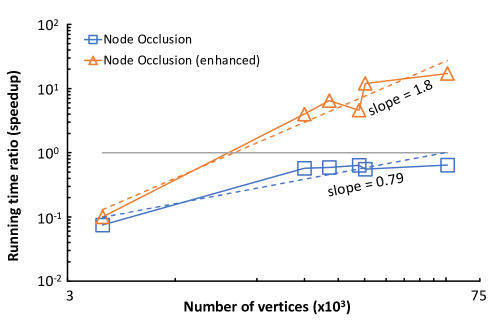
Figure 2: Running time ratio by the number of vertices. Only readability evaluation algorithms whose running time is influenced by the number of vertices are shown. The dotted lines indicate fitted power functions. The grey line indicates $1\times$ improvement where running time becomes the same as $Greadability.js$.

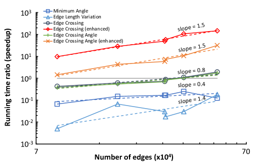
Figure 3: Running time ratio by the number of edges. Only readability evaluation algorithms whose running time is influenced by the number of edges are shown. The dotted lines indicate fitted power functions. The grey line indicates $1\times$ improvement where running time becomes the same as $Greadability.js$.

Table 3: Percentage errors of the enhanced algorithms on random layouts of each dataset. Node occlusion proved its exactness by showing 0% error rates on all datasets. Edge crossing and Edge crossing angle show an average of about 1.5% and 4.5% error rates respectively.

Dataset	ego-Facebook	musae-facebook	musae-github	cit-HepTh	soc-RedditHyperlinks	soc-Epinions1
$N_{c}$	0.0%	0.0%	0.0%	0.0%	0.0%	0.0%
$E_{c}$	1.4%	1.5%	1.5%	1.5%	1.4%	1.4%
$E_{ca}$	4.8%	1.0%	7.9%	5.2%	3.8%	4.4%

Table 4: Mean values and standard deviations of the percentage errors of the edge crossing across 10 different layouts generated by using the Fruchterman-Reingold layout algorithm of the ego-Facebook dataset.

grid size	grid orientation	mean	std
0.10	vertical	4.5%	0.032
	horizontal	6.1%	0.042
	both	4.2%	0.032
0.05	vertical	2.5%	0.019
	horizontal	3.4%	0.024
	both	2.4%	0.018

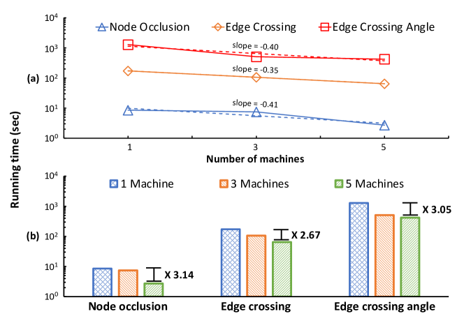
Figure 4: Strong scalability of proposed readability evaluation algorithms on the musae-facebook dataset. The dotted lines on (a) indicate fitted exponential functions.

We conducted quantitative experiments to evaluate the scalability and accuracy of our exact and enhanced algorithms.

Datasets. Six datasets from SNAP Leskovec and Krevl (2014) were used, with vertex counts from 4K to 75K and edge counts from 88K to 508K (Table 1).

Competitors. For Minimum Angle, Edge Crossing, and Edge Crossing Angle, we compared our algorithms against Greadability.js Gove (2018), the only available implementation. For metrics not provided by Greadability.js (Node Occlusion and Edge Length Variation), we implemented single-machine algorithms in JavaScript.

Environments. Our algorithms were tested on Google Cloud Platform Dataproc with six machines (n1-standard-8: 8 vCPUs, 32 GB RAM, 128 GB disk each), while Greadability.js ran on an Intel Core i7-7700 CPU @ 3.60GHz with 64GB RAM.

4.1 Experiment 1: Running Time Comparison

Setup: We measured the running times of Greadability.js, exact algorithms, and enhanced algorithms on random layouts for each dataset, with vertices randomly placed within $x,y\in[0,100]$.

Results: Table 2 shows running times across algorithms. Greadability.js computes $E_{c}$ and $E_{ca}$ together, resulting in identical times for these metrics. Figure 2 and Figure 3 show time ratios relative to Greadability.js by vertex and edge count, respectively. In Figure 2, enhanced Node Occlusion achieves up to $17\times$ speedup, while the exact version remains below $1\times$. In Figure 3, enhanced algorithms achieve up to $146\times$ improvement in Edge Crossing and $31\times$ in Edge Crossing Angle. Exact algorithms require larger graphs for significant speedups, while enhanced algorithms show substantial improvements on smaller graphs.

4.2 Experiment 2: Accuracy Analysis

Setup: To test accuracy, we measured readability metrics using our enhanced algorithms on random layouts and layouts generated with the Fruchterman-Reingold algorithm. Ground-truth values for each metric were computed using straightforward C++ implementations.

Results: Table 3 shows the percentage errors for each dataset. Node Occlusion yielded 0% error as expected. Edge Crossing and Edge Crossing Angle showed averages of 1.5% and 4.5% error, respectively—significantly lower than the deep learning approach Haleem et al. (2019), which reported errors of up to 22.20% and 55%. Accuracy for Edge Crossing and Angle decreases with shorter edge lengths, as these increase non-comparable pairs. We tested Edge Crossing on 10 Fruchterman-Reingold layouts of the ego-Facebook dataset under different grid configurations (see Table 4). Reducing grid size and selecting maximum values across both grid orientations improved accuracy. Despite slight increases in error for layout-generated graphs, accuracy remains much higher than prior methods.

4.3 Experiment 3: Scalability Analysis

Setup: To assess scalability, we measured running times of our enhanced algorithms on the musae-facebook dataset with varying machine counts.

Results: Figure 4 shows strong scalability, with enhanced Node Occlusion and Edge Crossing Angle achieving a slope of about -0.4, meaning doubling machines reduces running time by $2^{0.4}\approx 1.31\times$. All enhanced algorithms showed up to $3.14\times$ speedup as machine counts increased, demonstrating effective scalability for large datasets.

5 Conclusion

The lack of scalable and accurate evaluation algorithms limits our ability to effectively analyze large graph layouts. To address this, we introduced two scalable readability evaluation algorithms—exact and enhanced versions—designed for distributed environments. Our experiments demonstrate that these algorithms offer substantial improvements in running time, accuracy, and scalability for large-scale graphs compared to single-machine approaches. Additionally, we highlighted the practical applicability of our methods through an application in layout optimization, underscoring their value for handling complex graph analysis tasks efficiently.

References

- Henry and Fekete [2007] Nathalie Henry and Jean-Daniel Fekete. Matlink: Enhanced matrix visualization for analyzing social networks. In IFIP Conference on Human-Computer Interaction, pages 288–302. Springer, 2007.
- Li [2015] Wenye Li. Visualizing network communities with a semi-definite programming method. Information Sciences, 321:1–13, 2015.
- Lin et al. [2015] Chun-Cheng Lin, Jia-Rong Kang, and Jyun-Yu Chen. An integer programming approach and visual analysis for detecting hierarchical community structures in social networks. Information Sciences, 299:296–311, 2015.
- Chang et al. [2007] Remco Chang, Mohammad Ghoniem, Robert Kosara, William Ribarsky, Jing Yang, Evan Suma, Caroline Ziemkiewicz, Daniel Kern, and Agus Sudjianto. Wirevis: Visualization of categorical, time-varying data from financial transactions. In 2007 IEEE symposium on visual analytics science and technology, pages 155–162. IEEE, 2007.
- Niu et al. [2018] Zhibin Niu, Dawei Cheng, Liqing Zhang, and Jiawan Zhang. Visual analytics for networked-guarantee loans risk management. In 2018 IEEE Pacific Visualization Symposium (PacificVis), pages 160–169. IEEE, 2018.
- Maçãs et al. [2020] Catarina Maçãs, Evgheni Polisciuc, and Penousal Machado. Vabank: visual analytics for banking transactions. In 2020 24th International Conference Information Visualisation (IV), pages 336–343. IEEE, 2020.
- McGinn et al. [2016] Dan McGinn, David Birch, David Akroyd, Miguel Molina-Solana, Yike Guo, and William J Knottenbelt. Visualizing dynamic bitcoin transaction patterns. Big data, 4(2):109–119, 2016.
- Ke et al. [2004] Weimao Ke, Katy Borner, and Lalitha Viswanath. Major information visualization authors, papers and topics in the acm library. In IEEE symposium on information visualization, pages r1–r1. IEEE, 2004.
- Klammler et al. [2018] Moritz Klammler, Tamara Mchedlidze, and Alexey Pak. Aesthetic discrimination of graph layouts. In International Symposium on Graph Drawing and Network Visualization, pages 169–184. Springer, 2018.
- Gove [2018] Robert Gove. It pays to be lazy: Reusing force approximations to compute better graph layouts faster. 2018.
- Godiyal et al. [2008] Apeksha Godiyal, Jared Hoberock, Michael Garland, and John C Hart. Rapid multipole graph drawing on the gpu. In International Symposium on Graph Drawing, pages 90–101. Springer, 2008.
- Frishman and Tal [2007] Yaniv Frishman and Ayellet Tal. Multi-level graph layout on the gpu. IEEE Transactions on Visualization and Computer Graphics, 13(6):1310–1319, 2007.
- Mi et al. [2016] Peng Mi, Maoyuan Sun, Moeti Masiane, Yong Cao, and Chris North. Interactive graph layout of a million nodes. In Informatics, volume 3, page 23. MDPI, 2016.
- Brinkmann et al. [2017] Govert G Brinkmann, Kristian FD Rietveld, and Frank W Takes. Exploiting gpus for fast force-directed visualization of large-scale networks. In 2017 46th International Conference on Parallel Processing (ICPP), pages 382–391. IEEE, 2017.
- Hinge and Auber [2015] Antoine Hinge and David Auber. Distributed graph layout with spark. In 2015 19th International Conference on Information Visualisation, pages 271–276. IEEE, 2015.
- Arleo et al. [2017] Alessio Arleo, Walter Didimo, Giuseppe Liotta, and Fabrizio Montecchiani. Large graph visualizations using a distributed computing platform. Information Sciences, 381:124–141, 2017.
- Hinge et al. [2017] Antoine Hinge, Gaëlle Richer, and David Auber. Mugdad: Multilevel graph drawing algorithm in a distributed architecture. In Conference on Computer Graphics, Visualization and Computer Vision, page 189, 2017.
- Gómez-Romero et al. [2018] Juan Gómez-Romero, Miguel Molina-Solana, Axel Oehmichen, and Yike Guo. Visualizing large knowledge graphs: A performance analysis. Future Generation Computer Systems, 89:224–238, 2018.
- Haleem et al. [2019] Hammad Haleem, Yong Wang, Abishek Puri, Sahil Wadhwa, and Huamin Qu. Evaluating the readability of force directed graph layouts: A deep learning approach. IEEE computer graphics and applications, 39(4):40–53, 2019.
- Armbrust et al. [2015] Michael Armbrust, Reynold S Xin, Cheng Lian, Yin Huai, Davies Liu, Joseph K Bradley, Xiangrui Meng, Tomer Kaftan, Michael J Franklin, Ali Ghodsi, et al. Spark sql: Relational data processing in spark. In Proceedings of the 2015 ACM SIGMOD international conference on management of data, pages 1383–1394, 2015.
- Dave et al. [2016] Ankur Dave, Alekh Jindal, Li Erran Li, Reynold Xin, Joseph Gonzalez, and Matei Zaharia. Graphframes: an integrated api for mixing graph and relational queries. In Proceedings of the fourth international workshop on graph data management experiences and systems, pages 1–8, 2016.
- Purchase [2002] Helen C Purchase. Metrics for graph drawing aesthetics. Journal of Visual Languages & Computing, 13(5):501–516, 2002.
- Dunne et al. [2015] Cody Dunne, Steven I Ross, Ben Shneiderman, and Mauro Martino. Readability metric feedback for aiding node-link visualization designers. IBM Journal of Research and Development, 59(2/3):14–1, 2015.
- Huang et al. [2008] Weidong Huang, Seok-Hee Hong, and Peter Eades. Effects of crossing angles. In 2008 IEEE Pacific Visualization Symposium, pages 41–46. IEEE, 2008.
- Zaharia et al. [2016] Matei Zaharia, Reynold S Xin, Patrick Wendell, Tathagata Das, Michael Armbrust, Ankur Dave, Xiangrui Meng, Josh Rosen, Shivaram Venkataraman, Michael J Franklin, et al. Apache spark: a unified engine for big data processing. Communications of the ACM, 59(11):56–65, 2016.
- Dean and Ghemawat [2008] Jeffrey Dean and Sanjay Ghemawat. Mapreduce: simplified data processing on large clusters. Communications of the ACM, 51(1):107–113, 2008.
- Fruchterman and Reingold [1991] Thomas MJ Fruchterman and Edward M Reingold. Graph drawing by force-directed placement. Software: Practice and experience, 21(11):1129–1164, 1991.
- Arleo et al. [2018] Alessio Arleo, Walter Didimo, Giuseppe Liotta, and Fabrizio Montecchiani. A distributed multilevel force-directed algorithm. IEEE Transactions on Parallel and Distributed Systems, 30(4):754–765, 2018.
- Leskovec and Krevl [2014] Jure Leskovec and Andrej Krevl. SNAP Datasets: Stanford large network dataset collection. http://snap.stanford.edu/data, June 2014.