A Probabilistic Framework for Estimating the Modal Age at Death

Abstract

The modal age at death is a critical measure for understanding longevity and mortality patterns. However, existing methods primarily focus on point estimates, overlooking the inherent variability and uncertainty in mortality data. This study addresses this gap by introducing a probabilistic framework for estimating the probability distribution of the modal age at death. Using a multinomial model for age-specific death counts and leveraging a Gaussian approximation, our methodology captures variability while aligning with the categorical nature of mortality data. Application to mortality data from six countries (1960–2020) reinforces the framework’s effectiveness in revealing gender differences, temporal trends, and variability across populations. By quantifying uncertainty and improving robustness to data fluctuations, this approach offers valuable insights for demographic research and policy planning.
Keywords: Modal age at death, probabilistic framework, multinomial distribution, demographic analysis, mortality patterns

1 Context and Motivation

In recent decades, survival at older ages has improved dramatically, pushing human longevity further than ever before. While life expectancy often takes center stage, shifts in longevity are more precisely captured by the modal age at death—the age where the highest number of deaths occur in a population. As highlighted by Canudas-Romo, (2008), the modal age at death is a key indicator of population aging and a critical measure of longevity, reflecting the postponement of deaths to older ages under the shifting mortality hypothesis, and providing insights into aging patterns, and lifespan trends, which are essential for accurate demographic forecasting and policy planning. However, estimating the modal age at death is challenging due to the discrete nature of mortality data and the inherent variability in mortality patterns (Kannisto,, 2001; Horiuchi et al.,, 2013).

Several methods have been proposed to estimate the modal age at death. Parametric models, such as the Gompertz, Weibull, and logistic models, have traditionally been used to estimate mortality patterns, with the mode derived analytically from these models. These approaches often emphasize adult mortality patterns and provide insights into aging dynamics (Kannisto,, 2001; Canudas-Romo,, 2008; Missov et al.,, 2015). However, they assume specific functional forms, which may not adequately capture all features of the data.

Non-parametric approaches have emerged as flexible alternatives, relying on smoothing techniques such as kernel smoothing and splines to estimate mortality rates and the modal age without assuming a specific distributional shape (Delwarde et al.,, 2007; Ouellette and Bourbeau,, 2011; Horiuchi et al.,, 2013). These methods have been particularly effective in identifying trends in mortality compression and shifting mortality patterns across different populations.

Canudas-Romo, (2008) introduced an analytical framework for studying the modal age at death, focusing on its relationship with life table functions such as $l(x)$ (survivors) and $d(x)$ (deaths). He derived mathematical expressions to estimate the mode and explored its role in capturing mortality patterns, particularly in the context of the shifting mortality hypothesis.

More recently, Vazquez-Castillo et al., (2024) proposed a novel method based on the mathematical properties of the mode, the discretized derivative test (DDT) method, which offers a computationally efficient way to estimate the modal age in discrete mortality data while avoiding the complexities of smoothing techniques. This method complements the work of Canudas-Romo, (2008) by building on his emphasis on the modal age’s importance within the shifting mortality hypothesis and extending its application as a longevity indicator through a refined, practical estimation approach.

Despite these advances, existing methods primarily focus on point estimates of the mode, often overlooking its variability and uncertainty. A probabilistic framework is needed to capture these aspects, particularly within a discrete mortality context. Brillinger, (1986) introduced a Poisson-based approach for analyzing mortality rates, aligning with the discrete nature of death counts across age intervals. Building on this foundation, we extend the analysis to model age-specific death counts as a multinomial experiment under the assumption of a fixed total number of deaths. This assumption bridges the Poisson framework with multinomial modeling, providing a natural fit for categorical mortality data.

In this paper we propose a simple yet efficient method to estimate the empirical probability distribution of the modal age at death within a discrete framework. Age-specific death counts are framed as outcomes of a multinomial distribution, reflecting their dependence on the total number of deaths. The Lexis diagram offers a conceptual foundation, justifying this multinomial approach by illustrating how deaths are distributed across age intervals in a discrete age-time structure (e.g., Preston et al.,, 2001). Additionally, we discuss the Gaussian approximation of the multinomial distribution for large sample sizes, allowing computationally feasible estimation of the modal age distribution.

Unlike traditional methods, our approach explicitly accounts for the variability in death counts, and provides a probabilistic perspective on the uncertainty surrounding the modal age at death. This probabilistic assessment enhances our understanding of mortality dynamics and offers a robust tool for demographic analysis.

2 Probabilistic Approach for Modal Age Estimation

Existing methodologies often model death counts across age intervals as independent Poisson random variables, an approach supported by Brillinger, (1986). This assumption captures the stochastic variability in mortality data by treating the number of deaths within each age category as outcomes of independent Poisson processes. However, when the total number of deaths $n$ is fixed—for instance, as observed in population—this framework transitions naturally into a multinomial distribution.

The connection between the Poisson and multinomial frameworks arises from the properties of the Poisson distribution. If death counts in each age interval are modeled as independent Poisson random variables, their sum also follows a Poisson distribution. When this total is fixed, the distribution of deaths across age intervals can be understood as a multinomial allocation, where the fixed total $n$ is distributed across age categories based on probabilities that correspond to the expected proportions of deaths in each category (e.g., Bishop et al.,, 2007). This multinomial framework aligns well with the categorical nature of age-specific mortality data.

The Lexis triangle offers a conceptual foundation for this approach. By representing mortality data in a two-dimensional age-time plane, the Lexis diagram naturally illustrates how deaths can be categorized into discrete age intervals, allowing a probabilistic interpretation of their distribution under a fixed total (e.g., Preston et al.,, 2001). Grounded in this concept, we extend the Poisson-based framework by adopting the multinomial model for age-specific death counts. This probabilistic perspective allows us to capture the dependencies among age-specific death counts due to the fixed total, while also accounting for the variability in the data.

2.1 Multinomial Model for Mortality Data

Let $K$ denote the total number of distinct age intervals (or age categories) under consideration. For each age interval $x=1,2,\dots,K$, let $D_{x}$ represent the count of deaths occurring in the age interval $[x,x+1)$. We define the vector of death counts as $\bm{D}=(D_{1},D_{2},\dots,D_{K})^{\top}$. The total number of deaths across all age intervals is $n=D_{1}+D_{2}+\cdots+D_{K}$.

Assuming that each death is an independent trial resulting in one of the $K$ age categories with probabilities $\bm{p}=(p_{1},p_{2},\dots,p_{K})^{\top}$, the vector $\bm{D}$ follows a multinomial distribution:

$$\bm{D}\sim\text{Multinomial}(n,\bm{p}),$$

where $p_{x}$ is the probability that a death occurs in age interval $x$ and these probabilities satisfy $p_{1}+p_{2}+\cdots+p_{K}=1$. These probabilities are typically estimated using life table methods, which adjust for age-specific exposures and mortality rates.

The multinomial distribution is appropriate for modeling scenarios where there are a fixed number of independent trials, each resulting in exactly one of several possible outcomes, with constant probabilities for each outcome (e.g., Bishop et al.,, 2007). In the context of mortality data:

First, each death is treated as an independent trial that results in one of $K$ age categories. The assumption of independence implies that the occurrence of one death does not influence the occurrence of another. While in reality, deaths may not be entirely independent due to factors such as epidemics or social interactions, for large populations and over short time intervals, this assumption can be a reasonable approximation.

Second, the age categories are mutually exclusive and collectively exhaustive. Each death is assigned to exactly one age interval, and all possible age intervals are included, ensuring that every death is accounted for in the analysis.

Third, the probabilities $\bm{p}=(p_{1},p_{2},\dots,p_{K})^{\top}$ are derived using a life table approach. Specifically, $p_{x}$ represents the proportion of individuals who die during the age interval $x$, calculated based on exposure and mortality rates. In life tables, $p_{x}$ is directly proportional to $d_{x}$, the number of deaths during age $x$, as both describe the distribution of deaths but in different forms. To avoid confusion, it is important to note that while $p_{x}$ is scaled to ensure the probabilities sum to 1 ($\sum_{x}p_{x}=1$), $d_{x}$ represents absolute death counts. This scaling reflects the multinomial nature of $p_{x}$, which assigns probabilities over the age intervals. These probabilities are assumed to remain constant throughout the observed period, implying that age-specific mortality rates do not change within each age interval.

It’s important to note that while the individual lifetimes (trials) are assumed to be independent, the counts across age categories $D_{x}$ are dependent because they sum to the fixed total $n$. An increase in deaths in one age category must be offset by decreases in others to maintain the total number of deaths. This dependency is inherent in the multinomial distribution and is reflected in the covariance structure of the counts (e.g., Feller,, 1991).

By modeling the death counts using the multinomial distribution, we capture the discrete and categorical nature of age-specific mortality data. The model accounts for the fixed total number of deaths $n$ and incorporates the dependency of death counts across age categories due to the constraint $D_{1}+D_{2}+\cdots+D_{K}=n$. Moreover, the multinomial model naturally reflects the variability in death counts arising from random fluctuations in mortality, providing a probabilistic framework for analyzing age-specific death distribution.

2.2 Gaussian Approximation for Large Populations

For large values of $n$, the multinomial distribution can be approximated by a multivariate normal distribution due to the multivariate central limit theorem (e.g., Muirhead,, 2009). This Gaussian approximation simplifies computations and enables analytical methods for estimating probabilities that might be complex to calculate exactly, especially when the number of age categories $K$ is large.

The central limit theorem states that as $n$ approaches infinity, the distribution of properly normalized sums of independent random variables converges to a normal distribution. In the case of the multinomial distribution, if $n$ is large and each expected count $np_{x}$ is sufficiently large, the distribution of the death counts $\bm{D}$ can be approximated by a multivariate normal distribution.

Under these conditions, $\bm{D}$ is approximated as:

$$\bm{D}\approx\mathcal{N}(\bm{\mu},\bm{\Sigma}),$$

where $\bm{\mu}=n\bm{p}$ is the mean vector, representing the expected number of deaths at each age interval, and $\bm{\Sigma}=n\left(\text{Diag}(\bm{p})-\bm{p}\bm{p}^{\top}\right)$ is the covariance matrix, capturing the variances and covariances between age categories.

The requirement for large $n$ ensures that the normal approximation is accurate. Additionally, it is important that each expected count, which avoids issues with skewness or discreteness that can affect the approximation. If any $p_{x}$ is very small, the corresponding component of $\bm{D}$ may not be well-approximated by a normal distribution.

The covariance matrix $\bm{\Sigma}$ reflects the negative correlations between counts in different age categories, arising because the total number of deaths $n$ is fixed; an increase in deaths in one age category must be followed by a decrease in another to maintain the total. By using the Gaussian approximation, we can perform computations and estimations that are otherwise difficult with the exact multinomial distribution, facilitating the estimation of the probability distribution of the modal age at death.

2.3 Probabilistic Estimation of the Modal Age

Our goal is to estimate the probability that age $x$ is the modal age—the age with the highest death count. Using the Gaussian approximation, we can approach this problem analytically or through computational methods.

Let us define $M$ as the modal age at death. By definition, the death count at age $M$ is the maximum among all age categories, which means that $\mathbb{P}(D_{M}\geq D_{x})=1$ for all $x=1,\dots,K$. In the discrete setting of age intervals, calculating this probability can be more manageable than in a continuous framework.

We aim to find $\mathbb{P}(M=x)=\mathbb{P}\left(D_{x}=\max(D_{1},D_{2},\dots,D_{K})\right)$, which is the probability that $D_{x}$ is the largest among all components of the death count vector $\bm{D}$. This probability can be expressed as:

$$\mathbb{P}(M=x)=\mathbb{P}(D_{x}-D_{j}\geq 0\text{ for all }j\neq x).$$

Since $\bm{D}$ follows a multivariate Gaussian distribution with mean vector $\bm{\mu}$ and covariance matrix $\bm{\Sigma}$, any linear combination of its components will also be normally distributed. Specifically, if we define the differences $Y_{x,j}=D_{x}-D_{j}$ for each $j\neq x$, each $Y_{x,j}$ is a normally distributed random variable with mean and variance given by:

$$\mu_{x,j}=\mu_{x}-\mu_{j},\quad\sigma_{x,j}^{2}=\sigma_{xx}+\sigma_{jj}-2\sigma_{xj},$$

where $\sigma_{ij}$ represents the covariance between $D_{i}$ and $D_{j}$.

The set of differences $\bm{Y}_{x}=\{Y_{x,j}:j\neq x\}$ are jointly normally distributed random variables. We are interested in the probability that all these differences are non-negative, meaning that $D_{x}$ is greater than or equal to each $D_{j}$ for $j\neq x$.

These differences can be represented collectively as:

$$\bm{Y}_{x}\sim\mathcal{N}(\bm{\Lambda}_{x}\bm{\mu},\bm{\Lambda}_{x}\bm{\Sigma}\bm{\Lambda}_{x}^{\top}),$$

where $\bm{\Lambda}_{x}$ is a transformation matrix that maps the mean vector $\bm{\mu}$ of $\bm{D}$ to the mean of $\bm{Y}_{x}$ by capturing the difference structure. Specifically, $\bm{\Lambda}_{x}$ has dimensions $(K-1)\times K$, with each row corresponding to the difference $D_{x}-D_{j}$. The entries of $\bm{\Lambda}_{x}$ are defined as:

$$\lambda_{x,i,k}=\mathbb{I}(k=x)-\mathbb{I}(k=j_{i}),$$

where $j_{i}$ denotes the $i$-th index not equal to $x$, and $\mathbb{I}(\cdot)$ is the indicator function.

Therefore, for each age $x$, the probability that $x$ is the modal age is given by:

$$\mathbb{P}(M=x)=\int_{R_{x}}f_{\bm{Y}_{x}}(\bm{y}_{x})\,d\bm{y}_{x},$$ (1)

where $f_{\bm{Y}_{x}}(\bm{y}_{x})$ is the joint multivariate normal density function of $\bm{Y}_{x}$, and the integration region $R_{x}$ is defined as:

$$R_{x}=\{\bm{y}_{x}\in\mathbb{R}^{K-1}\mid Y_{x,j}\geq 0\text{ for all }j\neq x\}.$$

Evaluating this integral involves integrating over a $(K-1)$-dimensional space with boundaries defined by the inequalities $Y_{x,j}\geq 0$. As $K$ increases, the dimensionality of the integration space grows, making exact computation increasingly challenging.

Several methods exist for calculating multivariate normal probabilities over such regions, including numerical integration, orthant probabilities, and approximation techniques (Genz and Bretz,, 2009). However, these methods become computationally intensive as the number of dimensions increases. In our context, where $K$ can be large (e.g., the number of age intervals in mortality data), these methods may not be practical.

An alternative is to use computational methods to approximate these probabilities. Software packages like mvtnorm in R provide functions to numerically compute multivariate normal probabilities (Mi et al.,, 2009). By leveraging these tools, we can estimate $\mathbb{P}(M=x)$ without performing the high-dimensional integral analytically. This computational approach allows us to handle larger values of $K$ and obtain accurate estimates of the probability distribution of the modal age at death.

Algorithm 1 summarizes the estimation procedure, outlining the steps for estimating the probability distribution of the modal age at death. By calculating age-specific probabilities, and identifying the modal age across the death distribution, this approach provides an empirical estimate of the modal probabilities. The algorithm is structured to ensure convergence of the estimated probabilities as the total number of deaths $n$ increases.

Input: $\bm{D_{x}}$: Vector of death counts for each age interval, $\bm{E_{x}}$: Vector of exposures for each age interval, $\bm{x}$: Vector of age intervals

Output: Data frame with mode, probability for each mode, and cumulative probability

1

2Compute total deaths $n\leftarrow\text{sum}(\bm{D_{x}})$ ;

3 Calculate $\bm{d_{x}}$ using life table methods for a cohort of size 1 ;

4 Set $\bm{p}\leftarrow\bm{d_{x}}$ ;

5

6Define mean vector $\bm{\mu}\leftarrow n\cdot\bm{p}$ and covariance matrix $\bm{\Sigma}\leftarrow n\cdot(\text{diag}(\bm{p})-\bm{p}\cdot\bm{p}^{\top})$ ;

7 for each $k$ in $\bm{x}$ do

8       Construct difference matrix $\bm{\Lambda}_{k}$ for comparisons between $X_{k}$ and $X_{j}$, $j\neq k$ ;

9       Compute covariance matrix of differences $\bm{\Sigma}_{k}\leftarrow\bm{\Lambda}_{k}\cdot\bm{\Sigma}\cdot\bm{\Lambda}_{k}^{\top}$ ;

10       Compute mean vector $\bm{\mu}_{k}\leftarrow\bm{\Lambda}_{k}\cdot\bm{\mu}$ ;

11       Calculate $\mathbb{P}(M=k)$ by solving the integral in Equation 1 and store it;

12      

13 end for

14

15If using numerical methods, normalize the estimated discrete probability density to ensure that $\sum_{k}\mathbb{P}(M=k)=1$ ;

return The estimated discrete probability density $\mathbb{P}(M=k)$

Algorithm 1 Mode Distribution Estimation Algorithm

In the Algorithm 1, the vector $\bm{d_{x}}$ is computed using life table methods for a normalized cohort of size 1. In this context, $\bm{d_{x}}$ represents the proportions of individuals who die during the age intervals. This normalization process ensures that all probabilities and rates are expressed as fractions of the initial cohort size, providing a standardized perspective for the analysis (e.g., Preston et al.,, 2001).

To ensure the probabilities form a valid distribution, we normalize them so their total sums to 1. This step corrects potential inaccuracies from numerical methods, such as pmvnorm from the package mvtnorm in R, where approximation errors may cause deviations. Normalization preserves relative proportions while ensuring consistency and interpretability as a valid probability distribution.

2.4 Convergence of the Modal Distribution as $n$ Increases

An important property of our probabilistic framework is that as the total number of deaths $n$ increases, the probability distribution of the modal age at death converges to a point mass at the age interval with the highest underlying death probability. This follows from the fact that the modal age at death, by definition, is the age where the number of deaths is the highest. Since the age-specific death probabilities represent the expected proportion of deaths at each age interval, we naturally expect the age interval containing the real modal age to also have the maximum value of $p_{x}$.

However, it is important to distinguish between the real modal age (a precise value) and the interval containing it. While the real modal age may not align perfectly with the midpoint of the interval, in practical applications, the discrete framework requires us to assign it to an interval. Thus, the age interval with the highest $p_{x}$ serves as a probabilistic approximation, as $p_{x}$ reflects the expected relative frequency of deaths within each interval. As $n$ increases, this approximation improves, and the interval with the highest $p_{x}$ converges to the true modal interval, making $p_{x}$ a robust proxy for identifying the modal age.

We formalize this result in the following proposition.

Proposition 1.

Let $x^{\star}$ denote the age interval with the highest probability $p_{x^{\star}}$, and suppose that $p_{x^{\star}}>p_{j}$ for all $j\neq x^{\star}$. As the total number of deaths $n$ increases, the probability distribution of the modal age at death converges to a point mass at the age interval $x^{\star}$ with the highest underlying death probability $p_{x^{\star}}$, i.e.,

$$\lim_{n\to\infty}\mathbb{P}(M=x^{\star})=1,$$

where $M$ is the modal age at death. This result implies that the real modal age falls within the interval $x^{\star}$ as $n$ becomes large.

Proof.

Consider the random variables $D_{x}$ representing the number of deaths in age interval $x$. Under the multinomial distribution, the counts $D_{x}$ satisfy:

$$\mathbb{E}\left[\frac{D_{x}}{n}\right]=p_{x},\quad\text{Var}\left(\frac{D_{x}}{n}\right)=\frac{p_{x}(1-p_{x})}{n}.$$

By the Weak Law of Large Numbers, the sample proportions $\frac{D_{x}}{n}$ converge in probability to the true probabilities $p_{x}$ as $n\to\infty$:

$$\frac{D_{x}}{n}\xrightarrow{\mathbb{P}}p_{x}.$$

At $x^{\star}$ we have that $p_{x^{\star}}=\max\{p_{1},p_{2},\dots,p_{K}\}$. Since $p_{x^{\star}}>p_{j}$ for all $j\neq x^{\star}$, there exists a positive constant $\delta$ such that:

$$p_{x^{\star}}-p_{j}\geq\delta>0,\quad\forall j\neq x^{\star}.$$

By the convergence in probability, for any $\epsilon>0$ and sufficiently large $n$, there exists $N$ such that for all $n>N$:

$$\mathbb{P}\left(\left|\frac{D_{x^{\star}}}{n}-p_{x^{\star}}\right|<\frac{\delta}{3}\right)>1-\frac{\epsilon}{2},$$

and for each $j\neq x^{\star}$:

$$\mathbb{P}\left(\left|\frac{D_{j}}{n}-p_{j}\right|<\frac{\delta}{3}\right)>1-\frac{\epsilon}{2K}.$$

By the union bound, the probability that all these events occur simultaneously is greater than $1-\epsilon$:

$$\mathbb{P}\left(\left|\frac{D_{x^{\star}}}{n}-p_{x^{\star}}\right|<\frac{\delta}{3},\,\bigcap_{j\neq x^{\star}}\left|\frac{D_{j}}{n}-p_{j}\right|<\frac{\delta}{3}\right)>1-\epsilon.$$

When these events occur, we have:

$$\frac{D_{x^{\star}}}{n}>p_{x^{\star}}-\frac{\delta}{3},$$

and for each $j\neq x^{\star}$:

$$\frac{D_{j}}{n}<p_{j}+\frac{\delta}{3}\leq p_{x^{\star}}-\delta+\frac{\delta}{3}=p_{x^{\star}}-\frac{2}{3}\delta.$$

Therefore, for all $j\neq x^{\star}$:

$$\frac{D_{x^{\star}}}{n}-\frac{D_{j}}{n}>\left(p_{x^{\star}}-\frac{\delta}{3}\right)-\left(p_{x^{\star}}-\frac{2}{3}\delta\right)=\frac{\delta}{3}>0.$$

This implies that $D_{x^{\star}}>D_{j}$ for all $j\neq x^{\star}$. Thus,

$$\mathbb{P}\left(D_{x^{\star}}>D_{j}\text{ for all }j\neq x^{\star}\right)>1-\epsilon.$$

Since $\epsilon$ is arbitrary, we take $\epsilon\downarrow 0$ and conclude that:

$$\lim_{n\to\infty}\mathbb{P}\left(D_{x^{\star}}>D_{j}\text{ for all }j\neq x^{\star}\right)=1.$$

Therefore,

$$\lim_{n\to\infty}\mathbb{P}(M=x^{\star})=1.$$

∎

This result shows that, as the total number of deaths $n$ becomes large, the modal age at death converges in probability to the age interval $x^{\star}$ with the highest death probability $p_{x^{\star}}$. Consequently, the distribution of the mode becomes increasingly concentrated in the age interval that contains the true modal age, ensuring the consistency of our method within the multinomial framework. Unlike methods that rely on the derivative of an estimated density function, our approach avoids challenges associated with identifying local maxima or handling saddle points.

For finite $n$, however, variability in the data due to random fluctuations can result in uncertainty about the modal age. Estimating the probability distribution of the mode allows us to capture this uncertainty, providing clearer picture of the likelihood that each age interval contains the mode. This is particularly useful in practical settings, such as when the differences between $p_{x^{\star}}$ and $p_{j}$ for $j\neq x^{\star}$ are not large.

2.5 Extension to a Continuous Framework

It is worth noting that while our approach is formulated within a discrete framework of age intervals, a similar methodology can be considered in a continuous setting. As the number of age intervals $K$ increases and the width of each interval decreases, the discrete age categories approach a continuous age variable. In the limit as $K\to\infty$, the multinomial distribution over discrete categories transitions to a continuous distribution over age (Seeger,, 2004).

In this continuous framework, the death counts can be modeled using a Poisson point process or, under certain conditions, approximated by a Gaussian process due to the central limit theorem (e.g., Daley et al.,, 2003). Specifically, the cumulative death counts over age can be considered as a realization of a stochastic process with a continuous index set. The differences $Y_{x,j}=D_{x}-D_{j}$ between age-specific death counts would then correspond to increments of this process.

The challenge in the continuous case lies in defining the probability that a particular age $x$ is the mode since, in a continuous distribution, the probability of observing any exact value is zero. However, we can consider the probability density function of the age at death and analyze the behavior of the process around its maximum (e.g., Adler and Taylor,, 2009). Techniques from stochastic process theory, such as studying the maxima of Gaussian processes, can be employed.

Extending our method to the continuous framework would involve modeling the death counts as a Gaussian process over age and calculating the distribution of the age at which the process attains its maximum. While this introduces additional mathematical complexity, it offers a more precise representation of mortality patterns when age is treated as a continuous variable.

However, practical implementation of such an approach requires careful consideration of the covariance structure of the process and computational methods for handling continuous Gaussian processes (e.g., Seeger,, 2004). In many applications, the discrete framework provides a sufficiently accurate approximation, especially when age intervals are small. Nonetheless, exploring the continuous analog of our method could be a valuable direction for future research, potentially leveraging advancements in the analysis of Gaussian processes and extreme value theory.

3 Empirical Application

To validate our methodology, we applied it to actual mortality data from six countries: Denmark, France, Italy, Japan, Netherlands, and United States (US), covering the period from 1960 to 2020, obtained from the Human Mortality Database, (2024). We analyzed female and male populations separately to investigate gender differences in the modal age at death. This dataset provides a robust basis for evaluating the applicability of our method to real-world scenarios, given the varying population sizes, cultural contexts, and mortality patterns across these nations.

The results, presented in Figure 1, show an overall upward trend in the modal age at death from 1960 to 2020 across the six analyzed countries. This trend reflects consistent improvements in longevity over time. Notably, we observe gender-specific differences, with females consistently presenting a higher modal age at death than males, underscoring the persistent gender gap in longevity.

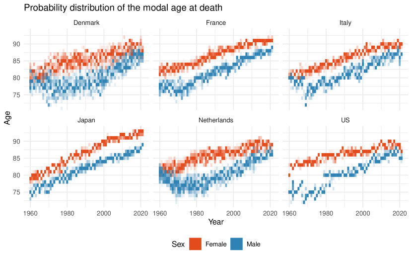
Figure 1: Modal age at death from 1960 to 2020 across six countries (Denmark, France, Italy, Japan, Netherlands, and the United States) by gender (female and male). The heatmap represents the probability distribution of the modal age at death for each year, with higher color intensities indicating greater probabilities of a specific age being the modal value. The upward trend reflects improvements in longevity, while broader distributions in Denmark and the Netherlands suggest greater variability, likely due to smaller populations. In contrast, Japan and Italy show narrower, more consistent distributions.

Some fluctuations are visible in the distribution, with temporary plateaus or slight declines in the mode occurring during specific periods. For example, certain countries show slower progress or even minor declines in modal age at death during the late 1990s and early 2000s, possibly linked to region-specific socio-economic or health crises.

Among the countries analyzed, Japan stands out with a particularly high and steadily increasing modal age at death, reflecting the nation’s advanced healthcare system and lifestyle factors. In contrast, the United States exhibits more variability, particularly in recent decades, which could be attributed to healthcare inequalities and the broader impact of external factors, such as the opioid crisis and the COVID-19 pandemic.

The figure also highlights variability in the distribution shapes. Broader distributions, particularly in Denmark and the Netherlands, point to greater statistical uncertainty, potentially tied to smaller population sizes. Meanwhile, narrower distributions in countries like Japan suggest more stable and consistent modal age estimates, highlighting the importance of considering variability when interpreting the distribution of the mode.

Overall, the application of this methodology to mortality data across diverse national contexts highlights its utility in capturing trends and disparities in the modal age at death. By showcasing the full probability distribution of the modal age at death, it provides better picture of the dynamics of longevity and its improvements across populations.

4 Concluding Remarks and Future Directions

We introduced a probabilistic framework for estimating the distribution of modal age at death, using the multinomial distribution and its Gaussian approximation. By modeling age-specific death counts as outcomes of a multinomial experiment and incorporating the dependency among counts due to the fixed total number of deaths, our method provides an empirical estimate of the probability distribution of the modal age. This approach aligns with the discrete nature of mortality data and addresses the variability often overlooked by traditional point-estimation methods.

The application of our methodology to real-world mortality data from six countries highlighted its ability to capture longevity patterns, including temporal trends and gender differences in modal age. Additionally, the framework’s robustness in reflecting the uncertainty surrounding the modal age offers a valuable tool for demographic analysis, especially in contexts with smaller populations or fluctuating mortality patterns.

Nevertheless, our method is not without limitations. It is sensitive to population shocks, such as pandemics or sudden socio-economic disruptions, which can affect the estimation of age-specific probabilities $\bm{p}$. While these limitations do not undermine the utility of the method, they highlight areas for future improvement. Specifically, integrating Monte Carlo methods or Bayesian frameworks to account for variability in the mortality rates could enhance the model’s robustness to mortality shocks. For smaller populations, hierarchical models or methods that address overdispersion, such as the negative binomial or Bell distribution, may provide more reliable estimates.

Another avenue for future research is extending the framework to a continuous setting. While the discrete framework used here is practical and closely mirrors real-world mortality data, continuous models could provide a more nuanced understanding of mortality dynamics. Gaussian processes and methods from extreme value theory may offer promising directions for analyzing the distribution of the mode in continuous age contexts.

In conclusion, our method introduces a significant innovation by providing the first empirical framework for estimating the probability distribution of the modal age at death within a discrete context. By moving beyond traditional point estimates, this approach offers a probabilistic perspective that explicitly quantifies variability, reveals competing age intervals, and improves robustness to data fluctuations. By aligning with the categorical nature of mortality data, it enhances our ability to analyze and interpret mortality patterns across diverse contexts, offering valuable insights for a better understanding of population dynamics.

References

- Adler and Taylor, (2009) Adler, R. J. and Taylor, J. E. (2009). Random fields and geometry. Springer Science & Business Media.
- Bishop et al., (2007) Bishop, Y. M., Fienberg, S. E., and Holland, P. W. (2007). Discrete multivariate analysis: Theory and practice. Springer Science & Business Media.
- Brillinger, (1986) Brillinger, D. R. (1986). A biometrics invited paper with discussion: the natural variability of vital rates and associated statistics. Biometrics, pages 693–734.
- Canudas-Romo, (2008) Canudas-Romo, V. (2008). The modal age at death and the shifting mortality hypothesis. Demographic Research, 19:1179–1204.
- Daley et al., (2003) Daley, D. J., Vere-Jones, D., et al. (2003). An introduction to the theory of point processes: volume I: elementary theory and methods. Springer.
- Delwarde et al., (2007) Delwarde, A., Denuit, M., and Eilers, P. (2007). Smoothing the lee–carter and poisson log-bilinear models for mortality forecasting: a penalized log-likelihood approach. Statistical modelling, 7(1):29–48.
- Feller, (1991) Feller, W. (1991). An introduction to probability theory and its applications, Volume 2, volume 81. John Wiley & Sons.
- Genz and Bretz, (2009) Genz, A. and Bretz, F. (2009). Computation of multivariate normal and t probabilities, volume 195. Springer Science & Business Media.
- Horiuchi et al., (2013) Horiuchi, S., Ouellette, N., Cheung, S. L. K., and Robine, J.-M. (2013). Modal age at death: lifespan indicator in the era of longevity extension. Vienna Yearbook of Population Research, pages 37–69.
- Human Mortality Database, (2024) Human Mortality Database (2024). Human mortality database, hmd. Max Planck Institute for Demographic Research (Germany), University of California, Berkeley (USA), and French Institute for Demographic Studies (France). Available at: http://www.mortality.org/. Extract on: November 11, 2024.
- Kannisto, (2001) Kannisto, V. (2001). Mode and dispersion of the length of life. Population: An English Selection, pages 159–171.
- Mi et al., (2009) Mi, X., Miwa, T., and Hothorn, T. (2009). mvtnorm: New numerical algorithm for multivariate normal probabilities. R Journal 1 (2009), Nr. 1, 1(1):37–39.
- Missov et al., (2015) Missov, T. I., Lenart, A., Nemeth, L., Canudas-Romo, V., and Vaupel, J. W. (2015). The gompertz force of mortality in terms of the modal age at death. Demographic Research, 32:1031–1048.
- Muirhead, (2009) Muirhead, R. J. (2009). Aspects of multivariate statistical theory. John Wiley & Sons.
- Ouellette and Bourbeau, (2011) Ouellette, N. and Bourbeau, R. (2011). Changes in the age-at-death distribution in four low mortality countries: A nonparametric approach. Demographic Research, 25:595–628.
- Preston et al., (2001) Preston, S., Heuveline, P., and Guillot, M. (2001). Demography: Measuring and modeling population processes. Blackwell, Malden.
- Seeger, (2004) Seeger, M. (2004). Gaussian processes for machine learning. International journal of neural systems, 14(02):69–106.
- Vazquez-Castillo et al., (2024) Vazquez-Castillo, P., Bergeron-Boucher, M.-P., and Missov, T. I. (2024). Longevity à la mode: A discretized derivative tests method for accurate estimation of the adult modal age at death. Demographic Research, 50:325–346.