Modelling Population-Level Hes1 Dynamics: Insights from a Multi-Framework Approach

Abstract

Mathematical models of living cells have been successively refined with advancements in experimental techniques. A main concern is striking a balance between modelling power and the tractability of the associated mathematical analysis.

In this work we model the dynamics for the transcription factor Hairy and enhancer of split-1 (Hes1), whose expression oscillates during neural development, and which critically enables stable fate decision in the embryonic brain. We design, parametrise, and analyse a detailed spatial model using ordinary differential equations (ODEs) over a grid capturing both transient oscillatory behaviour and fate decision on a population-level. We also investigate the relationship between this ODE model and a more realistic grid-based model involving intrinsic noise using mostly directly biologically motivated parameters.

While we focus specifically on Hes1 in neural development, the approach of linking deterministic and stochastic grid-based models shows promise in modelling various biological processes taking place in a cell population. In this context, our work stresses the importance of the interpretability of complex computational models into a framework which is amenable to mathematical analysis.

Keywords: fate decision, neurogenesis, cellular synchronisation, genetic oscillator, pattern formation.

AMS subject classification: Primary: 92-10, 92B25, 92C15; secondary: 34A33, 60J20, 34C60, 34F10.

Statements and Declarations: This work was partially funded by support from the Swedish Research Council under project number VR 2019-03471. The authors declare no competing interests.

1 Introduction

The Hes1 protein is part of a family of helix-loop-helix repressors which sustain progenitor cells during development and induce binary cell differentiation processes [25]. Hes1, specifically, plays an important role during neuronal development and the development of parts of the digestive tract during embryogenesis, as well as being found to contribute in tumours by ways of maintaining cancer stem cells and aiding metastasis [35, 25, 27]. The exact molecular interactions of these processes, however, are not yet entirely understood [26], making Hes1 interesting for mathematical modelling purposes to investigate potential interactions.

To maintain neural progenitor cells, Hes1 oscillates due to a negative feedback loop between the Hes1 protein and the Hes1 gene [18, 35]. Interactions between the Hes1 negative feedback loop with the Delta-Notch pathway, a well-conserved developmental pathway influencing organ development, then lead to synchronous oscillations throughout a cell population for a few cycles [24]. These are followed by further asynchronous oscillations appearing as a dampening of oscillations on a population level and finally result in a sustained “salt and pepper pattern” of cells with high and low levels of Hes1 throughout the population [3, 25]. Within this pattern, cells with low Hes1 levels differentiate into neurons via lateral inhibitions while cells with high levels of Hes1 become supporting glial cells. To allow for the development of sufficient numbers of each cell type, progenitor cells need to be maintained at appropriate levels [35]. Although originally believed to act like a molecular clock similar to the cell cycle, more recent research suggests that Hes1 oscillations do not specifically time neural development during embryogenesis but rather allow cells to stay undifferentiated for a sufficient amount of time before differentiation to allow appropriate tissue composition [18, 26]. In this context, however, all details and functions of Hes1 behaviour have not yet been understood leading to various mathematical models seeking to understand and/or explain aspects of these highly complex molecular interactions. We next review a few modelling frameworks that have been proposed for the Hes1 system.

One type of model that has been explored multiple times is a relatively simple ordinary differential equation (ODE) model in a single cell aimed purely at understanding how oscillations can occur via a negative feedback loop such as in the Hes1 system. Such work as been done by investigating how Hes1 protein, Hes1 mRNA and an intermediary factor interact [18], what role delay plays in establishing oscillations [5, 29, 23, 28], as well as the function of dimerisation of the Hes1 protein before it attaches to the Hes1 promoter [44], showing that each of these models can generate sustained oscillations.

Single cell models have been extended to include more detailed ODE and partial differential equation (PDE) descriptions. These models account for interactions between the Hes1 negative feedback loop and other cellular pathways, such as the cell cycle and the Notch pathway, as well as the spatial distribution of components throughout the cell [30, 40, 1]. These refinements preserve oscillatory behaviour and, under specific conditions, allow for pattern formation in a cell population. Additionally, the Hes1 gene regulatory network (GRN) has been modelled using a reaction-diffusion master equation (RDME) approach. Modelling the Hes1 signalling pathway within one cell, represented by a computational mesh, this method captures oscillations even in the presence of noise and extends to investigate the role of nuclear transport and dimerisation on the system [38, 39]. As in the deterministic case, the delay stochastic simulation algorithm model proposed in [5] investigates the role delay plays in typical oscillatory behaviour while accounting for noise. Although these models describe the Hes1 pathway in greater detail, they are also increasingly complex, making it hard to understand their behaviour analytically.

Zooming out from the Hes1 specifics and focusing mainly on developmental patterning in general, the Delta-Notch pathway has been modelled in multiple ways: From very basic models to determine patterning behaviour while remaining conducive to analysis [9], to further extensions including protrusions and, thus, inducing more extensive patterns than salt and pepper patterns [8, 37, 17, 10]. Investigations of travelling wavefronts within neurogenesis and the influence of cell morphology on patterning behaviour [12, 34] have shown that patterning is stable across different environments. While some previous models explicitly include the Hes1-Notch connection [1, 30], models purely focusing on the Delta-Notch pathway are also interesting to us since they have formalised the description of Delta-Notch behaviour and are amenable to mathematical analysis thanks to a lower model complexity [9].

We aim at investigating models across different frameworks and start by modelling the underlying GRN using an ODE system on a grid, based on the schematics of the biological process. For this we use parameters drawn from the literature and otherwise determined to the best of our knowledge. This model captures the oscillatory behaviour followed by fate decision while keeping the number of modelled molecular regulators to a minimum. However, this system is still fairly complex and difficult to analyse so we reduce it to a two-dimensional and even scalar ODE using quasi-steady state assumptions. In this way, we find four apparently different but closely related reduced systems which, although they do not capture the oscillations, allow us to analyse the timing and behaviour of the fate decision process. We further extend our ODE model to a spatial stochastic RDME model [11, 4] to be able to experience with the system’s stability to intrinsic noise.

We have structured the paper as follows. In §2 we detail the Hes1-Notch signalling model under consideration. Sources of stochasticity from intrinsic cellular noise as well as spatial effects are included. We analyse the spectral properties of the model in §3, first assuming a deterministic framework and using linear stability analysis in space. We investigate the precision of the analysis as well as its relevance for a more realistic spatially extended stochastic model. A concluding discussion around the themes of the paper is found in §4.

2 Models

Both Hes1 and the Notch pathway are well-preserved pathways and important during embryonic development [7, 32]. As a fundamental pathway within neurogenesis, it has been extensively analysed through experiments but a single description of a GRN within one cell or even the small neighbourhood of its immediate surrounding cells found from such experiments does not lead into insights into how single cell interactions lead to population-level behaviour. This motivates our interest in modelling this behaviour mathematically.

In this section we first describe the underlying biology of the combined Hes1-Notch GRN in §2.1. Next, we present an ODE interpretation of this biological pathway on a population of cells in §2.2. Finally, in §2.3 we set up a stochastic model of the Hes1-Notch pathway, again on the cell population level, but using the Reaction-Diffusion Master Equation (RDME) framework.

2.1 Hes1 Cell-to-Cell Signalling Process

For the modelling, we would ideally like to describe the pathways in a way that captures its main behaviours while allowing us insight into mechanistic interactions on a population level through mathematical analysis and computational simulations. The behaviour we want to capture is the behaviour shown in neural progenitor populations where Hes1 shows transient oscillations with a period of 2–3 hours that dampen out after 3–6 cycles, i.e., 6–18 hours [18, 25]. This is then followed by a fate decision into stationarity, with either high or low Hes1 protein levels, which from biological considerations has to be rather robust to process and environment noise.

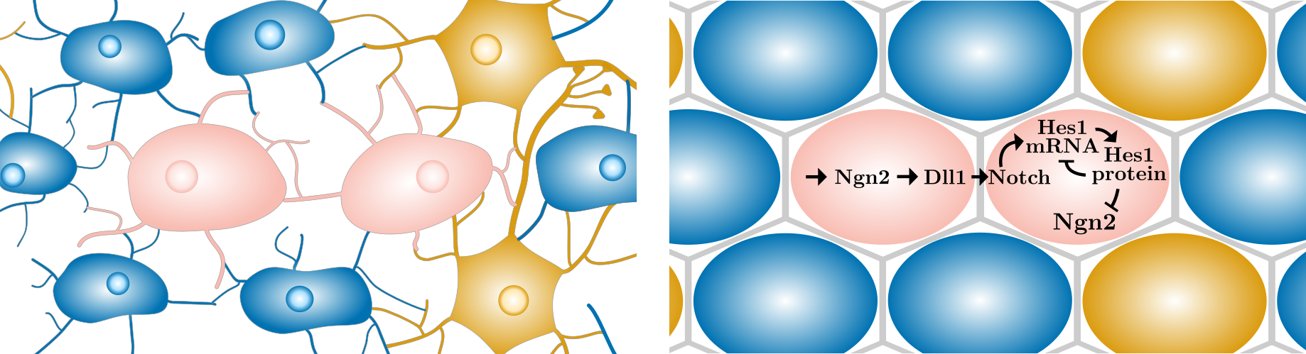
Figure 2.1: Left: Representation of neurons (orange), glial cells (blue) and undifferentiated cells (pink) in a developing brain. Right: Schematics of the Hes1 negative feedback loop in two neighbouring cells. The same interactions occur in every cell throughout the neural progenitor cell population between all neighbouring cells. All arrows ending with an arrowhead denote an activation or creation of a constituent while arrows ending with a vertical line denote a repression. All constituents are also degraded (not shown).

We start with the schematic understanding of the underlying biological processes depicted in Fig. 2.1. Following [35], the main molecules involved in the process of maintaining neural progenitor cells are Neurogenin-2 (Ngn2), Delta-like-1 (Dll1), the Notch receptor as well as Hes1 mRNA and protein which together interact as indicated in the figure. To this end we use the notation

$$D\text{: Dll1, }N\text{: Notch, }M\text{: Hes1 mRNA, }P\text{: Hes1 protein, }n\text{: Ngn2,}$$ (2.1)

for the concentrations of respective constituents in each cell.

Starting in the left pink cell in Fig. 2.1, Ngn2 is constitutively produced and induces the production of Dll1, which in turn is presented on the cell membrane and interacts with the Notch receptor on the surface of the right cell. The internal part of the Notch receptor, the Notch intracellular domain, then interacts with the Hes1 gene promoter to induce the production of Hes1 mRNA which we summarise here as Notch inducing Hes1 mRNA production. However, we are aware that both Dll1 and Notch have a bound/inactive form as well as a free/active form. Both proteins are transmembrane molecules and signalling occurs via direct contact between the proteins [6]. This direct contact renders both proteins unable to function after signalling which becomes relevant during the mathematical modelling process.

Following the biological pathway further, Hes1 protein is then produced from the Hes1 mRNA and successively inhibits the production of new Hes1 mRNA while also repressing the production of the proneural protein Ngn2. Ultimately, this process leads to low levels of Ngn2 and Dll1 in cells which have high levels of Hes1 protein and vice versa. Overall, this results in a stationary “salt and pepper pattern” [35], i.e., with each high level Hes1 protein cell surrounded with cells of low Hes1 protein levels.

2.2 Network ODE Models

Given the schematic understanding of Fig. 2.1, we start by proposing an ODE model to describe the Hes1-Notch GRN within a single cell. In this case we describe Dll1, Notch, Hes1 mRNA, Hes1 protein and Ngn2 as concentrations $[D,N,M,P,n]$, hence extending purely Delta-Notch signalling systems such as [9, 8, 12] to also include the Hes1 negative-feedback dynamics.

We let all molecules be degraded at a rate $\mu_{i}$ with $i\in\{D,N,M,P,n\}$ and capture the inhibition of Hes1 mRNA as well as the repression of the production of the proneural protein Ngn2 using the repressor form of Hill functions of the Hes1 protein [2]. At the same time, the activation or production of each constituent is modelled using $\alpha_{i}$ according to individual dynamics of each molecule. These considerations lead to the system describing the Hes1-Notch GRN in a single cell to be

$$\left.\begin{array}[]{rcl}\dot{D}&=&\alpha_{D}n-\mu_{D}D,\\ \dot{N}&=&\alpha_{N}\langle D_{\text{in}}\rangle-\mu_{N}N,\\ \dot{M}&=&\frac{\alpha_{M}N}{1+(P/K_{M})^{k}}-\mu_{M}M,\\ \dot{P}&=&\alpha_{P}M-\mu_{P}P,\\ \dot{n}&=&\frac{\alpha_{n}}{1+(P/K_{n})^{h}}-\mu_{n}n.\\ \end{array}\right\}$$ (2.7)

Here, $\langle D_{\text{in}}\rangle\mathrel{\mathop{\ordinarycolon}}=\sum_{i}w_{i}D_{i}$ is the average time-dependent Dll1 signal a cell receives from its neighbouring cells $i$ (always normalizing the weights $w_{i}$ to sum to unity). To determine the cell population behaviour, we apply this ODE system on each individual node in a network which represents the connectivity between a population of cells. In this paper we mainly use regular hexagonal grids, however, other grids can easily be treated in the same way.

We propose the parameters as given in Tab. 2.1. Since both the timings of the entire process with oscillations of periods $\sim$ 2–3 hours [18], as well as most parameter values are available for mouse embryonal cell lines, our overall calculations are based on these timings for mouse development. For the degradation rates $\mu_{i}$ we rely on the half-lifes for the associated components except for $D$ and $N$ which, as previously mentioned in §2.1, become inactive upon contact made by signalling due to proteolytic cleavage of the Notch receptor. Thus, we assume that $80\%$ of both proteins are used while $20\%$ are free and can be degraded, c.f. Tab. 2.1. One element deciding system behaviour is the choice of the Hill coefficients $k$ and $h$. We require both $k,h\in\mathbb{N}^{+}$ and choose $k=1$ and $h=4$ as these are the minimum values which we have found are necessary to realistically capture oscillations. Similarly, we choose $K_{M}$ and $K_{n}$ to fit overall system behaviour and do not consider perturbations for these values as the system is underdetermined. Given degradation rates and with fixed Hill functions, our activation rates $\alpha_{i}$ follow by fitting to the relative amounts of each component as found in [21]. The uncertainty of these activation rates are found by a straightforward Monte Carlo approach, using the independent perturbations in Tab. 2.1 and assuming $5\%$ noise for the concentrations. For more information about this, see Appendix A. The resulting typical dynamics of the model are shown in Fig. 2.2.

Parameter	Value (68% Confidence Interval)	Reference
$\alpha_{D}$	$0.018\ (0.016,0.021)$ [/min]	This paper
$\alpha_{N}$	$6.0\ (5.3,6.7)$ [/min]
$\alpha_{M}$	$0.017\ (0.016,0.019)$ [/min]
$\alpha_{P}$	$0.14\ (0.12,0.16)$ [/min]
$\alpha_{n}$	$0.0049\ (0.0043,0.0054)$ [$\mu M$/min]
$\mu_{D}$	$\log 2/50\times 5\ \log(2)/(45.3,55.2)\times 5$ [/min]	Dll1 half-life in mice [36]
$\mu_{N}$	$\log 2/40\times 5\ \log(2)/(36.2,44.2)\times 5$ [/min]	Notch1 half-life in humans [1]
$\mu_{M}$	$\log 2/24.1\ \log 2/(22.4,25.8)$ [/min]	Hes1 protein half-life in mice [18]
$\mu_{P}$	$\log 2/22.3\ \log 2/(19.2,25.4)$ [/min]	Hes1 mRNA half-life in mice [18]
$\mu_{n}$	$\log 2/21.9\ \log 2/(19.7,24.1)$ [/min]	Ngn2 half-life in Xenopus [41]
$K_{M}$	$\equiv 0.050$ [$\mu M$]	This paper
$K_{n}$	$\equiv 0.030$ [$\mu M$]
$k$	$\equiv 1$	This paper
$h$	$\equiv 4$

Table 2.1: Parameters for (2.7). Values of $\alpha_{i}$ are chosen to give the desired behaviour of constituents relative to each other [21], while $\mu_{i}$ values are based on the half-lives of the components of the GRN, mostly in mice. For $D$ and $N$, specifically, we make the modelling assumption that $80\%$ of each is bound, thus, leading to the multiplication by the factor $5$. Where values are available with error estimates we use those, while for $\alpha_{i}$ we fit them to all other perturbed parameters, and for $\mu_{D}$ and $\mu_{N}$ we assume an ad hoc $\pm 10\%$ uncertainty since the value for $\mu_{N}$ is more uncertain (a higher range of values including an NICD half-life of $\sim 180$ min [22] has been reported). To achieve the behaviour we desire, the value from [1] was used for this parameter.

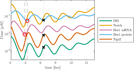
Figure 2.2: Dynamics averaged over all cells on a $20$-by-$20$ grid of hexagonal cells when starting from random initial data. The two dashed vertical lines indicate the offset between Hes1 mRNA and Hes1 protein expression levels which has been shown previously in [18]. The offset between the Hes1 mRNA and Hes1 protein oscillations between the two markers as shown is approximately $30$ minutes. The vertical dotted line shows that we approximately capture the inverse oscillations between the Hes1 protein, and Dll1 and Ngn2 [35].

For improved ability to analyse the system, we assume quasi-steady states for three of the five states to find a reduced ODE system. Depending on the reduction we choose, we find either equations of type 1,

$$\left.\begin{array}[]{rclcl}\dot{x}&=&\frac{\langle y_{\text{in}}\rangle}{a+x^{k}}-x&=\mathrel{\mathop{\ordinarycolon}}&\langle y_{\text{in}}\rangle f(x)-x\\ \dot{y}&=&v\left(\frac{1}{1+bx^{h}}-y\right)&=\mathrel{\mathop{\ordinarycolon}}&v\left(g(x)-y\right)\end{array}\right\},$$ (2.10)

or of types 2 and 3, respectively,

$$\left.\begin{array}[]{rcl}\dot{x}&=&yf(x)-x\\ \dot{y}&=&v\left(\langle g(x_{\text{in}})\rangle-y\right)\end{array}\right\},\qquad\left.\begin{array}[]{rcl}\dot{x}&=&\langle g(y_{\text{in}})\rangle f(y)-x\\ \dot{y}&=&v\left(x-y\right)\end{array}\right\},$$ (2.15)

where $f$ and $g$ are as for type 1 and where $\langle g(x_{\text{in}})\rangle=\sum_{i}w_{i}g(x_{i})$ is the average of $g(x_{i})$ across the neighbour cells $i$. Overall, there are $10$ possible ways to reduce the original system (2.7) to a two-dimensional system by making quasi-steady state assumptions. However, three possible options, those where neither $x$ nor $y$ represent $M$ or $P$, are not readily reducible since the reduction involves solving Hill equations. This leaves seven possible alternatives (four of type 1, two of type 2 and one of type 3) capturing the steady state behaviour of the original system (2.7). The different alternatives are summarised in Tab. 2.2, and a typical derivation can be found in Appendix B. For comparision, the behaviour of both the full model (2.7) and the best fit reduced model (2.10) are shown in Fig. 2.3. To note about the reduced models in (2.10) and (2.15) is that they all end up with the same parameters $a$ and $b$, cf. Tab. 2.2, while $v$ varies such that all three reduced model types behave similarly except for the timing of fate decision which is determined by $v$.

To further simplify analysis, at points we use a scalar version of our model. To reach this, we make the further assumption that $\dot{y}=0$ in either of the two-dimensional models (2.10)–(2.15). This reduces all three types into

$$\dot{x}=\langle g(x_{\text{in}})\rangle f(x)-x.$$ (2.16)

Our reduced models (2.10)–(2.15) are remindful of the Delta-Notch model from [9],

$$\left.\begin{array}[]{rclcl}\dot{x}&=&\frac{\langle y_{\text{in}}\rangle^{k}}{a+\langle y_{\text{in}}\rangle^{k}}-x&=\mathrel{\mathop{\ordinarycolon}}&F(\langle y_{\text{in}}\rangle)-x\\ \dot{y}&=&v\left(\frac{1}{1+bx^{h}}-y\right)&=\mathrel{\mathop{\ordinarycolon}}&v\left(G(x)-y\right)\end{array}\right\},$$ (2.19)

where $x$ describes Notch, $y$ describes Delta, and $\langle y_{\text{in}}\rangle$ is the average incoming Delta from the neighbours on the grid. While our models (2.10) and (2.15) show differences in the form of $f(x)$, the order of averaging and Hill functions, the values of the Hill coefficients $k$ and $h$, as well as where the model links the incoming signal compared to the Collier model (2.19), we can use an analysis similar to the one proposed in [9] to investigate the behaviour of our system further.

type	$x$	$y$	$v$
1	$\mathbf{M}$	$\mathbf{n}$	$\mathbf{1.096\ (0.975,1.280)}$
1	$P$	$n$	$1.014\ (0.851,1.100)$
1	$M$	$D$	$2.410\ (2.111,2.740)$
1	$P$	$D$	$2.230\ (1.800,2.627)$
2	$M$	$N$	$3.013\ (2.712,3.401)$
2	$P$	$N$	$2.788\ (2.298,3.280)$
3	$M$	$P$	$1.081\ (0.936,1.305)$

Table 2.2: The seven alternative ways to reduce the original system (2.7) to (2.10) or (2.15) via quasi-steady state assumptions and the resulting effective parameter $v$. The parameters $a$ and $b$ are $0.083\ (0.071,0.094)$ and $1.652\times 10^{5}\ (0.807,3.217)\times 10^{5}$ for all alternatives ($68\%$ confidence intervals). The version displayed in Fig. 2.3 is indicated in bold.

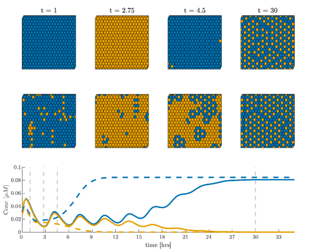
Figure 2.3: Top row: spatial dynamics of Hes1 mRNA in our proposed grid ODE model (2.7) where blue cells are above the mean concentration before fate decision and orange cells are below this threshold. Middle: Hes1 mRNA in the reduced model (2.10) on the same grid. Bottom: the average Hes1 mRNA (solid line: full ODE model; dashed line: reduced model) over time with blue and orange denoting high and low expression, respectively. The horizontal lines denote the times at which the spatial dynamics are shown in the top and middle rows. Note that by our parameterisation, we find our results in concentrations.

2.3 Spatial Stochastic Reaction-transport Model

To take intra-cellular noise into account we also consider a mesoscopic stochastic version of the grid ODE (2.7) as follows. We represent the individual cells as nodes in a network with connectivity given by an underlying mesh discretization. Consider a single cell first, with time-dependent state vector $X(t)\in\mathbf{Z}_{+}^{d}$ counting at time $t$ the number of constitutents (or species) in each of $d$ compartments. We may generally prescribe $R$ Markovian reactions in the form of Poissonian state transitions $X\mapsto X+\mathbb{N}_{r}$ by

$$\mathbf{P}\left[X(t+dt)=x+\mathbb{N}_{r}|\;X(t)=x\right] =w_{r}(x)\,dt+o(dt),$$ (2.20)

for $r=1\ldots R$ with $w_{r}(x)$ the $r$th transition intensity (or propensity), and $\mathbb{N}\in\mathbf{Z}^{d\times R}$ the stoichiometric matrix. The evolution of the $i$th species can then be described by the Poisson representation [33]

$$X_{i}(t) =X_{i}(0)+\sum_{r=1}^{R}\mathbb{N}_{ri}\Pi_{r}\left(\int_{0}^{t}w_{r}(X(s))\,ds\right),$$ (2.21)

with unit-rate and independent Poisson processes $(\Pi_{r})_{r=1}^{R}$.

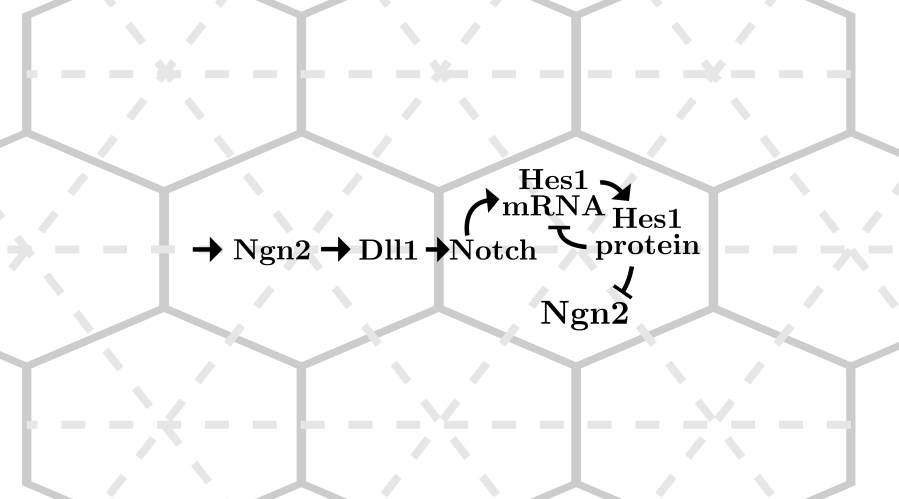
Figure 2.4: The schematics as implemented on a hexagonal grid (solid lines) using the RDME model. The dashed lines show the triangulation on which the hexagonal grid is built in the URDME framework.

In the present case we identify the following reactions:

$$\left.\begin{array}[]{rcl}n&\xrightarrow{\alpha_{D}n}&n+D\\ N&\xrightarrow{\alpha_{M}N/(1+P/(K_{M}V)^{k})}&N+M\\ M&\xrightarrow{\alpha_{P}M}&M+P\\ \emptyset&\xrightarrow{\alpha_{n}V/(1+P/(K_{n}V)^{h})}&n\end{array}\right\}\qquad\left.\begin{array}[]{rcl}D&\xrightarrow{\mu_{D}D}&\emptyset\\ N&\xrightarrow{\mu_{N}N}&\emptyset\\ M&\xrightarrow{\mu_{M}M}&\emptyset\\ P&\xrightarrow{\mu_{P}P}&\emptyset\\ n&\xrightarrow{\mu_{n}n}&\emptyset\end{array}\right\}$$ (2.31)

where $V$ is the volume of each voxel. The production of Notch, as initiated by the Dll1 signal, is yet to be described.

We next consider a population of cells in $K$ nodes or voxels $(V_{k})_{k=1}^{K}$ and a time-dependent state $X\in\mathbf{Z}_{+}^{d\times K}$, with $X_{ik}(t)$ the number of constituents of the $i$th species in the $k$th voxel. The general dynamics (2.21) now becomes

$$X_{ik}(t)=X_{ik}(0) +\sum_{r=1}^{R}\mathbb{N}_{ri}\Pi_{rk}\left(\int_{0}^{t}V_{k}u_{r}(V_{k}^{-1}X_{\cdot,k}(s))\,ds\right)$$ (2.32)

$$-\sum_{k=1}^{J}\Pi_{ijkl}^{\prime}\left(\int_{0}^{t}q_{ijkl}X_{ik}(s)\,ds\right)+\sum_{k=1}^{J}\Pi_{jilk}^{\prime}\left(\int_{0}^{t}q_{jilk}X_{jl}(s)\,ds\right),$$

where $q_{ijkl}$ is the rate per unit of time for species $i$ in the $k$th voxel to transfer into species $j$ in the $l$th voxel, and where $(\Pi_{\cdot},\Pi^{\prime}_{\cdot})$ is an appropriately extended set of independent unit-rate Poisson processes. This general linear transfer process is not standard as it allows for species to change their type while transporting, but it is appropriate here since it is exactly this effect we are interested in. Note also that in (2.32), the propensities $(u_{r})$ are independent of the voxel volume $V_{k}$. Using this formalism we may augment (2.31) with

$$\left.\begin{array}[]{rrl}D&\xrightarrow{\alpha_{N}D}&D+D^{\text{in}}\\ D_{k}^{\text{in}}&\xrightarrow{\alpha_{N}q_{kl}D_{k}^{\text{in}}}&N_{l}\end{array}\right\}$$ (2.35)

that is, a Dll1 signal in voxel $k$ sequentially transforms into a diffusing pseudo species $D^{\text{in}}$, which then diffuses into a Notch signal in voxel $l$ at rate $\alpha_{N}q_{kl}$, where $q_{kl}$ is the proportion of Dll1 used for the signal between these two voxels (for example, $q_{kl}\equiv 1/6$ on a hexagonal mesh with $k$ and $l$ neighbouring voxels).

The model so described can readily be implemented across a given triangulation of space using URDME [4] and simulated using the supported NSM-solver with a triangulation as illustrated in Fig. 2.4. Sample simulations are reported in Fig. 2.5.

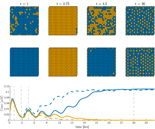
Figure 2.5: Top row: spatial dynamics of Hes1 mRNA in our RDME model (2.31) and (2.35) choosing the volume of each voxel to be $1\mu m^{3}$, representing a rather high noise levels, and using the same colour scheme as in Fig. 2.3. Middle: Hes1 mRNA in the RDME model with voxel volume $50\mu m^{3}$, i.e., less levels of noise. Bottom: the average Hes1 mRNA at low volume, $1\mu m^{3}$, (dashed line) and high volume, $50\mu m^{3}$, (solid line) over time where the horizontal lines denote the times at which the spatial dynamics are shown in the top and middle rows. Blue and orange, again, denote cells with high and low expression. Based on a mouse embryonal stem cell volume of approximately $50\mu m^{3}$ [size based on [31, 42] assuming spherical cells] and a mean number of $8104$ molecules per cell [19], we find our results in $\mu M$.

3 Analysis and Results

We next analyse the properties of the system (2.7). Existence and qualitative behaviour of fate decision in a two-cell 1D periodic system in the reduced model (2.10)–(2.16) is investigated in §3.1 and in the full model (2.7) in §3.2. We then examine the behaviour of the system (2.10) on a regular hexagonal grid in §3.3, and we finally quantitatively compare the patterning differences between the ODE (2.7) and RDME models (2.31)–(2.35) in §3.4.

3.1 The Reduced Stationary Solutions

At stationary solutions to (2.7), the quasi-stationary arguments used to arrive at the reduced systems (2.10)–(2.16) are valid and so we target these models initially. We first consider the homogeneous steady state where, by “homogeneous” we simply mean that all cells have identical states. We pick the scalar reduced model (2.16), i.e.,

$$\dot{x} =g(\langle x_{\text{in}}\rangle)f(x)-x,$$ (3.1)

where $f,g$ are as in (2.10). Looking for a homogeneous steady state where $\langle x_{\text{in}}\rangle=x$, we define $\varphi(x)\mathrel{\mathop{\ordinarycolon}}=g(x)f(x)$ and equivalently search for fixed points satisfying $\varphi(x)=x$. Since $0<\varphi(0)$, $\varphi(1)<1$, and since $f$, $g$, and, hence, also $\varphi$ are all decreasing functions there is a unique root $\bar{x}_{0}$ in $(0,1)$, cf. Fig. 3.1. In conclusion,

Proposition 3.1.

There is a unique stationary point $\bar{x}_{0}\in(0,1)$ for the homogeneous problem (3.1). By extension this unique solution also applies to the homogeneous version of the full system (2.7).

Since we want to show that our system undergoes fate decision into a non-homogeneous solution, we next investigate the stability properties of the homogeneous steady state in the simplest one-dimensional setting consisting of two cells with a periodic boundary condition.

Proposition 3.2.

The homogeneous stationary solution in the reduced system (2.10) is unstable in a system with two cells under a periodic boundary condition if and only if

$$f(\bar{x}_{0})g^{\prime}(\bar{x}_{0})-f^{\prime}(\bar{x}_{0})g(\bar{x}_{0}) <-1,$$ (3.2)

for $\bar{x}_{0}$ the homogeneous stationary solution.

Proof.

The two-cell periodic system reads

$$\left.\begin{aligned} \dot{x_{1}}&=g(x_{2})f(x_{1})-x_{1}\\ \dot{x_{2}}&=g(x_{1})f(x_{2})-x_{2}\end{aligned}\right\}.$$ (3.3)

We assume small perturbations about the homogeneous steady state and introduce the change of variables

$$\sigma =\frac{x_{1}+x_{2}}{2},\quad \delta =\frac{x_{1}-x_{2}}{2},$$ (3.4)

where we consider the perturbation $\delta$ small. Expanding the system around the homogeneous stationary solution, the equations decouple and we find the governing equation

$$\dot{\delta}=\left(f^{\prime}(\sigma)g(\sigma)-f(\sigma)g^{\prime}(\sigma)-1\right)\delta.$$ (3.5)

Letting $\sigma=\bar{x}_{0}$ we obtain condition (3.2). ∎

This result holds for parameter $(a,b)>0$ which holds for all reductions to any of the reduced systems. That the previous result remains true for the full system (2.7) is more involved to show so we defer this to the next section §3.2.

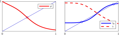
Figure 3.1: Fix point arguments. Left: the unique homogeneous stationary state is the fix point $\bar{x}_{0}=\varphi(\bar{x}_{0})$. Right: if $\gamma_{2}^{\prime}(\bar{x}_{0})>1$, then there are cyclic (non-homogeneous) solutions $\bar{x}_{1}<\bar{x}_{0}<\bar{x}_{2}$.

We next consider the existence of a non-homogeneous steady state. We again assume a 2-cell periodic set up and thus look for stationary solutions to (3.3).

Proposition 3.3.

Under condition (3.2) there exists a non-homogeneous stationary state for the 2-cell periodic problem (3.3). By extension this solution also applies to the corresponding periodic version of (2.7).

Proof.

From (3.3) we have the stationary relation

$$h(x_{1})\mathrel{\mathop{\ordinarycolon}}=\frac{x_{1}}{f(x_{1})}=g(x_{2}),\mbox{ or }x_{1}=h^{-1}(g(x_{2}))=\mathrel{\mathop{\ordinarycolon}}\gamma(x_{2}).$$

For positive arguments, the function $h$ is increasing, hence $h^{-1}$ is increasing too, and with $g$ decreasing, $\gamma$ is therefore a decreasing function. One readily shows that $\gamma(0)>0$ and $\gamma(1)<1$ which together forms a second proof of the existence of the unique fix point $\bar{x}_{0}$ for the homogeneous stationary state. However, we are rather interested in cyclic solutions, i.e., for which $x=(\gamma\circ\gamma)(x)=\mathrel{\mathop{\ordinarycolon}}\gamma_{2}(x)$, since these correspond to alternating (patterned) solutions in the 2-cell problem. It is easy to see that $\gamma_{2}(0)>0$ and $\gamma_{2}(1)<1$ and since $\gamma_{2}(\bar{x}_{0})=\bar{x}_{0}$ we find two additional solutions $\bar{x}_{1}<\bar{x}_{0}<\bar{x}_{2}$ under the condition that $\gamma_{2}^{\prime}(\bar{x}_{0})>1$, cf. Fig. 3.1 (right). We get

$$\frac{d}{d\xi}\gamma(\gamma(\xi))|_{\xi=\bar{x}_{0}}>1 \iff\gamma^{\prime}(\gamma(\xi))\gamma^{\prime}(\xi)|_{\xi=\bar{x}_{0}}=\gamma^{\prime}(\bar{x}_{0})^{2}>1\iff\gamma^{\prime}(\bar{x}_{0})<-1.$$ (3.6)

We find via implicit differentiation and using $\bar{x}_{0}=\gamma(\bar{x}_{0})$ that

$$\gamma^{\prime}(\bar{x}_{0}) =\frac{g^{\prime}(\bar{x}_{0})}{h^{\prime}\left(\gamma(\bar{x}_{0})\right)}=\frac{f(\bar{x}_{0})g^{\prime}(\bar{x}_{0})}{1-\bar{x}_{0}\,f^{\prime}(\bar{x}_{0})/f(\bar{x}_{0})}=\frac{f(\bar{x}_{0})g^{\prime}(\bar{x}_{0})}{1-g(\bar{x}_{0})f^{\prime}(\bar{x}_{0})},$$

revealing that, in fact, (3.6) is equivalent to condition (3.2). ∎

One cannot rule out the existence of more than one set of non-homogeneous solutions. To select a specific one, we pick the one pair $(\bar{x}_{1},\bar{x}_{2})$ which is the furthest away from $\bar{x}_{0}$. By inspection this solution also satisfies

$$\gamma_{2}^{\prime}(\bar{x}_{1})=\gamma_{2}^{\prime}(\bar{x}_{2})=\gamma^{\prime}(\bar{x}_{1})\gamma^{\prime}(\bar{x}_{2})<1,$$ (3.7)

cf. Fig. 3.1 (right). Interestingly, this property guarantees stability of this solution as we next demonstrate.

Proposition 3.4.

The non-homogeneous solution of Proposition 3.3 is stable whenever it exists.

Proof.

The Jacobian around the non-homogeneous solution has the characteristic polynomial

$$p(\lambda) =(\lambda-f^{\prime}_{1}g_{2}+1)(\lambda-f^{\prime}_{2}g_{1}+1)-f_{1}f_{2}g_{1}^{\prime}g_{2}^{\prime},$$

where $f_{1}=f(\bar{x}_{1})$ and similarly for $f^{\prime}_{1}$, $g_{1}$, $g^{\prime}_{2}$, etc. By inspection all coefficients are positive except for the 0th order term. By Descarte’s rule of sign there is a positive real eigenvalue if an only if this term is negative, that is, the non-homogeneous stationary solution is stable if and only if

$$0 <f^{\prime}_{1}f^{\prime}_{2}g_{1}g_{2}-f_{1}f_{2}g_{1}^{\prime}g_{2}^{\prime}-f^{\prime}_{1}g_{2}-f^{\prime}_{2}g_{1}+1.$$ (3.8)

For the function $\gamma$ introduced in the proof of Proposition 3.3, we have

$$\gamma^{\prime}(\bar{x}_{1}) =\frac{g^{\prime}_{1}}{h^{\prime}\left(\gamma(\bar{x}_{1})\right)}=\frac{f_{2}g^{\prime}_{1}}{1-\bar{x}_{2}\,f^{\prime}_{2}/f_{2}}=\frac{f_{2}g^{\prime}_{1}}{1-f^{\prime}_{2}g_{1}},$$

and similarly for $\gamma^{\prime}(\bar{x}_{2})$. Hence, from rearranging the property (3.7) we find

$$(1-f^{\prime}_{2}g_{1})(1-f^{\prime}_{1}g_{2}) >f_{1}f_{2}g^{\prime}_{1}g^{\prime}_{2},$$

which is equivalent to condition (3.8). ∎

So far we have shown that there always exists a unique homogeneous stationary solution. For the 2-cell periodic problem and under condition (3.2), this solution is unstable and there is then another non-homogeneous solution which is stable. Fig. 3.2 illustrates this behaviour along a certain selected path in parameter space for the full model (2.7). We next proceed to show that as suggested by this graphic, the results indeed hold for the full model as well.

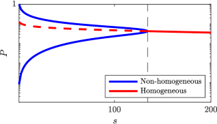
Figure 3.2: The non-homogeneous and homogeneous stationary states of $P$ (log-scale), respectively, as a function of a scaling $s$, which acts upon the parameter $\alpha_{N}$, by scaling $\alpha_{N}\mapsto s^{-1}\alpha_{N}$. The homogeneous solution always exists, but is unstable to the left of the dashed line which indicates the smallest value of $s$ for which (3.2) and (3.19) are true.

3.2 Extension to the Full Model

To understand in what way the reduced models capture the stability properties of the full model, we need to describe how they are related at sufficient detail. Let a general ODE have the form $\dot{x}=F(x)$ and assume that the state has been split according to $x=[y;\;z]$, that is,

$$\begin{bmatrix}\dot{y}\\ \dot{z}\end{bmatrix} =\begin{bmatrix}F_{y}(y,z)\\ F_{z}(y,z)\end{bmatrix}.$$ (3.9)

The reduced model for $z$ is obtained by assuming that $\dot{y}\approx 0$ and such that, given $z$, $y$ can be uniquely solved for

$$0 =F_{y}(y,z)\iff y=G(z).$$ (3.10)

The reduced model is then simply

$$\dot{z} =F_{z}(G(z),z),$$ (3.11)

and the reduced model’s Jacobian is given by

$$J_{z} =\partial_{y}F_{z}G^{\prime}(z)+\partial_{z}F_{z}=-\partial_{y}F_{z}[\partial_{y}F_{y}]^{-1}\partial_{z}F_{y}+\partial_{z}F_{z}.$$ (3.12)

By contrast, the full Jacobian reads

$$J =\begin{bmatrix}\partial_{y}F_{y}&\partial_{z}F_{y}\\ \partial_{y}F_{z}&\partial_{z}F_{z}\end{bmatrix},$$ (3.13)

and by a block decomposition [20] the determinant is given by

$$\det(J) =\det(\partial_{y}F_{y})\times\det\left(\partial_{z}F_{z}-\partial_{y}F_{z}[\partial_{y}F_{y}]^{-1}\partial_{z}F_{y}\right).$$ (3.14)

In general, both Jacobians $J$ and $J_{z}$ depend on a parameter vector $\theta$, say, such that we can write $J=J(\theta)$ and equivalently for $J_{z}$. Since the determinant of the negative Jacobian is the 0th order term of the characteristic polynomial, we formulate the following lemma by comparing (3.12) and (3.14):

Lemma 3.5.

Let $p_{x}(\lambda)\equiv\det(\lambda I-J)$ be the characteristic polynomial for the full Jacobian and equivalently define $p_{z}(\lambda)\equiv\det(\lambda I-J_{z})$. Suppose that for some parameter $\theta$, all coefficients are positive except for possibly the 0th order term $p_{x}(0)$. Suppose also that the order reduction is definite in the sense that $\partial_{y}F_{y}$ is either positive or negative definite for all considered parameters $\theta$. Then, as a function of $\theta$, $p_{x}(0)$ switches sign simultaneously with $p_{z}(0)$ and in fact, $p_{x}(0)=\det(-\partial_{y}F_{y})\times p_{z}(0)$.

The main use of the lemma is in conjunction with Descarte’s rule of sign as it allows one to conclude that the spectrum of $J$ switches from stable to unstable at points for which $J_{z}$ is singular. The expressions for these points are typically simpler to obtain than for the full system. However, one still has to show that the full characteristic polynomial has positive terms of higher order than 0.

Proposition 3.6.

Let $P_{0}$ be the homogeneous stationary solution for state $P$ of the full model (2.7). This solution is unstable for the 2-cell periodic problem if and only if

$$-\frac{h(P_{0}/K_{n})^{h}}{1+(P_{0}/K_{n})^{h}}+kP_{0}(P_{0}/K_{M})^{k}(1+(P_{0}/K_{n})^{h})\times R <-1,$$ (3.15)

where $R\equiv\prod_{i}\alpha_{i}/\mu_{i}$, $i\in\{D,N,M,P,n\}$.

Under the reduction (2.10) (cf. §B) we have that

$$a =(K_{M}/R)^{k/(k+1)},$$ (3.16)

$$b =\left(K_{M}^{k/(k+1)}/K_{n}\times R^{1/(k+1)}\right)^{h},$$ (3.17)

$$P_{0} =R^{1/(k+1)}\times(\alpha_{P}/\mu_{P})^{2k/(k+1)}K_{M}^{-k/(k+1)}\times\bar{x}_{0},$$ (3.18)

where we recall that $\bar{x}_{0}\in(0,1)$ is the homogeneous stationary solution for the reduced model as in Proposition 3.1.

Proof.

After the same type of change of variables as in (3.4) and linearising around small perturbations, we obtain a relatively sparse linear time-dependent system. The characteristic polynomial $p(\lambda)$ can therefore be obtained via iterated cofactor expansions. Writing $f_{k}(x)=1/(1+x^{k})$ and similarly for $f_{h}$, we find

$$p(\lambda) =(\lambda+\mu_{D})(\lambda+\mu_{N})(\lambda+\mu_{n})\left[(\lambda+\mu_{M})(\lambda+\mu_{P})-N_{0}\alpha_{M}\alpha_{P}f^{\prime}_{k}(P_{0}/K_{M})/K_{M}\right]$$

$$\hphantom{=}+\alpha_{D}\alpha_{N}\alpha_{M}\alpha_{P}\alpha_{n}f^{\prime}_{h}(P_{0}/K_{n})f_{k}(P_{0}/K_{M})/K_{n}.$$

By inspection all coefficients of the polynomial are positive except for possibly the constant term. We verify that $\det(-\partial_{y}F_{y})=\mu_{N}\mu_{M}\mu_{D}\mu_{n}>0$ in the notation of Lemma 3.5 and so it follows that the stability condition (3.2) is preserved by the state reduction. Using the relations (3.16)–(3.18) and the fix point relation $\bar{x}_{0}=f(\bar{x}_{0})g(\bar{x}_{0})$ we find that (3.2) is equivalent to (3.19). ∎

It remains to show that the non-homogeneous solution also shares its stability properties with the reduced model.

Proposition 3.7.

The non-homogeneous solution of Proposition 3.3 is stable for the full model (2.7) whenever it exists.

Proof.

This time we linearise around the non-homogeneous solution and obtain a 10-by-10 Jacobian. Luckily the Jacobian is rather sparse such that its characteristic polynomial can be expanded into

$$p(\lambda) =(\lambda+\mu_{D})^{2}(\lambda+\mu_{N})^{2}(\lambda+\mu_{n})^{2}\times$$

$$\phantom{=}\left[(\lambda+\mu_{M})(\lambda+\mu_{P})-N_{1}\alpha_{M}\alpha_{P}f^{\prime}_{k}(P_{1}/K_{M})/K_{M}\right]\times$$

$$\phantom{=}\left[(\lambda+\mu_{M})(\lambda+\mu_{P})-N_{2}\alpha_{M}\alpha_{P}f^{\prime}_{k}(P_{2}/K_{M})/K_{M}\right]$$

$$\phantom{=}-(\alpha_{D}\alpha_{N}\alpha_{M}\alpha_{P}\alpha_{n}/K_{n})^{2}f^{\prime}_{h}(P_{1}/K_{n})f^{\prime}_{h}(P_{2}/K_{n})f_{k}(P_{1}/K_{M})f_{k}(P_{2}/K_{M}).$$

All coefficients of the polynomial are positive except for possibly the constant term. The reduction map is verified to be positive definite and so we conclude that the stability condition (3.19) again controls the stability also of the non-homogeneous solution. ∎

3.3 Patterning on Regular Hexagonal Tilings

Next we are interested in analysing the patterning that occurs when a non-homogeneous steady state is reached. From a biological perspective, a “random” pattern or a chaotic non-stationary behaviour is implausible in a highly regulated pathway. As we have shown in Propositions 3.2 and 3.6, the homogeneous steady state is unstable in both the reduced and the full models under conditions (3.2) and (3.19), assuming a two-cell system with periodic couplings. When the homogeneous steady state is unstable, the heterogeneous steady state exists and is stable (Propositions 3.3, 3.4, 3.7). Again, this holds for the simple case of a two-cell system with periodic couplings, but we are nevertheless led to believe that a regular periodic pattern will eventually result from the model.

On a regular hexagonal tiling, there are a multitude of regularly periodic patterns that can occur, yet not every such periodic pattern is uniform or vertex-transitive. In the case of the non-uniform pattern illustrated in Fig. 3.3, for example, we require two ‘sub-types’ of white cells: those that border black cells and those that do not. We argue that for symmetry reasons, assuming a vertex-transitive pattern is a reasonable assumption for further investigations of our model. There exist three such uniform colourings on a regular hexagonal tiling [15], see Fig. 3.4, one of which describes the homogeneous case.

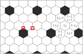
Figure 3.3: A regularly periodic pattern on a hexagonal grid with period $3$ in each lattice direction. The labelling scheme shown follows [9]. The red squares highlight two vertices which make the pattern non-transitive: the left borders 2 white and one black cell, while the right borders 3 white cells.

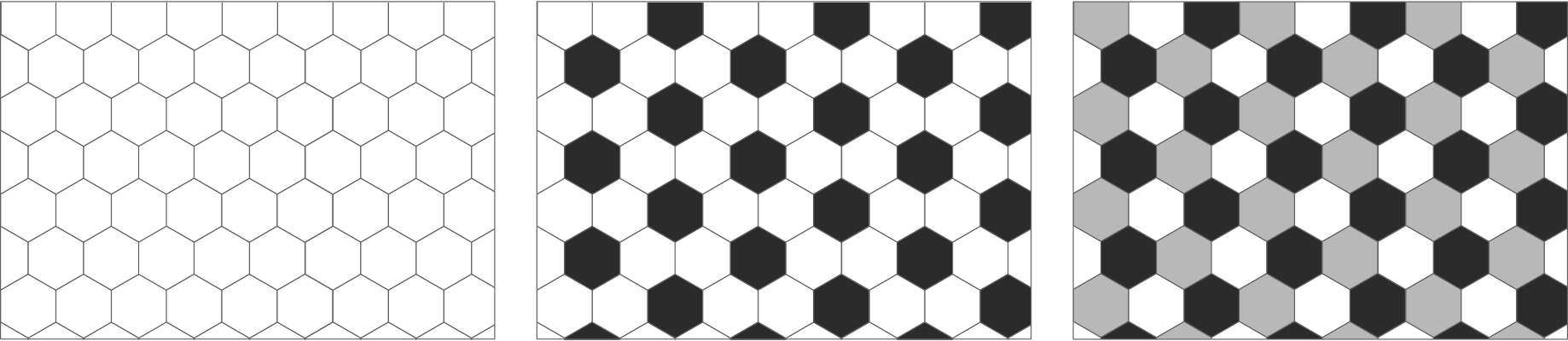
Figure 3.4: The three patterns on a regular hexagonal tiling which show vertex transitive behaviour, i.e., every vertex has the same neighbours. Note that the right pattern is identical to the middle pattern if two colours are the same.

Proposition 3.8.

Under periodic boundary conditions the homogeneous steady state of the reduced system (2.16) is conditionally unstable in both one and two dimensions. Conditions for instablity are the previous (3.2), while in 2D the condition is found in (3.19) below.

Proof.

On a one-dimensional lattice with $j=1,2,\ldots,N$, we find from (2.16) the governing equations

$$\dot{x}_{j} =\frac{g(x_{j-1})+g(x_{j+1})}{2}f(x_{j})-x_{j}.$$

Linearising around the homogeneous solution and writing $$x_{j}=\bar{x}_{0}+\delta_{j}$$ we find

$$\dot{\delta}_{j} =g^{\prime}f\frac{\delta_{j-1}+\delta_{j+1}}{2}+gf^{\prime}\delta_{j}-\delta_{j}.$$

Inserting the Fourier representation

$$\delta_{j} =\sum_{s=1}^{N}\xi_{s}\exp\left(\frac{2\pi isj}{N}\right),$$

we get

$$\dot{\xi}_{s} =\left(g^{\prime}f\cos\left(\frac{2\pi}{N}s\right)+gf^{\prime}-1\right)\xi_{s}.$$

By inspection the most unstable case occurs for $s/N=1/2$ which is then equivalent to condition (3.2).

On a two-dimensional, regular hexagonal lattice with $j=1,2,\ldots,M$ and $l=1,2,\ldots,N$, we similarly find the governing equations

$$\dot{x}_{lj} =\frac{\sum g(x_{l\pm 1,j\pm 1})}{6}f(x_{lj})-x_{lj},$$

where the sum involves the 6 lattice neighbours, cf. Fig. 3.3. Linearising around the homogeneous solution, we find

$$\dot{\delta}_{lj} =g^{\prime}f\frac{\sum\delta_{l\pm 1,j\pm 1}}{6}+gf^{\prime}\delta_{lj}-\delta_{lj}.$$

Again making use of the Fourier representation,

$$\delta_{lj} =\sum_{r=1}^{M}\sum_{s=1}^{N}\xi_{rs}\exp\left(\frac{2\pi irl}{M}+\frac{2\pi isj}{N}\right),$$

this becomes

$$\dot{\xi}_{rs} =\left(g^{\prime}fA+gf^{\prime}-1\right)\xi_{rs},$$

where

$$3A \equiv\cos\left(\frac{2\pi}{N}s\right)+\cos\left(\frac{2\pi}{M}r\right)+\cos\left(\frac{2\pi}{N}s+\frac{2\pi}{M}r\right).$$

The most unstable case occurs for $s=r=N/3$, assuming $N=M$ and divisibility by 3. The implied condition for instability is then

$$f(\bar{x}_{0})g^{\prime}(\bar{x}_{0})/2-f^{\prime}(\bar{x}_{0})g(\bar{x}_{0}) <-1.$$ (3.19)

∎

It is tempting to draw the conclusion that the corresponding unstable frequency is also the resulting pattern: with period $N/3$ this would indeed imply the middle pattern in Fig. 3.4 which is also what we observe from numerical experiments. However, the analysis only reveals the most unstable modes around the homogeneous solution and does not predict the eventual end-fate.

From numerical experiments we consistently find that the typical stationary pattern generally matches that of Fig. 3.4 (middle), with black/white corresponding to, respectively, low/high Hes1 protein concentrations. Since the stationary state only consists of two distinct states it seems intuitive to attempt to analyze the situation by looking at the two-cell model in two dimensions coupled according to

$$W_{2} =\begin{bmatrix}0&1\\ 1/2&1/2\end{bmatrix},$$ (3.20)

that is, we consider the generic coupled model

$$\dot{x}_{i} =\sum_{j}W_{ij}g(x_{j})\times f(x_{i})-x_{i},$$ (3.21)

for $i=1,2$ and $W=W_{2}$. However, this immediate two-dimensional extension of the two-cell periodic one-dimensional case gives incorrect results. This case supports non-homogeneous stable solutions which are close to the homogeneous one but which are never observed in larger simulations.

A better generalisation is rather three cells, that is, the smallest integer multiple of three as suggested by the previous Fourier analysis. Namely, we take the generic model (3.21) with $W=W_{3}$,

$$W_{3} =\begin{bmatrix}0&1/2&1/2\\ 1/2&0&1/2\\ 1/2&1/2&0\end{bmatrix},$$ (3.22)

and $i=1,\ldots,3$. Consider first the labels “low/medium/high” concentrations, say, at a stationary state $[x_{1},x_{2},x_{3}]$. Since the non-homogeneous stationary solution consists of either low or high concentration we will make the identification that “medium” corresponds to “high” concentration, i.e., $x_{2}=x_{3}$, mimicking the way Fig. 3.4 (right) can be transformed into Fig. 3.4 (middle). Conveniently, the stationary states can now be found by considering the simpler extension (3.20)–(3.21) since the stationary relations are the same. Following the approach in the proof of Proposition 3.3 we have

$$\left.\begin{aligned} x_{1}&=g(x_{2})f(x_{1})\\ x_{2}&=\frac{g(x_{1})+g(x_{2})}{2}f(x_{2})\end{aligned}\right\}\quad\left.\begin{aligned} h(x_{1})&=g(x_{2})\\ H(x_{2})&=\frac{g(x_{1})}{2}\end{aligned}\right\}\quad\left.\begin{aligned} x_{1}&=\gamma(x_{2})\\ x_{2}&=\Gamma(x_{1})\end{aligned}\right\},$$ (3.23)

where $H$ and $\Gamma$ are defined in analogy with $h$ and $\gamma$. Alternating (cyclic) solutions are now found from

$$x_{1} =(\gamma\circ\Gamma)(x_{1})=\mathrel{\mathop{\ordinarycolon}}\Gamma_{2}(x_{1}),$$ (3.24)

and as before a sufficient condition for existence would be $\Gamma_{2}^{\prime}(\bar{x}_{0})>1$. Unfortunately this approach fails due to the existence of multiple cyclic solutions as the numerical experiment in Fig. 3.5 explains. Except for in singular points there are now two pairs of non-homogeneous solutions and the crossing at the homogeneous solution generally satisfies $\Gamma_{2}^{\prime}(\bar{x}_{0})<1$. Inspired by this graphical motivation, we instead proceed by assuming that non-homogeneous solutions exist for some parameter combination and we attempt to find points for which all such non-homogeneous solutions vanish.

Proposition 3.9.

The boundary for existence of non-homogeneous solutions is defined by

$$\frac{g^{\prime}_{1}f_{2}}{2-[f^{\prime}_{2}g_{2}+f_{2}g^{\prime}_{2}]-g_{1}f^{\prime}_{2}}\times\frac{f_{1}g^{\prime}_{2}}{1-f^{\prime}_{1}g_{2}} =1,$$ (3.25)

where $f_{1}=f(\bar{x}_{1})$ and similarly for $f^{\prime}_{1}$, $g_{1}$, $g^{\prime}_{2}$, etc.

Proof.

By the graphical motivation in Fig. 3.5 (right) we search for a double root at the non-homogenous solution. That is, for which $\Gamma_{2}^{\prime}(\bar{x}_{1})=\Gamma^{\prime}(\bar{x}_{1})\gamma^{\prime}(\bar{x}_{2})=1$. We find the derivatives through implicit differentiation leading to the two factors in the expression (3.25). ∎

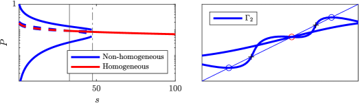
Figure 3.5: Stationary solutions under vanishing feedback. Left: bifurcation diagram as a function of scaling $s$; $\alpha_{N}\mapsto s^{-1}\alpha_{N}$. Below the boundary point defined by (3.25) (dash-dot vertical) there exist two pairs of non-homogeneous solutions, but only one pair is stable. Below the critical value (3.19) (solid vertical) the homogeneous solution is also unstable. Solid/dashed indicates stable/unstable solutions, respectively. Right: illustration of the fix point problem (3.24) when the parameter $s$ is just above and below the limit for existence of non-homogeneous stationary solutions. When $s$ increases, the pair of unstable solutions (plus-signs) approaches the pair of stable solutions (circles) until they collapse into a double root (condition (3.25)), after which only the homogeneous solution remains.

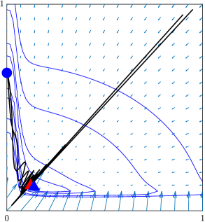
Figure 3.6: Phase-plot of the three-cell problem in the plane which contains all three stationary points. Circle: stable non-homogeneous solution, triangles: unstable solutions with red the homogeneous one. Level curves according to the Euclidean norm of the right-hand side and arrows denote the direction of the flow. Two sample trajectories starting from the upper right corner are also shown, with the oscillations visible before the fate decision.

To sum up, under the proposed parameters from Tab. 2.1 and under weakened feedback $\alpha_{N}\to 0+$, the model undergoes a transition where the typical checkerboard patterning is lost. The two-dimensional generalisation into three cells, as given by (3.21)–(3.22), displays the same stability of post fate decision patterning as consistently observed for the full model when simulated over a grid of multiple connected cells. As an illustration, the overall typical dynamics of the three-cell system is summarised in Fig. 3.6

3.4 System’s Size Convergence

Finally we want to at least qualitatively investigate the RDME model (2.31)–(2.35). As with the ODE model, we first investigate its stability to scaling in the single parameter $\alpha_{N}$. Unlike the ODE model, one is now forced to use a statistical procedure to estimate when the non-homogeneous solutions are lost. This is complicated by the fact that the level of noise is rather large around the transition points, We find in Fig. 3.7 that while the bifurcation behaviour is not as clear as in Fig. 3.5, there is a gradual change of system behaviour approximately around the critical value(s) of scaling $s$, where the system behaviour changes from non-homogeneous (patterned) into homogeneous. In Fig. 3.7 we select the top 25% and bottom 25%, respectively, of the stationary Hes1 protein levels, and plot their means. We use the diameter of each sample as a measure of the spread and judge if the distribution is bimodal or not. Other statistical procedures yield slightly varying results but overall, we find that the RDME behaviour over a mesh is fairly well predicted by the solutions and critical points of the three cell problem.

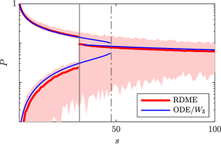
Figure 3.7: Same scaling as in Fig. 3.5, but instead solving the RDME-model on a two-dimensional hex-grid and estimating the mean behaviour of high and low protein concentrations among the cells. The stable solutions of the ODE for the three cell problem from Fig. 3.5 are included for reference.

Finally, we try to measure the quality of the fate decision in the RDME model. For this purpose, recall the coupling matrix $W_{2}(i,j)$ as defined in (3.20), where $i$, $j$ are the two different fates low/high Hes1 protein levels, respectively. For a perfect pattern with two final expression modes (Fig. 3.4 (middle)), the coupling $W_{2}$ is as given in (3.20). To evaluate the behaviour of the RDME model, we seek to estimate the effective coupling matrix from observations. By running multiple independent simulations and splitting the cells of the resulting stationary process into low/high Hes1 expression, we can count how often the specific coupling high-high occurs out of all possible couplings, that is, which corresponds to $W_{2}(2,2)$. We next treat these counts as independent Bernoulli trials and hence the set-up can be practically approached as a statistical estimation problem for a single Bernoulli parameter. The results are summarised in Fig. 3.8 and indicate that even at relatively large levels of noise (corresponding to small cell volume), the patterning is quite close to the perfect one. For example, for mouse embryonal stem cells with a size of about $50\mu m^{3}$, the GRN patterning behaviour is comparably stable to intrinsic cellular noise, with $\hat{p}=0.50(0.43,0.57)$ (95% CI).

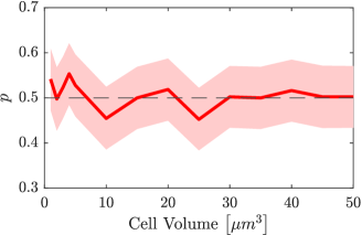
Figure 3.8: A measure of connectivity between high and low protein cells (perfect patterning corresponds to $p=1/2$) for a sequence of volumes in the RDME model (2.31). The numerical problem is treated as a statistical estimation problem for which the confidence intervals are indicated as a shaded area. See text for details.

4 Discussion

Ultimately, we developed a first principle ODE model of the Hes1 pathway and its direct interactions with the Notch pathway, capturing oscillations followed by cell differentiation. We chose parameters based on biological data as much as feasible. By reducing our initial ODE model to lower dimensions, we were able to analyse the differentiation process. Furthermore, we extended the ODE model into a spatial stochastic RDME model to investigate the system’s robustness to intrinsic noise. We found that the transient oscillatory and the differentiation processes observed in the ODE model were well preserved in the RDME model. In this way we have found multiple interlinked ways to model this signalling process, allowing us to investigate multiple aspects of the behaviour of the Hes1-Notch pathway. Linking modeling frameworks in this way forced us to think hard about parameter scaling and parameterisation issues, particularly so in relation to the scarce availability of experimental data.

Our models capture essential aspects of the Hes1-Notch pathway, although they do not replicate every observed behaviour. We observed a few dampened oscillations followed by stable patterning both in the presence and absence of noise. However, the number of oscillations, their stability as well as their length is limited by parameter choice and the interpretation of the states included in the model. As stated in [26], “[t]he molecular mechanism by which cells exhibit different (oscillatory vs. sustained) expression modes of Hes1 is still unknown”. Nevertheless, our results suggest that these distinct expression modes may be intrinsic to the GRN, and thus independent of external regulation.

Despite these promising findings, our models have some limitations. Our model’s oscillations, for example, are longer and more dampened than found in experimental data [18], yet the overall model behaviour is largely stable under noise. While the ODE and RDME behaviour (cf. Fig. 2.3 and Fig. 2.5) show similarities in oscillatory and fate decision behaviours, noise in the stochastic model allows for earlier fate decision in individual cells, thus, leading to less pronounced oscillations in the population average.

Our focus was on the Hes1-Notch pathway isolated from other cellular and signalling processes though we have made simplifications. We did not account for processes such as the dimerisation of the Hes1 protein before it induces mRNA production [25] or other interactions with Notch effectors such as Mash1 [35]. Additionally, the Hes1 pathway interacts with multiple other pathways, such as the cell cycle [30], RBP-J and Jagged [25], as well as the JAK-STAT pathway [26]. These interactions could potentially stabilise the oscillations, which are currently severely dampened in our model. Furthermore, the addition of, for example, extra states or a delay to simulate this behaviour in an ODE system has been shown to allow for more stable oscillations [13, 14, 29, 23, 44]. However, such an extension of our model would further complicate mathematical analysis, which conflicts with our aim of balancing analysability and model complexity.

A major challenge in modelling cellular signalling pathways is the limited availability of data, leading to many models relying heavily or even exclusively on ad hoc parameter values chosen to fit expected model behaviour [16]. As the aim of many Hes1 and Delta-Notch models is to hypothesise about how specific molecular interactions induce cellular and population-level behaviour, the significance of results not based on biologically relevant parameters have to be considered with caution. In our work, this data sparsity has particularly affected the parameters $\alpha_{i},K_{M},K_{n},k$ and $h$. Nevertheless, we have scaled our model behaviour, and thus our parameters, to align with expected biological concentrations for the different constituents to improve the significance of our results. As a point in favour of our approach, the corresponding RDME-model successfully simulates the Hes1-pathway down to the resolution of single species.

There are serveral promising ways to extend the work presented here. Extending the model to incorporate interactions with additional pathways, such as the JAK-STAT pathway or others, could further clarify the dynamics of Hes1 expression. Similarly, adding detail to the Hes1-Notch pathway itself could improve model behaviour and give further insights into its oscillatory and sustained expression modes. Moreover, as the change between these two modes of expression happens during embryonal development to allow for sufficient numbers of neurons and glial cells to develop [26], considering the stability of this signalling process in a growing population becomes exceedingly relevant. Additionally, Hes1 is an important factor in the development of other tissues as well as different cancer types [26] so investigations of the differences between Hes1 interactions in these different tissues could be of interest as well.

To sum up, we have used different modelling approaches to capture the essential behaviours of the Hes1-Notch signalling pathway during neuronal development. By balancing simplicity and analytical tractability, we have constructed models that are both amenable to mathematical analysis and biologically meaningful. Using these models we capture the intrinsic expression of both oscillations and final patterning of this pathway while basing parameters on experimental data as much as possible. While there are improvements or different modelling emphases that can be chosen, our work promotes further understanding of the oscillatory and differentiation processes of this critical signalling pathway.

4.1 Availability and reproducibility

The computational results can be reproduced with release 1.4 of the URDME open-source simulation framework [4], available for download at www.urdme.org. Refer to the Hes1 directory and the associated README.md in the DLCM workflow.

Appendix A Parameterisation

From [19], we know that the average amount of Hes1 protein in a S. cerevisiae cell is $8104$ molecules. Since the yeast cells are roughly similar in size to mouse embryonal stem cells, we assume a size of $50\mu m^{3}$ for both the S. cerevisiae cells and the mouse embryonal stem cells. This gives a wanted Hes1 protein concentration of $0.269\mu M$. For the concentrations of the remaining constituents, we use data from the PaxDB database [21] using the values for the integrated whole organism of the mouse for Dll1, Notch1 and Hes1 while we use the Ngn2 value for the integrated whole organism of humans as this value was not available for mice. Since the values in PaxDB are given in parts per million, we use them to determine the concentrations of the constituents relative to each other. The values used and their scalings relative to Hes1 protein are shown in Tab. A.1. Finally, we use results from [43] to scale the Hes1 mRNA concentration. The authors show that there are $4.2\pm 0.5$ protein molecules per mRNA molecule which gives a Hes1 mRNA concentration of $0.0613\mu M$.

Using this information, we are able to scale $\alpha_{i},K_{M}$ and $K_{n}$ such that the mean stationary behaviour is equal to those wanted concentrations in Tab. A.1. After experimenting with this set-up, we fixed the Hill-functions $K_{M}$ and $K_{n}$ at suitable values such that $\alpha_{i}$ are now uniquely defined as a function of all the other parameters. To find the distributions and confidence intervals of the activation rates, we perturb all degradation rates $\mu_{i}$ assuming they are log-normally distributed with a $68\%$ confidence interval as described in Tab. 2.1. We also perturb the desired concentrations in Tab. A.1, assuming an ad hoc level of $5\%$ relative uncertainty as well as them being log-normally distributed. This way, we find perturbed activation rates $\alpha_{i}$ by fitting model behaviour to our previous requirements. We then fit lognormal distributions to the thus sampled $\alpha_{i}$ to find their confidence intervals as given in Tab. 2.1.

Finally, the distributions for all parameters of the full ODE model in Tab. 2.1 induce distributions of the reduced parameters, which we again find by fitting lognormal distributions to the perturbed reduced parameters, cf. Tab. 2.2.

Molecule	PaxDB Value	Scaled Concentration
Dll1	$0.03$ ppm [M. musculus]	$0.0135\ \mu M$
Notch1	$2.2$ ppm [M. musculus]	$0.925\ \mu M$
Hes1 mRNA	–	$0.0613\ \mu M$
Hes1 protein	$0.639$ ppm [M. musculus]	$0.269\ \mu M$
Ngn2	$0.12$ ppm [H. sapiens]	$0.0505\ \mu M$

Table A.1: Concentration information for the four protein constituents of the model from [21] and scaled to fit relative to Hes1 protein concentration.

Appendix B Dimensional Reduction

To reduce our ODE model (2.7) down to two equations, we rely on quasi-steady state assumptions. To show a typical reduction, we choose the third alternative as shown in Tab. 2.2, i.e. a type 1 reduction. Reductions of type 2 and 3 work equivalently and give the same values for $a$ and $b$. The substitutions in this case are

$$\quad M\leftrightarrow x,\quad D\leftrightarrow y.$$

We assume that the following variables are approximately stationary,

$$\dot{N}\approx 0\implies N =\frac{\alpha_{N}}{\mu_{N}}\langle D_{\text{in}}\rangle,$$

$$\dot{P}\approx 0\implies P =\frac{\alpha_{P}}{\mu_{P}}M,$$

$$\dot{n}\approx 0\implies n =\frac{\alpha_{n}}{\mu_{n}}\frac{1}{1+(P/K_{n})^{k}},$$

where $\langle D_{\text{in}}\rangle\mathrel{\mathop{\ordinarycolon}}=\sum_{i}w_{i}D_{i}$.

This gives

$$\left.\begin{array}[]{rcl}\dot{M}&=&c_{1}\frac{\langle D_{\text{in}}\rangle}{1+c_{2}M^{k}}-\mu_{M}M\\ \dot{D}&=&c_{3}\frac{1}{1+c_{4}M^{h}}-\mu_{D}D\end{array}\right\}$$

with

$$c_{1} =\frac{\alpha_{N}\alpha_{M}}{\mu_{N}},\quad c_{2}=\left(\frac{\alpha_{P}}{\mu_{P}K_{M}}\right)^{k},\quad c_{3}=\frac{\alpha_{D}\alpha_{n}}{\mu_{n}},\quad c_{4}=\left(\frac{\alpha_{P}}{\mu_{P}K_{n}}\right)^{h}.$$

Using the scaling

$$x=\frac{M}{M_{0}},\quad y=\frac{D}{D_{0}},\quad\tilde{t}=\frac{t}{\tau},$$

we find the non-dimensionalised equations

$$\left.\begin{array}[]{rcl}\dot{x}&=&\frac{\langle y_{\text{in}}\rangle}{a+x^{k}}-x\\ \dot{y}&=&v\left(\frac{1}{1+bx^{h}}-y\right)\end{array}\right\}$$

where

$$M_{0}=\left(\frac{c_{1}D_{0}}{\mu_{M}c_{2}}\right)^{\frac{1}{k+1}},\quad D_{0}=\frac{c_{3}}{\mu_{D}},\quad\tau=\frac{1}{\mu_{M}},$$

and

$$a^{-1}=c_{2}M_{0}^{k},\quad b=c_{4}M_{0}^{h},\quad v=\frac{\mu_{D}}{\mu_{M}}.$$

References

- [1] Smita Agrawal, Colin Archer and David V. Schaffer “Computational models of the Notch network elucidate mechanisms of context-dependent signaling” In PLoS Computational Biology 5.5 Public Library of Science, 2009 DOI: https://doi.org/10.1371/journal.pcbi.1000390
- [2] Uri Alon “An Introduction to Systems Biology: Design Principles of Biological Circuits” In Star 10, Mathematical and Computational Biology ChapmanHall/CRC, 2006, pp. 320 URL: http://books.google.com/books?hl=en&lr=&id=tcxCkIxzCO4C&pgis=1
- [3] Spyros Artavanis-Tsakonas, Matthew D. Rand and Robert J. Lake “Notch signaling: Cell fate control and signal integration in development” In Science 284 American Association for the Advancement of Science, 1999, pp. 770–776 DOI: https://doi.org/10.1126/science.284.5415.770
- [4] B., S. and A. “URDME: a modular framework for stochastic simulation of reaction-transport processes in complex geometries” In BMC Syst. Biol. 6.76, 2012, pp. 1–17 DOI: https://doi.org/10.1186/1752-0509-6-76
- [5] Manuel Barrio, Kevin Burrage, André Leier and Tianhai Tian “Oscillatory Regulation of Hes1: Discrete Stochastic Delay Modelling and Simulation” In PLOS Computational Biology 2.9 Public Library of Science, 2006, pp. 1–14 DOI: https://doi.org/10.1371/journal.pcbi.0020117
- [6] Sarah J. Bray “Notch signalling in context” In Nature Reviews Molecular Cell Biology 2016 17:11 17 Nature Publishing Group, 2016, pp. 722–735 DOI: https://doi.org/10.1038/nrm.2016.94
- [7] Herbert Chen et al. “Conservation of the Drosophila lateral inhibition pathway in human lung cancer: a hairy-related protein (HES-1) directly represses achaete-scute homolog-1 expression” In Proceedings of the National Academy of Sciences of the United States of America 94 Proc Natl Acad Sci U S A, 1997, pp. 5355–5360 DOI: https://doi.org/10.1073/PNAS.94.10.5355
- [8] Michael Cohen et al. “Dynamic Filopodia Transmit Intermittent Delta-Notch Signaling to Drive Pattern Refinement during Lateral Inhibition” In Developmental Cell 19 Cell Press, 2010, pp. 78–89 DOI: https://doi.org/10.1016/J.DEVCEL.2010.06.006
- [9] Joanne R Collier, Nicholas A M Monk, Philip K Maini and Julian H Lewis “Pattern Formation by Lateral Inhibition with Feedback: a Mathematical Model of Delta-Notch Intercellular Signalling” In J. theor. Biol 183, 1996, pp. 429–446 DOI: https://doi.org/10.1006/jtbi.1996.0233
- [10] Stefan Engblom “Stochastic Simulation of Pattern Formation in Growing Tissue: A Multilevel Approach” In Bulletin of Mathematical Biology 81 Springer New York LLC, 2019, pp. 3010–3023 DOI: https://doi.org/10.1007/s11538-018-0454-y
- [11] Stefan Engblom, Lars Ferm, Andreas Hellander and Per Lötstedt “Simulation of Stochastic Reaction-Diffusion Processes on Unstructured Meshes” In https://doi.org/10.1137/080721388 31 Society for IndustrialApplied Mathematics, 2009, pp. 1774–1797 DOI: https://doi.org/10.1137/080721388
- [12] Pau Formosa-Jordan, Marta Ibañes, Saúl Ares and José María Frade “Regulation of neuronal differentiation at the neurogenic wavefront” In Development 139 The Company of Biologists, 2012, pp. 2321–2329 DOI: https://doi.org/10.1242/DEV.076406
- [13] Brian C. Goodwin “Oscillatory behavior in enzymatic control processes” In Advances in enzyme regulation 3 Adv Enzyme Regul, 1965 DOI: https://doi.org/10.1016/0065-2571(65)90067-1
- [14] J.. Griffith “Mathematics of cellular control processes. I. Negative feedback to one gene” In Journal of theoretical biology 20 J Theor Biol, 1968, pp. 202–208 DOI: https://doi.org/10.1016/0022-5193(68)90189-6
- [15] Branko Grünbaum and Geoffrey Colin Shephard “Tilings and patterns” W. H. Freeman, 1987
- [16] Jeremy Gunawardena “Models in Systems Biology: The Parameter Problem and the Meanings of Robustness” In Elements of Computational Systems Biology John WileySons, 2010, pp. 21–47 DOI: https://doi.org/10.1002/9780470556757.CH2
- [17] Zena Hadjivasiliou, Ginger L. Hunter and Buzz Baum “A new mechanism for spatial pattern formation via lateral and protrusion-mediated lateral signalling” In Journal of the Royal Society Interface 13 Royal Society of London, 2016 DOI: https://doi.org/10.1098/rsif.2016.0484
- [18] Hiromi Hirata et al. “Oscillatory expression of the BHLH factor Hes1 regulated by a negative feedback loop” In Science 298.5594 American Association for the Advancement of Science, 2002, pp. 840–843 DOI: https://doi.org/10.1126/science.1074560
- [19] Brandon Ho, Anastasia Baryshnikova and Grant W. Brown “Unification of Protein Abundance Datasets Yields a Quantitative Saccharomyces cerevisiae Proteome” In Cell Systems 6 Cell Press, 2018, pp. 192–205.e3 DOI: https://doi.org/10.1016/j.cels.2017.12.004
- [20] Roger A. Horn and Charles R. Johnson “Matrix Analysis” Cambridge, UK: Cambridge Univeristy Press, 1999
- [21] Qingyao Huang et al. “PaxDb 5.0: Curated Protein Quantification Data Suggests Adaptive Proteome Changes in Yeasts” In Molecular and Cellular Proteomics 22 American Society for BiochemistryMolecular Biology Inc., 2023, pp. 100640 DOI: https://doi.org/10.1016/j.mcpro.2023.100640
- [22] Ma Xenia G. Ilagan et al. “Real-time imaging of Notch activation using a Luciferase Complementation-based Reporter” In Science Signaling 4.181 NIH Public Access, 2011, pp. rs7 DOI: https://doi.org/10.1126/SCISIGNAL.2001656
- [23] M.. Jensen, K. Sneppen and G. Tiana “Sustained oscillations and time delays in gene expression of protein Hes1” In FEBS Letters 541 Elsevier, 2003, pp. 176–177 DOI: https://doi.org/10.1016/S0014-5793(03)00279-5
- [24] Caroline Jouve et al. “Notch signalling is required for cyclic expression of the hairy-like gene HES1 in the presomitic mesoderm” In Development 127 The Company of Biologists, 2000, pp. 1421–1429 DOI: 10.1242/DEV.127.7.1421
- [25] Ryoichiro Kageyama, Toshiyuki Ohtsuka and Taeko Kobayashi “The Hes gene family: repressors and oscillators that orchestrate embryogenesis” In Development (Cambridge, England) 134.7 Development, 2007, pp. 1243–1251 DOI: https://doi.org/10.1242/DEV.000786
- [26] Taeko Kobayashi and Ryoichiro Kageyama “Expression dynamics and functions of hes factors in development and diseases” In Current Topics in Developmental Biology 110 Academic Press Inc., 2014, pp. 263–283 DOI: https://doi.org/10.1016/B978-0-12-405943-6.00007-5
- [27] Zi Hao Liu, Xiao Meng Dai and Bin Du “Hes1: A key role in stemness, metastasis and multidrug resistance” In Cancer Biology and Therapy 16.3 Landes Bioscience, 2015, pp. 353–359 DOI: https://doi.org/10.1080/15384047.2015.1016662
- [28] Hiroshi Momiji and Nicholas A.M. Monk “Dissecting the dynamics of the Hes1 genetic oscillator” In Journal of Theoretical Biology 254.4, 2008, pp. 784–798 DOI: https://doi.org/10.1016/j.jtbi.2008.07.013
- [29] Nicholas A.M. Monk “Oscillatory expression of Hes1, p53, and NF-kappaB driven by transcriptional time delays” In Current biology : CB 13.16 Curr Biol, 2003, pp. 1409–1413 DOI: https://doi.org/10.1016/S0960-9822(03)00494-9
- [30] Benjamin Pfeuty “A computational model for the coordination of neural progenitor self-renewal and differentiation through hes1 dynamics” In Development (Cambridge) 142.3 Company of Biologists Ltd, 2015, pp. 477–485 DOI: https://doi.org/10.1242/dev.112649
- [31] Anand Pillarisetti et al. “Mechanical characterization of mouse embryonic stem cells” In Proceedings of the 31st Annual International Conference of the IEEE Engineering in Medicine and Biology Society: Engineering the Future of Biomedicine, EMBC 2009 IEEE Computer Society, 2009, pp. 1176–1179 DOI: https://doi.org/10.1109/IEMBS.2009.5333954
- [32] José Luis De La Pompa et al. “Conservation of the Notch signalling pathway in mammalian neurogenesis” In Development (Cambridge, England) 124 Development, 1997, pp. 1139–1148 DOI: https://doi.org/10.1242/DEV.124.6.1139
- [33] S.. and T.. “Markov Processes: Characterization and Convergence”, Wiley series in Probability and Mathematical Statistics New York: John Wiley & Sons, 1986
- [34] Sana Saleh, Mukhtar Ullah and Hammad Naveed “Role of Cell Morphology in Classical Delta-Notch Pattern Formation” In Proceedings of the Annual International Conference of the IEEE Engineering in Medicine and Biology Society, EMBS 2021-January Institute of ElectricalElectronics Engineers Inc., 2021, pp. 4139–4142 DOI: https://doi.org/10.1109/EMBC46164.2021.9630053
- [35] Hiromi Shimojo, Toshiyuki Ohtsuka and Ryoichiro Kageyama “Dynamic expression of Notch signaling genes in neural stem/ progenitor cells” In Frontiers in Neuroscience, 2011 DOI: https://doi.org/10.3389/fnins.2011.00078
- [36] Hiromi Shimojo et al. “Oscillatory control of Delta-like1 in cell interactions regulates dynamic gene expression and tissue morphogenesis” In Genes & development 30 Genes Dev, 2016, pp. 102–116 DOI: 10.1101/GAD.270785.115
- [37] D Sprinzak et al. “Mutual Inactivation of Notch Receptors and Ligands Facilitates Developmental Patterning” In PLoS Comput Biol 7, 2011, pp. 1002069 DOI: https://doi.org/10.1371/journal.pcbi.1002069
- [38] Marc Sturrock, Andreas Hellander, Anastasios Matzavinos and Mark A.J. Chaplain “Spatial stochastic modelling of the Hes1 gene regulatory network: intrinsic noise can explain heterogeneity in embryonic stem cell differentiation” In Journal of The Royal Society Interface 10 The Royal Society, 2013 DOI: https://doi.org/10.1098/RSIF.2012.0988
- [39] Marc Sturrock et al. “The Role of Dimerisation and Nuclear Transport in the Hes1 Gene Regulatory Network” In Bulletin of Mathematical Biology 76 Springer ScienceBusiness Media, LLC, 2014, pp. 766–798 DOI: https://doi.org/10.1007/s11538-013-9842-5
- [40] Hendrik B. Tiedemann et al. “Modeling coexistence of oscillation and Delta/Notch-mediated lateral inhibition in pancreas development and neurogenesis” In Journal of Theoretical Biology 430 Academic Press, 2017, pp. 32–44 DOI: https://doi.org/10.1016/j.jtbi.2017.06.006
- [41] Jonathan M.D. Vosper et al. “Regulation of neurogenin stability by ubiquitin-mediated proteolysis” In Biochemical Journal 407.2, 2007, pp. 277–284 DOI: https://doi.org/10.1042/BJ20070064
- [42] J. Wang, P. Alexander and S.. McKnight “Metabolic specialization of mouse embryonic stem cells” In Cold Spring Harbor Symposia on Quantitative Biology 76, 2011, pp. 183–193 DOI: https://doi.org/10.1101/sqb.2011.76.010835
- [43] Ji Yu et al. “Probing gene expression in live cells, one protein molecule at a time” In Science 311, 2006, pp. 1600–1603 DOI: https://doi.org/10.1126/SCIENCE.1119623
- [44] Stefan Zeiser, Johannes Müller and Volkmar Liebscher “Modeling the Hes1 oscillator” In Journal of Computational Biology 14, 2007, pp. 984–1000 DOI: https://doi.org/10.1089/cmb.2007.0029