Space-Air-Ground Integrated MEC-Assisted Industrial Cyber-Physical Systems: An Online Decentralized Optimization Approach

Abstract

Cloud computing and edge/fog computing are playing a pivotal role in driving the transformation of industrial cyber-physical systems (ICPS) towards greater intelligence and automation by providing high-quality computation offloading services to Internet of Things devices (IoTDs). Recently, space-air-ground integrated multi-access edge computing (SAGIMEC) is emerging as a promising architecture combining edge computing and cloud computing, which has the potential to be integrated with ICPS to accelerate the realization of the above vision. In this work, we first present an SAGIMEC-assisted ICPS architecture that incorporates edge computing and cloud computing through seamless connectivity supported by satellite networks to achieve determinism in connectivity, networked computing, and intelligent networked control. Then, we formulate a joint satellite selection, computation offloading, communication resource allocation, computation resource allocation, and UAV trajectory control optimization problem ($\text{JSC}^{4}\text{OP}$) to maximize the quality of service (QoS) of IoTDs. This problem considers both the dynamics and uncertainties of the system environment, as well as the limited resources and energy of UAVs. Given the complexity of $\text{JSC}^{4}\text{OP}$, we propose an online decentralized optimization approach (ODOA) to solve the problem. Specifically, $\text{JSC}^{4}\text{OP}$ is first transformed into a real-time decision-making optimization problem (RDOP) by leveraging Lyapunov optimization. Then, to solve the RDOP, we introduce an online learning-based latency prediction method to predict the uncertain system environment and a game theoretic decision-making method to make real-time decisions. Finally, theoretical analysis confirms the effectiveness of the ODOA, while the simulation results demonstrate that the proposed ODOA outperforms other alternative approaches in terms of overall system performance.

I Introduction

With the rapid advancement of communication technologies and Internet of Things (IoT), industrial cyber-physical systems (ICPS) are increasingly becoming a crucial pillar in driving the transition of industry 4.0 towards intelligence and automation [1]. Specifically, the vision of ICPS is to integrate the physical processes of IoT devices (IoTDs) with the computational and communication capabilities of networks, thereby stimulating a wide range of intelligent applications that significantly enhance industrial production efficiency. However, a key challenge lies in the fact that enabling these intelligent applications typically requires handling a large volume of latency-sensitive and computation-heavy tasks, which conflicts with the limited computational resources and energy consumption of IoTDs.

The integration of cloud computing and edge computing into ICPS has garnered significant attention as a viable solution, providing computing offloading services with high quality of service (QoS) for IoTDs. For example, Cao et al. [2] provided a comprehensive review of edge and edge-cloud computing-assisted ICPS architectures, in which the cloud computing and edge computing are combined into ICPS by deploying ground infrastructure. Li et al. [3] considered an industrial cyber-physical IoT system that utilizes the cloud data centers to achieve centralized control and processing. Hao et al. [4] proposed a softwarized-based ICPS architecture, where multiple terrestrial edge clouds are deployed to provide data analysis and processing for the ICPS. However, the aforementioned research on cloud or edge computing-assisted ICPS architectures heavily relies on the deployment of ground infrastructure, which may lead to the high deployment costs, limited coverage, and constrained application scenarios. For instance, in remote or disaster-stricken areas where the ground infrastructure is either nonexistent or unavailable, these architectures may struggle to operate effectively.

To overcome the abovementioned challenges, space-air-ground integrated multi-access edge computing (SAGIMEC) is emerging as a promising architecture to provide edge and cloud computing services. Specifically, SAGIMEC is usually a three-tier computing architecture that integrates heterogeneous network components, including a terrestrial base station network, an aerial UAV network, and a space low earth orbit (LEO) satellite network [5]. First, thanks to the wide coverage of LEO satellites and flexible mobility of UAVs, SAGIMEC greatly expands the application scenarios and coverage of edge computing. Furthermore, the low transmission latency and seamless connectivity of LEO satellites enable SAGIMEC to effectively combine cloud-edge computing resources to improve the resource utilization. Therefore, SAGIMEC showcases substantial promise in propelling the evolution of ICPS.

Several studies have investigated the SAGIMEC network. For example, to minimize the total system latency of the SAGIMEC network, Cheng et al. [6] jointly optimized the resource allocation and computation offloading. Fan et al. [7] formulated an optimization problem of joint resource allocation and computation offloading to reduce the system cost, which consists of the system energy consumption and system latency. To achieve higher system energy efficiency, Hu et al. [8] formulated the optimization problem of UAV trajectory control and resource allocation. However, the aforementioned studies above usually assume that the satellite link status can be accurately measured, which may be impractical because of the high-speed mobility, long-distance transmission, and time-varying network topology of satellite networks. Moreover, these studies usually formulate the optimization problems from the system perspective to consider indicators such as energy consumption and latency, which may neglect the QoS for IoTDs.

Fully exploring the benefits of combining SAGIMEC with ICPS faces several fundamental challenges. i) Computation Offloading. The heterogeneity of the networks in SAGIMEC leads to an uneven distribution of resources. Moreover, different IoTDs usually have diverse computing requirements for resources. As a result, the heterogeneous resource distribution and IoTD requirements lead to the complexity of computation offloading decisions. ii) Satellite Selection. The dynamic topology of satellite networks leads to time-varying and uncertain satellite link conditions. Therefore, when multiple satellites are accessible, it is challenging to select appropriate satellites as relay nodes for the efficient use of cloud computing services based on satellite networks. iii) Resource Management. The tasks of IoTDs are often computation-heavy and latency-sensitive, imposing strict requirements on computing and communication resources. However, UAV networks usually have limited computing and spectrum resources. Therefore, the strict computing requirements make resource allocation difficult in the resource-constrained UAV network. iv) Trajectory Control. While the mobility of UAVs enhances the elasticity and flexibility of MEC, it also introduces important challenges related to UAV trajectory control. Furthermore, the limited battery capacity of UAVs leads to finite service time, which requires balancing both the service time of UAVs and the QoS of IoTDs.

The abovementioned challenges necessitate efficient optimization of computation offloading, satellite selection, resource allocation, and UAV trajectory control. However, focusing on just one aspect of these components is insufficient to fully explore the advantages of SAGIMEC-assisted ICPS. First, these optimization variables are mutually coupled. For example, optimizing computation offloading requires the simultaneous consideration of satellite selection, resource allocation, and UAV location. Second, these optimization variables collectively determine the QoS of IoTDs. Therefore, these coupled optimization variables should be jointly optimized to fully exploit the performance of SAGIMEC-assisted ICPS, as it can effectively capture the intricate and coupling interactions and trade-offs among various optimization components. Consequently, we propose a novel online decentralized optimization approach (ODOA) that enables the joint optimization of computation offloading, satellite selection, communication resource allocation, computation resource allocation, and UAV trajectory control, to effectively improve the performance of SAGIMEC-assisted ICPS. Furthermore, compared to other approaches such as deep reinforcement learning (DRL), the proposed ODOA is more suitable for the considered system by leveraging the strengths of Lyapunov optimization, online learning, and game theory. Specifically, Lyapunov optimization is good for real-time decision-making without requiring direct knowledge of system dynamics and provides interpretability. Moreover, game theory can decentralized decision-making and guarantee existence of a solution, making the ODOA more scalable. Our main contributions are outlined as follows:

• System Architecture. We propose an SAGIMEC-assisted ICPS architecture, where a UAV and a cloud computing center are seamlessly connected via a satellite network to facilitate high-quality computing offload services. Moreover, within this architecture, we consider the time-varying computing requirements of IoTDs, the energy and resource constraints of the UAV, as well as the dynamics and uncertainties of the satellite links to more accurately capture the real-world physical characteristics of SAGIMEC-assisted ICPS.

• Problem Formulation. We formulate a joint satellite selection, computation offloading, communication and computation resource allocation, and UAV trajectory control optimization problem ($\text{JSC}^{4}\text{OP}$) to maximize the QoS of IoTDs. Moreover, we show that the formulated $\text{JSC}^{4}\text{OP}$ is difficult to solve directly because it depends on future information and contains uncertain network parameters. In addition, we demonstrate that the $\text{JSC}^{4}\text{OP}$ is non-convex and NP-hard.

• Approach Design. Since the $\text{JSC}^{4}\text{OP}$ is difficult to be directly solved, we propose the ODOA. Specifically, we first transform the $\text{JSC}^{4}\text{OP}$ into a real-time decision-making optimization problem (RDOP) that only depends on current information by using the Lyapunov optimization. Then, for the RDOP, we propose an online learning-based latency prediction method to predict uncertain network parameters and a game theoretic decision-making method to make real-time decisions.

• Performance Evaluation. The effectiveness and performance of the designed ODOA are confirmed through theoretical analysis and simulation experiments. In particular, the theoretical analysis proves that the ODOA not only satisfies the UAV energy consumption constraint, but also exhibits polynomial complexity. Additionally, the simulation results demonstrate that the ODOA outperforms other alternative approaches in terms of the overall system performance.

The subsequent sections of this work are structured as follows. We introduce the relevant models and problem formulation in Section II. We detail the proposed ODOA and theoretical analysis in Section III. In Section IV, we demonstrate and discuss simulation results. Lastly, we present the conclusions in Section V.

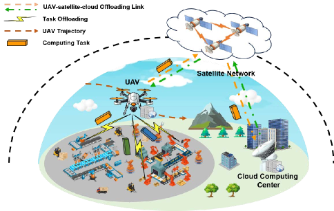
Figure 1: The proposed SAGIMEC-assisted ICPS architecture.

II System Model and Problem Formulation

As depicted in Fig. 1, we consider an SAGIMEC-assisted ICPS to deliver reliable computing offloading services for IoTDs. Specifically, in the spatial dimension, the proposed system is structured as a hierarchical architecture consisting of a terrestrial layer, an aerial layer, and a space layer, which are described in detail below.

At the terrestrial layer, a set of IoTDs $\mathcal{M}=\{1,\ldots,M\}$ are distributed in the considered area to perform specific industrial activities such as monitoring or data collection, and generate computing tasks with time-varying computational demands. Moreover, a cloud computing center $c$ is located far from the service area, which can provide robust cloud computing services. However, due to the lack of ground communication facilities, such as in deserts or plateau areas, the IoTDs are unable to access the cloud computing center via the terrestrial network. At the aerial layer, a rotary-wing UAV $u$ equipped with computational capabilities is employed in close proximity to the IoTDs to provide flexible computing offloading services. Furthermore, the UAV acts as a software-defined networking (SDN) controller, responsible for gathering network information and making relevant decisions. At the space layer, we consider a satellite network consisting of $N$ LEO satellites. This satellite network provides seamless communication connectivity between the UAV and the cloud computing center, thereby making cloud computing services accessible.

In the temporal dimension, the system operates in a discrete time slot manner. Specifically, the system time is partitioned into $T$ equal time slots, denoted by $t\in\mathcal{T}=\{1,\ldots,T\}$, each with a duration of $\tau$ [9]. Furthermore, $\tau$ is selected to be sufficiently small to ensure that each time slot can be considered as quasi-static [10].

II-A Basic Model

IoTD Model. We consider that each IoTD generates a computing task per time slot [11, 12]. At time slot $t$, the attributes of IoTD $m\in\mathcal{M}$ can be characterized as $\mathbf{St}_{m}(t)=\left(f_{m}^{\text{IoTD}},\mathbf{\Phi}_{m}(t),\mathbf{q}_{m}\right)$, where $f_{m}^{\text{IoTD}}$ denotes the local computing capability of IoTD $m$. Furthermore, the set $\mathbf{\Phi}_{m}(t)=\{D_{m}(t),\eta_{m}(t),T^{\text{max}}_{m}(t)\}$ represents the attributes of the computing task generated by IoTD $m$, where $D_{m}(t)$ indicates the task data size (in bits), $\eta_{m}(t)$ denotes the computation density (in cycles/bit), and $T^{\text{max}}_{m}(t)$ is the deadline of the task (in seconds). Moreover, $\mathbf{q}_{m}=\left[x_{m},y_{m}\right]$ stands for the location coordinates of IoTD $m$.

UAV Model. Similar to [13], we consider that the UAV flies at a fixed altitude $H$ to mitigate additional energy consumption associated with frequent altitude changes. Therefore, the UAV $u$ can be characterized by $\mathbf{St}_{u}(t)=(\mathbf{q}_{u}^{t},H,F_{u}^{\text{max}})$, where $\mathbf{q}_{u}^{t}=[x_{u}^{t},y_{u}^{t}]$ and $H$ represent the horizontal coordinates and flight height, respectively. Moreover, $F_{u}^{\text{max}}$ denotes the total computing resources.

Satellite Model. Due to the movement of satellites, the connectivity between the UAV and satellites varies over time, leading to a time-varying subset of accessible satellites $\mathcal{S}(t)$. Furthermore, due to the periodic nature of satellite movements, the concept of snapshots can be utilized to model the changes of the accessible subset [14]. Specifically, every $\Delta$ consecutive time slots form a snapshot epoch, where the accessible subset remains constant within each snapshot epoch but varies across different snapshot epochs [15].

II-B Task Computing Model

The task $\mathbf{\Phi}_{m}(t)$ generated by IoTD $m$ can be carried out locally on the IoTD (referred to as local computing), offloaded to UAV $u$ for execution (referred to as UAV-assisted computing), or offloaded to cloud $c$ for execution (referred to as cloud-assisted computing), which is decided by the offloading decision of the IoTD. Therefore, at time slot $t$, we define a variable $a_{m}(t)\in\{l,u,c\}$ to indicate the offloading decision of IoTD $m$, where $a_{m}(t)=l$ indicates the local computing, $a_{m}(t)=u$ represents the UAV-assisted computing, and $a_{m}(t)=c$ signifies the cloud-assisted computing. Furthermore, both local computing and computation offloading generally involve overheads in terms of latency and energy, which are explained in detail below.

II-B1 Local Computing

If task $\mathbf{\Phi}_{m}(t)$ is processed locally by IoTD $m$ at time slot $t$, the IoTD utilizes its local computational resources to execute the task.

Task Completion Latency. The task completion latency for local computing is computed as $T_{m}^{\text{LC}}(t)=\eta_{m}(t)D_{m}(t)/f_{m}^{\text{IoTD}}$, where $f_{m}^{\text{IoTD}}$ represents the computing capability of IoTD $m$.

IoTD Computation Energy Consumption. The energy consumption of IoTD $m$ to execute task $\mathbf{\Phi}_{m}(t)$ is given as $E_{m}^{\text{LC}}(t)=k(f_{m}^{\text{IoTD}})^{3}T_{m}^{\text{LC}}(t)$, where $k$ is the effective switched capacitance coefficient [16].

II-B2 UAV-assisted Computing

If task $\mathbf{\Phi}_{m}(t)$ is offloaded to UAV $u$ for execution at time slot $t$, the UAV establishes a communication connection with IoTD $m$ to receive the task, allocates computing resources for task execution, and transmits the processed results to the IoTD. Note that the latency and energy consumption associated with the result feedback are disregarded, owing to the short-distance transmission and the small data size of the feedback [14].

IoTD-UAV Communication. The widely used orthogonal frequency-division multiple access (OFDMA) is applied by the UAV to simultaneously serve multiple IoTDs [17]. According to Shannon’s formula, at time slot $t$, the data transmission rate from IoTD $m$ to UAV $u$ is expressed as $R_{u,m}(t)=w_{u,m}^{t}B_{u}\log_{2}\big{(}1+P_{m}g_{u,m}(t)/\varpi_{0}\big{)}$, where $w_{u,m}^{t}\in(0,1]$ represents the resource allocation coefficient of IoTD $m$, $B_{u}$ denotes the bandwidth resources available to UAV $u$, $P_{m}$ indicates the transmission power of IoTD $m$, $\varpi_{0}$ is the noise power, and $g_{u,m}(t)$ means the channel gain.

Considering that the IoTD-UAV link may experience obstruction from environmental obstacles, we employ the widely used probabilistic line-of-sight (LoS) channel model to describe the communication condition [18]. Specifically, the LoS probability $\rho_{u,m}^{\text{LoS}}(t)$ from UAV $u$ to IoTD $m$ is defined as $\rho_{u,m}^{\text{LoS}}(t)=1/(1+c_{1}\exp(-c_{2}((180/\pi)\arcsin{(H/d_{u,m}(t))}-c_{1})))$, where $c_{1}$ and $c_{2}$ are the constants depending on the environment, and $d_{u,m}(t)$ means the straight-line distance between UAV $u$ and IoTD $m$ [19]. Similar to [20], the path loss between IoTD $m$ and UAV $u$ is assessed as

$$L_{u,m}(t)= 20\log_{10}\big{(}4\pi f_{u}d_{u,m}(t)/v_{c}\big{)}+\rho_{u,m}^{\text{LoS}}(t)\eta^{\text{LoS}}$$ (1)

$$+\big{(}1-\rho_{u,m}^{\text{LoS}}(t)\big{)}\eta^{\text{nLoS}},$$

where $f_{u}$ represents the carrier frequency, and $v_{c}$ indicates the speed of light. $\eta^{\text{nLoS}}$ and $\eta^{\text{LoS}}$ denote the extra losses for nLoS and LoS links, respectively. Generally, the channel gain $g_{u,m}(t)$ is estimated as $g_{u,m}(t)=10^{-L_{u,m}/10}$.

Task Completion Latency. The task completion latency primarily comprises both transmission and execution delay, which is calculated as

$$\small T_{m}^{\text{UC}}(t)=D_{m}(t)/R_{u,m}(t)+\eta_{m}(t)D_{m}(t)/F_{u,m}^{t},$$ (2)

where $F_{u,m}^{t}$ stands for the computational resources assigned by UAV $u$ to IoTD $m$ at time slot $t$.

IoTD Transmission Energy Consumption. For UAV-assisted computing, the transmission energy consumption of IoTD is computed as

$$\small E_{m}^{\text{UC}}(t)=P_{m}D_{m}(t)/R_{u,m}(t).$$ (3)

UAV Computation Energy Consumption. The computation energy consumption of UAV for UAV-assisted computing is given as

$$\small E_{u,m}^{\text{comp}}(t)=\varpi\eta_{m}(t)D_{m}(t),$$ (4)

where $\varpi$ denotes the energy consumed for each unit of CPU cycle by the UAV [12].

Therefore, at time slot $t$, the total computational energy consumption of the UAV is given as

$$\small E_{u}^{\text{comp}}(t)=\sum_{m\in\mathcal{M}}I_{\{a_{m}(t)=u\}}E_{u,m}^{\text{comp}}(t),$$ (5)

where $I_{\{X\}}$ represents an indicator function that equals 1 if $X$ holds true, and 0 otherwise.

II-B3 Cloud-assisted Computing

If task $\mathbf{\Phi}_{m}(t)$ is offloaded to cloud $c$ for execution at time slot $t$, it is initially offloaded to the UAV. Then, the UAV further offloads the task to the cloud via the satellite network relay and receives the result feedback from the cloud. However, unlike IoTD-UAV communication, the UAV-satellite-cloud channel is severely affected by long-distance transmission, unpredictable weather conditions, high-speed satellite mobility, and dynamic satellite network topology [21]. Therefore, measuring the round-trip latency of tasks for UAV-satellite-cloud transmission accurately is challenging. Moreover, there are multiple accessible satellites, as indicated in the set $\mathcal{S}(t)$, per time slot. The selection of different satellite relays may result in varying round-trip latency. To this end, we introduce variables $b_{u}^{t}\in\mathcal{S}(t)$ and $L_{s}(t)$ to represent the satellite selection decision and the unit data round-trip latency for satellite $s\in\mathcal{S}(t)$, respectively. Specifically, the variable $L_{s}(t)$ ($L_{s}^{\text{min}}\leq L_{s}(t)\leq L_{s}^{\text{max}}$) stands for a random variable with an unknown mean, which is assumed to be independently and identically distributed across time slots [22].

Task Completion Latency. The task completion latency primarily composed of the transmission delay from IoTD $m$ to the UAV, the round-trip delay from the UAV to the cloud, and the cloud computing delay. Considering that cloud computing has sufficient computational resources, we ignore the corresponding computing delay. Therefore, the task completion latency is given as

$$\small T_{m}^{\text{CC}}(t)=D_{m}/R_{u,m}(t)+\sum_{s\in\mathcal{S}(t)}I_{\{b_{u}^{t}=s\}}D_{m}(t)L_{s}(t).$$ (6)

IoTD Transmission Energy Consumption. For cloud-assisted computing, the IoTD incurs transmission energy consumption, i.e.,

$$\small E_{m}^{\text{CC}}(t)=P_{m}D_{m}(t)/R_{u,m}(t).$$ (7)

UAV Transmission Energy Consumption. Similarly, the UAV also incurs transmission energy consumption for cloud-assisted computing, which is calculated as

$$\small E_{u,m}^{\text{trans}}=\sum_{s\in\mathcal{S}(t)}I_{\{b_{u}^{t}=s\}}D_{m}(t)Z_{s}(t),$$ (8)

where $Z_{s}(t)$ denotes the energy required to transmit each bit of data between the UAV and satellite $s$ at time slot $t$. Therefore, the total transmission energy consumption of the UAV is obtained as

$$\small E_{u}^{\text{trans}}(t)=\sum_{m\in\mathcal{M}}I_{\{a_{m}^{t}=c\}}E_{u,m}^{\text{trans}}(t).$$ (9)

II-C Total UAV Energy Consumption

At time slot $t$, the total energy consumption of the UAV includes propulsion energy consumption, transmission energy consumption, and computation energy consumption. Similar to [23, 24], the propulsion power for a rotary-wing UAV with speed $v_{u}$ is given as

$$\small P_{u}(v_{u})=\underbrace{C_{1}(1+3v_{u}^{2}/U_{\text{p}}^{2})}_{\text{blade profile }}+\underbrace{C_{2}\sqrt{\sqrt{C_{3}+v_{u}^{4}/4}-v_{u}^{2}/2}}_{\text{induced }}+\underbrace{C_{4}v_{u}^{3}}_{\text{parasite}},$$ (10)

where $U_{\text{p}}$ refers to the rotor’s tip speed, $C1$, $C2$, $C3$, and $C4$ are the constants defined in [25]. Therefore, at time slot $t$, the total energy consumption of the UAV is calculated as

$$\small E_{u}(t)=E_{u}^{\text{comp}}(t)+E_{u}^{\text{trans}}(t)+E_{u}^{\text{prop}}(t),$$ (11)

where $E_{u}^{\text{prop}}(t)=P_{u}(v_{u}(t))\tau$ denotes the propulsion energy consumption. To guarantee service time, the UAV energy consumption constraint is defined as

$$\small\lim_{T\rightarrow+\infty}\frac{1}{T}\sum_{t=1}^{T}\mathbb{E}\left\{E_{u}(t)\right\}\leq\bar{E}_{u},$$ (12)

where $\bar{E}_{u}$ is the energy budget of the UAV per time slot.

II-D Performance Metrics

We evaluate the QoS of each IoTD in each time slot by jointly considering the task completion latency cost and the IoTD energy consumption cost. Specifically, at time slot $t$, the task completion latency of IoTD $m$ is given as

$$\small T_{m}(t)=I_{\{a_{m}^{t}=l\}}T_{m}^{\text{LC}}+I_{\{a_{m}^{t}=u\}}T_{m}^{\text{UC}}+I_{\{a_{m}^{t}=c\}}T_{m}^{\text{CC}}.$$ (13)

Accordingly, at time slot $t$, the energy consumption of IoTD $m$ is described as

$$\small E_{m}(t)=I_{\{a_{m}^{t}=l\}}E_{m}^{\text{LC}}+I_{\{a_{m}^{t}=u\}}E_{m}^{\text{UC}}+I_{\{a_{m}^{t}=c\}}E_{m}^{\text{CC}}.$$ (14)

Similar to [26, 27], at time slot $t$, the cost of IoTD $m$ is formulated as

$$\small C_{m}(t)=\gamma^{\text{T}}T_{m}(t)+\gamma^{\text{E}}E_{m}(t),$$ (15)

where $\gamma^{\text{T}}$ and $\gamma^{\text{E}}$ (with $\gamma^{\text{T}}+\gamma^{\text{E}}=1$) respectively denote the weighting coefficients of latency and energy consumption. Clearly, minimizing the cost of IoTDs is equivalent to maximizing the QoS of IoTDs.

II-E Problem Formulation

To maximize the QoS of all IoTDs over time (i.e., minimize the time-averaged costs of all IoTDs), this work jointly optimizes the computation offloading $\mathbf{A}=\{\mathcal{A}^{t}|\mathcal{A}^{t}=\{a_{m}^{t}\}_{m\in\mathcal{M}}\}_{t\in\mathcal{T}}$, satellite selection $\mathbf{B}=\{b_{u}^{t}\}_{t\in\mathcal{T}}$, computing resource allocation $\mathbf{F}=\{\mathcal{F}^{t}|\mathcal{F}^{t}=\{F_{u,m}^{t}\}_{m\in\mathcal{M}}\}_{t\in\mathcal{T}}$, communication resource allocation $\mathbf{W}=\{\mathcal{W}^{t}|\mathcal{W}^{t}=\{w_{u,m}^{t}\}_{m\in\mathcal{M}}\}_{t\in\mathcal{T}}$, and UAV trajectory control $\mathbf{Q}=\{\mathbf{q}_{u}^{t}\}_{t\in\mathcal{T}}$. This optimization problem can be mathematically formulated as follows:

$$\textbf{P}:\quad \underset{\mathbf{A},\mathbf{B},\mathbf{F},\mathbf{W},\mathbf{Q}}{\text{min}}\frac{1}{T}\sum_{t=1}^{T}\sum_{m=1}^{M}C_{m}(t)$$ (16)

s.t. $$\lim_{T\rightarrow+\infty}\frac{1}{T}\sum_{t=1}^{T}\mathbb{E}\left\{E_{u}(t)\right\}\leq\bar{E}_{u},$$ (16a)

$$a_{m}^{t}\in\{l,u,c\},\forall m\in\mathcal{M},t\in\mathcal{T},$$ (16b)

$$I_{\{a_{m}^{t}=u\}}T^{\text{UC}}_{m}(t)+I_{\{a_{m}^{t}=c\}}T^{\text{CC}}_{m}(t)\leq T_{m}^{\text{max}},\forall m\in\mathcal{M},t\in\mathcal{T},$$ (16c)

$$b_{u}^{t}\in\mathcal{S}(t),\forall t\in\mathcal{T},$$ (16d)

$$0<F_{u,m}^{t}\leq F_{u}^{\text{max}},\forall m\in\mathcal{M},t\in\mathcal{T},$$ (16e)

$$\sum_{m\in\mathcal{M}}I_{\{a_{m}^{t}=u\}}F_{u,m}^{t}\leq F_{u}^{\text{max}},\forall t\in\mathcal{T},$$ (16f)

$$0<w_{u,m}^{t}\leq 1,\forall m\in\mathcal{M},\forall t\in\mathcal{T},$$ (16g)

$$\sum_{m\in\mathcal{M}}I_{\{a_{m}^{t}\in\{u,c\}\}}w_{u,m}^{t}\leq 1,\forall t\in\mathcal{T},$$ (16h)

$$\mathbf{q}_{u}^{t=1}=\mathbf{q}^{\text{ini}},$$ (16i)

$$||\mathbf{q}_{u}^{t+1}-\mathbf{q}_{u}^{t}||\leq v_{u}^{\text{max}}\tau,\forall t\in\mathcal{T},$$ (16j)

where $\mathbf{q}^{\text{ini}}$ represents the initial position of the UAV. Constraint (16a) is the long-term UAV energy consumption constraint. Constraints (16b) and (16c) pertain to computation offloading decisions. Constraint (16d) states that the UAV can only choose one satellite for communication. Constraints (16e) and (16f) regulate the allocation of computing resources, while constraints (16g) and (16h) constrain the allocation of communication resources. Finally, constraints (16i) and (16j) concern the UAV trajectory control.

Problem Analysis: There are three main challenges in optimally solving the problem P. i) Future-dependent. Obtaining the optimal solution of the problem requires complete future information, e.g., computing demands of all IoTDs across all time slots. However, acquiring the future information is very challenging in the considered time-varying scenario. ii) Uncertainty. Since the problem involves an uncertain network parameter, i.e., the task round-trip latency between the UAV and the cloud, it is challenging to make relevant decisions under uncertain network dynamics. iii) Non-convex and NP-hard. The problem involves both continuous variables (i.e., resource allocation $\{\mathbf{F},\mathbf{W}\}$ and UAV trajectory control $\mathbf{Q}$) and discrete variables (i.e., computation offloading decision $\mathbf{A}$ and satellite selection decision $\mathbf{B}$). Therefore, it is a mixed-integer non-linear programming (MINLP) problem, which can be proven to be non-convex and NP-hard [28, 29].

III Online Decentralized Optimization Approach

In the section, we first present the motivation for proposing ODOA. Then, we elaborate on the framework of the proposed ODOA.

III-A Motivation of Proposing ODOA

For the complex problem P, although DRL is often considered a viable approach, it may not be suitable for the considered system for the following reasons. First, DRL typically requires a substantial number of training samples to learn effective strategies. However, due to the time-varying and uncertain nature of the system, obtaining real sample data is challenging. Moreover, the formulated optimization problem involves numerous constraints, a high-dimensional decision space, and heterogeneous attributes of the decision variables. Therefore, using DRL to solve this problem faces convergence challenges. Furthermore, DRL is highly sensitive to environmental changes and lacks interpretability, which poses challenges in fulfilling the requirements of the system for scalability and adaptability.

Accordingly, we proposed an efficient approach, i.e., ODOA, by leveraging Lyapunov optimization, online learning and game theory to transform and decompose the original problem based on the specific characteristics of the considered system and the optimization problem. Compared to DRL, the proposed approach does not require sample data and explicit knowledge of the system dynamics. Additionally, the proposed approach offers interpretability and broader adaptability. Finally, the proposed approach has low computational complexity, rendering it appropriate for real-time decision-making. Fig. 2 despicted the framework of ODOA, and the details are elaborated in the following.

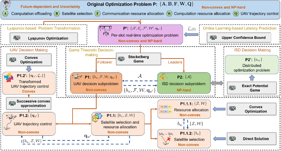
Figure 2: The framework of ODOA.

III-B Lyapunov-Based Problem Transformation

Since problem P is future-dependent, an online approach is necessary for real-time decision making without foreseeing the future. The Lyapunov optimization framework is a commonly used approach for online approach design, as it does not require direct knowledge of the network dynamics while providing guaranteed performance [25]. Consequently, we first reformulate problem P into a per-slot real-time optimization problem by using Lyapunov optimization.

Specifically, to address the UAV energy constraint (16a), we define two virtual energy queues $Q_{u1}(t)$ and $Q_{u2}(t)$ to represent the total transmission and computing energy queue, as well as the propulsion energy queue at time slot $t$, respectively. Moreover, these queues are set as zero at the initial time slot, i.e., $Q_{u1}(1)=0$ and $Q_{u2}(1)=0$. Specifically, the virtual energy queues evolves as follows:

$$\small\begin{cases}Q_{u1}(t+1)=\max\left\{Q_{u1}(t)+E_{u1}(t)-\bar{E_{u1}},0\right\},\\ Q_{u2}(t+1)=\max\left\{Q_{u2}(t)+E_{u2}(t)-\bar{E_{u2}},0\right\},\end{cases}$$ (17)

where $E_{u1}(t)=E_{u}^{\text{comp}}(t)+E_{u}^{\text{trans}}(t)$ and $E_{u2}(t)=E_{u}^{\text{prop}}(t)$. Furthermore, $\bar{E_{u1}}$ and $\bar{E_{u2}}$ (with $\bar{E_{u1}}+\bar{E_{u2}}=\bar{E_{u}}$) represent the computing and transmission energy budgets per slot, as well as the propulsion energy budgets per slot, respectively.

Second, to achieve a scalar measure of the queue backlogs, we define the Lyapunov function $L(\boldsymbol{\Theta}(t))$ as follows:

$$\small L(\boldsymbol{\Theta}(t))=((Q_{u1}(t))^{2}+(Q_{u2}(t))^{2})/{2},$$ (18)

where $\boldsymbol{\Theta}(t)=[Q_{u1}(t),Q_{u2}(t)]$ denotes the current queue backlogs. Third, the conditional Lyapunov drift for time slot $t$ can be defined as

$$\small\Delta L(\boldsymbol{\Theta}(t))\triangleq\mathbb{E}\{L(\boldsymbol{\Theta}(t+1))-L(\boldsymbol{\Theta}(t))\mid\boldsymbol{\Theta}(t)\}.$$ (19)

Finally, similar to [30, 12, 25], the drift-plus-penalty is given as

$$\small D(\boldsymbol{\Theta}(t))=\Delta L(\boldsymbol{\Theta}(t))+V\mathbb{E}\left\{C_{s}(t)\mid\mathbf{\Theta}(t)\right\},$$ (20)

where $C_{s}(t)=\sum_{m=1}^{M}C_{m}(t)$ is the total cost of all IoTDs at time slot $t$, and $V$ denotes a control coefficient to balance the total cost and the queue stability. Next, we provide an upper bound of the drift-plus-penalty, as stated in Theorem 1.

Theorem 1.

For all $t$ and all possible queue backlogs $\boldsymbol{\Theta}(t)$, the drift-plus-penalty is upper bounded as

$$D(\mathbf{\Theta}(t))\leq W+{Q}_{u1}(t)(E_{u1}(t)-\bar{E_{u1}})$$ (21)

$$+{Q}_{u2}(t)(E_{u2}(t)-\bar{E_{u2}})+V\times C_{s}(t),$$

where $W=\frac{1}{2}\max\left\{\left(\bar{E_{u1}}\right)^{2},\left(E_{u1}^{\max}-\bar{E_{u1}}\right)^{2}\right\}+\frac{1}{2}\max\left\{\left(\bar{E_{u2}}\right)^{2},\left(E_{u2}^{\max}-\bar{E_{u2}}\right)^{2}\right\}$ is a finite constant.

Proof.

From the inequality $(max\{a+b-c,0\})^{2}\leq(a+b-c)^{2}\ \text{for}\ \forall a,b,c\geq 0$, we have

$$Q_{u1}(t+1)^{2}\leq(Q_{u1}(t)+E_{u1}(t)-\bar{E_{u1}})^{2}.$$ (22)

Then, we have

$$(Q_{u1}(t+1)^{2}-Q_{u1}(t)^{2})/{2} \leq(E_{u1}(t)-\bar{E_{u1}})^{2}/{2}$$ (23)

$$+Q_{u1}(t)(E_{u1}(t)-\bar{E_{u1}}),$$

which also applies to queue $Q_{u2}(t)$. Therefore, we can obtain

$$\Delta L\left(\boldsymbol{\Theta}(t)\right)\leq\mathbb{E}\left\{\frac{\left(E_{u1}(t)-\bar{E_{u1}}\right)^{2}+(E_{u2}(t)-\bar{E_{u2}})^{2}}{2}\mid\boldsymbol{\Theta}(t)\right\}$$ (24)

$$+\mathbb{E}\left\{Q_{u1}(t)(E_{u1}(t)-\bar{E_{u1}})+Q_{u2}(t)(E_{u2}(t)-\bar{E_{u2}})\mid\boldsymbol{\Theta}(t)\right\}$$

$$\leq W+Q_{u1}(t)\left(E_{u1}(t)-\bar{E_{u1}}\right)+Q_{u2}(t)\left(E_{u2}(t)-\bar{E_{u2}}\right),$$

where $E_{u1}^{\max}$ and $E_{u2}^{\max}$ are the upper bounds of computing and communication energy consumption, and propulsion energy consumption, respectively. Substituting (24) into (20), we can prove the theorem. ∎

According to the Lyapunov optimization framework, we minimize the right side of inequality (21). Therefore, the problem P is converted into the problem $\textbf{P}^{{}^{\prime}}$ that relies solely on current information to make real-time decisions, which is presented as follows:

$$\textbf{P}^{\prime}: \underset{\mathcal{A}^{t},b_{u}^{t},\mathcal{F}^{t},\mathcal{W}^{t},\mathbf{q}_{u^{\prime}}}{\text{min}}Q_{u1}(t)E_{u1}(t)+Q_{u2}(t)E_{u2}(t)+V\sum_{m=1}^{M}C_{m}(t)$$ (25)

s.t. $$(\ref{Pb})-(\ref{Pi}),$$

where $\mathbf{q}_{u^{\prime}}=\mathbf{q}_{u}^{t+1}$ represents the UAV position at time slot $t+1$, and $V$ is control parameter. Note that although solving problem $\textbf{P}^{\prime}$ does not require future information, the problem still involves unknown network parameters, and it is an MINLP problem. Therefore, solving $\textbf{P}^{\prime}$ still remains challenging. Next, we develop efficient algorithms to solve the problem.

III-C Online Learning-based Latency Prediction Method

Since the unit data round-trip latency $L_{s}(t)$ in problem $\textbf{P}^{\prime}$ is not precisely known before decision-making, online learning should be incorporated into the decision-making process to implicitly evaluate the statistics of the unit data round-trip latency based on network feedback. Specifically, in each time slot, if there are tasks requested for cloud computing services, the UAV needs to choose a satellite $s$ from the available satellite set $\mathcal{S}(t)$ to serve as a relay for transmitting tasks to the cloud. Then, the task processing results are relayed back to the UAV, and the corresponding round-trip latency for satellite can be obtained. Utilizing the amassed online feedback data, we can predict the round-trip delays of different satellites as relays to make high-quality offloading decisions. More specifically, we can treat the latency prediction as a multi-armed bandit (MAB) problem [31], where the UAV is considered as the agent and the satellite nodes in the available satellite set are treated as arms.

However, a key issue for solving the MAB problem is the trade-off between exploitation and exploration. Specifically, when the UAV selects a satellite node, it can either exploit satellites with empirically lower round-trip latency to obtain better short-term benefits, or explore less frequently selected satellites to acquire new knowledge about their latency. Inspired by [32], we utilize the upper confidence bound (UCB) method to balance the trade-off between exploitation and exploration. Specifically, the prediction model for the unit data round-trip latency is presented as follows:

$$\small\widetilde{L_{s}}(t)=\begin{cases}L_{s}^{\text{min}},\text{if}\ t=1\ \text{or}\ h_{s}(t-1)=0,\\ \max\left\{\bar{L_{s}}(t-1)-\omega_{0}\sqrt{\frac{3\log(\Delta_{s}(t))}{2h_{s}(t-1)}},L_{s}^{\text{min}}\right\},\text{otherwise},\end{cases}$$ (26)

where $\omega_{0}=L_{s}^{\text{max}}-L_{s}^{\text{min}}$, $\Delta_{s}(t)=\sum_{k=1}^{t}I_{\{s\in\mathcal{S}(k)\}}$ represents the number of time slots during which satellite $s$ is an accessible satellite until time slot $t$, $h_{s}(t-1)=\sum_{k=1}^{t-1}I_{\{b_{u}^{t}=s\}}$ denotes the number of time slots during which satellite $s$ was selected before time slot $t$, and $\bar{L_{s}}(t-1)=\sum_{k=1}^{t-1}I_{\{b_{u}^{t}=s\}}L_{s}(k)/h_{s}(t-1)$ is the the observed average of the unit data round-trip latency for satellite $s$ based on collected online feedback information. In this prediction model, $\omega_{0}\sqrt{3\log(\Delta_{s}(t))/(2h_{s}(t-1))}$ and $\bar{L_{s}}(t-1)$ are associated with exploration and exploitation, respectively.

Based on the predicted unit data round-trip latency, the real-time decisions can be made by solving the problem $\textbf{P}^{\prime}$. Next, we introduce the proposed decision-making algorithm. Furthermore, similar to [33], we omit the time index for variables for the convenience of the following description.

III-D Game Theoretic Decision-making Method

Since problem $\textbf{P}^{\prime}$ is non-convex and NP-hard, a centralized algorithm could impose significant computational overhead on decision-making, which might not be appropriate for the considered real-time decision-making scenario. Therefore, we propose a game-theoretic decentralized method for real-time decision making. Specifically, IoTDs make offloading decisions (i.e., $\mathcal{A}$) to obtain a better QoS, while the UAV as service provider devises the corresponding decisions (i.e., $\{b_{u},\mathcal{F},\mathcal{W},\mathbf{q}_{u^{\prime}}\}$) to maximize the QoS of all IoTDs. Therefore, the problem $\textbf{P}^{\prime}$ can be regarded as a multiple-leader common-follower Stackelberg game, where the UAV is the follower and IoTDs are leaders. Based on the Stackelberg game, the problem $\textbf{P}^{\prime}$ is decomposed into two subproblems, i.e., UAV decision subproblem and IoTD decision subproblem, which are detailed as follows.

UAV decision subproblem. Given an arbitrary offloading decision $\mathcal{A}$ of IoTDs, the problem $\textbf{P}^{\prime}$ can be converted into the subproblem P1 to make the relevant decisions of the UAV, which is given as

$$\textbf{P1}:\underset{b_{u},\mathcal{F},\mathcal{W},\mathbf{q}_{u^{\prime}}}{\text{min}}Q_{u2}P_{u}(v_{u})\tau+\sum_{m\in\mathcal{M}_{l}(\mathcal{A})}V\left(\gamma^{\text{T}}T_{m}^{\text{LC}}+\gamma^{\text{E}}E_{m}^{\text{LC}}\right)+$$

$$\sum_{m\in\mathcal{M}_{u}(\mathcal{A})}\left[V\left(\gamma^{\text{T}}T_{m}^{\text{UC}}+\gamma^{\text{E}}E_{m}^{\text{UC}}\right)+Q_{u1}\varpi\eta_{m}D_{m}\right]+$$

$$\sum_{m\in\mathcal{M}_{c}(\mathcal{A})}\sum_{s\in\mathcal{S}}I_{\{b_{u}=s\}}\left[V\left(\gamma^{\text{T}}T_{m}^{\text{CC}}+\gamma^{\text{E}}E_{m}^{\text{CC}}\right)+Q_{u1}D_{m}Z_{s}\right]$$ (27)

$$\text{s.t.}\ \ (\ref{Pd})-(\ref{Pj}),$$

where $\mathcal{M}_{l}(\mathcal{A})$ represents the set of IoTDs for local computing, $\mathcal{M}_{u}(\mathcal{A})$ denotes the set of IoTDs for UAV-assisted computing, and $\mathcal{M}_{c}(\mathcal{A})$ is the set of IoTDs for cloud-assisted computing, which is known based on the offloading decision $\mathcal{A}$ of IoTDs.

IoTD decision subproblem. For IoTD $m$, let us define $U_{m}^{\text{LC}}$ as the utility of local computing, $U_{m}^{\text{UC}}$ as the utility of UAV-assisted computing, and $U_{m}^{\text{CC}}$ as the utility of cloud-assisted computing, which can be given as follows:

$$U_{m}^{\text{LC}}=\gamma^{\text{T}}T_{m}^{\text{LC}}+\gamma^{\text{E}}E_{m}^{\text{LC}},$$ (28)

$$U_{m}^{\text{UC}}=Q_{u1}E_{u,m}^{\text{comp}}/V+\gamma^{\text{T}}T_{m}^{\text{UC}}+\gamma^{\text{E}}E_{m}^{\text{UC}},$$ (29)

$$U_{m}^{\text{CC}}=Q_{u1}E_{u,m}^{\text{trans}}/V+\gamma^{\text{T}}T_{m}^{\text{CC}}+\gamma^{\text{E}}E_{m}^{\text{CC}}.$$ (30)

Therefore, the utility of IoTD $m$ can be expressed as

$$\small U_{m}(\mathcal{A})=\begin{cases}U_{m}^{\text{LC}},a_{m}=l,\\ U_{m}^{\text{UC}},a_{m}=u,\\ U_{m}^{\text{CC}},a_{m}=c.\end{cases}$$ (31)

According to the announced decisions $\{b_{u},\mathcal{F},\mathcal{W},\mathbf{q}_{u^{\prime}}\}$ of the UAV and removing irrelevant constant terms, the problem $\textbf{P}^{\prime}$ can be transformed into the problem P2 to make the offloading decisions for IoTDs, which is given as

$$\textbf{P2}:\quad \underset{\mathcal{A}}{\text{min}}\ V\sum_{m\in\mathcal{M}}U_{m}(\mathcal{A})$$ (32)

s.t. $$(\ref{Pb})\ \text{and}\ (\ref{Pc}),$$

where each IoTD seeks to optimize its utility by selecting an appropriate offloading strategy.

III-D1 UAV decision making

To solve the problem P1, assuming a feasible UAV position $\mathbf{q}_{u^{\prime}}$, we first optimize the satellite selection $b_{u}$ and resource allocation $\{\mathcal{F},\mathcal{W}\}$. Then, based on the obtained $b_{u}^{*}$ and $\{\mathcal{F}^{*},\mathcal{W}^{*}\}$, we optimize the UAV position $\mathbf{q}_{u^{\prime}}$. The details are described as follows.

Satellite selection and resource allocation. Assuming a feasible $\mathbf{q}_{u^{\prime}}$, P1 can be transformed into a satellite selection and resource allocation subproblem P1.1. Defining $z_{u,m}=F_{u,m}/F_{u}^{\text{max}}$ and removing irrelevant constant terms, the subproblem is formulated as

$$\textbf{P1.1}:\underset{b_{u},\mathcal{Z},\mathcal{W}}{\text{min}}\sum_{m\in\mathcal{M}_{u}(\mathcal{A})}V\left[\gamma^{\text{T}}\left(\frac{D_{m}}{w_{u,m}r_{u,m}}+\frac{D_{m}\eta_{m}}{z_{u,m}F_{u}^{\text{max}}}\right)+\right.$$

$$\left.\frac{\gamma^{\text{E}}P_{m}D_{m}}{w_{u,m}r_{u,m}}\right]+\sum_{m\in\mathcal{M}_{c}(\mathcal{A})}\sum_{s\in\mathcal{S}}I_{\{b_{u}=s\}}\left\{V\left[\frac{\gamma^{\text{E}}P_{m}D_{m}}{w_{u,m}r_{u,m}}+\right.\right.$$

$$\left.\left.\gamma^{\text{T}}\left(\frac{D_{m}}{w_{u,m}r_{u,m}}+D_{m}L_{s}\right)\right]+Q_{u1}D_{m}Z_{s}\right\}$$ (33)

$$\text{s.t.}\ \ (\ref{Pd})-(\ref{Ph}),$$

where $r_{u,m}=B_{u}\log_{2}\big{(}1+\frac{P_{m}g_{u,m}(t)}{\varpi_{0}}\big{)}$, and $\mathcal{Z}=\{z_{u,m}\}_{m\in\mathcal{M}_{u}(\mathcal{A})}$. Then, by solving the problem P1.1, we can obtain the closed-form optimal solutions for resource allocation and satellite selection, which are described in Theorems 2 and 3, respectively.

Theorem 2.

The optimal resource allocation is given as follows:

$$\small\begin{cases}z_{u,m}^{*}=\frac{\sqrt{\gamma^{\mathrm{T}}\eta_{m}D_{m}/F_{u}^{\mathrm{max}}}}{\sum_{i\in\mathcal{M}_{u}(\mathcal{A})}\sqrt{\gamma^{\mathrm{T}}\eta_{i}D_{i}/F_{u}^{\mathrm{max}}}},\\ w_{u,m}^{*}=\frac{\sqrt{(\gamma^{\mathrm{T}}D_{m}+\gamma^{\mathrm{E}}P_{m}D_{m})/r_{u,m}}}{\sum_{i\in\mathcal{M}_{o}(\mathcal{A})}\sqrt{(\gamma^{\mathrm{T}}D_{i}+\gamma^{\mathrm{E}}P_{i}D_{i})/r_{u,i}}},\end{cases}$$ (34)

where $\mathcal{M}_{o}(\mathcal{A})=\mathcal{M}_{u}(\mathcal{A})\cup\mathcal{M}_{c}(\mathcal{A})$ represents the set of IoTDs that perform computation offloading.

Proof.

Given an arbitrary satellite selection strategy $b_{u}$ and removing irrelevant constant terms, the problem P1.1 is reformulated into a resource allocation subproblem P1.1.1

$$\textbf{P1.1.1}:\underset{\mathcal{Z},\mathcal{W}}{\text{min}} \sum_{m\in\mathcal{M}_{u}(\mathcal{A})}\frac{\gamma^{\text{T}}\eta_{m}D_{m}}{z_{u,m}F_{u}^{\text{max}}}+\sum_{m\in\mathcal{M}_{o}(\mathcal{A})}\frac{\gamma^{\text{T}}D_{m}+\gamma^{\text{E}}P_{m}D_{m}}{w_{u,m}r_{u,m}}$$ (35)

s.t. $$z_{u,m}>0,\forall m\in\mathcal{M}_{u}(\mathcal{A}),$$ (35a)

$$\sum_{m\in\mathcal{M}_{u}(\mathcal{A})}z_{u,m}\leq 1,$$ (35b)

$$w_{u,m}>0,\forall m\in\mathcal{M}_{o}(\mathcal{A}),$$ (35c)

$$\sum_{m\in\mathcal{M}_{o}(\mathcal{A})}w_{u,m}\leq 1.$$ (35d)

First, we can prove that problem P1.1.1 is a convex optimization problem because the Hessian matrix of (35) is positive semidefinite within the domain specified by (35a) to (35d). Therefore, we can use the Karush–Kuhn–Tucker (KKT) condition to determine the optimal resource allocation [28]. ∎

Theorem 3.

The optimal satellite selection can be given as

$$\small b_{u}^{*}\in\mathcal{S}^{\mathrm{sel}}=\arg\min_{s\in\mathcal{S}}\left(V\gamma^{\mathrm{T}}L_{s}+Q_{u1}Z_{s}\right),$$ (36)

where $\mathcal{S}^{\mathrm{sel}}$ represents the candidate satellite set. Note that if $\mathcal{S}^{\mathrm{sel}}$ contains multiple satellites, the UAV would randomly select one from $\mathcal{S}^{\mathrm{sel}}$.

Proof.

By substituting the optimal resource allocation solutions (34) into the problem P1.1 and removing irrelevant constant terms, the problem P1.1 is reformulated into the satellite selection decision problem P1.1.2, which is presented as follows:

$$\textbf{P1.1.2}:\underset{b_{u}}{\text{min}}\ \sum_{s\in\mathcal{S}}I_{\{b_{u}=s\}}\sum_{m\in\mathcal{M}_{c}(\mathcal{A})}\left(V\gamma^{\mathrm{T}}L_{s}+Q_{u1}Z_{s}\right)D_{m}$$ (37)

s.t. $$b_{u}\in\mathcal{S}.$$

By solving this problem, we can obtain the optimal decision for satellite selection, as defined in (36). ∎

UAV trajectory Control. Given the optimal satellite selection decision $b_{u}^{*}$, resource allocation $\{\mathcal{F}^{*},\mathcal{W}^{*}\}$, and removing irrelevant constant terms, the problem P1 can be converted into the subproblem P1.2 to decide the UAV trajectory control, i.e.,

$$\textbf{P1.2}:\ \underset{\mathbf{q}_{u^{\prime}}}{\text{min}}\ V\sum_{m\in\mathcal{M}_{o}(\mathcal{A})}\frac{\gamma^{\text{T}}D_{m}+\gamma^{\text{E}}P_{m}D_{m}}{w_{u,m}^{*}B_{u}\log_{2}(1+\frac{\phi_{m}}{\|\mathbf{q}_{u^{\prime}}-\mathbf{q}_{m}\|^{2}+H^{2}})}+$$

$$Q_{u2}\left(C_{1}\big{(}1+\frac{3v_{u}^{2}}{U_{\text{p}}^{2}}\big{)}+C_{2}\sqrt{\sqrt{C_{3}+\frac{v_{u}^{4}}{4}}-\frac{v_{u}^{2}}{2}}+C_{4}v_{u}^{3}\right)\tau$$ (38)

$$\text{s.t.}\ \ (\ref{Pi})-(\ref{Pj}),$$

where $\mathbf{q}_{u^{\prime}}=\mathbf{q}_{u}^{t+1}$, $\mathbf{q}_{u}=\mathbf{q}_{u}^{t}$, $v_{n}=||\mathbf{q}_{u^{\prime}}-\mathbf{q}_{u}||/\tau$, and $\phi_{m}=(P_{m}10^{-(20\log_{10}(4\pi f_{u}/v_{c})+\rho_{u,m}^{\text{LoS}}\eta^{\text{LoS}}+(1-\rho_{u,m}^{\text{LoS}})\eta^{\text{nLoS}})/10})/\varpi_{0}$. Clearly, the function (38) is non-convex concerning $\mathbf{q}_{n^{\prime}}$, owing to the following non-convex terms

$$\small\begin{cases}TM_{m}=\frac{1}{\log_{2}\big{(}1+\frac{\phi_{m}}{\|\mathbf{q}_{u^{\prime}}-\mathbf{q}_{m}\|^{2}+H^{2}}\big{)}},\ \forall m\in\mathcal{M}_{o}(\mathcal{A}),\\ TM_{0}=\sqrt{\sqrt{C_{3}+v_{u}^{4}/4}-v_{u}^{2}/2}.\end{cases}$$ (39)

Next, we transform the objective function into a convex function by introducing slack variables.

For the non-convex term $TM_{0}$, we introduce the slack variable $\xi$ such that $\xi=TM_{0}$ and add the following constraint

$$\xi\geq\sqrt{\sqrt{C_{3}+v_{u}^{4}/4}-v_{u}^{2}/2}\Longrightarrow C_{3}/\xi^{2}\leq\xi^{2}+v_{u}^{2}.$$ (40)

For the non-convex term $TM_{m}$, we introduce the slack variable $\zeta_{m}$ such that $1/\zeta_{m}=TM_{m}$ and add the following constraint

$$\zeta_{m}\leq\log_{2}\big{(}1+\frac{\phi_{m}}{H^{2}+||\mathbf{q}_{u^{\prime}}-\mathbf{q}_{m}||^{2}}\big{)},\forall m\in\mathcal{M}_{o}(\mathcal{A}).$$ (41)

According to the abovementioned relaxation transformation, the problem P1.2 is equivalently transformed as

$$\mathbf{P1.2}^{\prime}: \ \underset{\mathbf{q}_{u^{\prime}},\boldsymbol{\zeta},\xi}{\text{min}}\ V\sum_{m\in\mathcal{M}_{o}(\mathcal{A})}\frac{\gamma^{\text{T}}D_{m}+\gamma^{\text{E}}P_{m}D_{m}}{w_{u,m}^{*}B_{u}\zeta_{m}}$$

$$+Q_{u2}\left(C_{1}\left(1+3v_{u}^{2}/U_{\text{p}}^{2}\right)+C_{2}\xi_{n}+C_{4}v_{u}^{3}\right)\tau$$ (42)

s.t. $$(\ref{Pi})-(\ref{Pj}),(\ref{eq.slack1})\ and\ (\ref{eq.slack2}),$$

where $\boldsymbol{\zeta}=\{\zeta_{m}\}_{m\in\mathcal{M}_{o}(\mathcal{A})}$. For problem $\mathbf{P1.2}^{\prime}$, the optimization objective (38) is convex but constraints (40) and (41) are still non-convex. Similar to [34], the successive convex approximation (SCA) method can be adopted to handle the non-convexity of above constraints, which is demonstrated in Theorems 4 and 5.

Theorem 4.

Let $f(\mathbf{q}_{u^{\prime}},\xi)=\xi^{2}+v_{u}^{2}$, and given a local point $\mathbf{q}^{(i)}_{u^{\prime}}$ at the $i$-th iteration, a global concave lower bound of $f(\mathbf{q}_{u^{\prime}},\xi)$ can be obtained as follows:

$$f^{(i)}(\mathbf{q}_{u^{\prime}},\xi)\triangleq \left(\xi^{(i)}\right)^{2}+2\xi^{(i)}\left(\xi-\xi^{(i)}\right)+\|\mathbf{q}_{u^{\prime}}^{(i)}-\mathbf{q}_{u}\|^{2}/\tau^{2}$$

$$+2/\tau^{2}(\mathbf{q}_{u^{\prime}}^{(i)}-\mathbf{q}_{u})^{T}\left(\mathbf{q}_{u^{\prime}}-\mathbf{q}_{u}\right),$$ (43)

where $\xi^{(i)}$ is defined as

$$\small\xi^{(i)}=\sqrt{\sqrt{C_{3}+\frac{||\mathbf{q}_{u^{\prime}}^{(i)}-\mathbf{q}_{u}||^{4}}{4\tau^{4}}}-\frac{||\mathbf{q}_{u^{\prime}}^{(i)}-\mathbf{q}_{u}||^{2}}{2\tau^{2}}}.$$ (44)

Proof.

Since $f(\mathbf{q}_{u^{\prime}},\xi)$ is a convex quadratic form, the first-order Taylor expansion of $f(\mathbf{q}_{u^{\prime}},\xi)$ at local point $\mathbf{q}^{(i)}_{u^{\prime}}$ is a global concave lower bound. ∎

Theorem 5.

Let $g_{m}(\mathbf{q}_{u^{\prime}})=\log_{2}\big{(}1+\frac{\phi_{m}}{H^{2}+||\mathbf{q}_{u^{\prime}}-\mathbf{q}_{m}||^{2}}\big{)}$, and given a local point $\mathbf{q}^{(i)}_{u^{\prime}}$ at the $i$-th iteration, a global concave lower bound of $g_{m}(\mathbf{q}_{u^{\prime}})$ can be obtained as follows:

$$g_{m}^{(i)}(\mathbf{q}_{u^{\prime}})\triangleq\log_{2}\big{(}1+\frac{\phi_{m}}{H^{2}+||\mathbf{q}_{u^{\prime}}^{(i)}-\mathbf{q}_{m}||^{2}}\big{)}$$

$$-\frac{\phi_{m}(\log_{2}e)(||\mathbf{q}_{u^{\prime}}-\mathbf{q}_{m}||^{2}-||\mathbf{q}_{u^{\prime}}^{(i)}-\mathbf{q}_{m}||^{2})}{(\phi_{m}+H^{2}+||\mathbf{q}_{u^{\prime}}^{(i)}-\mathbf{q}_{m}||^{2})(H^{2}+||\mathbf{q}_{u^{\prime}}^{(i)}-\mathbf{q}_{m}||^{2})}.$$ (45)

Proof.

We first consider the function $f(x)=\log_{2}(1+\frac{\phi}{(H^{2}+x)})$, where $\phi>0$, and $x\geq 0$. The first-order derivative of $f(x)$ is calculated as:

$$\frac{\partial f(x)}{\partial x}=-\frac{\phi(\log_{2}e)}{[\phi+(H^{2}+x)](H^{2}+x)}.$$ (46)

Accordingly, the second-order derivative of $f(x)$ is calculated as:

$$\frac{\partial^{2}f(x)}{\partial x^{2}}=\frac{\phi(\log_{2}e)[2(H^{2}+x)+\phi]}{[\phi(H^{2}+x)+(H^{2}+x)^{2}]^{2}}.$$ (47)

Clearly, since $\frac{\partial^{2}f(x)}{\partial x^{2}}>0$, $f(x)$ is a convex function. Therefore, the first-order Taylor expansion of $f(x)$ at a local point $x_{0}$ is a global concave under-estimator of $f(x)$, i.e.,

$$\small f(x)\geq\log_{2}(1+\frac{\phi}{H^{2}+x_{0}})-\frac{\phi(\log_{2}e)(x-x_{0})}{(\phi+H^{2}+x_{0})(H^{2}+x_{0})}.$$ (48)

Substituting $\phi=\phi_{m}$, $x=\|\mathbf{q}_{u^{\prime}}-\mathbf{q}_{m}\|^{2}$, and $x_{0}=\|\mathbf{q}^{(l)}_{u^{\prime}}-\mathbf{q}_{m}\|^{2}$ into the inequality (48), we can prove the theorem. ∎

According to Theorems 4 and 5, at the $i$-th iteration, constraints (40) and (41) can be approximated as

$$\frac{C_{3}}{\xi^{2}}\leq f^{(i)}(\mathbf{q}_{u^{\prime}},\xi),$$ (49)

$$\zeta_{m}\leq g_{m}^{(i)}(\mathbf{q}_{u^{\prime}}),$$ (50)

which are convex. Therefore, the problem $\mathbf{P1.2}^{\prime}$ is converted into a convex optimization problem, which can be efficiently resolved by off-the-shelf optimization tools such as CVX [35].

III-D2 IoTD decision making

To decide the offloading decisions of IoTDs, we can model $\mathbf{P2}$ as a multi-IoTDs computation offloading game (MIoTD-TOG).

Game Formulation. Specifically, the MIoTD-TOG can be defined as a triplet $\Gamma=\{\mathcal{M},\mathbb{A},(U_{m}(\mathcal{A}))_{m\in\mathcal{M}}\}$.

• $\mathcal{M}=\{1,2,\dots,M\}$ denotes the set of players, i.e., all IoTDs.

• $\mathbb{A}=\mathbf{A}_{1}\times\dots\times\mathbf{A}_{M}$ represents the strategy space, where $\mathbf{A}_{m}=\{l,u,c\}$ is the set of offloading strategies for player $m\ (m\in\mathcal{M})$, $a_{m}\in\mathbf{A}_{m}$ denotes the offloading decision of player $m$, and $\mathcal{A}=(a_{1},\dots,a_{M})\in\mathbb{A}$ denotes a strategy profile.

• $(U_{m}(\mathcal{A}))_{m\in\mathcal{M}}$ is the utility function of player $m$ that assigns a real number to each strategy profile $\mathcal{A}$.

In the game, each player strives to minimize their utility by selecting an appropriate offloading strategy. Therefore, the MIoTD-TOG can be mathematically described by a distributed optimization problem, i.e.,

$$\small\textbf{P2}^{\prime}:\underset{a_{m}}{\text{min}}\ U_{m}(a_{m},a_{-m}),\ \forall m\in\mathcal{M},$$ (51)

where $a_{-m}=(a_{1},\dots,a_{m-1},a_{m+1},\dots,a_{M})$ denotes the offloading decisions of the other players except player $m$.

The Solution of MIoTD-TOG. To determine the solution of MU-TOG, we begin by introducing the concept of Nash equilibrium. A Nash equilibrium stands for a state in which no player is motivated to change their current strategy unilaterally. Definition 1 presents the formal definition.

Definition 1.

If and only if a strategy profile $\mathcal{A}^{*}=(a_{1}^{*},\dots,a_{M}^{*})$ satisfies the following condition, it is a Nash equilibrium of game $\Gamma$

$$\small U_{m}(a_{m}^{*},a_{-m}^{*})\leq U_{m}(a_{m}^{\prime},a_{-m}^{*})\quad\forall a_{m}^{\prime}\in\mathbf{A}_{m},m\in\mathcal{M}.$$ (52)

Next, we introduce an important framework called the exact potential game [36] through Definitions 2 and 3, to analyze whether there is a Nash equilibrium for MIoTD-TOG and how to obtain the Nash equilibrium.

Definition 2.

If the game $\Gamma$ has a potential function $F(\mathcal{A})$ that satisfies the following condition, it can be regarded as an exact potential game.

$$U_{m}(a_{m},a_{-m})-U_{m}(a_{m}^{\prime},a_{-m})=F(a_{m},a_{-m})-F(a_{m}^{\prime},a_{-m}),$$

$$\forall(a_{m},a_{-m}),(a_{m}^{\prime},a_{-m})\in\mathbb{A}.$$ (53)

Definition 3.

A Nash equilibrium and a finite improvement path (FIP) always exist for an exact potential game with finite strategy sets [36, 37].

The FIP implies that a Nash equilibrium can be obtained in a finite number of iterations by any best-response correspondence. Specifically, the best-response correspondence can be formally defined as follows:

Definition 4.

For each player $m\in\mathcal{M}$, their best response correspondence corresponds to a set-valued mapping $\mathbf{B}_{m}(a_{-m})$: $\mathbf{A}_{-m}\longmapsto\mathbf{A}_{m}$ such that

$$\small\mathbf{B}_{m}(a_{-m})=\left\{a_{m}^{*}\mid a_{m}^{*}\in\underset{a_{m}\in\mathbf{A}_{m}}{\arg\max}U_{m}\left(a_{m},a_{-m}\right)\right\}.$$ (54)

Therefore, we can obtain the Nash equilibrium by demonstrating that the MIoTD-TOG is an exact potential game. The proof for this can be found in Theorem 6.

Theorem 6.

The MIoTD-TOG is an exact potential game, characterized by the following potential function:

$$F(\mathcal{A})= \sum_{i\in\mathcal{M}}I_{\{a_{i}=u\}}\big{(}Q_{u1}E_{u,i}^{\mathrm{comp}}/V+\phi_{i}\sum_{j\leq i}I_{\{a_{j}=u\}}\phi_{j}\big{)}+$$

$$\sum_{i\in\mathcal{M}}I_{\{a_{i}=c\}}\sum_{s\in\mathcal{S}}I_{\{b_{u}^{*}=s\}}\left(Q_{u1}E_{u,i}^{\mathrm{trans}}/V+\gamma^{\mathrm{T}}D_{i}L_{s}\right)+$$

$$\sum_{i\in\mathcal{M}}I_{\{a_{i}\in\{u,c\}\}}\gamma_{i}\sum_{j\leq i}I_{\{a_{j}\in\{u,c\}\}}\gamma_{j}+\sum_{i\in\mathcal{M}}I_{\{a_{i}=l\}}U_{i}^{\mathrm{LC}},$$ (55)

where $\phi_{i}=\sqrt{\frac{\gamma^{\mathrm{T}}\eta_{i}D_{i}}{F_{u}^{\mathrm{max}}}}$, and $\gamma_{i}=\sqrt{\frac{\gamma^{\mathrm{T}}D_{i}+\gamma^{\mathrm{E}}P_{i}D_{i}}{r_{u,i}}}$.

Proof.

Substituting (34) into (29), we can obtain the utility of UAV-assisted computing as follows:

$$U_{m}^{\mathrm{UC}}(\mathcal{A})=\frac{Q_{u1}}{V}E_{u,m}^{\mathrm{comp}}+\sqrt{\frac{\gamma^{\mathrm{T}}\eta_{m}D_{m}}{F_{u}^{\mathrm{max}}}}\sum_{i\in\mathcal{M}}I_{\{a_{i}=u\}}\sqrt{\frac{\gamma^{\mathrm{T}}\eta_{i}D_{i}}{F_{u}^{\mathrm{max}}}}$$ (56)

$$+\sqrt{\frac{\gamma^{\mathrm{T}}D_{m}+\gamma^{\mathrm{E}}P_{m}D_{m}}{r_{u,m}}}\sum_{i\in\mathcal{M}}I_{\{a_{i}\in\{u,c\}\}}\sqrt{\frac{\gamma^{\mathrm{T}}D_{i}+\gamma^{\mathrm{E}}P_{i}D_{i}}{r_{u,i}}}$$

Similarly, substituting (34) and (36) into (30), we can obtain the utility of cloud-assisted computing as follows:

$$U_{m}^{\mathrm{CC}}(\mathcal{A})=\sum_{s\in\mathcal{S}}I_{\{b_{u}^{*}=s\}}(Q_{u1}E_{u,m}^{\mathrm{trans}}/V+D_{m}L_{s})+$$ (57)

$$\sqrt{\frac{\gamma^{\mathrm{T}}D_{m}+\gamma^{\mathrm{E}}P_{m}D_{m}}{r_{u,m}}}\sum_{i\in\mathcal{M}}I_{\{a_{i}\in\{u,c\}\}}\sqrt{\frac{\gamma^{\mathrm{T}}D_{i}+\gamma^{\mathrm{E}}P_{i}D_{i}}{r_{u,i}}}.$$

Let $\phi_{i}=\sqrt{\frac{\gamma^{\mathrm{T}}\eta_{i}D_{i}}{F_{u}^{\mathrm{max}}}}$ and $\gamma_{i}=\sqrt{\frac{\gamma^{\mathrm{T}}D_{i}+\gamma^{\mathrm{E}}P_{i}D_{i}}{r_{u,i}}}$, where $i\in\mathcal{M}$. Furthermore, for an arbitrary ordering of IoTDs, let us introduce the following notation:

$$\small\begin{array}[]{ll}\phi^{\leq m}(\mathcal{A})=\underset{{j\leq m}}{\sum}I_{\{a_{j}=u\}}\phi_{j},&\phi^{>m}(\mathcal{A})=\underset{{j>m}}{\sum}I_{\{a_{j}=u\}}\phi_{j},\\ \gamma^{\leq m}(\mathcal{A})=\underset{{j\leq m}}{\sum}I_{\{a_{j}\in\{u,c\}\}}\gamma_{j},&\gamma^{>m}(\mathcal{A})=\underset{{j>m}}{\sum}I_{\{a_{j}\in\{u,c\}\}}\gamma_{j}.\end{array}$$

Suppose IoTD $m$ updates its current decision $a_{m}$ to the decision $a_{m}^{\prime}$ that leads to a change in its utility function, i.e., $U_{m}(a_{m},a_{-m})-U_{m}(a_{m}^{\prime},a_{-m})$.According to the definition of the potential function, i.e., Definition 2, we demonstrate through the following three cases which also leads to an equal change in the potential function.

Case 1: Suppose that $a_{m}=l$ and $a_{m}^{\prime}=u$. According to (6), we can obtain the following conclusion

$$F (a_{m},a_{-m})-F(a_{m}^{\prime},a_{-m})$$ (58)

$$= \ -Q_{u1}E_{u,m}^{\mathrm{comp}}/V-\phi_{m}\phi^{\leq m}(a_{m}^{\prime},a_{-m})-\gamma_{m}\gamma^{\leq m}(a_{m}^{\prime},a_{-m})$$

$$\ -\phi_{m}\phi^{>m}(a_{m}^{\prime},a_{-m})-\gamma_{m}\gamma^{>m}(a_{m}^{\prime},a_{-m})+U_{m}^{\mathrm{LC}}$$

$$= \ U_{m}(a_{m},a_{-m})-U_{m}(a_{m}^{\prime},a_{-m}).$$

Case 2: Suppose that $a_{m}=l$ and $a_{m}^{\prime}=c$. According to (6), we can obtain the following conclusion

$$F (a_{m},a_{-m})-F(a_{m}^{\prime},a_{-m})$$ (59)

$$= \ -\sum_{s\in\mathcal{S}}I_{\{b_{u}^{*}=s\}}(Q_{u1}E_{u,m}^{\mathrm{trans}}/V+D_{m}L_{s})-\gamma_{m}\gamma^{\leq m}(a_{m}^{\prime},a_{-m})$$

$$\ -\gamma_{m}\gamma^{>m}(a_{m}^{\prime},a_{-m})+U_{m}^{\mathrm{LC}}$$

$$= \ U_{m}(a_{m},a_{-m})-U_{m}(a_{m}^{\prime},a_{-m}).$$

Case 3: Suppose that $a_{m}=u$ and $a_{m}^{\prime}=c$. According to (6), we can obtain the following conclusion

$$F (a_{m},a_{-m})-F(a_{m}^{\prime},a_{-m})$$ (60)

$$= \ Q_{u1}E_{u,m}^{\mathrm{comp}}/V+\phi_{m}\phi^{\leq m}(a_{m},a_{-m})+\phi_{m}\phi^{>m}(a_{m},a_{-m})$$

$$\ -\sum_{s\in\mathcal{S}}I_{\{b_{u}^{*}=s\}}(Q_{u1}E_{u,m}^{\mathrm{trans}}/V+D_{m}L_{s})$$

$$= \ U_{m}(a_{m},a_{-m})-U_{m}(a_{m}^{\prime},a_{-m}).$$

Therefore, we can conclude that the MIoTD-TOG is an exact potential game. ∎

Finally, let us explore the impact of the constraint (16c) on the game $\Gamma$. This constraint may render some strategy profiles in $\mathbb{A}$ becoming infeasible, and this leads to a new game $\Gamma^{\prime}=\{\mathcal{M},\mathbb{A}^{\prime},(U_{m}(\mathcal{A}))_{m\in\mathcal{M}}\}$. Theorem 7 demonstrates that the game $\Gamma^{\prime}$ is also an exact potential game.

Theorem 7.

$\Gamma^{\prime}$ possesses the same potential function as $\Gamma$, which is also an exact potential game.

Proof.

Since $\Gamma$ is an exact potential game, the equality (2) holds. Therefore, it remains valid if we restrict $(a_{m},a_{-m})$ and $(b_{m},a_{-m})$ to the new strategy space $\mathbb{A}^{\prime}$, which is a subset of $\mathbb{A}$. This provides evidence for the validity of this theorem. ∎

III-E Primary Steps of ODOA and Performance Analysis

This section provides the primary steps of ODOA as detailed in Algorithm 1, along with the corresponding analysis.

1 Initialization: $TIC=0$, $\mathbf{q}_{u}$, $\mathbf{Q}_{u}$;

2 for $t=1$ to $t=T$ do

3       Acquire the IoTD information $\{\mathbf{St}_{m}^{\text{IoTD}}(t)\}_{m\in\mathcal{M}}$;

4       Calculate $L_{s}(t)\ (s\in\mathcal{S}(t))$ by Eq. (26);

5       Obtain $\mathcal{A}^{*}$ by utilizing the exact potential game, according to Eqs. (34) and (36);

6       Calculate $\{b_{u}^{*},\mathcal{F}^{*},\mathcal{W}^{*}\}$ by Eqs. (34) and (36);

7       Obtain $\mathbf{q}_{u^{\prime}}^{*}$ by solving problem $\mathbf{P1.2}$;

8       All IoTDs execute their tasks according to $\mathcal{A}^{*}$ and obtain the respective cost $C_{m}^{*}(t)$;

9       Obtain system cost $C_{s}(t)=\sum_{m=1}^{M}C_{m}^{*}(t)$;

10       $TIC=TIC+C_{s}(t)$;

11       Update the queues $Q_{u1}(t+1)$ and $Q_{u2}(t+1)$ by Eq. (17);

12       Update $t=t+1$;

13      

14 end for

15$TIC=TIC/T$;

return Time-averaged IoTD cost $TIC$.

Algorithm 1 ODOA

Theorem 8.

The proposed ODOA meets the UAV energy constraint defined in (12).

Proof.

According to Theorem 4.13 of [30], we can conclude that all virtual queues are rate stable. Therefore, we have

$$\lim_{T\rightarrow+\infty}\frac{Q_{u1}(T)+Q_{u2}(T)}{T}=0\ \text{with probability 1},\ \forall n\in\mathcal{N}.$$ (61)

Utilizing the sample path property (Lemma 2.1 of  [30]), we have

$$\small\frac{Q_{u1}(T)+Q_{u2}(T)}{T}-\frac{Q_{u1}(1)+Q_{u2}(1)}{T}\geq\frac{1}{T}\sum_{t=1}^{T}\left(E_{u}(t)-\bar{E}_{u}\right).$$ (62)

By taking the infinite limit on both sides of (62) and given that $Q_{u1}(1)=0$, $Q_{u2}(1)=0$, we can prove that formula (12) holds. ∎

Theorem 9.

The proposed ODOA has a worst-case polynomial complexity per time slot, i.e., $\mathcal{O}(I_{c}M+M^{3.5}\log_{2}(\frac{1}{\varepsilon}))$, where $M$ indicates the number of IoTDs, $I_{c}$ denotes the number of iterations needed for MIoTD-TOG to reach the Nash equilibrium, and $\varepsilon$ is the accuracy parameter for SCA in solving problem $\mathbf{P1.2}^{\prime}$.

Proof.

In general, ODOA contains a latency prediction process and a decision making process. For latency prediction, the complexity of the proposed algorithm can be regarded as $\mathcal{O}(1)$. For decision making, the complexity of the proposed algorithm mainly consists of solving problems $\mathbf{P2}$ and $\mathbf{P1.2}$. On the one hand, based on the analysis of [37], the complexity of solving problem $\mathbf{P2}$ can be calculated as $\mathcal{O}(I_{c}M)$. On the other hand, according to the analysis in [38], the complexity of solving problem $\mathbf{P1.2}$ is $\mathcal{O}(M^{3.5}\log_{2}(\frac{1}{\varepsilon}))$. Therefore, the worst-case computational complexity of ODOA can be obtained as $\mathcal{O}(I_{c}M+M^{3.5}\log_{2}(\frac{1}{\varepsilon}))$. ∎

IV Simulation Results

This section assesses the performance of the designed ODOA using simulations.

IV-A Simulation Setup

TABLE I: Simulation Parameters

Symbol	Meaning	Value (Unit)
$D_{m}$	Task size	$[0.5,3]$ Mb
$\eta_{m}$	Computation intensity of tasks	$[500,1000]$ cycles/bit
$T_{m}^{\text{max}}$	Maximum tolerable delay of tasks	$1$ s
$\alpha$	Memory level of velocity	$0.9$
$\overline{\mathbf{v}}_{m}$	the velocity of IoTD $m$	$1$ m/s [25]
$\sigma_{m}$	The asymptotic standard deviation of velocity	$2$ [25]
$v_{n}^{\text{max}}$	Maximum flight speed of the UAV	$25$ m/s [25]
$d^{\text{min}}$	Minimum safety distance	$10$ m
$F_{u}^{\text{max}}$	The UAV computational resources	$30$ GHz
$B_{u}$	The bandwidth of the UAV	$15$ MHz
$P_{m}$	Transmission power of IoTD $m$	$20$ dBm
$\varpi_{0}$	Noise power	$-98$ dBm
$c_{1}$, $c_{2}$	Parameters for LoS probability	10, 0.6 [23]
$\eta^{\text{LoS}},\eta^{\text{nLoS}}$	Additional losses for LoS and nLoS links	1.0 dB, 20 dB [39]
$\kappa$	CPU parameters	$10^{-28}$
$\varpi$	The energy consumption of per unit CPU cycle	$8.2\times 10^{-9}$ J [12]
$C_{1}$, $C_{2}$, $C_{3}$, $C_{4}$	UAV propulsion power consumption parameters	80, 22, 263.4, 0.0092 [25]
$\bar{E}_{n}$	The UAV energy budget per time slot	240 J
$U_{\text{p}}$	The rotor’s tip speed	120 m/s
$\gamma^{\text{T}}$, $\gamma^{\text{E}}$	The weight coefficients of task completion delay and IoTD energy consumption	0.7, 0.3

IV-A1 Scenario Setting

We consider an SAGIMEC network, where a satellite network, a UAV, and a cloud computing center collaborate to provide computing offload services to $20$ IoTDs within a $600\times 600\ \text{m}^{2}$ service area. Furthermore, each epoch lasts for 300 time slots with duration $\tau=1\ \text{s}$.

IV-A2 Parameter Setting

For the satellite network, the unit data round-trip latency $L_{s}(t)$ (in s/bit) for each satellite is generated from a truncated Gaussian distribution [22] with a mean of $(L_{s}^{\text{min}}+L_{s}^{\text{max}})/2$, where $L_{s}^{\text{min}}\in(15\times 10^{-8},20\times 10^{-8})$, and $L_{s}^{\text{max}}\in(30\times 10^{-8},35\times 10^{-8})$. For the UAV, we set the initial position to $\mathbf{q}_{u}^{\text{ini}}=[0,0]\ \text{m}$, and the fixed altitude to $H=100\ \text{m}$. For the IoTDs, the computing capacity of each IoTD is randomly selected from $\{1,1.5,2\}\ \text{GHz}$. The default values for the remaining parameters are listed in Table I.

IV-A3 Performance Metrics

We assess the overall performance of the proposed approach based on the following performance metrics. 1) Time-averaged IoTD cost $\frac{1}{T}\sum_{t=1}^{T}\sum_{m=1}^{M}C_{m}(t)$, which represents the average cumulative cost of all IoTDs per unit time. 2) Average task completion latency $\frac{1}{T}\sum_{t=1}^{T}\frac{1}{M}\sum_{m=1}^{M}T_{m}(t)$, which indicates the average latency for completing a task. 3) Time-averaged IoTD energy consumption $\sum_{t=1}^{T}\sum_{m=1}^{M}E_{m}(t)$, which signifies the cumulative energy consumption of IoTDs over the system timeline. 4) Time-averaged UAV energy consumption $\frac{1}{T}\sum_{t=1}^{T}E_{u}(t)$, which represents the average energy consumption of the UAV per unit time.

IV-A4 Comparative Approaches

To demonstrate the effectiveness of the proposed ODOA, we compares the ODOA with the following approaches. i) UAV-assisted computing (UAC): Tasks are offloaded to the UAV or executed locally on IoTDs. ii) Equal resource allocation (ERA) [40]: The UAV allocates computation and communication resources equally. iii) $\varepsilon$-greedy [41]: A $\varepsilon$-greedy-based algorithm is adopted to balance exploration and exploitation. iv) Only consider QoS (OCQ) [12]: Ignoring the long-term UAV energy consumption constraint.

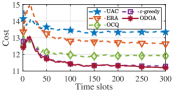
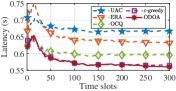
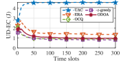
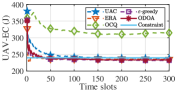
Figure 3: The impact of time slots on system performance. (a) Time-average IoTD cost (Cost). (b) Average task completion latency (Latency). (c) Time-average IoTD energy consumption (IoTD-EC). (d) Time-average UAV energy consumption (UAV-EC).

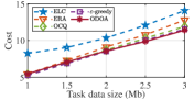
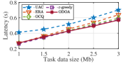
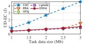
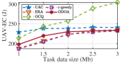
Figure 4: The impact of task data size on system performance. (a) Time-average IoTD cost (Cost). (b) Average task completion latency (Latency). (c) Time-average IoTD energy consumption (IoTD-EC). (d) Time-average UAV energy consumption (UAV-EC).

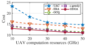
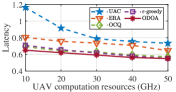
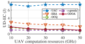
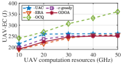
Figure 5: The impact of UAV computation resources on system performance. (a) Time-average IoTD cost (Cost). (b) Average task completion latency (Latency). (c) Time-average IoTD energy consumption (IoTD-EC). (d) Time-average UAV energy consumption (UAV-EC).

IV-B Evaluation Results

IV-B1 Impact of Time

Figs. 3(a), 3(b), 3(c) and 3(d) illustrate the dynamics of time-averaged IoTD cost, average task completion latency, time-averaged IoTD energy consumption, and time-averaged UAV energy consumption among the five approaches, respectively. OCQ achieves worse performance compared the proposed ODOA with respect to time-averaged IoTD cost, and average task completion latency. This is mainly due to the game-theoretic computation offloading algorithm. Specifically, regardless of the UAV energy constraint, more tasks are offloaded to the UAV, which leads to a decrease in the overall performance owing to the limited computing resources of the UAV. Moreover, the proposed ODOA outperforms UAC, ERA, and $\varepsilon$-greedy with respect to time-averaged IoTD cost and average task completion latency. The reasons are as follows. First, the three-tier architecture combined with cloud computing offers abundant resource supply. Second, the optimal resource allocation strategy can more effectively utilize the limited resources of the UAV. Third, the UCB-based algorithm better balances exploration and exploitation to enhance the accuracy of latency prediction. Finally, as shown in Fig. 3(d), the proposed ODOA can satisfy the long-term UAV energy constraint under the real-time guidance of the Lyapunov-based energy queue, which is consistent with the analysis in Theorem 8.

In conclusion, the set of simulation results demonstrates that the ODOA effectively improves overall performance while adhering to the UAV energy constraint.

IV-B2 Impact of Task Data Size

Figs. 4(a), 4(b), 4(c), and 4(d) show the impact of different task data sizes on various performance metrics. With the increase in task data sizes, there is an upward trend with respect to the time-averaged IoTD cost, average task completion latency, time-averaged IoTD energy consumption, and time-averaged UAV energy consumption. This is expected since the larger task data size leads to higher overheads on computing, communication, and energy consumption for both IoTDs and the UAV. In addition, UAC exhibits a significant growth trend with respect to the time-averaged IoTD cost and average task completion latency compared to the other approaches. This is because UAC relies heavily on the limited computing resources of the UAV, which becomes a bottleneck for system performance as the size of task data continues to increase. Finally, compared with UAC, ERA, OCQ and $\varepsilon$-greedy, the proposed ODOA exhibits superior performance with respect to time-averaged IoTD cost as the task data size increases, and achieves performance improvements of approximately 18.9%, 10.7%, 4.1%, and 1.2% with respect to average task completion latency when the task data size reaches 3 Mb.

In summary, the set of simulation results indicates that the proposed ODOA can effectively adapt to heavily loaded scenarios, delivering overall superior performance.

IV-B3 Impact of UAV Computation Resources

Figs. 5(a), 5(b), 5(c), and 5(d) compare the impact of different UAV computation resources on various performance metrics for the five approaches. It can be observed that with the increase of UAV computation resources, all approaches show a decreasing trend with respect to the time-averaged IoTD cost and average task completion latency. Moreover, UAC and ODOA demonstrate gradually decreasing performance improvements. The reasons are as follows. The increase of UAV computation resources provides more computing resource allocation for task execution, reducing the task execution latency. However, as UAV computation resources further increase, communication resources and the energy constraints of UAV become bottlenecks that limit the improvement of system performance. Furthermore, OCQ shows a significant upward trend in terms of time-averaged UAV energy consumption with the increase in UAV computation resources. This is mainly because OCQ does not take into account the energy consumption constraints of the UAV. Therefore, the increase in computing resources leads to more tasks being offloaded to the UAV for processing, which in turn increases its energy consumption.

Finally, ODOA outperforms UAC, ERA, OCQ, and $\varepsilon$-greedy with respect to the time-averaged IoTD cost and average task completion latency, which illustrates the proposed approach enables sustainable utilization of computing resources and prevents resource over-utilization.

V Conclusion

In this work, we explored the integration of computation offloading, satellite selection, resource allocation, and UAV trajectory control in an SAGIMEC-assisted ICPS. We formally formulated the optimization problem to maximize the QoS for all IoTDs. To solve this complex problem, we proposed ODOA, which combines the Lyapunov optimization framework for online control, the MAB model for online learning, and game theory for decentralized algorithm design. The mathematical analysis demonstrated that the ODOA not only meets the UAV energy constraint but also features low computational complexity. Simulation results indicated that the ODOA exhibits overall superior performance with respect to the time-averaged IoTD cost, average task completion latency, and time-averaged IoTD energy consumption.

References

- [1] K. Zhang, Y. Shi, S. Karnouskos, T. Sauter, H. Fang, and A. W. Colombo, “Advancements in industrial cyber-physical systems: An overview and perspectives,” IEEE Trans. Ind. Informatics, vol. 19, no. 1, pp. 716–729, Jan. 2023.
- [2] K. Cao, S. Hu, Y. Shi, A. W. Colombo, S. Karnouskos, and X. Li, “A survey on edge and edge-cloud computing assisted cyber-physical systems,” IEEE Trans. Ind. Informatics, vol. 17, no. 11, pp. 7806–7819, Nov. 2021.
- [3] S. Li, Q. Ni, Y. Sun, G. Min, and S. Al-Rubaye, “Energy-efficient resource allocation for industrial cyber-physical IoT systems in 5G era,” IEEE Trans. Ind. Informatics, vol. 14, no. 6, pp. 2618–2628, Jun. 2018.
- [4] Y. Hao, M. Chen, H. Gharavi, Y. Zhang, and K. Hwang, “Deep reinforcement learning for edge service placement in softwarized industrial cyber-physical system,” IEEE Trans. Ind. Informatics, vol. 17, no. 8, pp. 5552–5561, Aug. 2021.
- [5] K. Wang, J. Jin, Y. Yang, T. Zhang, A. Nallanathan, C. Tellambura, and B. Jabbari, “Task offloading with multi-tier computing resources in next generation wireless networks,” IEEE J. Sel. Areas Commun., vol. 41, no. 2, pp. 306–319, February 2023.
- [6] X. Cheng, F. Lyu, W. Quan, C. Zhou, H. He, W. Shi, and X. Shen, “Space/aerial-assisted computing offloading for IoT applications: A learning-based approach,” IEEE J. Sel. Areas Commun., vol. 37, no. 5, pp. 1117–1129, May 2019.
- [7] K. Fan, B. Feng, X. Zhang, and Q. Zhang, “Demand-driven task scheduling and resource allocation in space-air-ground integrated network: A deep reinforcement learning approach,” IEEE Trans. Wirel. Commun., pp. 1–1, Early Access, 2024, doi:10.1109/TWC.2024.3398199.
- [8] Z. Hu, F. Zeng, Z. Xiao, B. Fu, H. Jiang, H. Xiong, Y. Zhu, and M. Alazab, “Joint resources allocation and 3D trajectory optimization for UAV-enabled space-air-ground integrated networks,” IEEE Trans. Veh. Technol., vol. 72, no. 11, pp. 14 214–14 229, Nov. 2023.
- [9] R. Zhou, X. Wu, H. Tan, and R. Zhang, “Two time-scale joint service caching and task offloading for UAV-assisted mobile edge computing,” in Proc. IEEE INFOCOM, 2022, pp. 1189–1198.
- [10] J. Liu, X. Zhao, P. Qin, S. Geng, and S. Meng, “Joint dynamic task offloading and resource scheduling for WPT enabled space-air-ground power internet of things,” IEEE Trans. Netw. Sci. Eng., vol. 9, no. 2, pp. 660–677, Mar.-Apr. 2022.
- [11] Y. Mao, J. Zhang, and K. B. Letaief, “Dynamic computation offloading for mobile-edge computing with energy harvesting devices,” IEEE J. Sel. Areas Commun., vol. 34, no. 12, pp. 3590–3605, 2016.
- [12] H. Jiang, X. Dai, Z. Xiao, and A. Iyengar, “Joint task offloading and resource allocation for energy-constrained mobile edge computing,” IEEE Trans. Mob. Comput., vol. 22, no. 7, pp. 4000–4015, Jul. 2023.
- [13] B. Li, R. Yang, L. Liu, J. Wang, N. Zhang, and M. Dong, “Robust computation offloading and trajectory optimization for multi-UAV-assisted MEC: A multiagent DRL approach,” IEEE Internet Things J., vol. 11, no. 3, pp. 4775–4786, Feb. 2024.
- [14] X. Zhang, J. Liu, R. Zhang, Y. Huang, J. Tong, N. Xin, L. Liu, and Z. Xiong, “Energy-efficient computation peer offloading in satellite edge computing networks,” IEEE Trans. Mob. Comput., vol. 23, no. 4, pp. 3077–3091, Apr. 2024.
- [15] F. Song, H. Xing, X. Wang, S. Luo, P. Dai, Z. Xiao, and B. Zhao, “Evolutionary multi-objective reinforcement learning based trajectory control and task offloading in UAV-assisted mobile edge computing,” IEEE Trans. Mob. Comput., vol. 22, no. 12, pp. 7387–7405, Dec. 2023.
- [16] Y. Pan, C. Pan, K. Wang, H. Zhu, and J. Wang, “Cost minimization for cooperative computation framework in MEC networks,” IEEE Trans. Wirel. Commun., vol. 20, no. 6, pp. 3670–3684, Jun. 2021.
- [17] Z. Wei, Y. Cai, Z. Sun, D. W. K. Ng, J. Yuan, M. Zhou, and L. Sun, “Sum-rate maximization for IRS-assisted UAV OFDMA communication systems,” IEEE Trans. Wirel. Commun., vol. 20, no. 4, pp. 2530–2550, Apr. 2021.
- [18] L. Zhang, Z. Zhang, L. Min, C. Tang, H. Zhang, Y. Wang, and P. Cai, “Task offloading and trajectory control for UAV-assisted mobile edge computing using deep reinforcement learning,” IEEE Access, vol. 9, pp. 53 708–53 719, Apr. 2021.
- [19] G. Sun, X. Zheng, Z. Sun, Q. Wu, J. Li, Y. Liu, and V. C. M. Leung, “UAV-enabled secure communications via collaborative beamforming with imperfect eavesdropper information,” IEEE Trans. Mob. Comput., vol. 23, no. 4, pp. 3291–3308, Apr. 2024.
- [20] Y. Chen, K. Li, Y. Wu, J. Huang, and L. Zhao, “Energy efficient task offloading and resource allocation in air-ground integrated MEC systems: A distributed online approach,” IEEE Trans. Mob. Comput., pp. 1–14, Early Access, 2023, doi: 10.1109/TMC.2023.3346431.
- [21] C. Niephaus, M. Kretschmer, and G. Ghinea, “QoS provisioning in converged satellite and terrestrial networks: A survey of the state-of-the-art,” IEEE Commun. Surv. Tutorials, vol. 18, no. 4, pp. 2415–2441, Fourthquarter 2016.
- [22] X. Gao, J. Wang, X. Huang, Q. Leng, Z. Shao, and Y. Yang, “Energy-constrained online scheduling for satellite-terrestrial integrated networks,” IEEE Trans. Mob. Comput., vol. 22, no. 4, pp. 2163–2176, 2023.
- [23] Y. Zeng, J. Xu, and R. Zhang, “Energy minimization for wireless communication with rotary-wing UAV,” IEEE Trans. Wirel. Commun., vol. 18, no. 4, pp. 2329–2345, Apr. 2019.
- [24] H. Pan, Y. Liu, G. Sun, J. Fan, S. Liang, and C. Yuen, “Joint power and 3D trajectory optimization for UAV-enabled wireless powered communication networks with obstacles,” IEEE Trans. Commun., vol. 71, no. 4, pp. 2364–2380, Apr. 2023.
- [25] Z. Yang, S. Bi, and Y. A. Zhang, “Online trajectory and resource optimization for stochastic UAV-enabled MEC systems,” IEEE Trans. Wirel. Commun., vol. 21, no. 7, pp. 5629–5643, Jul. 2022.
- [26] Y. Chen, J. Zhao, Y. Wu, J. Huang, and X. Shen, “QoE-aware decentralized task offloading and resource allocation for end-edge-cloud systems: A game-theoretical approach,” IEEE Trans. Mob. Comput., vol. 23, no. 1, pp. 769–784, Jan. 2024.
- [27] Y. Ding, K. Li, C. Liu, and K. Li, “A potential game theoretic approach to computation offloading strategy optimization in end-edge-cloud computing,” IEEE Trans. Parallel Distributed Syst., vol. 33, no. 6, pp. 1503–1519, Jun. 2022.
- [28] S. Boyd, S. P. Boyd, and L. Vandenberghe, Convex optimization. Cambridge university press, 2004.
- [29] P. Belotti, C. Kirches, S. Leyffer, J. Linderoth, J. Luedtke, and A. Mahajan, “Mixed-integer nonlinear optimization,” Acta Numerica, vol. 22, pp. 1–131, Apr. 2013.
- [30] M. J. Neely, Stochastic Network Optimization with Application to Communication and Queueing Systems, ser. Synthesis Lect. Commun. Netw. Morgan & Claypool Publishers, 2010.
- [31] A. Slivkins, “Introduction to multi-armed bandits,” Found. Trends Mach. Learn., vol. 12, no. 1-2, pp. 1–286, Nov. 2019.
- [32] F. Li, J. Liu, and B. Ji, “Combinatorial sleeping bandits with fairness constraints,” IEEE Trans. Netw. Sci. Eng., vol. 7, no. 3, pp. 1799–1813, Jul.-Sept. 2020.
- [33] G. Cui, Q. He, X. Xia, F. Chen, F. Dong, H. Jin, and Y. Yang, “OL-EUA: Online user allocation for NOMA-based mobile edge computing,” IEEE Trans. Mob. Comput., vol. 22, no. 4, pp. 2295–2306, Apr. 2023.
- [34] X. Zhang, J. Zhang, J. Xiong, L. Zhou, and J. Wei, “Energy-efficient multi-UAV-enabled multiaccess edge computing incorporating NOMA,” IEEE Internet Things J., vol. 7, no. 6, pp. 5613–5627, Jun. 2020.
- [35] M. Grant and S. Boyd, “CVX: Matlab software for disciplined convex programming, version 2.1,” http://cvxr.com/cvx, Mar. 2014.
- [36] D. Monderer and L. S. Shapley, “Potential Games,” Games Econ. Behav., vol. 14, no. 1, pp. 124–143, 1996.
- [37] D. L. Quang, Y. H. Chew, and B. H. Soong, “Potential game theory,” Springer International Publishing, 2016.
- [38] L. Wang, K. Wang, C. Pan, W. Xu, N. Aslam, and A. Nallanathan, “Deep reinforcement learning based dynamic trajectory control for UAV-assisted mobile edge computing,” IEEE Trans. Mob. Comput., vol. 21, no. 10, pp. 3536–3550, Oct. 2022.
- [39] A. Al-Hourani, K. Sithamparanathan, and S. Lardner, “Optimal LAP altitude for maximum coverage,” IEEE Wirel. Commun. Lett., vol. 3, no. 6, pp. 569–572, Dec. 2014.
- [40] S. Josilo and G. Dán, “Selfish decentralized computation offloading for mobile cloud computing in dense wireless networks,” IEEE Trans. Mob. Comput., vol. 18, no. 1, pp. 207–220, Jan. 2019.
- [41] J. Vermorel and M. Mohri, “Multi-armed bandit algorithms and empirical evaluation,” in Proc. of Eur.Conf.Mach. Learn., Oct. 2005, pp. 437–448.