Hybrid deep additive neural networks

Gyu Min Kim and Jeong Min Jeon

Department of Statistics, Seoul National University, South Korea

Department of Data Science, Ewha Womans University, South Korea

Abstract: Traditional neural networks (multi-layer perceptrons) have become an important tool in data science due to their success across a wide range of tasks. However, their performance is sometimes unsatisfactory, and they often require a large number of parameters, primarily due to their reliance on the linear combination structure. Meanwhile, additive regression has been a popular alternative to linear regression in statistics. In this work, we introduce novel deep neural networks that incorporate the idea of additive regression. Our neural networks share architectural similarities with Kolmogorov-Arnold networks but are based on simpler yet flexible activation and basis functions. Additionally, we introduce several hybrid neural networks that combine this architecture with that of traditional neural networks. We derive their universal approximation properties and demonstrate their effectiveness through simulation studies and a real-data application. The numerical results indicate that our neural networks generally achieve better performance than traditional neural networks while using fewer parameters.

Keywords: Additive model, Basis expansion, Deep learning, Neural network

1 Introduction

Additive regression is a statistical modeling approach developed to capture nonlinear relationships between the responses and predictors without relying on strict assumptions on the form of these relationships. Instead of assuming a linear relationship, additive models allow the response variable to depend on the sum of smooth and potentially nonlinear functions of each predictor variable. There have been a number of methods to estimate additive models, such as methods based on kernel smoothing (e.g., Linton and Nielsen (1995), Opsomer and Ruppert (1997), Mammen et al. (1999), Jeon and Park (2020), Jeon et al. (2022)) and methods based on basis expansions (e.g., Bilodeau (1992), Meier et al. (2009), Sardy and Ma (2024)).

On the other hand, neural networks are becoming an important method in regression analysis. Its good practical performance and nice theoretical properties have been investigated by numerous works (e.g., LeCun et al. (2015), Schmidhuber (2015), Bauer and Kohler (2019), Schmidt-Hieber (2020), Kohler and Langer (2021)). However, traditional neural networks (multi-layer perceptrons) sometimes struggle with capturing complex nonlinear relationships between predictors and responses. Additionally, they often require a huge number of parameters, which leads to high computational and memory demands. These issues mainly come from that each node does not have sufficient nonlinearity.

Recently, several modifications using nonlinear basis functions have been proposed to overcome this issue. For example, Fakhoury et al. (2022) proposed an approach that uses a B-spline basis expansion, instead of the composition of an activation function and an affine function, to construct each node. However, this work considered only one hidden layer. Horowitz and Mammen (2007) introduced a deep version of this neural network and suggested to use B-splines or smoothing splines to estimate their neural network. However, this work mainly focused on deriving asymptotic error rates with arbitrary estimators satisfying certain conditions. Recently, Liu et al. (2024) proposed Kolmogorov-Arnold networks that have the same architecture as Horowitz and Mammen (2007). This approach uses a linear combination of the sigmoid linear unit function and a B-spline basis expansion to form each node. Although Liu et al. (2024) demonstrates fair performance, it requires high computational cost, resulting in a long training time. Additionally, it is complicated to implement and is prone to overfitting. Moreover, its universal approximation theorem holds only for a certain class of smooth functions.

In this work, we propose an alternative approach to Liu et al. (2024). Specifically,

  • $\bullet$

    We propose a deep neural network that uses fixed activation functions and simple yet flexible basis functions, which make computation and implementation easy.

  • $\bullet$

    We introduce hybrid neural networks that combine the above neural network and the traditional neural networks, which effectively avoid overfitting.

  • $\bullet$

    We derive their universal approximation properties that hold for any continuous functions.

This paper is organized as follows. In Section 2, we introduce a neural network, named as a deep additive neural network (DANN), and its property. We also introduce its hybrid variants in Section 3. Section 4 contains simulation studies and Section 5 presents real data analysis. These numerical studies show that our neural networks have better performance than the traditional neural networks in terms of both prediction errors and numbers of parameters. Section 6 contains conclusions, and all technical proofs are provided in the Appendix.

2 Deep Additive Neural Networks

Let $Y\in\mathbb{R}$ be a response and $\mathbf{X}=(X_{1},\ldots,X_{d})^{\mathstrut\scriptscriptstyle{\top}}\in[0,1]^{d}$ for $d\geq 1$ be a vector of predictors. The traditional neural networks with single hidden layer assume that

(2.1) $\displaystyle{\rm E}(Y|\mathbf{X})=\sum_{k=1}^{p}w_{k}\sigma\left(\sum_{j=1}^{d}w_{jk}X_{j}+b_{k}\right),$

where $p\geq 1$ is the number of nodes in the hidden layer, $\sigma:\mathbb{R}\rightarrow\mathbb{R}$ is a non-polynomial continuous function, called an activation function, and $w_{k},w_{jk},b_{k}\in\mathbb{R}$ are parameters. The well-known universal approximation theorem (Cybenko (1989)) tells that, for any given continuous function $f:[0,1]^{d}\rightarrow\mathbb{R}$ and constant $\epsilon>0$, there exist $p\geq 1$ and $w_{k},w_{jk},b_{k}\in\mathbb{R}$ such that

$\displaystyle\sup_{\mathbf{x}=(x_{1},\ldots,x_{d})^{\mathstrut\scriptscriptstyle{\top}}\in[0,1]^{d}}\left|f(\mathbf{x})-\sum_{k=1}^{p}w_{k}\sigma\left(\sum_{j=1}^{d}w_{jk}x_{j}+b_{k}\right)\right|<\epsilon.$

In spite of this nice property, it has been known that the practical performance of (2.1) is not good enough, particularly when the target regression function ${\rm E}(Y|\mathbf{X}=\cdot)$ is highly nonlinear, because $\sigma$ is the only nonlinear function in (2.1).

To overcome this issue, we may replace the linear functions in (2.1) by nonlinear functions. Specifically, we consider the model

(2.2) $\displaystyle{\rm E}(Y|\mathbf{X})=\sum_{k=1}^{p}f_{k}\left(\sum_{j=1}^{d}f_{jk}(X_{j})\right),$

where $f_{k}:\mathbb{R}\rightarrow\mathbb{R}$ and $f_{jk}:[0,1]\rightarrow\mathbb{R}$ are possibly nonlinear functions. When $p=1$ and $f_{1}$ is the identity function, this model reduces to the standard additive model. By taking appropriate $f_{k}$ and $f_{jk}$, (2.2) may approximate highly nonlinear ${\rm E}(Y|\mathbf{X}=\cdot)$ better than (2.1) in practice. In fact, Kolmogorov’s superposition theorem (Kolmogorov (1957)) says that any continuous function $f:[0,1]^{d}\rightarrow\mathbb{R}$ can be written as $\sum_{k=1}^{p}\phi^{f}_{k}(\sum_{j=1}^{d}\phi^{f}_{jk}(x_{j}))$ for some $p\geq 1$ and continuous functions $\phi^{f}_{k}:\mathbb{R}\rightarrow\mathbb{R}$ and $\phi^{f}_{jk}:[0,1]\rightarrow\mathbb{R}$. In this work, we take $f_{k}$ and $f_{jk}$ that can well approximate unknown $\phi^{m}_{k}$ and $\phi^{m}_{jk}$, where $m:={\rm E}(Y|\mathbf{X}=\cdot)$. For this, we introduce a lemma.

Refer to caption
Refer to caption
Figure 1: Architectures of (2.1) (left) and (2.2) (right). In the left panel, $W_{k}$ denotes $(w_{1k},\ldots,w_{dk})^{\mathstrut\scriptscriptstyle{\top}}\in\mathbb{R}^{d}$.
Lemma 1.

There exists a set $\{B_{r}:[0,1]\rightarrow\mathbb{R}\,|\,r\geq 1\}$ of known functions such that, for any given continuous function $\phi:[0,1]\rightarrow\mathbb{R}$ and constant $\epsilon>0$, there exist $q\geq 1$ and $c_{r},c\in\mathbb{R}$ such that

$\displaystyle\sup_{x\in[0,1]}\left|\phi(x)-\left(\sum_{r=1}^{q}c_{r}B_{r}(x)+c\right)\right|<\epsilon.$

For example, $\{B_{r}(x):r\geq 1\}=\{x^{r}:r\geq 1\}$, $\{B_{r}(x):r\geq 1\}=\{\cos(r\pi x):r\geq 1\}$ and the Haar system on $[0,1]$ (e.g., Haar (1910)), among many others, have the above property; see the proof of Lemma 1. In this work, we call $B_{r}$ satisfying the property of Lemma 1 basis functions. From this,

$\displaystyle\sum_{j=1}^{d}\phi^{m}_{jk}(x_{j})$

can be well approximated by

$\displaystyle\sum_{j=1}^{d}\sum_{r=1}^{q_{jk}}c_{jkr}B_{jkr}(x_{j})+b_{k}$

for some $q_{jk}\geq 1$ and $c_{jkr},b_{k}\in\mathbb{R}$, and any possibly different sets $\{B_{1kr}:r\geq 1\},\ldots,\{B_{dkr}:r\geq 1\}$ of basis functions. We also approximate $\phi^{m}_{k}:\mathbb{R}\rightarrow\mathbb{R}$ by the function

$\displaystyle\sum_{\ell=1}^{q_{k}}c_{k\ell}B_{k\ell}(g(\cdot))+b,$

where $q_{k}\geq 1$, $c_{k\ell},b\in\mathbb{R}$, $\{B_{k\ell}:\ell\geq 1\}$ is a set of basis functions, and $g:\mathbb{R}\rightarrow[0,1]$ is a function. We call the model

(2.3) $\displaystyle{\rm E}(Y|\mathbf{X})=\sum_{k=1}^{p}\sum_{\ell=1}^{q_{k}}c_{k\ell}B_{k\ell}\left(g\left(\sum_{j=1}^{d}\sum_{r=1}^{q_{jk}}c_{jkr}B_{jkr}(X_{j})+b_{k}\right)\right)+b$

an Additive Neural Network (ANN). Figure 2 illustrates the architecture of ANN. The following theorem shows that the ANN is a reasonable model.

Refer to caption
Figure 2: Architecture of ANN model.
Theorem 1.

Let $\{B_{k\ell}:\ell\geq 1\}$ and $\{B_{jkr}:r\geq 1\}$ be any sets of basis functions and $g$ be non-constant and Lipschitz continuous. Then, for any given continuous function $f:[0,1]^{d}\rightarrow\mathbb{R}$ and constant $\epsilon>0$, there exist $p,q_{k},q_{jk}\geq 1$ and $c_{k\ell},c_{jkr},b_{k},b\in\mathbb{R}$ such that

$\displaystyle\sup_{\mathbf{x}\in[0,1]^{d}}\left|f(\mathbf{x})-\left(\sum_{k=1}^{p}\sum_{\ell=1}^{q_{k}}c_{k\ell}B_{k\ell}\left(g\left(\sum_{j=1}^{d}\sum_{r=1}^{q_{jk}}c_{jkr}B_{jkr}(x_{j})+b_{k}\right)\right)+b\right)\right|<\epsilon.$

Examples of $g$ satisfying the assumption in Theorem 1 include the logistic function, $(\rm{tanh}+1)/2$ and any Lipschitz continuous cumulative distribution function, where tanh is the hyperbolic tangent function. The hyperparameters of ANN that we need to choose include $p$, $q_{k}$, $q_{jk}$, $g$ and the sets of basis functions. For given hyperparameters, we estimate $c_{k\ell}$, $c_{jkr}$, $b_{k}$ and $b$ in (2.3) by finding values that minimize $\sum_{i=1}^{n}(Y_{i}-\hat{Y}_{i})^{2}$. For this, we initialize them and then update subsequently using an optimization algorithm.

Remark 1.

The ANN has important advantages.

  • 1.

    First, the ANN architecture is easy to build. Note that $\{B_{jkr}(X_{j}):1\leq j\leq d,1\leq r\leq q_{jk}\}$ for $1\leq k\leq p$ that are in the left rectangles of Figure 2 can be easily obtained from $\mathbf{X}$. Similarly, $\{B_{k\ell}(g(\sum_{j=1}^{d}\sum_{r=1}^{q_{jk}}c_{jkr}B_{jkr}(X_{j})+b_{k})):1\leq\ell\leq q_{k}\}$ that is in the $k$th right rectangle of Figure 2 can be easily obtained from $g(\sum_{j=1}^{d}\sum_{r=1}^{q_{jk}}c_{jkr}B_{jkr}(X_{j})+b_{k})$ for $1\leq k\leq p$. If we use the same basis set, say $\{B_{r}:r\geq 1\}$, and the same number of basis functions, say $q$, across all nodes, then the ANN architecture is even more simplified; see Figure 3.

  • 2.

    Second, we can directly apply optimization algorithms used for the traditional neural networks, such as ADAM (Kingma and Ba (2017)), to update the parameters of ANN. This is because $\sum_{j=1}^{d}\sum_{r=1}^{q_{jk}}c_{jkr}B_{jkr}(X_{j})+b_{k}$ is simply the linear combination of $\{B_{jkr}(X_{j}):1\leq j\leq d,1\leq r\leq q_{jk}\}\cup\{1\}$ for $1\leq k\leq p$, and

    $\displaystyle\sum_{k=1}^{p}\sum_{\ell=1}^{q_{k}}c_{k\ell}B_{k\ell}\left(g\left(\sum_{j=1}^{d}\sum_{r=1}^{q_{jk}}c_{jkr}B_{jkr}(X_{j})+b_{k}\right)\right)+b$

    is simply the linear combination of $\{B_{k\ell}(g(\sum_{j=1}^{d}\sum_{r=1}^{q_{jk}}c_{jkr}B_{jkr}(X_{j})+b_{k})):1\leq k\leq p,1\leq\ell\leq q_{k}\}\cup\{1\}$.

  • 3.

    Cosine basis might approximate a periodic function well and the Haar basis might approximate a non-smooth function well. By mixing various types of basis, the ANN might approximate diverse functions well in practice.

Refer to caption
Figure 3: Architecture of ANN model in the case of the same set and same number of basis functions.

It has been known that the traditional neural networks with multiple hidden layers, sometimes called a Deep Neural Network (DNN), tends to provide better performance than that with single hidden layer. This motivates us to add more hidden layers to the ANN. The ANN with $L$ hidden layers is illustrated in Figure 4. Formally, it can be written as

(2.4) $\displaystyle\begin{split}{\rm E}(Y|\mathbf{X})&=\sum_{k=1}^{p_{L}}\sum_{r=1}^{q_{k}}c_{kr}B_{kr}(X_{k}^{(L)})+b,\\ X_{k}^{(L)}&=g_{L}\left(\sum_{j=1}^{p_{L-1}}\sum_{r=1}^{q_{jk}^{(L)}}c_{jkr}^{(L)}B_{jkr}^{(L)}\left(X_{j}^{(L-1)}\right)+b_{k}^{(L)}\right)\text{ for }k=1,\ldots,p_{L},\\ &\vdots\\ X_{k}^{(1)}&=g_{1}\left(\sum_{j=1}^{d}\sum_{r=1}^{q_{jk}^{(1)}}c_{jkr}^{(1)}B_{jkr}^{(1)}(X_{j})+b_{k}^{(1)}\right)\text{ for }k=1,\ldots,p_{1},\end{split}$

where $p_{l}$ is the number of nodes in the $l$th hidden layer, $\{B_{kr}:r\geq 1\}$ and $\{B_{jkr}^{(l)}:r\geq 1\}$ are sets of basis functions, $q_{k}$ and $q_{jk}^{(l)}$ are the numbers of used basis functions, $g_{l}:\mathbb{R}\rightarrow[0,1]$ are functions, and $c_{kr},c_{jkr}^{(l)},b_{k}^{(l)},b\in\mathbb{R}$ are parameters. We call (2.4) a Deep Additive Neural Network (DANN).

Refer to caption
Figure 4: Architecture of DANN model.

The advantages of ANN given in Remark 1 are still valid for the DANN. In particular, constructing basis functions in this network is easier than that in Liu et al. (2024) since the output values from $g_{l}$ lie in $[0,1]$, and hence we do not need to adapt basis functions in the next layer according to the output values. In Liu et al. (2024), however, knots for the B-spline basis need to be adjusted according to the output values from their activation functions.

3 Hybrid Networks

The DANN may approximate a complex regression function well, but its complexity might be too high for a relatively simple regression function. In the latter case, it can overfit data. To adjust the model complexity, we introduce three networks that combine the architectures of ANN and DNN. These networks use the architecture of ANN for some layers and use that of DNN for other layers.

The first hybrid network, namely the Hybrid Deep Additive Neural Network 1 (HDANN1), uses the ANN architecture to construct the first hidden layer and uses the DNN architecture for the remaining layers. This network is illustrated in Figure 5. Formally, it can be written as

(3.5) $\displaystyle\begin{split}{\rm E}(Y|\mathbf{X})&=\sum_{k=1}^{p_{L}}w_{k}X_{k}^{(L)}+b,\\ X_{k}^{(L)}&=\sigma_{L}\left({W_{k}^{(L)}}^{\mathstrut\scriptscriptstyle{\top}}\mathbf{X}^{(L-1)}+b_{k}^{(L)}\right)\text{ for }k=1,\ldots,p_{L},\\ &\vdots\\ X_{k}^{(2)}&=\sigma_{2}\left({W_{k}^{(2)}}^{\mathstrut\scriptscriptstyle{\top}}\mathbf{X}^{(1)}+b_{k}^{(2)}\right)\text{ for }k=1,\ldots,p_{2},\\ X_{k}^{(1)}&=\sigma_{1}\left(\sum_{j=1}^{d}\sum_{r=1}^{q_{jk}}c_{jkr}B_{jkr}(X_{j})+b_{k}^{(1)}\right)\text{ for }k=1,\ldots,p_{1},\end{split}$

where $W_{k}^{(l)}\in\mathbb{R}^{p_{l-1}}$ are vectors of weight parameters, $\mathbf{X}^{(l)}=\big{(}X_{1}^{(l)},\ldots,X_{p_{l}}^{(l)}\big{)}^{\mathstrut\scriptscriptstyle{\top}}\in\mathbb{R}^{p_{l}}$, and $\sigma_{l}:\mathbb{R}\rightarrow\mathbb{R}$ are functions.

Refer to caption
Figure 5: Architecture of HDANN1 model.

This network also has the universal approximation property even when $p_{1}=\cdots=p_{L}$ and $\sigma_{1}=\cdots=\sigma_{L}$. To describe this, let $\mathbf{q}$ denote the collection of $q_{jk}$, $\mathbf{W}$ denote the collection of $W_{k}^{(l)}$, $\mathbf{c}$ denote the collection of $c_{jkr}$, and $\mathbf{b}$ denote the collection of $b_{k}^{(l)}$ and $b$. Also, let

$\displaystyle{\rm HDANN}1_{L,\mathbf{q},\mathbf{W},\mathbf{c},\mathbf{b}}(\mathbf{x})=\sum_{k=1}^{p_{L}}w_{k}x_{k}^{(L)}+b$

denote the function on $[0,1]^{d}$ defined through the architecture at (3.5).

Theorem 2.

Let $\{B_{jkr}:r\geq 1\}$ be any sets of basis functions, $p_{1}=\cdots=p_{L}$, and $\sigma_{1}=\cdots=\sigma_{L}$ be a non-affine Lipschitz continuous function which is continuously differentiable at at least one point, with nonzero derivative at that point. Then, for any given continuous function $f:[0,1]^{d}\rightarrow\mathbb{R}$ and constant $\epsilon>0$, there exist $L,q_{jk}\geq 1$, $W_{k}^{(l)}\in\mathbb{R}^{p_{l-1}}$ and $c_{jkr},b_{k}^{(l)},b\in\mathbb{R}$ such that

$\displaystyle\sup_{\mathbf{x}\in[0,1]^{d}}\left|f(\mathbf{x})-{\rm HDANN}1_{L,\mathbf{q},\mathbf{W},\mathbf{c},\mathbf{b}}(\mathbf{x})\right|<\epsilon.$

Examples of $\sigma_{l}$ satisfying the assumption in Theorem 2 include the logistic function, the rectified linear unit (ReLU) function and tanh.

The second hybrid network, namely the Hybrid Deep Additive Neural Network 2 (HDANN2), is the reverse version of HDANN1. It adopts the ANN architecture to construct the output layer and the DNN architecture for the hidden layers. This network is written below and visualized in Figure 6.

(3.6) $\displaystyle\begin{split}{\rm E}(Y|\mathbf{X})&=\sum_{k=1}^{p_{L}}\sum_{r=1}^{q_{k}}c_{kr}B_{kr}(X_{k}^{(L)})+b,\\ X_{k}^{(L)}&=g_{L}\left({W_{k}^{(L)}}^{\mathstrut\scriptscriptstyle{\top}}\mathbf{X}^{(L-1)}+b_{k}^{(L)}\right)\text{ for }k=1,\ldots,p_{L},\\ X_{k}^{(L-1)}&=\sigma_{L-1}\left({W_{k}^{(L-1)}}^{\mathstrut\scriptscriptstyle{\top}}\mathbf{X}^{(L-2)}+b_{k}^{(L-1)}\right)\text{ for }k=1,\ldots,p_{L-1},\\ &\vdots\\ X_{k}^{(1)}&=\sigma_{1}\left({W_{k}^{(1)}}^{\mathstrut\scriptscriptstyle{\top}}\mathbf{X}+b_{k}^{(1)}\right)\text{ for }k=1,\ldots,p_{1},\end{split}$

where $g_{L}:\mathbb{R}\rightarrow[0,1]$ and $\sigma_{l}:\mathbb{R}\rightarrow\mathbb{R}$ are functions.

Refer to caption
Figure 6: Architecture of HDANN2 model.

This network also has the universal approximation property even when $p_{1}=\cdots=p_{L}$ and $\sigma_{1}=\cdots=\sigma_{L-1}=g_{L}$. Define $\mathbf{q},\mathbf{W},\mathbf{c}$ and $\mathbf{b}$ similarly as in the case of HDANN1 and let

$\displaystyle{\rm HDANN}2_{L,\mathbf{q},\mathbf{W},\mathbf{c},\mathbf{b}}(\mathbf{x})=\sum_{k=1}^{p_{L}}\sum_{r=1}^{q_{k}}c_{kr}B_{kr}(x_{k}^{(L)})+b$

denote the function on $[0,1]^{d}$ defined through the architecture at (3.6).

Theorem 3.

Let $\{B_{kr}:r\geq 1\}$ be any sets of basis functions, $p_{1}=\cdots=p_{L}$, and $\sigma_{1}=\cdots=\sigma_{L-1}=g_{L}$ be a continuous function which is continuously differentiable at at least one point, with nonzero derivative at that point. Then, for any given continuous function $f:[0,1]^{d}\rightarrow\mathbb{R}$ and constant $\epsilon>0$, there exist $L,q_{k}\geq 1$, $W_{k}^{(l)}\in\mathbb{R}^{p_{l-1}}$ and $c_{kr},b_{k}^{(l)},b\in\mathbb{R}$ such that

$\displaystyle\sup_{\mathbf{x}\in[0,1]^{d}}\left|f(\mathbf{x})-{\rm HDANN}2_{L,\mathbf{q},\mathbf{W},\mathbf{c},\mathbf{b}}(\mathbf{x})\right|<\epsilon.$

The third hybrid network, namely the Hybrid Deep Additive Neural Network 3 (HDANN3), combines the HDANN1 and HDANN2. This network takes the ANN architecture for the first hidden layer and output layer and takes the DNN architecture for the remaining layers. This network is formulated below and depicted in Figure 7.

(3.7) $\displaystyle\begin{split}{\rm E}(Y|\mathbf{X})&=\sum_{k=1}^{p_{L}}\sum_{r=1}^{q_{k}}c_{kr}B_{kr}(X_{k}^{(L)})+b,\\ X_{k}^{(L)}&=g_{L}\left({W_{k}^{(L)}}^{\mathstrut\scriptscriptstyle{\top}}\mathbf{X}^{(L-1)}+b_{k}^{(L)}\right)\text{ for }k=1,\ldots,p_{L},\\ X_{k}^{(L-1)}&=\sigma_{L-1}\left({W_{k}^{(L-1)}}^{\mathstrut\scriptscriptstyle{\top}}\mathbf{X}^{(L-2)}+b_{k}^{(L-1)}\right)\text{ for }k=1,\ldots,p_{L-1},\\ &\vdots\\ X_{k}^{(2)}&=\sigma_{2}\left({W_{k}^{(2)}}^{\mathstrut\scriptscriptstyle{\top}}\mathbf{X}^{(1)}+b_{k}^{(2)}\right)\text{ for }k=1,\ldots,p_{2},\\ X_{k}^{(1)}&=\sigma_{1}\left(\sum_{j=1}^{d}\sum_{r=1}^{q_{jk}}c_{jkr}B_{jkr}(X_{j})+b_{k}^{(1)}\right)\text{ for }k=1,\ldots,p_{1}.\end{split}$
Refer to caption
Figure 7: Architecture of HDANN3 model.

Note that the HDANN3 reduces to the ANN, which already has the universal approximation property, when there is a single hidden layer ($L=1$).

4 Simulations

In this section, we compare the proposed networks (DANN, HDANN1, HDANN2 and HDANN3) with the DNN. We compare not only their prediction performance but also the numbers of parameters. We generated $Y$ from the following two models:

(4.8) $\displaystyle\begin{split}\text{Model 1: }Y&=\exp\left(\sum_{j=1}^{3}X_{j}^{3}-\sum_{j=4}^{6}X_{j}^{3}\right)+\varepsilon,\\ \text{Model 2: }Y&=\left(1+X_{1}+2X_{2}^{2}+3X_{3}^{3}-\exp(X_{4})-\log(X_{5}+1)-\left|X_{6}-0.5\right|\right)^{2}+\varepsilon,\end{split}$

where $X_{j}$ were generated from the uniform distribution $U(0,1)$ and the error term $\varepsilon$ was generated from the normal distribution $N(0,0.1^{2})$ independently of $\mathbf{X}$.

To reduce the number of hyperparameter combinations, we used the same number of nodes and the same activation function across all hidden layers, that is, $p_{l}\overset{l}{\equiv}p$ and $\sigma_{l}\overset{l}{\equiv}\sigma$. For the DNN, we explored all combinations of $L\in\{2\times t:1\leq t\leq 9\}$, $p\in\{2^{t}:t=3,5,7,9,11\}$ and $\sigma\in\{\text{logistic, ReLU, tanh}\}$. This resulted in $9\times 5\times 3=135$ combinations for the DNN. For the proposed networks, we used the logistic function for all $g_{l}$. We also used the same set $\{B_{r}:r\geq 1\}$ of basis functions and the same number $q$ of basis functions across all layers and nodes. We investigated all combinations of $L\in\{1,3,5,7,9\}$, $p\in\{2^{t}:t=2,4,6,8,10\}$, $q\in\{3,5,7,9,11\}$ and $\sigma\in\{\text{logistic, ReLU, tanh}\}$, along with two basis options, $\{B_{r}(x):r\geq 1\}=\{x^{r}:r\geq 1\}$ (polynomial) and $\{B_{r}(x):r\geq 1\}=\{\cos(r\pi x):r\geq 1\}$ (cosine). This resulted in $5\times 5\times 5\times 3\times 2=750$ combinations for each proposed network.

In this setting, the number of parameters for each network is given by

$\displaystyle\#\text{DNN}(d,L,p)$ $\displaystyle=(d+1)p+(p+1)p(L-1)+p+1,$
$\displaystyle\#\text{DANN}(d,L,p,q)$ $\displaystyle=(dq+1)p+(pq+1)p(L-1)+pq+1,$
$\displaystyle\#\text{HDANN1}(d,L,p,q)$ $\displaystyle=(dq+1)p+(p+1)p(L-1)+p+1,$
$\displaystyle\#\text{HDANN2}(d,L,p,q)$ $\displaystyle=(d+1)p+(p+1)p(L-1)+pq+1,$
$\displaystyle\#\text{HDANN3}(d,L,p,q)$ $\displaystyle=(dq+1)p+(p+1)p(L-1)+pq+1.$

With the largest $L,p$ and $q$ for each network, it holds that

$\displaystyle\#\text{DANN}(6,9,2^{10},11)>\#\text{DNN}(6,18,2^{11})$
$\displaystyle>\#\text{HDANN3}(6,9,2^{10},11)>\#\text{HDANN1}(6,9,2^{10},11)>\#\text{HDANN2}(6,9,2^{10},11).$

For each model in (4.8), we generated three sets of samples, a training set, a validation set and a test set. The sample sizes of the latter two sets were fixed at 500, while the size of the training set was either 1000 (scenario 1) or 2000 (scenario 2). In the training process, we used standardized response values $Y^{\rm st}_{i}$. Here, the mean and standard deviation for the standardization were computed from the training set. The parameters were initialized using the Xavier uniform initialization (Glorot and Bengio (2010)) and then updated in the direction of minimizing $\sum_{i\in I_{\rm train}}(Y^{\rm st}_{i}-\hat{Y}^{\rm st}_{i})^{2}$ using the ADAM optimization with a batch size of 512 and a learning rate of $10^{-4}$, where $I_{{\rm train}}$ is the index set of the training set. To reduce computation time, we ceased the updating process if $\sum_{i\in I_{\rm train}}(Y^{\rm st}_{i}-\hat{Y}^{\rm st}_{i})^{2}/|I_{\rm train}|$ did not decrease by more than $10^{-3}$ over the recent 10 updates.

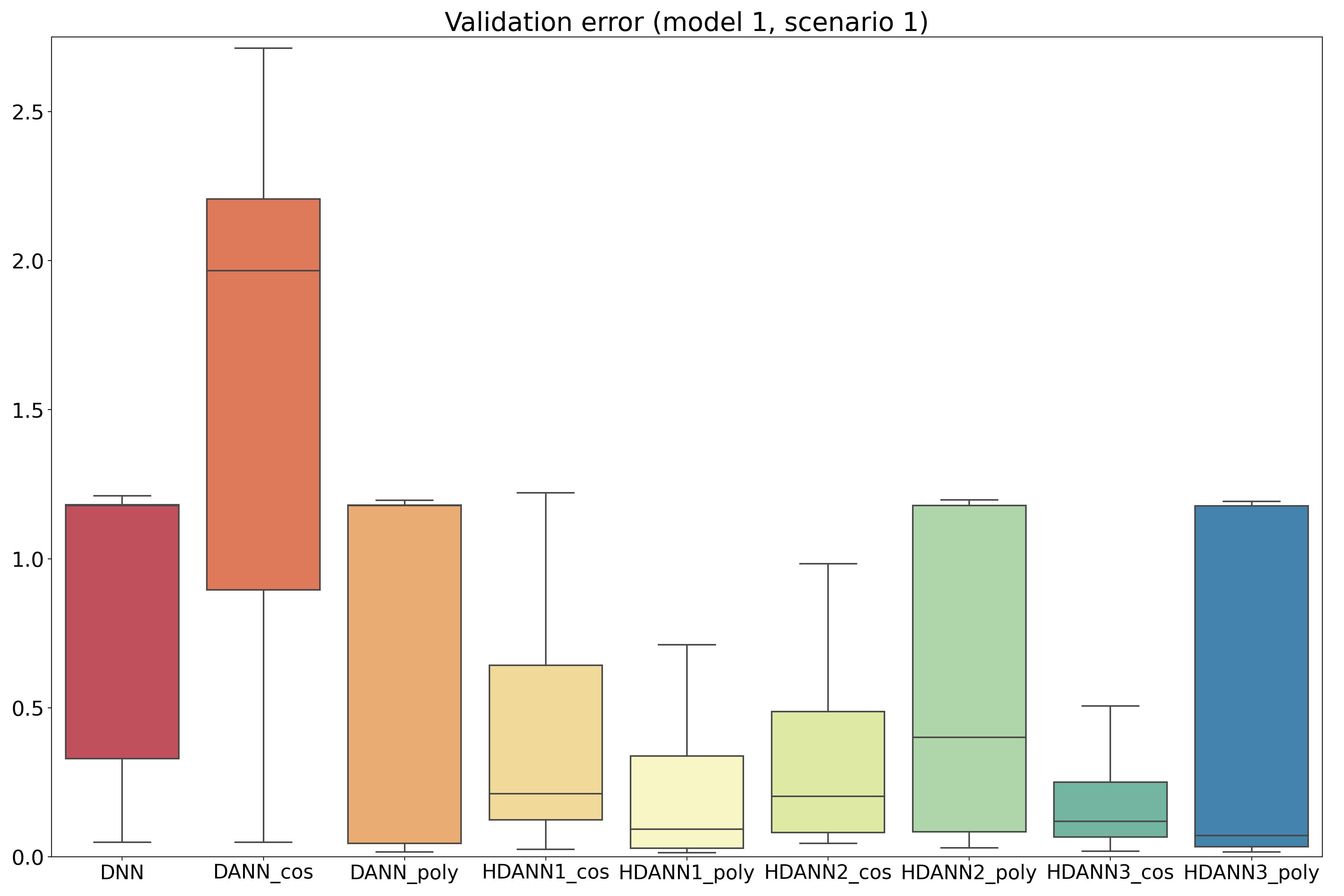
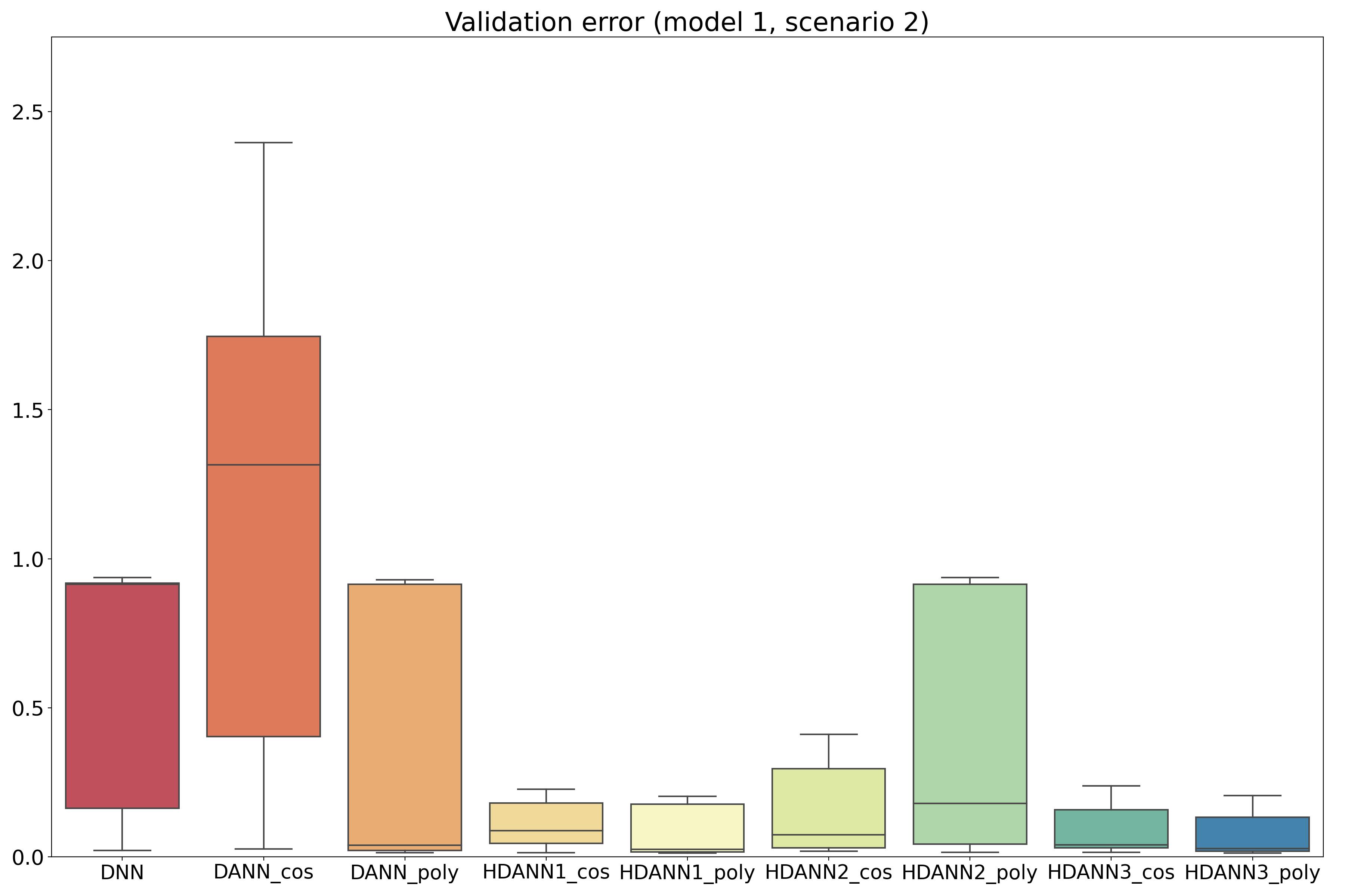
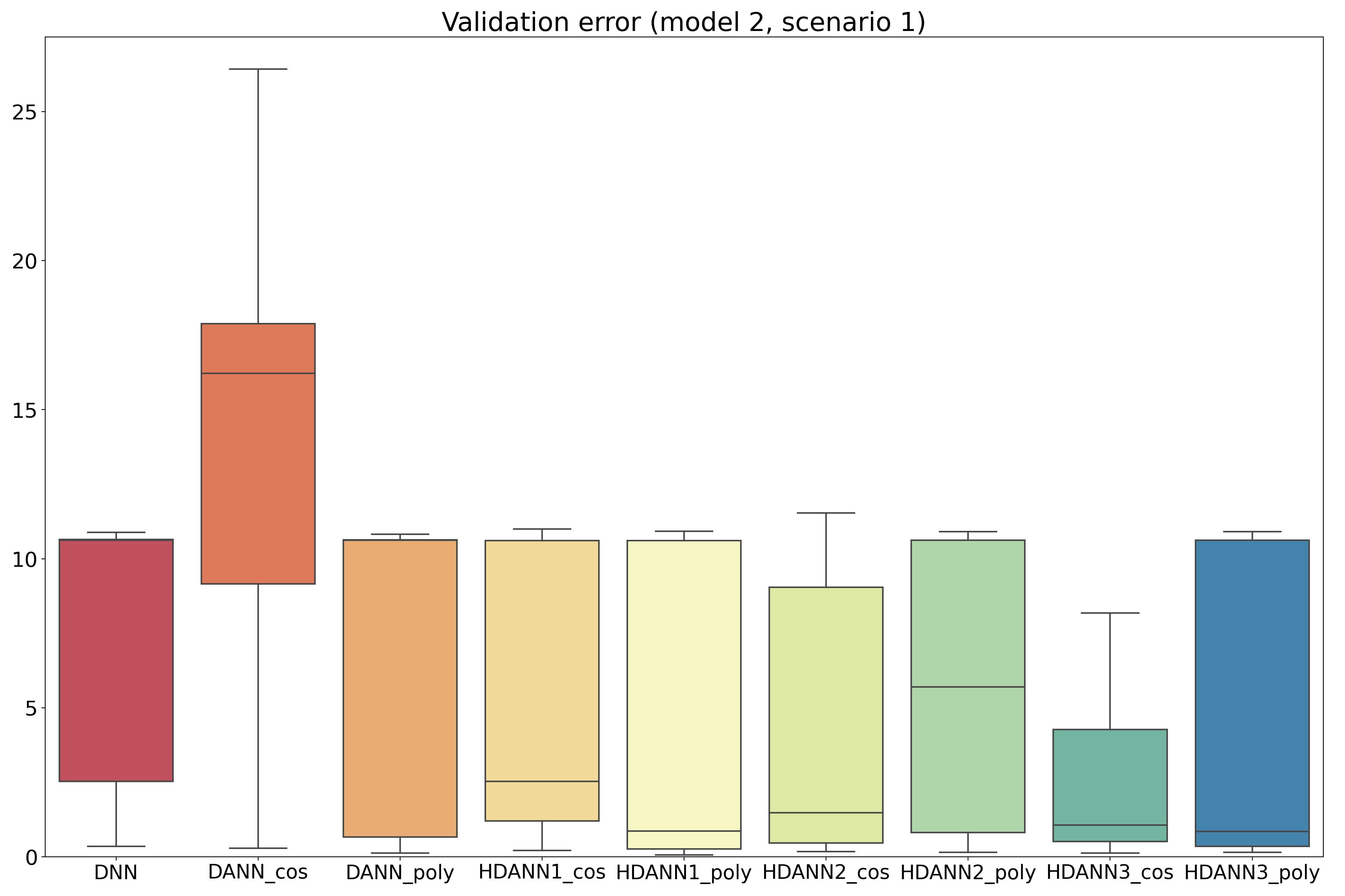
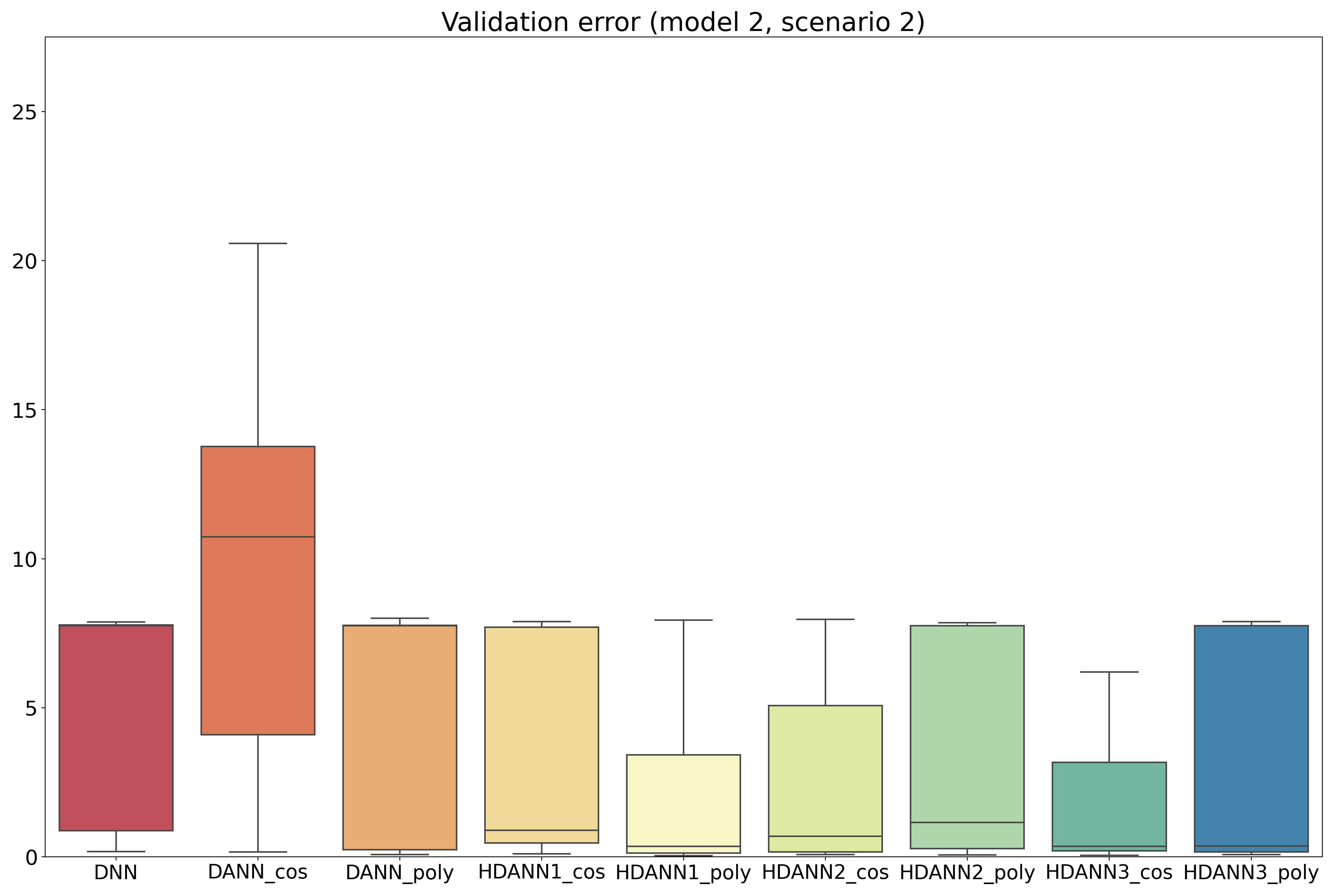
After training the networks, we evaluated the validation errors in the original response scale. Figure 8 displays the boxplot of $\sum_{i\in I_{\rm validation}}(Y_{i}-\hat{Y}_{i})^{2}/500$ across all hyperparameter combinations for each network. We separated boxplots for different basis types to see their effects. This figure shows that the DANN with cosine basis generally yields higher validation errors compared to the DNN, while the other proposed networks tend to have lower validation errors than the DNN. This figure also reveals that the polynomial basis generally yields better performance than the cosine basis for the DANN and HDANN1, while the opposite trend holds for the HDANN2 and HDANN3.

Refer to caption
Refer to caption
Refer to caption
Refer to caption
Figure 8: Boxplots of $\sum_{i\in I_{\rm validation}}(Y_{i}-\hat{Y}_{i})^{2}/500$. Each of the DNN and $\rm{DANN_{poly}}$ for model 1 in scenario 1 and for model 2 has almost the same median and Q3 values.

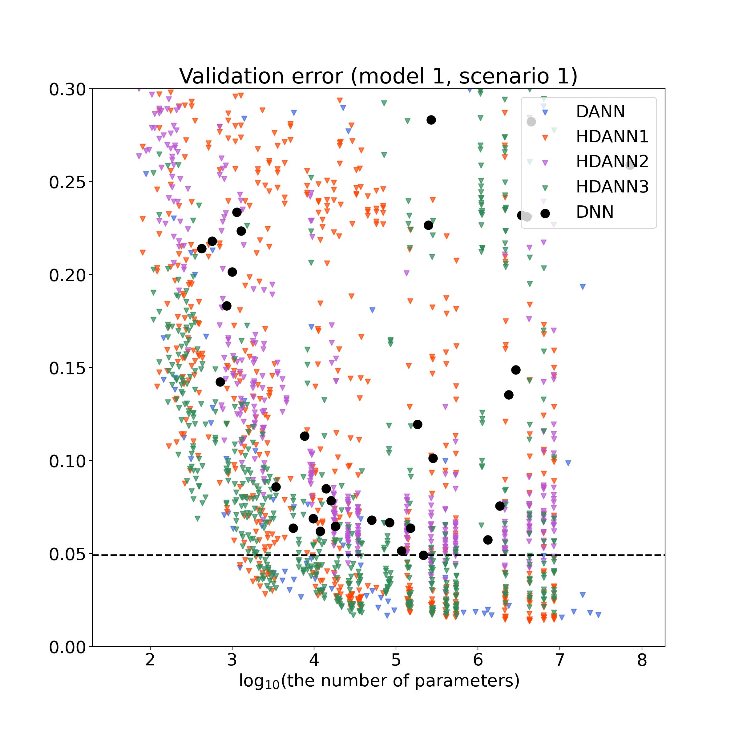
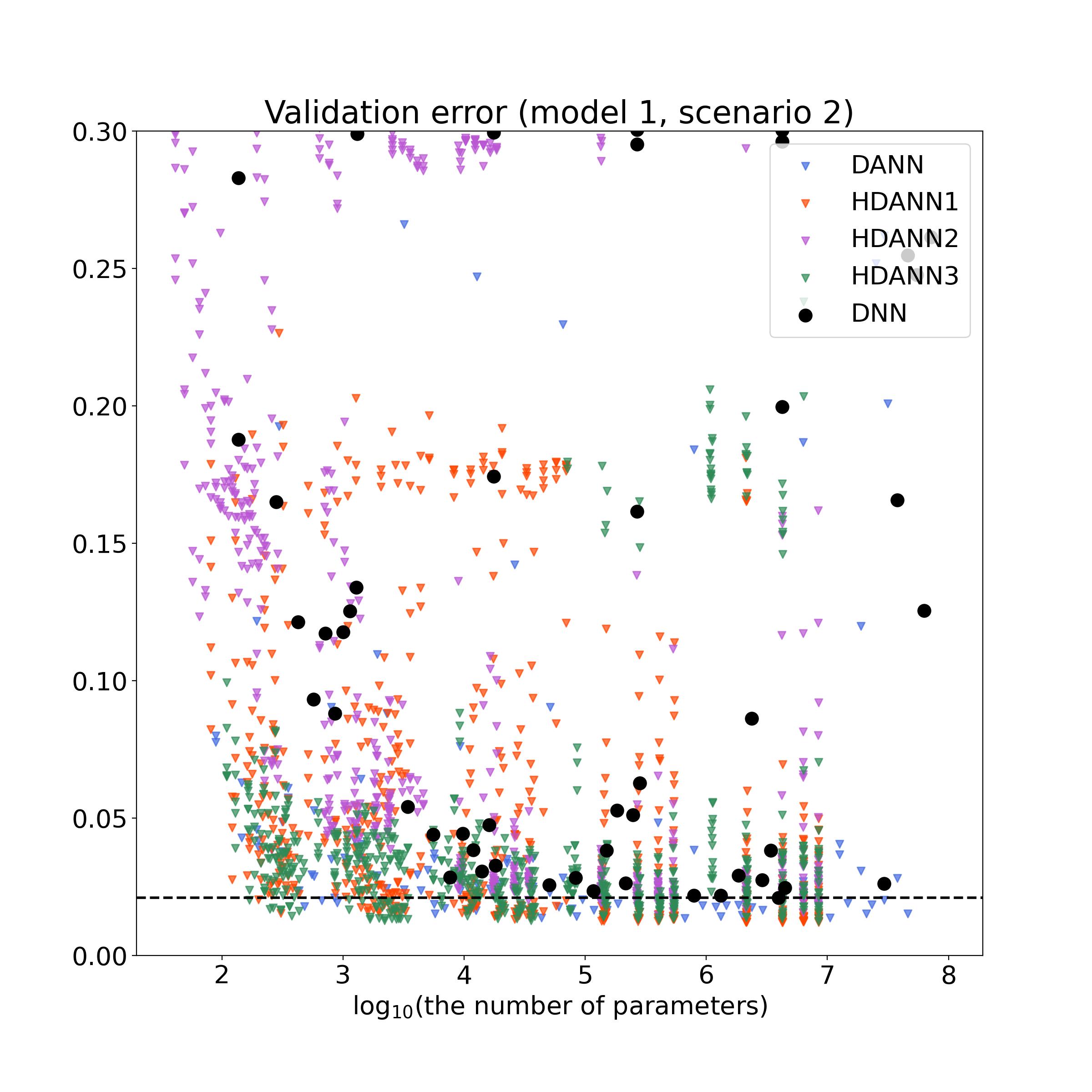
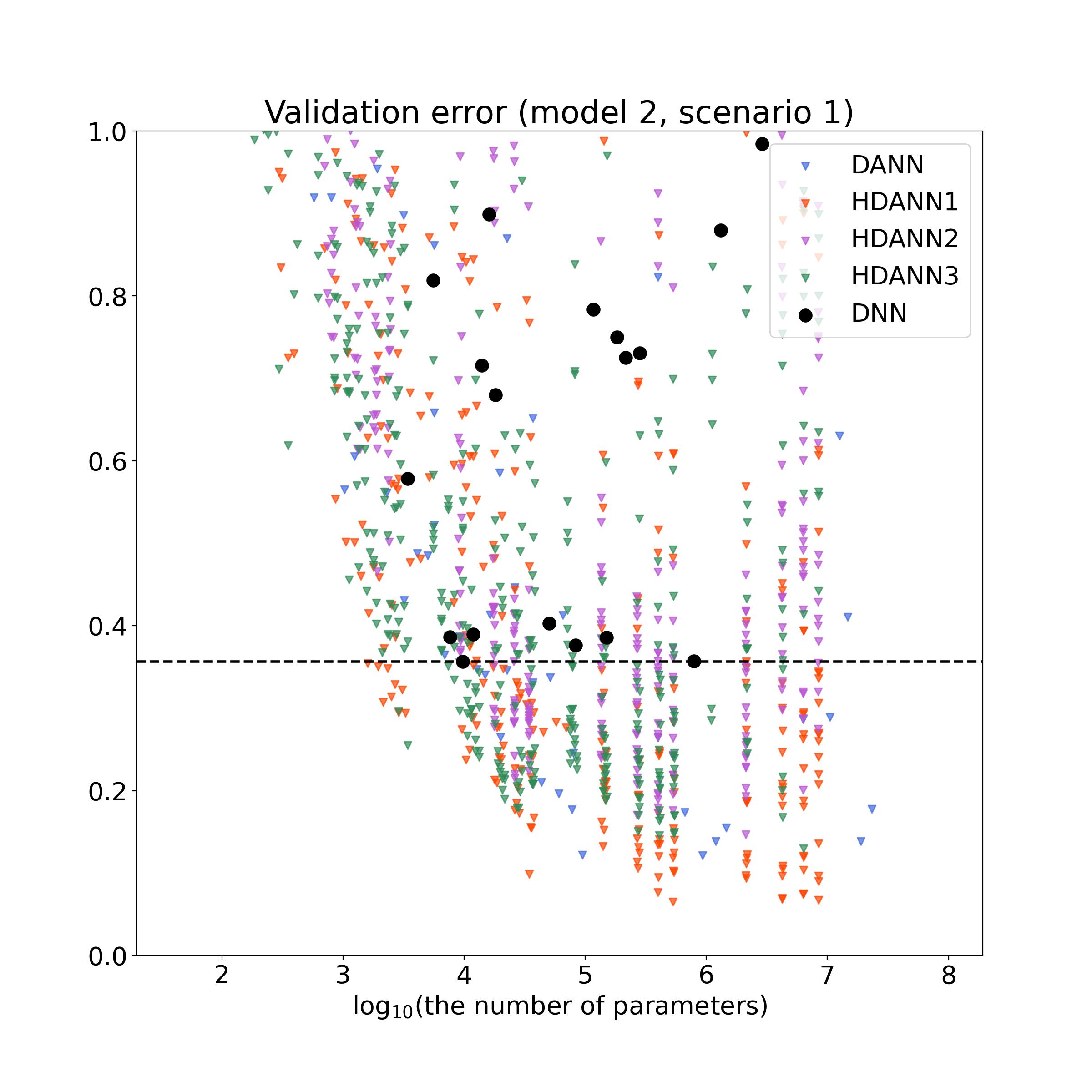
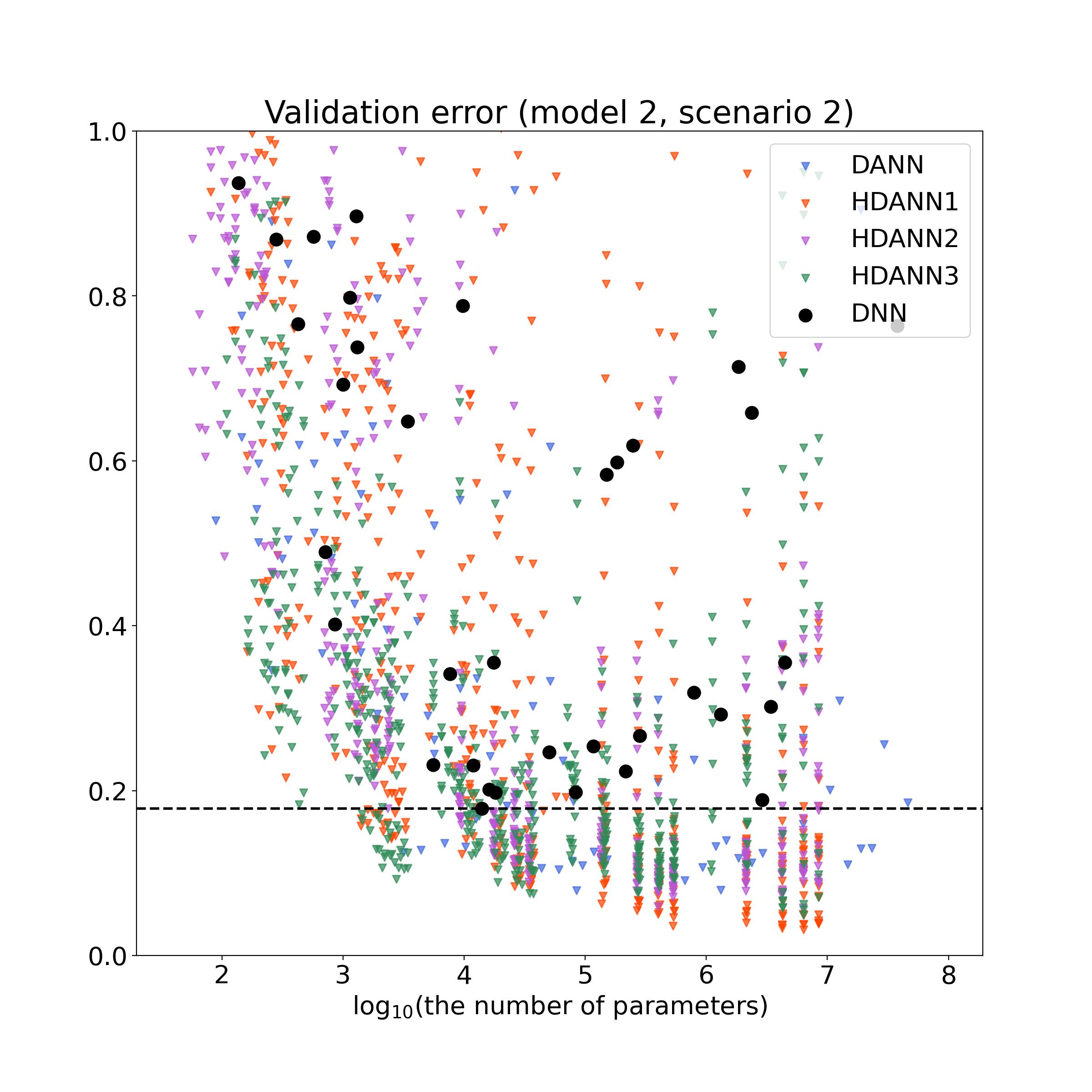
For the comparison of the numbers of parameters, we present the scatter plots of

$\displaystyle\left(\log_{10}(\text{the number of parameters}),\sum_{i\in I_{\rm validation}}(Y_{i}-\hat{Y}_{i})^{2}/500\right)$

for hyperparameter combinations giving relatively low validation errors in Figure 9. This figure tells that there always exist proposed networks that achieve lower validation errors than the DNN with much smaller numbers of parameters. This demonstrates that adopting an additive layer can significantly reduce network sizes in deep learning, which overcomes a major limitation of DNN.

Refer to caption
Refer to caption
Refer to caption
Refer to caption
Figure 9: Scatter plots of $\log_{10}(\text{the number of parameters})$ versus $\sum_{i\in I_{\rm validation}}(Y_{i}-\hat{Y}_{i})^{2}/500$ for low validation errors. The black dashed line represents the smallest validation error achieved by the DNN.

We also compared the test errors, given by $\sum_{i\in I_{\rm test}}(Y_{i}-\hat{Y}_{i})^{2}/500$, of the best-tuned DANN, HDANN1, HDANN2, HDANN3 and DNN, each selected based on the lowest validation error. The selected hyperparameters are presented in Appendix 7.3. Table 1 shows that the proposed networks outperform the DNN, with HDANN1 performing the best. Table 1 also shows that the error margins between our networks and the DNN increase as the sample size increases. Additionally, Appendix 7.3 presents that our networks have similar training times to the DNN. These results demonstrate that our networks are good alternatives to the DNN.

Table 1: Comparison of test errors for the best-tuned networks.
Model 1 Model 2
Scenario 1 Scenario 2 Scenario 1 Scenario 2
DNN 0.03219 0.02620 0.26051 0.23466
DANN 0.01699 0.01867 0.09770 0.09495
HDANN1 0.01594 0.01208 0.07388 0.02817
HDANN2 0.01961 0.01718 0.12778 0.05988
HDANN3 0.01751 0.01468 0.09299 0.06729

5 Real Data Analysis

We applied our methods to the California Housing data obtained from the sklearn Python library. This dataset consists of 9 variables across 20640 block groups. A block group is a geographical unit containing multiple houses. We used the logarithm of the median house value in each block group as $Y$. For each block group, we extracted the following variables and took them as $X_{1},\ldots,X_{8}$: Longitude of block group, Latitude of block group, Median house age, Average number of rooms, Average number of bedrooms, Population, Average number of households and Median household income.

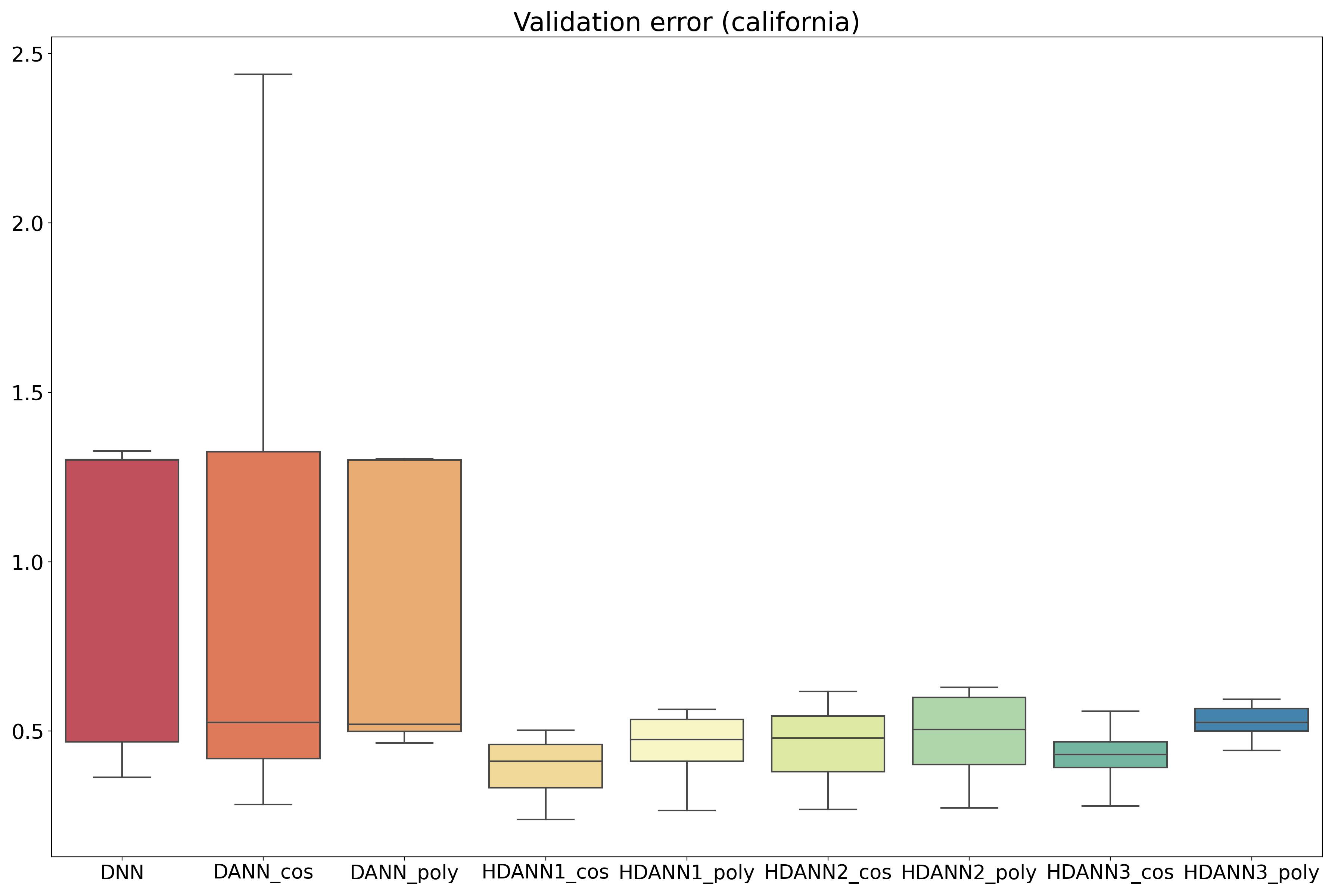
To compare the networks, we divided the observations into a training set, a validation set and a test set with proportions 60%, 20% and 20%. We scaled each $X_{j}$ by $(X_{j}-X_{j,{\rm min}})/(X_{j,{\rm max}}-X_{j,{\rm min}})$, where $X_{j,{\rm min}}$ and $X_{j,{\rm max}}$ are the the minimum and maximum values of $X_{j}$ in the training set, respectively. We trained the networks using the standardized values of $Y$ with mean and standard deviation being computed from the training set. We took the same hyperparameter combinations and optimization as in the simulation study. We then evaluated their validation errors in the original response scale. Figure 10 provides the boxplots of validation errors. It shows that the DANN generally yields comparable validation errors with the DNN, while the hybrid networks tend to have significantly lower validation errors than the DNN. In particular, the cosine basis works better than the polynomial basis for the hybrid networks.

Refer to caption
Figure 10: Boxplots of $\sum_{i\in I_{\rm validation}}(Y_{i}-\hat{Y}_{i})^{2}/|I_{\rm validation}|$ on the California Housing data. The DNN has almost the same median and Q3 values.

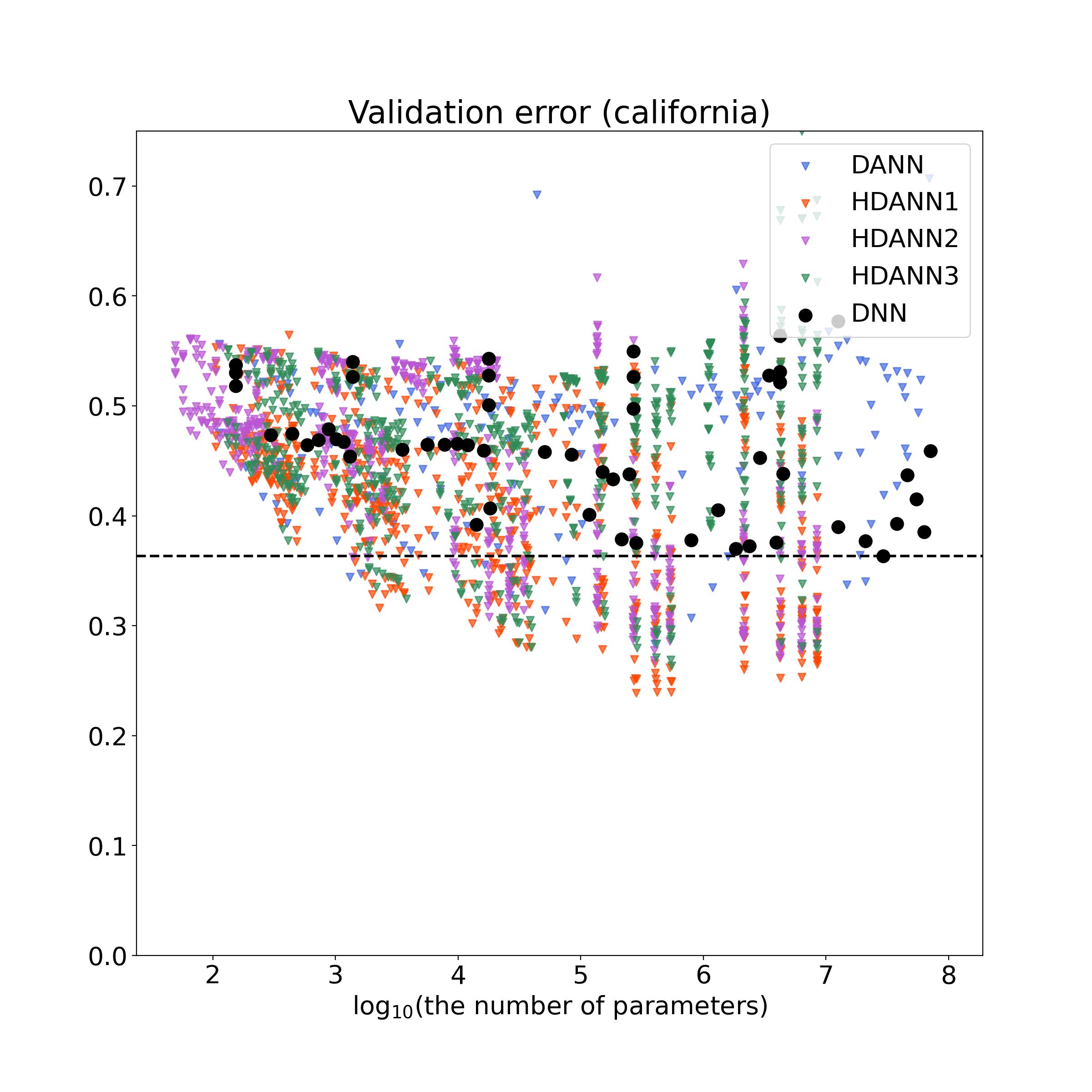
To compare the numbers of parameters, the scatter plot of

$\displaystyle\left(\log_{10}(\text{the number of parameters}),\sum_{i\in I_{\rm validation}}(Y_{i}-\hat{Y}_{i})^{2}/|I_{\rm validation}|\right)$

is obtained for hyperparameter combinations with relatively low validation errors (Figure 11). This figure illustrates that there are many proposed networks that have lower validation errors than the DNN. There also exist proposed networks that have approximately $10^{4}$-times fewer parameters but achieve the lowest validation error of DNN.

Refer to caption
Figure 11: Scatter plot of $\log_{10}(\text{the number of parameters})$ versus $\sum_{i\in I_{\rm validation}}(Y_{i}-\hat{Y}_{i})^{2}/|I_{\rm validation}|$ for low validation errors on the California Housing data. The black dashed line represents the smallest validation error achieved by the DNN.

We finally compared the best-tuned networks using test errors. The best hyperparameters and the corresponding training times are provided in Appendix 7.3. Table 2 shows that all the best-tuned proposed networks significantly outperform the best-tuned DNN, with HDANN1 performing the best. These results again confirm the superiority of our networks.

Table 2: Comparison of test errors for the best-tuned networks on the California Housing data
Test error
DNN 0.36453
DANN 0.29679
HDANN1 0.25104
HDANN2 0.26609
HDANN3 0.27910

6 Conclusion

In this works, we proposed a new nonlinear deep neural network along with hybrid variants. These networks are easy to implement due to the simple construction of activation and basis functions. These networks also achieve the universal approximation properties. We found that adding nonlinear layers enhances accuracy and can even reduce the number of parameters. The idea of this work can be applied to other topics, such as convolutional neural networks and classification problems by changing the input or output parts. We belive that our networks are promissing alternatives to the DNN.

7 Appendix

7.1 Proofs

7.1.1 Proof of Lemma 1

The desired result holds for $B_{r}(x)=x^{r}$ since the space of all polynomials on $[0,1]$ is a dense subset of the space of all continuous functions on $[0,1]$ by the Weierstrass approximation theorem.

The desired result also holds for $B_{r}(x)=\cos(r\pi x)$. To see this, define a function $\Phi:[-\pi,\pi]\rightarrow\mathbb{R}$ by $\Phi(z)=\phi(z/\pi){\rm I}(z\in[0,\pi])+\phi(-z/\pi){\rm I}(z\in[-\pi,0])$. Then, $\Phi$ is an even continuous function, and hence Fejér’s theorem (e.g., Theorem 4.32 of Pereyra and Ward (2012)) implies that a function $\sigma_{N}\Phi$ defined by

$\displaystyle\sigma_{N}\Phi(z)=\frac{1}{2\pi(N+1)}\sum_{k=0}^{N}\sum_{s=-k}^{k}\int_{-\pi}^{\pi}\Phi(t)(\cos(st)-\sqrt{-1}\sin(st))dt(\cos(sz)+\sqrt{-1}\sin(sz))$

converges uniformly to $\Phi$. Since $\sin$ is an odd function, we have $\int_{-\pi}^{\pi}\Phi(t)\sin(st)dt=0$. This with the fact that $\Phi$ is real-valued implies that

$\displaystyle\sigma_{N}\Phi(z)=\frac{1}{2\pi(N+1)}\sum_{k=0}^{N}\sum_{s=-k}^{k}\int_{-\pi}^{\pi}\Phi(t)\cos(st)dt\cos(sz)$

converges uniformly to $\Phi$. Note that $\sigma_{N}\Phi(z)$ is a linear combination of $\{\cos(sx):0\leq s\leq N\}$ since $\cos$ is an even function. Hence, for given $\epsilon>0$, there exists $N\geq 0$ and $c_{s}\in\mathbb{R}$ such that $\sup_{z\in[0,\pi]}|\Phi(z)-\sum_{s=0}^{N}c_{s}\cos(sz)|<\epsilon$. This implies that $\sup_{x\in[0,1]}|\phi(x)-\sum_{s=0}^{N}c_{s}\cos(s\pi x)|<\epsilon$.

Lastly, it is well known that the desired result holds for the Haar basis on $[0,1]$; see McLaughlin (1969), for example. $\square$

7.1.2 Proof of Theorem 1

The universal approximation theorem (Cybenko (1989)) implies that there exist constants $p\geq 1$ and $w_{k},w_{jk},a_{k}\in\mathbb{R}$ such that

$\displaystyle\sup_{\mathbf{x}\in[0,1]^{d}}\left|f(\mathbf{x})-\left(\sum_{k=1}^{p}w_{k}g\left(\sum_{j=1}^{d}w_{jk}x_{j}+a_{k}\right)\right)\right|<\frac{\epsilon}{2}.$

Note that the functions $h_{k}:x\mapsto w_{k}x$ and $h_{jk}:x_{j}\mapsto w_{jk}x_{j}+a_{k}/d$ are uniformly continuous on $[0,1]$. Hence, there exists $\delta_{k}>0$ such that

$\displaystyle\sup_{x,y\in[0,1]:|x-y|<\delta_{k}}|h_{k}(x)-h_{k}(y)|<\frac{\epsilon}{4p}.$

By the definitions of $B_{jkr}$ and $B_{k\ell}$, there exist constants $q_{k},q_{jk}\geq 1$ and $c_{k\ell},b_{k},c_{jkr},b_{jk}\in\mathbb{R}$ such that

$\displaystyle\sup_{x\in[0,1]}\left|h_{k}(x)-\left(\sum_{\ell=1}^{q_{k}}c_{k\ell}B_{k\ell}(x)+b_{k}\right)\right|$ $\displaystyle<\frac{\epsilon}{4p},$
$\displaystyle\sup_{x_{j}\in[0,1]}\left|h_{jk}(x_{j})-\left(\sum_{r=1}^{q_{jk}}c_{jkr}B_{jkr}(x_{j})+b_{jk}\right)\right|$ $\displaystyle<\frac{\delta_{k}}{dL},$

where $L>0$ is the Lipschitz constant of $g$. Define

$\displaystyle\tilde{h}_{k}(x)$ $\displaystyle=\sum_{\ell=1}^{q_{k}}c_{k\ell}B_{k\ell}(x)+b_{k},$
$\displaystyle\tilde{h}_{jk}(x_{j})$ $\displaystyle=\sum_{r=1}^{q_{jk}}c_{jkr}B_{jkr}(x_{j})+b_{jk}.$

Note that

$\displaystyle\left|g\left(\sum_{j=1}^{d}h_{jk}(x_{j})\right)-g\left(\sum_{j=1}^{d}\tilde{h}_{jk}(x_{j})\right)\right|$ $\displaystyle\leq L\left|\sum_{j=1}^{d}h_{jk}(x_{j})-\sum_{j=1}^{d}\tilde{h}_{jk}(x_{j})\right|$
$\displaystyle\leq L\sum_{j=1}^{d}|h_{jk}(x_{j})-\tilde{h}_{jk}(x_{j})|$
$\displaystyle\leq\delta_{k}.$

Then,

$\displaystyle\sup_{\mathbf{x}\in[0,1]^{d}}\left|\sum_{k=1}^{p}h_{k}\left(g\left(\sum_{j=1}^{d}h_{jk}(x_{j})\right)\right)-\sum_{k=1}^{p}\tilde{h}_{k}\left(g\left(\sum_{j=1}^{d}\tilde{h}_{jk}(x_{j})\right)\right)\right|$
$\displaystyle\leq\sup_{\mathbf{x}\in[0,1]^{d}}\sum_{k=1}^{p}\left|h_{k}\left(g\left(\sum_{j=1}^{d}h_{jk}(x_{j})\right)\right)-\tilde{h}_{k}\left(g\left(\sum_{j=1}^{d}\tilde{h}_{jk}(x_{j})\right)\right)\right|$
$\displaystyle\leq\sup_{\mathbf{x}\in[0,1]^{d}}\sum_{k=1}^{p}\left|h_{k}\left(g\left(\sum_{j=1}^{d}h_{jk}(x_{j})\right)\right)-h_{k}\left(g\left(\sum_{j=1}^{d}\tilde{h}_{jk}(x_{j})\right)\right)\right|$
$\displaystyle\quad+\sup_{\mathbf{x}\in[0,1]^{d}}\sum_{k=1}^{p}\left|h_{k}\left(g\left(\sum_{j=1}^{d}\tilde{h}_{jk}(x_{j})\right)\right)-\tilde{h}_{k}\left(g\left(\sum_{j=1}^{d}\tilde{h}_{jk}(x_{j})\right)\right)\right|$
$\displaystyle\leq\sum_{k=1}^{p}\sup_{\mathbf{x}\in[0,1]^{d}}\left|h_{k}\left(g\left(\sum_{j=1}^{d}h_{jk}(x_{j})\right)\right)-h_{k}\left(g\left(\sum_{j=1}^{d}\tilde{h}_{jk}(x_{j})\right)\right)\right|$
$\displaystyle\quad+\sum_{k=1}^{p}\sup_{\mathbf{x}\in[0,1]^{d}}\left|h_{k}\left(g\left(\sum_{j=1}^{d}\tilde{h}_{jk}(x_{j})\right)\right)-\tilde{h}_{k}\left(g\left(\sum_{j=1}^{d}\tilde{h}_{jk}(x_{j})\right)\right)\right|$
$\displaystyle\leq\sum_{k=1}^{p}\sup_{x,y\in[0,1]:|x-y|<\delta_{k}}|h_{k}(x)-h_{k}(y)|+\sum_{k=1}^{p}\sup_{x\in[0,1]}|h_{k}(x)-\tilde{h}_{k}(x)|$
$\displaystyle\leq\frac{\epsilon}{4}+\frac{\epsilon}{4}.$

Therefore,

$\displaystyle\sup_{\mathbf{x}\in[0,1]^{d}}\left|f(\mathbf{x})-\sum_{k=1}^{p}\tilde{h}_{k}\left(g\left(\sum_{j=1}^{d}\tilde{h}_{jk}(x_{j})\right)\right)\right|$
$\displaystyle\leq\sup_{\mathbf{x}\in[0,1]^{d}}\left|f(\mathbf{x})-\sum_{k=1}^{p}h_{k}\left(g\left(\sum_{j=1}^{d}h_{jk}(x_{j})\right)\right)\right|$
$\displaystyle\quad+\sup_{\mathbf{x}\in[0,1]^{d}}\left|\sum_{k=1}^{p}h_{k}\left(g\left(\sum_{j=1}^{d}h_{jk}(x_{j})\right)\right)-\sum_{k=1}^{p}\tilde{h}_{k}\left(g\left(\sum_{j=1}^{d}\tilde{h}_{jk}(x_{j})\right)\right)\right|$
$\displaystyle<\epsilon.$

7.1.3 Proof of Theorem 2

Write $\sigma_{1}=\cdots=\sigma_{L}=\sigma$. By Theorem 3.2 of Kidger and Lyons (2020), there exist $L\geq 1$, $W_{k}^{(1)}\in\mathbb{R}^{d}$, $W_{k}^{(2)},\ldots,W_{k}^{(L)}\in\mathbb{R}^{d+3}$ and $w_{k},a_{k}^{(1)},b_{k}^{(l)},b\in\mathbb{R}$ such that

$\displaystyle\sup_{\mathbf{x}\in[0,1]^{d}}\left|f(\mathbf{x})-\left(\sum_{k=1}^{d+3}w_{k}\tilde{x}_{k}^{(L)}+b\right)\right|<\frac{\epsilon}{2},$

where

$\displaystyle\tilde{x}_{k}^{(l)}$ $\displaystyle=\sigma\left({W_{k}^{(l)}}^{\mathstrut\scriptscriptstyle{\top}}\tilde{\mathbf{x}}^{(l-1)}+b_{k}^{(l)}\right)$

for $1\leq k\leq d+3$ and $2\leq l\leq L$, and

$\displaystyle\tilde{x}_{k}^{(1)}$ $\displaystyle=\sigma\left({W_{k}^{(1)}}^{\mathstrut\scriptscriptstyle{\top}}\mathbf{x}+a_{k}^{(1)}\right)$

for $1\leq k\leq d+3$. Define $M=\max\{|w_{1}|,\ldots,|w_{d+3}|\}$ and $M_{kl}=\|W_{k}^{(l)}\|_{\infty}$. Let $C>0$ denote the Lipschitz constant of $\sigma$. Define $h_{jk}:[0,1]\rightarrow\mathbb{R}$ by $h_{jk}(x_{j})=W_{kj}^{(1)}x_{j}+a_{k}^{(1)}/d$, where $W_{kj}^{(1)}$ is the $j$th entry of $W_{k}^{(1)}$. Then, $h_{jk}$ is a continuous function on $[0,1]$. By Lemma 1, there exist constants $q_{jk}\geq 1$ and $c_{jkr},b_{jk}\in\mathbb{R}$ such that

$\displaystyle\sup_{x_{j}\in[0,1]}\left|h_{jk}(x_{j})-\left(\sum_{r=1}^{q_{jk}}c_{jkr}B_{jkr}(x_{j})+b_{jk}\right)\right|<\frac{\epsilon}{2MC^{L}\left(\max_{1\leq k\leq d+3,2\leq l\leq L}M_{kl}\right)(d+3)^{L}d}.$

Define $\bar{h}_{jk}(x_{j})=\sum_{r=1}^{q_{jk}}c_{jkr}B_{jkr}(x_{j})+b_{jk}$. Then,

$\displaystyle\sup_{\mathbf{x}\in[0,1]^{d}}\left|\sigma\left({W_{k}^{(1)}}^{\mathstrut\scriptscriptstyle{\top}}\mathbf{x}+a_{k}^{(1)}\right)-\sigma\left(\sum_{j=1}^{d}\bar{h}_{jk}(x_{j})\right)\right|$
$\displaystyle\leq C\sup_{\mathbf{x}\in[0,1]^{d}}\left|\sum_{j=1}^{d}h_{jk}(x_{j})-\sum_{j=1}^{d}\bar{h}_{jk}(x_{j})\right|$
$\displaystyle\leq C\sup_{\mathbf{x}\in[0,1]^{d}}\sum_{j=1}^{d}|h_{jk}(x_{j})-\bar{h}_{jk}(x_{j})|$
$\displaystyle\leq\frac{\epsilon}{2MC^{L-1}\left(\max_{1\leq k\leq d+3,2\leq l\leq L}M_{kl}\right)(d+3)^{L}}$

Define

$\displaystyle x_{k}^{(l)}$ $\displaystyle=\sigma\left({W_{k}^{(l)}}^{\mathstrut\scriptscriptstyle{\top}}\mathbf{x}^{(l-1)}+b_{k}^{(l)}\right)$

for $1\leq k\leq d+3$ and $2\leq l\leq L$, and

$\displaystyle x_{k}^{(1)}$ $\displaystyle=\sigma\left(\sum_{j=1}^{d}\bar{h}_{jk}(x_{j})\right).$

Since

$\displaystyle\left|\sigma\left({W_{k}^{(l)}}^{\mathstrut\scriptscriptstyle{\top}}\tilde{\mathbf{x}}^{(l-1)}+b_{k}^{(l)}\right)-\sigma\left({W_{k}^{(l)}}^{\mathstrut\scriptscriptstyle{\top}}\mathbf{x}^{(l-1)}+b_{k}^{(l)}\right)\right|$ $\displaystyle\leq C|{W_{k}^{(l)}}^{\mathstrut\scriptscriptstyle{\top}}(\tilde{\mathbf{x}}^{(l-1)}-\mathbf{x}^{(l-1)})|$
$\displaystyle\leq CM_{kl}\sum_{s=1}^{d+3}|\tilde{x}^{(l-1)}_{s}-x^{(l-1)}_{s}|$

for $2\leq l\leq L$, we get

$\displaystyle\sup_{\mathbf{x}\in[0,1]^{d}}\left|\sum_{k=1}^{d+3}w_{k}\tilde{x}_{k}^{(L)}+b-\left(\sum_{k=1}^{d+3}w_{k}x_{k}^{(L)}+b\right)\right|$
$\displaystyle\leq\sup_{\mathbf{x}\in[0,1]^{d}}M\sum_{k=1}^{d+3}|\tilde{x}_{k}^{(L)}-x_{k}^{(L)}|$
$\displaystyle\leq\sup_{\mathbf{x}\in[0,1]^{d}}MC\sum_{k=1}^{d+3}M_{kL}\sum_{s=1}^{d+3}|\tilde{x}^{(L-1)}_{s}-x^{(L-1)}_{s}|$
$\displaystyle\leq\cdots$
$\displaystyle\leq\sup_{\mathbf{x}\in[0,1]^{d}}MC^{L-1}\left(\max_{1\leq k\leq d+3,2\leq l\leq L}M_{kl}\right)(d+3)^{L-1}\sum_{s=1}^{d+3}|\tilde{x}^{(1)}_{s}-x^{(1)}_{s}|$
$\displaystyle\leq\frac{\epsilon}{2}.$

Therefore,

$\displaystyle\sup_{\mathbf{x}\in[0,1]^{d}}\left|f(\mathbf{x})-\left(\sum_{k=1}^{d+3}w_{k}x_{k}^{(L)}+b\right)\right|<\epsilon.$

7.1.4 Proof of Theorem 3

Write $\sigma_{1}=\cdots=\sigma_{L-1}=g_{L}=\sigma$. By Theorem 3.2 of Kidger and Lyons (2020), there exist $L\geq 1$, $W_{k}^{(1)}\in\mathbb{R}^{d}$, $W_{k}^{(2)},\ldots,W_{k}^{(L)}\in\mathbb{R}^{d+3}$ and $w_{k},b_{k}^{(l)},a\in\mathbb{R}$ such that

$\displaystyle\sup_{\mathbf{x}\in[0,1]^{d}}\left|f(\mathbf{x})-\left(\sum_{k=1}^{d+3}w_{k}x_{k}^{(L)}+a\right)\right|<\frac{\epsilon}{2},$

where

$\displaystyle x_{k}^{(l)}$ $\displaystyle=\sigma\left({W_{k}^{(l)}}^{\mathstrut\scriptscriptstyle{\top}}\mathbf{x}^{(l-1)}+b_{k}^{(l)}\right)$

for $1\leq k\leq d+3$ and $2\leq l\leq L$, and

$\displaystyle x_{k}^{(1)}$ $\displaystyle=\sigma\left({W_{k}^{(1)}}^{\mathstrut\scriptscriptstyle{\top}}\mathbf{x}+b_{k}^{(1)}\right)$

for $1\leq k\leq d+3$. Define $h_{k}:[0,1]\rightarrow\mathbb{R}$ by $h_{k}(x_{k})=w_{k}x_{k}+a/(d+3)$. Then, $h_{k}$ is a continuous function on $[0,1]$. By Lemma 1, there exist constants $q_{k}\geq 1$ and $c_{kr},b_{k}\in\mathbb{R}$ such that

$\displaystyle\sup_{x_{k}\in[0,1]}\left|h_{k}(x_{k})-\left(\sum_{r=1}^{q_{k}}c_{kr}B_{kr}(x_{k})+b_{k}\right)\right|<\frac{\epsilon}{2(d+3)}.$

Then,

$\displaystyle\sup_{\mathbf{x}\in[0,1]^{d}}\left|\sum_{k=1}^{d+3}h_{k}(x_{k})-\sum_{k=1}^{d+3}\left(\sum_{r=1}^{q_{k}}c_{kr}B_{kr}(x_{k})+b_{k}\right)\right|<\frac{\epsilon}{2}.$

Therefore,

$\displaystyle\sup_{\mathbf{x}\in[0,1]^{d}}\left|f(\mathbf{x})-\sum_{k=1}^{d+3}\left(\sum_{r=1}^{q_{k}}c_{kr}B_{kr}(x_{k}^{(L)})+b_{k}\right)\right|<\epsilon.$

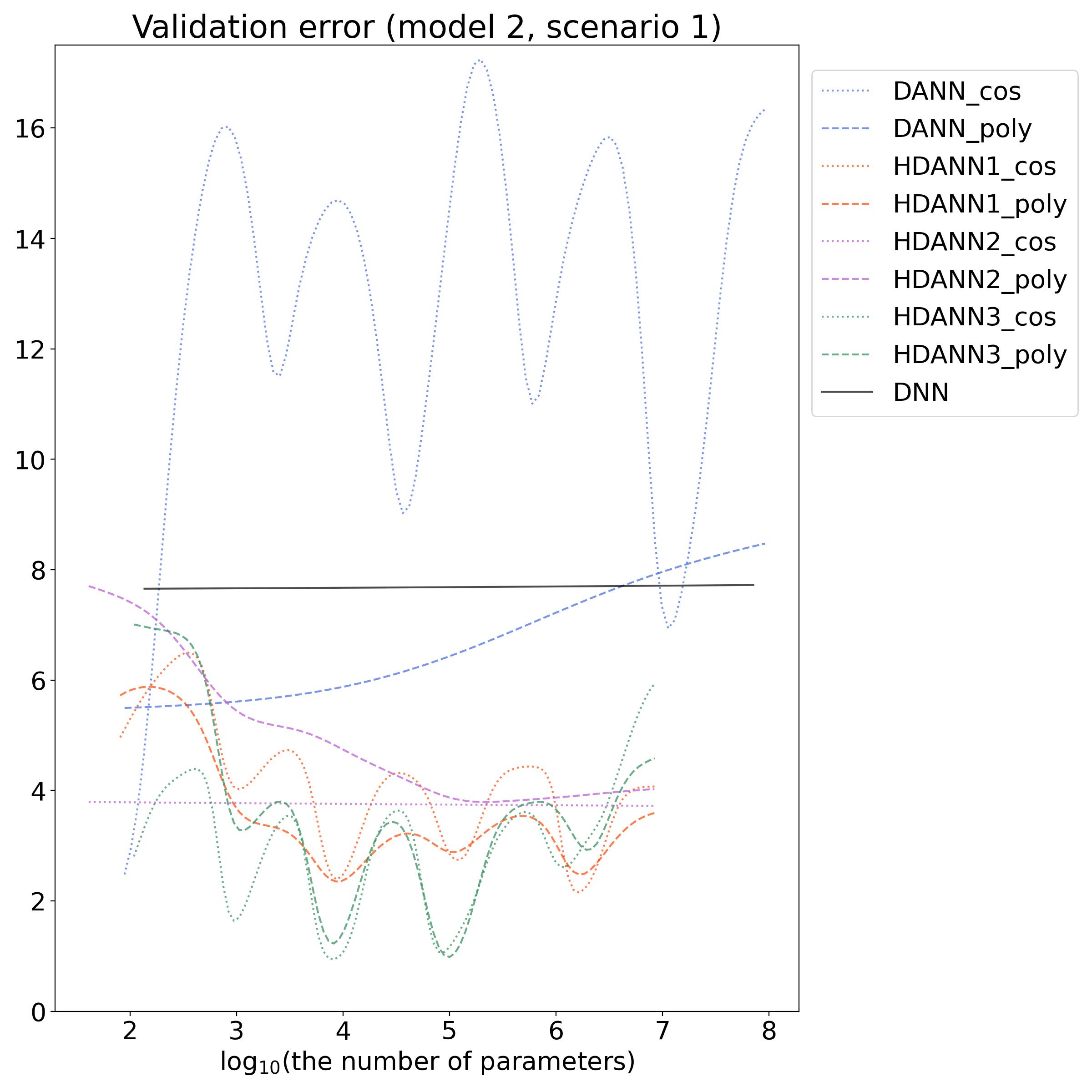
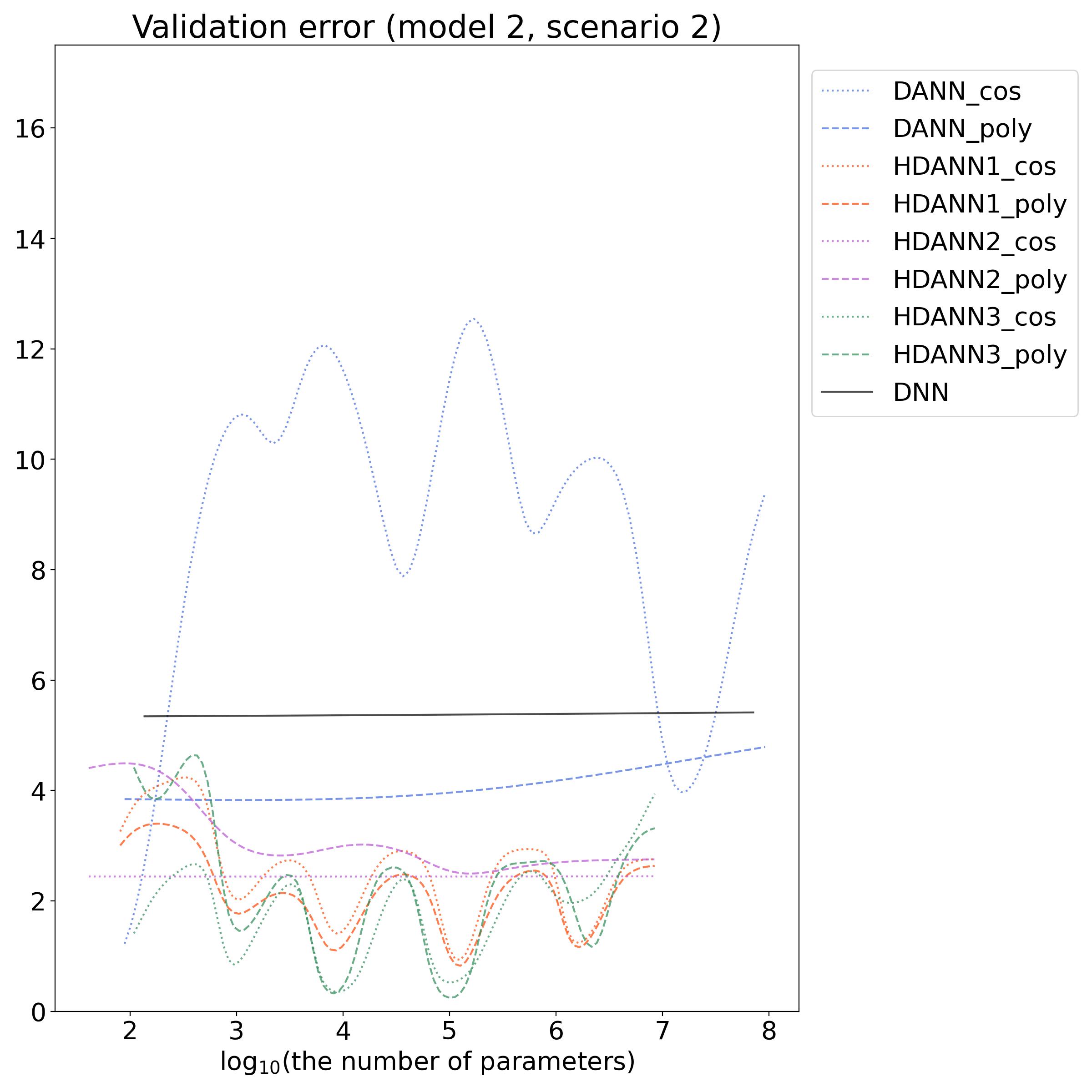
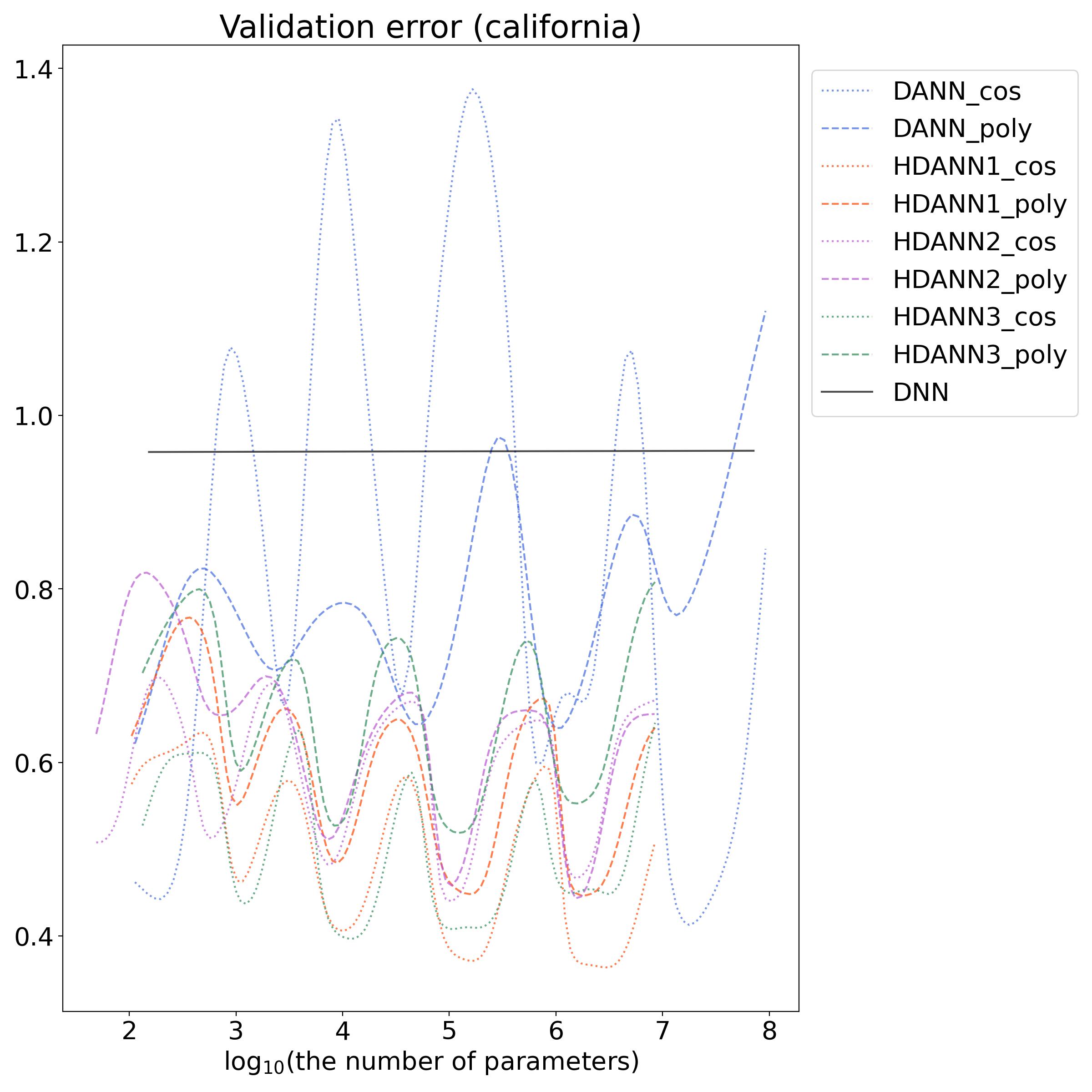
7.2 Kernel-smoothed curves of validation errors

To see the overall performance of networks, we also obtained a kernel-smoothed curve by taking

$\displaystyle\left(\log_{10}(\text{the number of parameters}),\sum_{i\in I_{\rm validation}}(Y_{i}-\hat{Y}_{i})^{2}/500\right)$

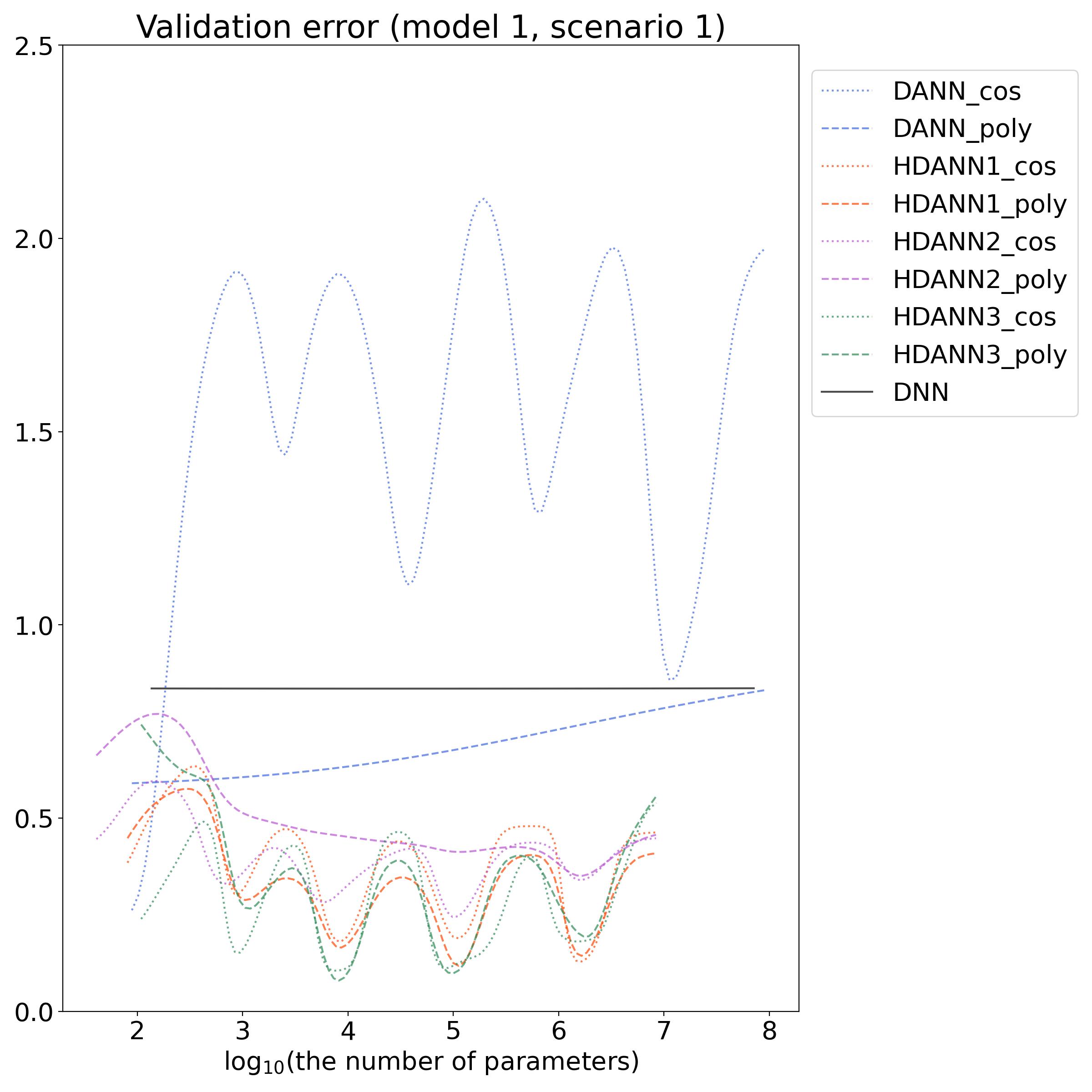
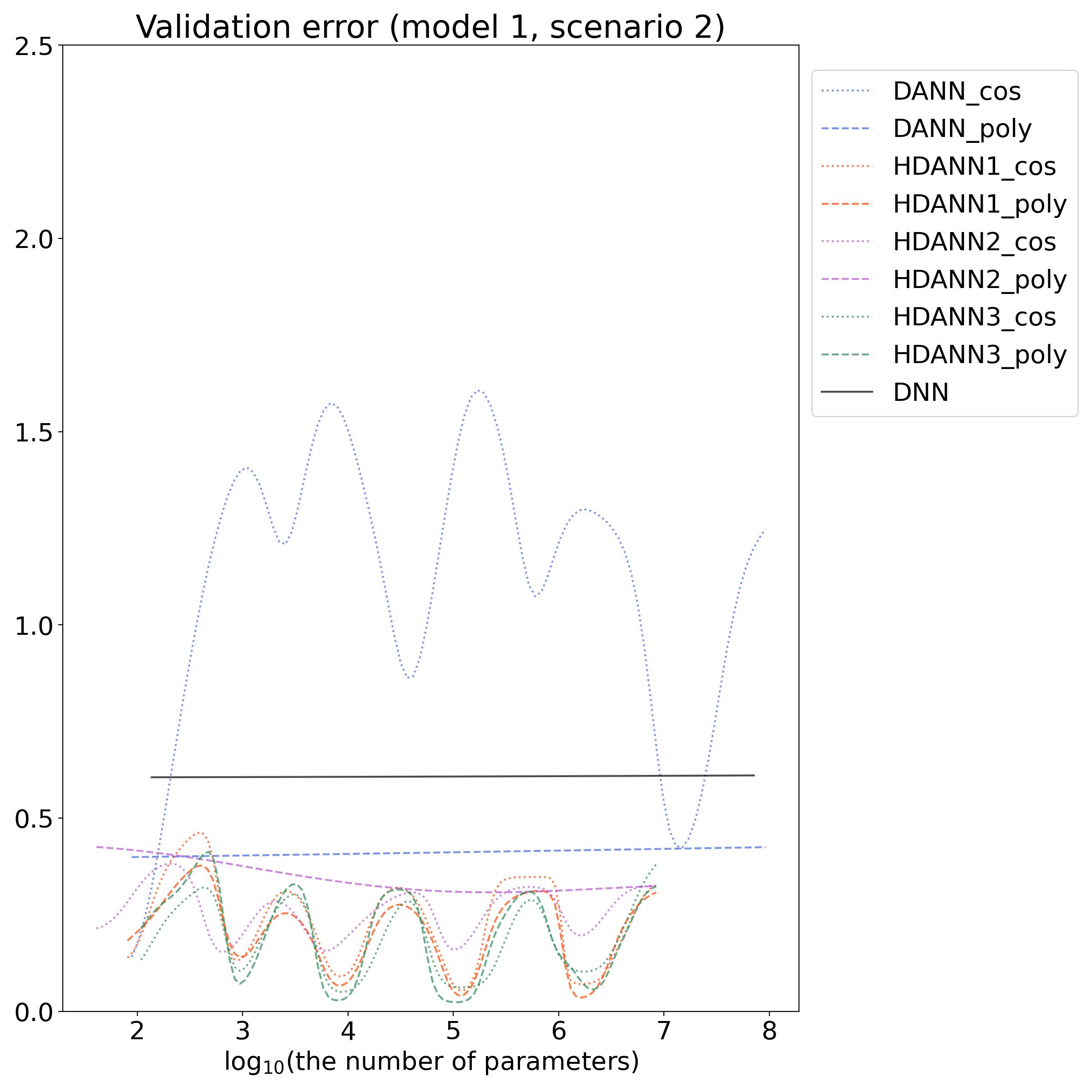
across all hyperparameter combinations as data points for each network; see Figure 12 below for the simulations and Figure 13 below for the real data application. Here, we used the Gaussian kernel and bandwidth selected by a 5-fold cross-validation. Both figures indicate that the hybrid networks generally achieve significantly lower validation errors than the DNN with fewer parameters.

Refer to caption
Refer to caption
Refer to caption
Refer to caption
Figure 12: Smoothed curves of $\log_{10}(\text{the number of parameters})$ versus $\sum_{i\in I_{\rm validation}}(Y_{i}-\hat{Y}_{i})^{2}/500$.
Refer to caption
Figure 13: Smoothed curves of $\log_{10}(\text{the number of parameters})$ versus the validation error on the California Housing data.

7.3 Top 5 results for each network

Table 3: Top 5 results for model 1 in scenario 1
Network $L$ $p$ $q$ $\sigma$ $B_{r}$ Validation Error Test Error Training Time (sec)
14 128 tanh 0.04912 0.03219 10.13
8 128 tanh 0.05148 0.03230 9.00
DNN 6 512 tanh 0.05743 0.03180 6.72
12 32 tanh 0.06210 0.04500 14.19
10 128 tanh 0.06380 0.04113 9.37
3 1024 5 poly 0.01568 0.01699 10.40
3 64 9 poly 0.01667 0.02001 7.12
DANN 3 256 11 poly 0.01690 0.01874 7.18
5 1024 7 poly 0.01710 0.01780 13.14
3 256 9 poly 0.01796 0.02009 6.31
5 1024 7 ReLU poly 0.01375 0.01594 3.84
5 1024 9 ReLU poly 0.01398 0.01596 3.87
HDANN1 7 1024 5 ReLU poly 0.01440 0.01501 4.50
9 1024 9 ReLU poly 0.01450 0.01668 5.84
3 1024 7 ReLU poly 0.01450 0.01638 2.90
7 256 9 tanh poly 0.02946 0.01961 13.14
5 256 9 tanh poly 0.03382 0.02432 11.33
HDANN2 7 256 7 tanh poly 0.03597 0.02162 10.89
5 256 7 tanh poly 0.03782 0.02628 10.57
5 256 5 tanh poly 0.03863 0.02316 10.48
9 256 11 ReLU poly 0.01648 0.01751 9.65
7 64 11 ReLU poly 0.01690 0.02037 8.66
HDANN3 5 256 7 ReLU poly 0.01725 0.02045 6.13
7 256 7 ReLU poly 0.01740 0.02079 6.35
5 256 5 ReLU poly 0.01753 0.01923 6.15
Table 4: Top 5 results for model 1 in scenario 2
Network $L$ $p$ $q$ $\sigma$ $B_{r}$ Validation Error Test Error Training Time (sec)
16 512 tanh 0.02109 0.02620 12.09
4 512 tanh 0.02187 0.02886 8.45
DNN 6 512 tanh 0.02187 0.02460 8.34
8 128 tanh 0.02358 0.02737 10.08
18 512 tanh 0.02467 0.02496 12.70
3 256 5 poly 0.01359 0.01867 8.99
3 64 5 poly 0.01371 0.02199 9.24
DANN 3 1024 5 poly 0.01379 0.01697 9.62
5 256 5 poly 0.01417 0.01878 6.77
5 64 5 poly 0.01420 0.02115 8.44
3 1024 7 ReLU poly 0.01202 0.01208 2.94
9 1024 7 ReLU poly 0.01204 0.01105 6.30
HDANN1 5 1024 7 ReLU poly 0.01211 0.01165 3.79
5 1024 9 ReLU poly 0.01213 0.01135 4.05
7 1024 5 ReLU poly 0.01220 0.01182 4.68
7 256 11 tanh poly 0.01467 0.01718 12.48
7 1024 9 tanh poly 0.01573 0.01832 12.30
HDANN2 9 256 3 tanh poly 0.01608 0.01803 11.64
3 1024 11 ReLU poly 0.01711 0.01895 8.27
9 256 9 tanh poly 0.01773 0.01920 12.73
9 1024 5 ReLU poly 0.01250 0.01468 8.10
9 64 5 tanh poly 0.01273 0.01959 10.22
HDANN3 7 16 5 tanh poly 0.01274 0.02976 15.52
7 256 5 ReLU poly 0.01284 0.01694 6.10
9 16 5 tanh poly 0.01317 0.02956 17.30
Table 5: Top 5 results for model 2 in scenario 1
Network $L$ $p$ $q$ $\sigma$ $B_{r}$ Validation Error Test Error Training Time (sec)
10 32 tanh 0.35643 0.26051 13.14
4 512 tanh 0.35724 0.25841 6.53
DNN 6 128 tanh 0.37640 0.30307 7.84
10 128 tanh 0.38573 0.33599 8.55
8 32 tanh 0.38657 0.31983 14.00
3 256 7 poly 0.12137 0.09770 7.58
3 64 11 poly 0.12170 0.12466 11.88
DANN 3 1024 9 poly 0.13835 0.10913 17.87
3 256 9 poly 0.13863 0.11562 7.74
3 256 11 poly 0.15517 0.12385 8.07
9 256 3 ReLU poly 0.06505 0.07388 5.51
9 1024 5 ReLU poly 0.06732 0.05466 6.17
HDANN1 5 1024 5 ReLU poly 0.06854 0.05299 3.97
5 1024 3 ReLU poly 0.06960 0.05787 4.07
7 1024 3 ReLU poly 0.07465 0.06317 4.77
3 1024 9 tanh poly 0.14653 0.12778 10.39
5 256 11 tanh poly 0.17055 0.14588 9.61
HDANN2 7 256 7 tanh cos 0.17248 0.09998 7.00
9 256 9 tanh cos 0.17620 0.12159 8.71
7 256 11 ReLU poly 0.17949 0.12100 7.82
7 1024 7 tanh cos 0.12975 0.09299 10.43
7 256 7 ReLU poly 0.14566 0.11879 8.33
HDANN3 9 256 7 ReLU poly 0.14774 0.11144 9.25
9 256 9 ReLU cos 0.14929 0.11932 8.97
5 256 5 ReLU poly 0.15077 0.12481 7.45
Table 6: Top 5 results for model 2 in scenario 2
Network $L$ $p$ $q$ $\sigma$ $B_{r}$ Validation Error Test Error Training Time (sec)
14 32 tanh 0.17844 0.23466 33.25
12 512 tanh 0.18859 0.24226 9.65
DNN 18 32 tanh 0.19739 0.26406 19.12
6 128 tanh 0.19806 0.24641 9.45
16 32 tanh 0.20164 0.24533 18.52
5 64 5 poly 0.07885 0.09495 16.08
5 256 5 poly 0.07961 0.07965 13.89
DANN 3 256 5 poly 0.09090 0.10638 11.08
3 64 7 poly 0.10455 0.11694 12.93
3 64 5 poly 0.10608 0.14098 12.13
7 1024 5 ReLU poly 0.03153 0.02817 5.26
5 1024 7 ReLU poly 0.03318 0.03224 4.15
HDANN1 9 256 3 ReLU poly 0.03606 0.04866 5.66
5 1024 3 ReLU poly 0.03630 0.03108 4.07
7 1024 9 ReLU poly 0.03747 0.03945 5.11
7 1024 3 ReLU poly 0.05802 0.05988 7.84
7 256 5 ReLU poly 0.05982 0.06848 7.71
HDANN2 9 256 9 tanh poly 0.07126 0.07858 12.34
5 1024 3 ReLU poly 0.07386 0.08772 6.34
5 1024 7 ReLU poly 0.07488 0.07438 7.42
7 1024 11 ReLU cos 0.04894 0.06729 12.37
7 1024 9 tanh cos 0.05595 0.07085 12.33
HDANN3 5 1024 9 tanh cos 0.05781 0.06659 11.10
5 1024 11 tanh cos 0.05861 0.06277 12.09
7 1024 11 tanh cos 0.06245 0.07909 13.55
Table 7: Top 5 results on the California Housing data
Network $L$ $p$ $q$ $\sigma$ $B_{r}$ Validation Error Test Error Training Time (sec)
8 2048 tanh 0.36354 0.36452 29.77
8 512 tanh 0.37023 0.36686 17.86
DNN 10 512 tanh 0.37234 0.37399 20.28
18 128 tanh 0.37548 0.37957 34.45
16 512 tanh 0.37565 0.37385 30.38
3 256 3 cos 0.28369 0.29679 24.64
5 256 3 cos 0.30702 0.31787 17.99
DANN 5 64 3 cos 0.31432 0.31953 23.33
3 64 3 cos 0.32797 0.32584 28.35
7 256 3 cos 0.33481 0.34992 17.20
5 256 9 tanh cos 0.23888 0.25104 31.65
7 256 11 tanh cos 0.23966 0.25363 35.98
HDANN1 9 256 9 tanh cos 0.23968 0.25718 35.54
7 256 9 tanh cos 0.24727 0.26066 29.99
9 256 11 tanh cos 0.24906 0.25813 24.60
7 256 7 ReLU cos 0.26842 0.26609 29.61
5 1024 11 ReLU cos 0.27161 0.27309 21.64
HDANN2 5 1024 5 ReLU poly 0.27318 0.27249 26.69
7 256 3 ReLU cos 0.27788 0.27524 27.44
7 1024 7 ReLU poly 0.27826 0.27896 27.26
9 256 11 tanh cos 0.26357 0.2791 42.70
9 256 7 tanh cos 0.26913 0.27683 52.30
HDANN3 7 256 7 tanh cos 0.27107 0.28388 47.06
9 1024 9 ReLU cos 0.27909 0.29561 27.21
5 256 11 tanh cos 0.27965 0.29149 26.30

References

  • Bauer and Kohler (2019) Bauer, B. and Kohler, M. (2019). On deep learning as a remedy for the curse of dimensionality in nonparametric regression. Annals of Statistics, 47, 2261–2285.
  • Bilodeau (1992) Bilodeau, M. (1992). Fourier smoother and additive models. Canadian Journal of Statistics, 20, 241–351.
  • Cybenko (1989) Cybenko, G. (1989). Approximation by superpositions of a sigmoidal function. Mathematics of Control, Signals, and Systems, 2, 303–314.
  • Fakhoury et al. (2022) Fakhoury, D., Fakhoury, E. and Speleers, H. (2022). ExSpliNet: An interpretable and expressive spline-based neural network. Neural Networks, 152, 332–346.
  • Glorot and Bengio (2010) Glorot, X. and Bengio, Y. (2010). Understanding the difficulty of training deep feedforward neural networks. AISTATS, 9, 249–256.
  • Haar (1910) Haar, A. (1910). Zur Theorie der orthogonalen Funktionensysteme. Mathematische Annalen, 69, 331–371.
  • Horowitz and Mammen (2007) Horowitz, J. L. and Mammen, E. (2007). Rate-optimal estimation for a general class of nonparametric regression models with unknown link functions. Annals of Statistics, 35, 2589–2619.
  • Jeon and Park (2020) Jeon, J. M. and Park, B. U. (2020). Additive regression with Hilbertian responses. Annals of Statistics, 48, 2671–2697.
  • Jeon et al. (2022) Jeon, J. M., Lee, Y. K., Mammen, E. and Park, B. U. (2022). Locally polynomial Hilbertian additive regression. Bernoulli, 28, 2034–2066.
  • Kidger and Lyons (2020) Kidger, P. and Lyons, T. (2020). Universal Approximation with Deep Narrow Networks. Proceedings of Machine Learning Research, 125, 1–22.
  • Kingma and Ba (2017) Kingma, D. P. and Ba, J, M. (2017). Adam: A Method for Stochastic Optimization. arXiv:1412.6980v9.
  • Kohler and Langer (2021) Kohler, M. and Langer, S. (2021). On the rate of convergence of fully connected deep neural network regression estimates. Annals of Statistics, 49, 2231–2249.
  • Kolmogorov (1957) Kolmogorov, A. N. (1957). On the representation of continuous functions of many variables by superposition of continuous functions of one variable and addition. Doklady Akademii Nauk SSSR, 114, 953–956.
  • LeCun et al. (2015) LeCun, Y., Bengio, Y. and Hinton, G. (2015). Deep learning. Nature, 521, 436–444.
  • Linton and Nielsen (1995) Linton, O. and Nielsen, J. P. (1995). A kernel method of estimating structured nonparametric regression based on marginal integration. Biometrika, 82, 93–101.
  • Liu et al. (2024) Liu, Z., Wang, Y., Vaidya, S., Ruehle, F., Halverson, J., Soljačić, M., Hou, T. Y. and Tegmark, M. (2024). KAN: Kolmogorov-Arnold Networks. arXiv:2404.19756v4.
  • Mammen et al. (1999) Mammen, E., Linton, O. B. and Nielsen, J. P. (1999). The existence and asymptotic properties of a backfitting projection algorithm under weak conditions. Annals of Statistics, 27, 1443–1490.
  • McLaughlin (1969) McLaughlin, J. R. (1969). Haar Series. Transactions of the American Mathematical Society, 137, 153–176.
  • Meier et al. (2009) Meier, L., van de Geer, S. and Bühlmann, P. (2009). High-dimensional additive modeling. Annals of Statistics, 37, 3779–3821.
  • Opsomer and Ruppert (1997) Opsomer, J. D. and Ruppert, D. (1997). Fitting a bivariate additive model by local polynomial regression. Annals of Statistics, 25, 186–211.
  • Pereyra and Ward (2012) Pereyra, M. C. and Ward, L. A. (2012). Harmonic Analysis: From Fourier to Wavelets. American Mathematical Society.
  • Sardy and Ma (2024) Sardy, S. and Ma, X. (2024). Sparse additive models in high dimensions with wavelets. Scandinavian Journal of Statistics, 51, 89–-108.
  • Schmidt-Hieber (2020) Schmidt-Hieber, J. (2020). Nonparametric regression using deep neural networks with ReLU activation function. Annals of Statistics, 48, 1875–1897.
  • Schmidhuber (2015) Schmidhuber, J. (2015). Deep learning in neural networks: An overview. Neural Networks, 61, 85–117.