Coarsening and universality on a growing surface

Abstract

We introduce a model in which particles belonging to two species proliferate with volume exclusion on an expanding surface. If the surface expands uniformly, we show that the domains formed by the two species present a critical behavior. We compute the critical exponents characterizing the decay of interfaces and the size distribution of domains using a mean-field theory. These mean-field exponents agree very accurately with those fitted in numerical simulations, suggesting that the theory is exact.

Introduction

Many biological systems are composed of dense proliferating cells [1]. Due to proliferation, these systems often grow [2, 3], or alternatively, occupy a tissue undergoing its own expansion [4, 5]. From a theoretical perspective, the way a domain grows can profoundly affect dynamical processes taking place on it. For example, the formation of Turing patterns can be controlled by domain growth [6, 7, 8]. The case of uniform stretch, besides being the simplest, has revealed peculiar properties, akin to those of critical systems, in morphogen gradient dynamics [9] and in disordered packing [10]. More generally, domain growth can generate long-term temporal correlations in dynamics. Examples include genetic drift at the growing perimeter of a bacteria colonies and tumors [11, 12, 13], and Kardar-Parisi-Zhang dynamics in liquid crystals [14]. Complex behavior due to expansion emerges in discrete (lattice) models as well, where surface growth can control competition outcomes by affecting spatial correlations [15, 16].

In this work, we present a model in which two neutral species proliferate on an expanding surface with volume exclusion. We call the model the “growing voter model”, in analogy with the traditional voter model in non-equilibrium statistical physics. We demonstrate that coarsening in the growing voter model becomes critical for uniform growth. We calculate the critical exponents associated with the decay of interfaces and the cluster size distribution by a mean-field approach. Simulation results are consistent with the mean-field exponents to a high degree of accuracy, suggesting that the mean-field solution is exact.

Growing voter model

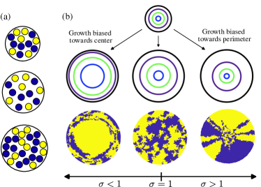
Figure 1: Dynamics of the growing voter model. (a) As the surface grows, space is created and yellow (+) and blue (-) cells proliferate into it. (b) Contour lines associated with the displacement field $\lambda(\mu,\sigma,t)$. For $\sigma<1$, this results in one cell type ultimately dominating the surface. When growth is uniform, $\sigma=1$, neither cell type dominates and a seemingly critical behavior emerges. For $\sigma>1$, the dynamics leads to the formation of sectors.

Our model describes a cell population consisting of two types of cells, that we denote by $+$ and $-$, placed on a growing circular surface of radius $R(t)$. We call $N_{+}(t)$ and $N_{-}(t)$ the numbers of $+$ and $-$ cells at time $t$, respectively. The total number of cells is $N(t)=N_{+}(t)+N_{-}(t)$. Cells proliferate at a constant rate, identical for the two types. When a cell proliferates, it creates a new cell of the same type a distance $2c$ from its own center, where $c$ is a cell’s radius, at an angle chosen uniformly at random, see Fig. 1a. If the newly created cell overlaps with an existing cell, the proliferation event is aborted. The surface radially expands at a speed given by the displacement field $\lambda(r,\sigma,t)=(r/R(t))^{\sigma}$, where $r$ is the distance from the center of the surface. The parameter $\sigma>0$ tunes the stretching protocol. In particular, for $\sigma<1$ or $\sigma>1$, the surface grows more rapidly close to the center or boundary, respectively (see Fig. 1b). In the limiting case $\sigma=1$, the stretching rate is uniform. We term this model the “growing voter model” as its basic ingredients (reproduction and competition between two statistically identical species) resemble those of the voter model.

Simulations show that the growing voter model generates different patterns depending on how the surface grows, see Fig. 1b. In particular, for $\sigma<1$, one of the two types fixates at the center of the surface, while competition between the two types occurs at the perimeter. For $\sigma>1$, the two types occupy radial sectors, reminiscent of competing bacterial strains on agar plates [11]. In the case of uniform stretch ($\sigma=1$), the two species form domains without an apparent characteristic scale, suggesting a sort of critical behavior.

To characterize the behavior for $\sigma=1$, we study the density of interfaces $\rho(t)$, defined as the number of Voronoi neighbor pairs that are of different colors divided by the total number of pairs. Simulations show that the density of interfaces decays as

$$\rho\sim N(t)^{-\alpha}\,,$$ (1)

with $\alpha\approx 0.305$, see Fig. 2.

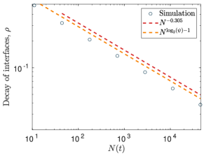
Figure 2: Decay of interfaces for uniform surface growth, see Fig. 1 b. An interface is defined as a pair of Voronoi neighbors that are of different colors. The fit of simulation data yields $N^{-0.305}$ with 95% confidence intervals (-0.306, -0.304), red dashed line. The dashed magenta line represents $N^{\log_{2}(\psi)-1}$, see Eq. (6).

I Lattice model

To find an expression for the decay of the interface density, we study a discrete time, lattice version of the growing voter model. Each site of a two-dimensional square contains a $\pm 1$ cell. At each step, the sides of the square lattice are doubled in length, and new empty sites are added to the lattice as illustrated in Fig. 3. We call $n_{0}\times n_{0}$ initial system size, so that at the $k^{th}$ step the system size is equal to $2^{k}n_{0}\times 2^{k}n_{0}$. The preexisting cells determine the type of the newly inserted cells in the following manner: if a new empty site has two preexisting neighbors, one of these two neighbors is chosen uniformly at random to proliferate into this empty site. If a new site has no occupied neighbors, its color is uniformly and randomly chosen from one of the four preexisting diagonal sites.

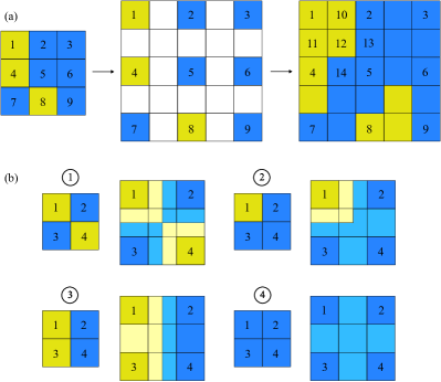
Figure 3: The two-dimensional lattice model. (a) At each time step the length of the domain in both the horizontal and vertical directions is doubled. The cell type of empty new sites are filled by selecting from their neighbors uniformly at random. For instance, the new site 10 is filled by selecting from 1 or 2. The new site 11 is filled by selecting from 1 or 4. The new site 12 is filled by selecting from 1, 2, 4 or 5. (b) Doubling of elementary cells in the mean-field theory. The sites of a lighter shade indicate the new sites created by a growth event.

In the lattice model, we define an interface as two neighbors who share an edge having different spin values. The density of interfaces is the number of interfaces divided by the total number of neighbors ($n_{0}^{2}2^{2k}$ at iteration $k$, assuming periodic boundary conditions). We derive the decay rate of the density of interfaces in the lattice model by a mean-field assumption. We focus on a $2\times 2$ elementary cell. Assuming rotational and $Z_{2}$ symmetry, there are four possible types of elementary cells:

$$\raisebox{0.5pt}{\raisebox{-.9pt} {1}⃝}=\begin{pmatrix}+1&-1\\ -1&+1\end{pmatrix},\raisebox{0.5pt}{\raisebox{-.9pt} {2}⃝}=\begin{pmatrix}+1&-1\\ +1&-1\end{pmatrix},$$ (2)

$$\raisebox{0.5pt}{\raisebox{-.9pt} {3}⃝}=\begin{pmatrix}+1&+1\\ +1&-1\end{pmatrix},\raisebox{0.5pt}{\raisebox{-.9pt} {4}⃝}=\begin{pmatrix}+1&+1\\ +1&+1\end{pmatrix}.$$

We calculate the proportions at which each of these configurations generate other ones at each step. For instance, configuration \raisebox{-.9pt} {1}⃝ generates the configurations $\underline{p}=\left(\raisebox{0.5pt}{\raisebox{-.9pt} {1}⃝},\raisebox{0.5pt}{\raisebox{-.9pt} {2}⃝},\raisebox{0.5pt}{\raisebox{-.9pt} {3}⃝},\raisebox{0.5pt}{\raisebox{-.9pt} {4}⃝}\right)$ in proportions $(1/8,1/4,1/2,1/8)$. We call $\underline{p}(k)$ the vector encoding the frequency of the four different elementary cell types in the system. The evolution of this vector is governed by a Markov chain

$$p(k+1)=\hat{M}p(k)\,,$$ (3)

where

$$\hat{M}=\begin{pmatrix}\frac{1}{8}&0&\frac{1}{64}&0\\ \frac{1}{4}&\frac{1}{4}&\frac{5}{32}&0\\ \frac{1}{2}&\frac{1}{2}&\frac{7}{16}&0\\ \frac{1}{8}&\frac{1}{4}&\frac{25}{64}&1\end{pmatrix}.$$ (4)

The leading eigenvalue of the matrix $\hat{M}$ is equal to 1, with an associated right eigenvector $(0,0,0,1)$. This eigenvector represents the absorbing state in which only one of the two spins is present in the system. The second eigenvalue of $\hat{M}$ is equal to $(1+\sqrt{5})/4$. which implies that the interfaces asymptotically decay as

$$\rho(2^{k}n_{0}\times 2^{k}n_{0}) \sim\left(\frac{1+\psi}{4}\right)^{k}\,,$$ (5)

where $\psi=(1+\sqrt{5})/2$ is the golden ratio. To return to continuous time, we let $t\sim 2^{k}$, so that $k\sim\log_{2}(t)\sim\frac{1}{2}\log_{2}(N(t))$, and so we obtain

$$\rho\sim N(t)^{-\alpha}\quad\mbox{with}\quad\alpha=1-\log_{2}(\psi).$$ (6)

This scaling is plotted in Fig. 2. We simulated the lattice model up to $k=17$ (approximately $17\cdot 10^{9}$ lattice sites). The relative discrepancy between the simulation and Eq. (6) is on the order of $10^{-7}$. This lattice model also appears to exhibit the same exponent as our off-lattice model. For example, the relative error between the off-lattice model and the analytical formula at a system size of $10^{5}$ cells (comparable to $k=8$ in the lattice model) is equal to $10^{-4}$. In Appendix A, we present further statistical comparison between the discrete model and the analytical solution.

I.1 Comparison with the voter model

It is interesting to compare the scaling of interfaces between the growing voter model and the traditional voter model, see Table 1. In one dimension, interfaces are conserved in the growing voter model and thus their density decays as $t^{-1}$ due to dilution. In contrast, in the one-dimensional voter model they present a diffusive decay $t^{-1/2}$. In two dimensions, the scaling derived in this section contrasts with the logarithmic scaling found in the conventional voter model [17].

Dimension	Voter model	Growing voter model
1D	$t^{-\frac{1}{2}}$	$t^{-1}$
2D	$(\mathrm{ln}t)^{-1}$	$\frac{1}{2}t^{2(\log_{2}(\psi)-1)}$

Table 1: Comparison between the voter model and the growing voter model.

We also analyze a well-mixed version of our model (see Appendix B). This well-mixed version is equivalent to the Pólya urn model; in contrast, in the well-mixed limit, the voter model becomes the Moran model of population genetics (see Appendix B). We also derived a stochastic partial differential equation (PDE) governing the dynamics of the growing voter model in the rescaled frame of reference (Appendix C). In one dimension, this has dynamics equivalent to that of the voter model, but with a nonlinear time transformation in which time presents a critical slowdown. This equivalence, however, does not hold in two dimensions (Appendix C).

I.2 Fractal dimension of interfaces

We now use the rate of decay of interfaces to derive the behavior of other observables. We begin by deriving the fractal dimension of the interfaces.

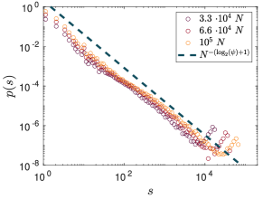
Figure 4: Scaling of clusters in the growing voter model with uniform stretch. A cluster is defined as a Voronoi-connected component of cells of the same type. Each simulation replicate was initialized with 20 cells of randomly chosen type. The total number of simulation replicates for each system size is 1000.

The fractal dimension $D$ is defined by

$$Q=\epsilon^{-D},$$ (7)

where $Q$ is the number of interfaces (usually referred to as the ‘number of measurement units’ in the fractal literature) and $\epsilon$ is the rescaling factor. In our case, the rescaling factor is analogous to growth: every time a growth event occurs all distances within the system are halved, which is equivalent to dividing $\epsilon$ by two. Given this, we write Eq. (7) for our system as

$$(4^{k}n^{2}_{0})^{1-\alpha}\sim\left(\frac{1}{2^{k}}\right)^{-D}\,.$$ (8)

In the limit of $k\rightarrow\infty$ we obtain

$$D=2(1-\alpha)\,.$$ (9)

Substituting the value of $\alpha$ given by Eq. (6), we obtain $D=\log_{2}(1+\psi)=1.388483...$, which is twice the fractal dimension of the asymmetric Cantor set ($\log_{2}(\psi)$).

I.3 Scaling and number of clusters

We define as a cluster a connected set of Voronoi neighbors having the same spin value. The distribution of cluster sizes for large $N$ also appears to decays as a power law at the critical point:

$$p(s)=\frac{n(s)}{\tilde{n}}\sim s^{-\beta}\,,$$ (10)

where $n(s)$ is the number of clusters of size $s$ and $\tilde{n}$ is the total number of clusters, see Fig. 4.

To compute the exponent $\beta$, we assume that clusters are seeded proportionally to the number of interfaces, and once present grow deterministically and proportionally to the domain size. This assumption implies

$$s(N;N_{0})=\left(\frac{N}{N_{0}}\right)\,,$$ (11)

where $s(N;N_{0})$ is the size of a cluster at system size $N$ that was seeded at system size $N_{0}$.

We now assume that clusters are seeded proportionally to the number of interfaces in the system. This assumption implies $d\tilde{n}/dN\ \sim N^{-\alpha}$ (see Eq. (1)), and therefore

$$\tilde{n}\sim N^{1-\alpha}\,.$$ (12)

We now rewrite Eq. (11) in terms of numbers of clusters, expressing only the dependence on $\tilde{n}_{0}$:

$$s(\tilde{n}_{0})\sim\tilde{n}_{0}^{-1/(1-\alpha)}\,.$$ (13)

Picking a random cluster amounts to sampling $\tilde{n}_{0}$ in a uniform manner, so that $p(s)\propto d\tilde{n}_{0}/ds$. Using Eq. (10) and Eq. (13) we therefore obtain

$$\beta=2-\alpha.$$ (14)

This prediction is in excellent agreement with simulation results, see Fig. 4.

II Discussion

We have introduced a novel phase transition in which the control parameter is how the surface is grown. We have identified uniform stretch as a critical point, and characterized it by the decay of interfaces. We have also characterized the fractal dimension of the interfaces and the scaling of cluster size.

To analyze this system we turned to an lattice-based model, that we solved by a mean-field approach. The close agreement between this solution and simulations suggests that the solution is exact. A reason for this could be that propagation of information in the voter dynamics is diffusive, whereas the ballistic (i.e., linear in time) nature of growth causes lattice sites to behave independently of their neighbors. This argument would also explain why the observed scaling of cluster sizes can be accounted for by assuming that each cluster evolves in a statistically independent way.

Appendix A Decay of interfaces: statistical analysis

In Fig. 5 we plot the exponent of the decay of the interfaces from simulations compared against the analytical formula. In the case of a 2-by-2 initial lattice grown 17 generations (20000 replicates) the error in the calculation of the slope with the analytic formula is $3.2\times 10^{-7}$. For any initial domain whose size is $2^{k}\times 2^{k}$ the formula quickly converges. For other sizes of initial system the convergence is slower.

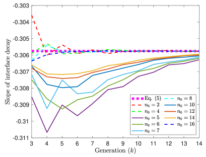
Figure 5: The numerically calculated slope of interface decay in the lattice model compared to the slope of interface decay for Eq. (5), for different initial lattice sizes.

Appendix B Mean-field analysis

We now analyze our growing voter in the well-mixed regime. To do so we envisage a cell population containing both $N_{+}$ and $N_{-}$ cells, so that $N=N_{+}+N_{-}$. We denote by $f$ the density of $N_{+}$ cells,

$$f=\frac{N_{+}}{N}\,.$$ (15)

In the limit of large $N$ we can write

$$N(t)=\kappa N_{0}(1+(P_{g}t/N_{0})),$$

where $\kappa$ is the number of cells per unit size and $P_{g}$ is the growth rate of the system. We further define

$$\frac{dN(t)}{dt}=P_{g}\kappa=\Gamma.$$

Returning to the discrete setting, in a proliferation event, $\frac{N_{+}+1}{N+1}$ with probability $f$, and $\frac{N_{+}}{N+1}$ with probability $1-f$. In the first instance, the change in $f$ is

$$\Delta f=\frac{N_{+}+1}{N+1}-\frac{N_{+}}{N}=\frac{N-N_{+}}{N(N+1)}=\frac{(1-f)}{N+1},$$ (16)

while in the second

$$\Delta f=\frac{N_{+}}{N+1}-\frac{N_{+}}{N}=\frac{-N_{+}}{N(N+1)}=\frac{-f}{N+1}.$$ (17)

The expected change in $f$ is

$$\langle\Delta f\rangle=f((1-f)/(N+1))+(1-f)(-f/(N+1))=0,$$ (18)

and the second moment is

$$\langle\Delta f^{2}\rangle =f((1-f)/(N+1))^{2}+(1-f)(-f/(N+1))^{2}$$

$$=f(1-f)/(N+1)^{2}\sim f(1-f)/N^{2}.$$ (19)

These moments correspond to the Langevin equation

$$\frac{\mathrm{d}f}{\mathrm{d}t}=\sqrt{\frac{\Gamma(1-f)f}{N^{2}}}\gamma(t),$$ (20)

$$\langle\gamma(t_{1})\gamma(t_{2})\rangle=\delta(t_{1}-t_{2}),$$ (21)

where $\gamma(t)$ is a white, zero mean Gaussian noise and $\delta(t)$ is the Dirac delta-function. The Fokker-Planck equation (FPE) corresponding to Eq. (20) is

$$\frac{\partial p(x,t)}{\partial t}=\frac{\partial^{2}}{\partial x^{2}}\Bigg{[}\frac{\Gamma x(1-x)}{2N^{2}}p(x,t)\Bigg{]}.$$ (22)

As the number of cells increases linearly, this becomes

$$\frac{\partial p(x,t)}{\partial t}=\frac{\Gamma}{2N^{2}}\frac{\partial^{2}}{\partial x^{2}}[x(1-x)p(x,t)].$$ (23)

We now simplify Eq. (23) by employing the following change of variables [18]

$$d\tau=\frac{\Gamma dt}{2N(t)^{2}},$$ (24)

whereby

$$\tau =\int_{0}^{t}\frac{\Gamma}{2N(t)^{2}}dt=\int_{0}^{t}\frac{P_{g}\kappa}{2N(t)^{2}}dt$$

$$=\frac{1}{2}\left(\frac{1}{N_{0}}-\frac{1}{N_{0}(1+P_{g}t)}\right),$$ (25)

and so obtain the FPE

$$\frac{\partial p(x,\tau)}{\partial\tau}=\frac{1}{2}\frac{\partial^{2}}{\partial x^{2}}\left[x(1-x)p\right].$$ (26)

From the definition of $\tau$ it can be seen that asymptotically the dynamics of the model ’freezes’, and the initial number of balls in the urn determines the asymptotic bound of $\tau$, a distinctive feature of Pólya urn dynamics. This freezing dynamics is characteristic of growing systems [11, 14], and also reminiscent of glassy systems [19]. The solution to Eq. (26), in this instance taken from [20] and with the initial condition $\delta(u_{0})$, is

$$P(u,t)=u_{0}(1-u_{0})\sum_{m=0}^{\infty}c_{m}F_{m}(1-2u_{0})F_{m}(1-2x)e^{-\frac{1}{2}(m+1)(m+2)t},$$ (27)

where $F_{m}(x)$ are the associated Jacobi polynomials $P_{m}^{(1,1)}(z)$ and $c_{m}=[(2m+3)(m+2)]/(m+1)$. Numerical simulations closely agree with this solution, see Fig. 6. Asymptotically, the distribution given in Eq. (27) approaches the $\beta$-distribution,

$$\beta(f;l,d)\propto f^{(l-1)}(1-f)^{(d-1)}\,,$$ (28)

which is the limiting distribution of the Pólya urn process [21]. In Fig. 6 we also compare the $\beta$-distribution with densities computed from simulations.

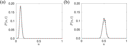
Figure 6: The evolution of the mean-field density of the two-species model. Ensemble average from simulation (black dashed), Eq. (27) (cyan dashed), and $\beta$-distribution (red) for $t=200$. In (a) $N_{+}(0)=20$ and $N_{-}(0)=180$, in (b) $N_{+}(0)=100$ and $N_{-}(0)=100$.

B.1 Extension to voter model dynamics

Here we extend our mean-field model to include a non-zero death rate. We define

$$\nu=\frac{P_{d}N^{a}}{P_{d}N^{a}+P_{g}},$$

and

$$\omega=\frac{P_{g}}{P_{d}N^{a}+P_{g}},$$

where $P_{d}$ is the death rate of both yellow and blue cells, and $P_{g}$ is the growth rate (implicitly the proliferation rate) of the system. In the mean-field regime we obtain

$$\langle\Delta f\rangle =-\nu\frac{(1-f)f}{(N-1)}+\nu\frac{(1-f)f}{(N-1)}$$

$$-\omega\frac{(1-f)f}{(N+1)}+\omega\frac{(1-f)f}{(N+1)}=0,$$ (29)

and

$$\langle\Delta f^{2}\rangle=\nu\frac{f(1-f)}{(N-1)^{2}}+\omega\frac{f(1-f)}{(N+1)^{2}}\sim(\nu+\omega)\frac{f(1-f)}{N^{2}},$$

where we have assumed that the probability of a color flipping is proportional to the product of its density with the density of the other color, as in the Moran model. The resulting Langevin equation is

$$\frac{\mathrm{d}f}{\mathrm{d}t}=\sqrt{\frac{(P_{d}N^{a}\nu+P_{g}\kappa\omega)(1-f)f}{N^{2}}}\xi(t).$$ (30)

The corresponding FPE is

$$\frac{\partial p}{\partial t}=\frac{(P_{d}N^{a}\nu+P_{g}\kappa\omega)}{2N^{2}}\frac{\partial^{2}}{\partial x^{2}}[x(1-x)p].$$ (31)

Asymptotically we have

$$\frac{\partial p}{\partial t}=\frac{P_{d}}{N^{2-a}}\frac{\partial^{2}}{\partial x^{2}}[x(1-x)p],$$ (32)

in which $\tau$ diverges when $a\geq 1$ given the definition of $\tau$, Eq. B. For $a<1$ some fraction of domains do not fixate, while for $a\geq 1$ all domains eventually fixate. Fixation time at $a=1$ is logarithmic, and fixation time is a function of the equation parameters. This recapitulates results found in Ref. [18].

Appendix C Spatially-extended case

We now consider the spatially-extended case. We consider a growing line of length $L(t)$ at time $t$, with coordinate $x\in[0,L(t)]$. We also introduce the rescaled coordinate $\xi=x/L(t)$, see [6].

C.1 One-dimensional stretch

We consider a growing ring, and describe it as a collection of connected ‘urns’ labeled by an index $i$. The length of the ring grows at rate $\Gamma$, in proportion $p(i)$ for each urn. Urns remain of constant size in the rescaled frame of reference, where nonuniform growth induces an effective flux between the urns. The boundaries $[0,x_{1},...,x_{i},...,x_{L-1}]$ of the urns evolve as

$$x_{i}(t)=x_{i}(0)\left(1+\frac{P_{g}}{L(t)}t\right).$$ (33)

We now focus on urn $i$. When this urn has grown enough to accommodate another cell, we have $N_{+}\rightarrow N_{+}+1$ and $N_{-}\rightarrow N_{-}$, and $N_{+}\rightarrow N_{+}$ and $N_{-}\rightarrow N_{-}+1$. In this instance $f_{i}^{\prime}=\frac{N_{+}+1}{N+1}$ with probability

$$p(i)\left(f_{i}\left(1-\frac{1}{N}\right)+\frac{1}{2N}\left(f_{i-1}+f_{i+1}\right)\right),$$ (34)

and $f_{i}^{\prime}=\frac{N_{l}}{N+1}$ with probability

$$p(i)\left((1-f_{i})\left(1-\frac{1}{N}\right)+\frac{1}{2N}\left((1-f_{i-1})+(1-f_{i+1})\right)\right).$$ (35)

Here, $p(i)$ indicates the probability that the proliferation event occurred in urn $i$. Therefore,

$$\langle\Delta f_{i}\rangle =\frac{p(i)}{(N+1)}\Bigg{(}(1-f)\Bigg{[}f_{i}\left(1-\frac{1}{N}\right)+\frac{1}{2N}\left(f_{i-1}+f_{i+1}\right)\Bigg{]}-f\Bigg{[}(1-f_{i})\left(1-\frac{1}{N}\right)+\frac{1}{2N}\left((1-f_{i-1})+(1-f_{i+1})\right)\Bigg{]}\Bigg{)}$$ (36)

and so

$$\langle\Delta f_{i}\rangle =\frac{p(i)}{(N+1)(2N)}\left(f_{i-1}-2f_{i}+f_{i+1}\right)$$

$$\sim\frac{p(i)}{2N^{2}}\left(f_{i-1}-2f_{i}+f_{i+1}\right),$$ (37)

and

$$\langle\Delta f_{i}^{2}\rangle\sim(p(i)f_{i}(1-f_{i}))/N^{2},$$ (38)

where we ignored $O(N^{-3})$ terms. In the case of uniform stretch $p(i)$ is the same for all urns, i.e. uniformly distributed, and so our stochastic PDE is

$$\frac{\partial f(\xi,t)}{\partial t} =\frac{\Gamma}{2N^{2}}\left(\frac{\partial^{2}f}{\partial\xi^{2}}\right)+\sqrt{\frac{\Gamma\delta\xi f(1-f)}{N^{2}}}\gamma(\xi,t),$$ (39)

where $\Gamma=P_{g}\kappa$. This equation can be rewritten as

$$\frac{\partial f(\xi,\tau)}{\partial\tau} =\Gamma\left(\frac{\partial^{2}f}{\partial\xi^{2}}\right)+\sqrt{\Gamma\delta\xi f(1-f)}\gamma(\xi,\tau),$$ (40)

which is the field theory describing the voter model in one dimension [22], albeit with freezing dynamics. At the end of this section, we demonstrate that the uniformly growing torus cannot be mapped into the voter model field theory in two dimensions by a time rescaling as for the one dimensional case.

C.2 Mean-field characterization of position of interfaces on a growing ring

On a ring containing $N$ cells there are $N$ boundaries between sites. The probability that a proliferation event involves a specific boundary is equal to $1/N$. Therefore, $\langle\Delta x\rangle$ and $\langle\Delta x^{2}\rangle$ are expressed by

$$\langle\Delta x\rangle=\bar{c}_{d}\frac{1}{2N}-\bar{c}_{d}\frac{1}{2N}=0,$$ (41)

where $\bar{c}_{d}=c_{d}/2$, and

$$\langle\Delta x^{2}\rangle=\bar{c}_{d}^{2}\frac{1}{2N}+\bar{c}_{d}^{2}\frac{1}{2N}=\frac{c_{d}^{2}}{N},$$ (42)

which means

$$\frac{\mathrm{d}x}{\mathrm{d}t}=\sqrt{\frac{P_{g}\kappa\bar{c}_{d}^{2}}{N}}\xi(t).$$ (43)

The corresponding FPE is

$$\frac{\partial p}{\partial t}=\frac{P_{g}\kappa\bar{c}_{d}^{2}}{2N}\frac{\partial^{2}p}{\partial x^{2}},$$ (44)

and so

$$\frac{\partial p}{\partial\tau}=\bar{c}_{d}^{2}\frac{\partial^{2}p}{\partial x^{2}},$$ (45)

where $\tau$ is

$$\tau =\int_{0}^{t}\frac{P_{g}\kappa}{2N_{0}(1+\frac{P_{g}t}{L})}$$

$$=\frac{1}{2}\log\left(N_{0}\left(1+\frac{P_{g}t}{L_{0}}\right)\right)-\frac{1}{2}\log(N_{0})$$

$$=\frac{1}{2}\log\left(1+\frac{P_{g}t}{L_{0}}\right),$$ (46)

and so in this instance the initial number of cells does not matter. The solution of Eq. (45) is

$$P(x,\tau)=\frac{e^{\frac{-x^{2}}{4\bar{c}_{d}^{2}\tau}}}{\sqrt{4\pi\bar{c}_{d}^{2}\tau}},$$ (47)

where $p(x,\tau)=P(x,\tau)dx$, and the root mean squared displacement is $\sqrt{2\bar{c}_{d}^{2}\tau}$. In Fig. 7 it can be seen that ensemble averages from simulations and solution Eq. (47) show close agreement.

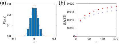
Figure 7: (a) Comparison between simulation ensemble averages (blue bars) and Eq. (47) (red line) of the evolution of interfaces on the ring. (b) Comparison of the root mean squared displacement calculated from simulations (blue dots) and $\sqrt{2\bar{c}_{d}^{2}\tau}$ (filled red dots).

C.3 Uniform stretch in two dimensions

In the case of a uniformly growing torus we have

$$\langle\Delta f_{i,j}\rangle =\frac{p(i,j)}{(N_{i}N_{j}+1)}\Bigg{(}(1-f_{i,j})\Bigg{[}f_{i,j}\left(1-\frac{(N_{i}-2)}{2(N_{i}N_{j})}-\frac{(N_{j}-2)}{2(N_{i}N_{j})}-\frac{2}{(N_{i}N_{j})}\right)$$

$$+f_{i-1,j}\left(\frac{(N_{j}-2)}{4(N_{i}N_{j})}+\frac{1}{4(N_{i}N_{j})}\right)+f_{i+1,j}\left(\frac{(N_{j}-2)}{4(N_{i}N_{j})}+\frac{1}{4(N_{i}N_{j})}\right)$$

$$+f_{i,j-1}\left(\frac{(N_{i}-2)}{4(N_{i}N_{j})}+\frac{1}{4(N_{i}N_{j})}\right)+f_{i,j+1}\left(\frac{(N_{i}-2)}{4(N_{i}N_{j})}+\frac{1}{4(N_{i}N_{j})}\right)\Bigg{]}$$

$$-f_{i,j}\Bigg{[}(1-f_{i,j})\left(1-\frac{(N_{i}-2)}{2(N_{i}N_{j})}-\frac{(N_{j}-2)}{2(N_{i}N_{j})}-\frac{2}{(N_{i}N_{j})}\right)$$

$$+(1-f_{i-1,j})\left(\frac{(N_{j}-2)}{4(N_{i}N_{j})}+\frac{1}{4(N_{i}N_{j})}\right)+(1-f_{i+1,j})\left(\frac{(N_{j}-2)}{4(N_{i}N_{j})}+\frac{1}{4(N_{i}N_{j})}\right)$$

$$+(1-f_{i,j-1})\left(\frac{(N_{i}-2)}{4(N_{i}N_{j})}+\frac{1}{4(N_{i}N_{j})}\right)+(1-f_{i,j+1})\left(\frac{(N_{i}-2)}{4(N_{i}N_{j})}+\frac{1}{4(N_{i}N_{j})}\right)\Bigg{]}\Bigg{)},$$ (48)

where $N_{i}$ and $N_{j}$ are the expected number of cells along the horizontal width of the compartment and the vertical width of the compartment, respectively. From Eq. (48) we obtain

$$\langle\Delta f_{i,j}\rangle =\frac{p(i,j)(N_{j}-2)}{(N_{i}N_{j}+1)(4N_{i}N_{j})}\left(f_{i-1,j}-2f_{i,j}+f_{i+1,j}\right)+\frac{p(i,j)(N_{i}-2)}{(N_{i}N_{j}+1)(4N_{i}N_{j})}\left(f_{i,j-1}-2f_{i,j}+f_{i,j+1}\right)$$

$$\sim\frac{p(i,j)}{4N_{i}^{2}N_{j}}\left(f_{i-1,j}-2f_{i,j}+f_{i+1,j}\right)+\frac{p(i,j)}{4N_{i}N_{j}^{2}}\left(f_{i,j-1}-2f_{i,j}+f_{i,j+1}\right),$$ (49)

where we have discarded $O((N_{i}N_{j})^{-2})$ terms, and

$$\langle\Delta f_{i,j}^{2}\rangle\sim(p(i,j)f_{i,j}(1-f_{i,j}))/(N_{i}N_{j})^{2},$$ (50)

where we have kept $O((N_{i}N_{j})^{-2})$ terms. As before $p(i,j)$ is a constant, and so our stochastic PDE is

$$\frac{\partial f(\xi_{x},\xi_{y},t)}{\partial t} =\frac{\Gamma}{4N_{x}^{2}N_{y}}\left(\frac{\partial^{2}f}{\partial\xi_{x}^{2}}\right)+\frac{\Gamma}{4N_{x}N_{y}^{2}}\left(\frac{\partial^{2}f}{\partial\xi_{y}^{2}}\right)+\sqrt{\frac{\Gamma\delta\xi_{x}\delta\xi_{y}f(1-f)}{(N_{x}N_{y})^{2}}}\gamma(\xi_{x},\xi_{y},t).$$ (51)

Equation (51) cannot be transformed into the field theory describing the two-dimensional voter model in the same way as Eq. (39). In fact, asymptotically the noise term vanishes and we are left with a ‘freezing’ diffusion equation.

C.4 Noise at the boundary

We briefly discuss how to numerically integrate our solutions via a split-step integration [Dornic2005, 23, 24, 25]. When $\theta<f<1-\theta$ we employ the Milstein method (order 1). When $f<\theta$ or $f>1-\theta$ we solve the diffusion and noise terms separately. Using the approximation $f\approx f-f^{2}$ when $f$ is small we rewrite the local Langevin as

$$\frac{\mathrm{d}f}{\mathrm{d}t}=\sqrt{\frac{\Gamma p(\xi_{x},\xi_{y})f}{N^{2}}},$$ (52)

which is associated with the FPE

$$\frac{\partial P(f,t)}{\partial t}=\frac{\Gamma p(\xi_{x},\xi_{y})}{N^{2}}\frac{\partial}{\partial^{2}f}\left[fP(f,t)\right].$$ (53)

Implementing the same transformation of variables as before, Eq. (B), we obtain

$$\frac{\partial P(f,\tau)}{\partial\tau}=\Gamma p(\xi_{x},\xi_{y})\frac{\partial^{2}}{\partial^{2}f}\left[fP(f,\tau)\right],$$ (54)

for which the solution is known [23, 26]. This distribution can be efficiently sampled [Dornic2005, 25]. Equation (54) further demonstrates that the distribution describing the noise term asymptotically freezes as the systems grows.

References

- Hallatschek et al. [2023] O. Hallatschek, S. S. Datta, K. Drescher, J. Dunkel, J. Elgeti, B. Waclaw, and N. S. Wingreen, Proliferating active matter, Nature Reviews Physics 5, 407 (2023).
- Dell’Arciprete et al. [2018] D. Dell’Arciprete, M. L. Blow, A. T. Brown, F. D. Farrell, J. S. Lintuvuori, A. F. McVey, D. Marenduzzo, and W. C. Poon, A growing bacterial colony in two dimensions as an active nematic, Nature communications 9, 4190 (2018).
- Tjhung and Berthier [2020] E. Tjhung and L. Berthier, Analogies between growing dense active matter and soft driven glasses, Phys. Rev. Research 2, 043334 (2020).
- Mort et al. [2016] R. L. Mort, R. J. H. Ross, K. J. Hainey, O. Harrison, M. A. Keighren, G. Landini, R. E. Baker, K. J. Painter, I. J. Jackson, and C. A. Yates, Reconciling diverse mammalian pigmentation patterns with a fundamental mathematical model, Nature Communications 7 (2016).
- McLennan et al. [2015] R. McLennan, L. J. Schumacher, J. A. Morrison, J. M. Teddy, D. A. Ridenour, A. C. Box, C. L. Semerad, H. Li, W. McDowell, D. Kay, et al., Neural crest migration is driven by a few trailblazer cells with a unique molecular signature narrowly confined to the invasive front, Development 142, 2014 (2015).
- Crampin et al. [1999] E. J. Crampin, E. A. Gaffney, and P. K. Maini, Reaction and diffusion on growing domains: Scenarios for robust pattern formation, Bulletin of Mathematical Biology 61, 1093 (1999).
- Crampin et al. [2002] E. J. Crampin, W. W. Hackborn, and P. K. Maini, Pattern formation in reaction-diffusion models with nonuniform domain growth, Bulletin of mathematical biology 64, 747 (2002).
- Krause et al. [2019] A. L. Krause, M. A. Ellis, and R. A. Van Gorder, Influence of curvature, growth, and anisotropy on the evolution of turing patterns on growing manifolds, Bulletin of mathematical biology 81, 759 (2019).
- Aguilar-Hidalgo et al. [2018] D. Aguilar-Hidalgo, S. Werner, O. Wartlick, M. González-Gaitán, B. M. Friedrich, and F. Jülicher, Critical point in self-organized tissue growth, Physical review letters 120, 198102 (2018).
- Ross et al. [2024] R. J. Ross, G. D. Masucci, C. Y. Lin, T. L. Iglesias, S. Reiter, and S. Pigolotti, Hyperdisordered cell packing on a growing surface, arXiv preprint arXiv:2409.15712 (2024).
- Hallatschek et al. [2007] O. Hallatschek, P. Hersen, S. Ramanathan, and D. R. Nelson, Genetic drift at expanding frontiers promotes gene segregation, Proceedings of the National Academy of Sciences 104, 19926 (2007).
- Lavrentovich and Nelson [2014] M. O. Lavrentovich and D. R. Nelson, Asymmetric mutualism in two-and three-dimensional range expansions, Physical review letters 112, 138102 (2014).
- Lavrentovich and Nelson [2015] M. O. Lavrentovich and D. R. Nelson, Survival probabilities at spherical frontiers, Theoretical population biology 102, 26 (2015).
- Takeuchi [2018] K. A. Takeuchi, An appetizer to modern developments on the Kardar–Parisi–Zhang universality class, Physica A: Statistical Mechanics and its Applications 504, 77 (2018).
- Ross et al. [2016] R. J. H. Ross, R. E. Baker, and C. Yates, How domain growth is implemented determines the long term behaviour of a cell population through its effect on spatial correlations., Physical Review E 94, 012408 (2016).
- Ross et al. [2017] R. J. H. Ross, C. A. Yates, and R. E. Baker, Variable species densities are induced by volume exclusion interactions upon domain growth, Physical Review E 95, 032416 (2017).
- Dornic et al. [2001] I. Dornic, H. Chaté, J. Chave, and H. Hinrichsen, Critical coarsening without surface tension: The universality class of the voter model, Physical Review Letters 87, 045701 (2001).
- Morris and Rogers [2014] R. G. Morris and T. Rogers, Growth-induced breaking and unbreaking of ergodicity in fully-connected spin systems, Journal of Physics A: Mathematical and Theoretical 47, 342003 (2014).
- Debenedetti and Stillinger [2001] P. G. Debenedetti and F. H. Stillinger, Supercooled liquids and the glass transition, Nature 410, 259 (2001).
- Baxter et al. [2007] G. Baxter, R. Blythe, and A. McKane, Exact solution of the multi-allelic diffusion model, Mathematical Biosciences 209, 124 (2007).
- Eggenberger and Pólya [1923] F. Eggenberger and G. Pólya, Über die statistik verketteter vorgänge, ZAMM-Journal of Applied Mathematics and Mechanics/Zeitschrift für Angewandte Mathematik und Mechanik 3, 279 (1923).
- Dickman and Tretyakov [1995] R. Dickman and A. Y. Tretyakov, Hyperscaling in the Domany-Kinzel cellular automaton, Phys. Rev. E 52, 3218 (1995).
- Pechenik and Levine [1999] L. Pechenik and H. Levine, Interfacial velocity corrections due to multiplicative noise, Phys. Rev. E 59, 3893 (1999).
- Villa Martín et al. [2019] P. Villa Martín, M. A. Muñoz, and S. Pigolotti, Bet-hedging strategies in expanding populations, PLOS Computational Biology 15, 1 (2019).
- Weissmann et al. [2018] H. Weissmann, N. M. Shnerb, and D. A. Kessler, Simulation of spatial systems with demographic noise, Phys. Rev. E 98, 022131 (2018).
- Feller [1951] W. Feller, Two singular diffusion problems, Annals of Mathematics 54, 173 (1951).
Acknowledgements
We thank Leticia Cugliandolo and Kazumasa Takeuchi for useful discussions.