STAR-RIS Enabled ISAC Systems: Joint Rate Splitting and Beamforming Optimization

Yuan Liu,  Ruichen Zhang,  Ruihong Jiang,  Yongdong Zhu,  Huimin  Hu, 
Qiang Ni, ,  Zesong Fei, ,  Dusit Niyato
Yuan Liu and Yongdong Zhu are with the Research Center for Space Computing System, Zhejiang Laboratory, Hangzhou, 311100, China (e-mail: liuyuan@bjtu.edu.cn, zhuyongdong@hotmail.com). Ruichen Zhang and Dusit Niyato are with the College of Computing and Data Science, Nanyang Technological University, Singapore 639798 (email: ruichen.zhang@ntu.edu.sg, dniyato@ntu.edu.sg). Ruihong Jiang is with the State Key Laboratory of Networking and Switching Technology, Beijing University of Posts and Telecommunications, Beijing 100876, China (e-mail: rhjiang@bupt.edu.cn). Huimin Hu is with the School of Communications and Information Engineering and the School of Artificial Intelligence, Xi’an University of Posts and Telecommunications, Xi’an 710121, China (e-mail:huiminhu@xupt.edu.cn). Qiang Ni is with the School of Computing and Communications, Lancaster University, Lancaster, LA1 4WA, United Kingdom (e-mail: q.ni@lancaster.ac.uk). Zesong Fei is with the School of Information and Electronics, Beijing Institute of Technology, Beijing 100081, China (E-mail: feizesong@bit.edu.cn).
Abstract

This paper delves into an integrated sensing and communication (ISAC) system bolstered by a simultaneously transmitting and reflecting reconfigurable intelligent surface (STAR-RIS). Within this system, a base station (BS) is equipped with communication and radar capabilities, enabling it to communicate with ground terminals (GTs) and concurrently probe for echo signals from a target of interest. Moreover, to manage interference and improve communication quality, the rate splitting multiple access (RSMA) scheme is incorporated into the system. The signal-to-interference-plus-noise ratio (SINR) of the received sensing echo signals is a measure of sensing performance. We formulate a joint optimization problem of common rates, transmit beamforming at the BS, and passive beamforming vectors of the STAR-RIS. The objective is to maximize sensing SINR while guaranteeing the communication rate requirements for each GT. We present an iterative algorithm to address the non-convex problem by invoking Dinkelbach’s transform, semidefinite relaxation (SDR), majorization-minimization, and sequential rank-one constraint relaxation (SROCR) theories. Simulation results manifest that the performance of the studied ISAC network enhanced by the STAR-RIS and RSMA surpasses other benchmarks considerably. The results evidently indicate the superior performance improvement of the ISAC system with the proposed RSMA-based transmission strategy design and the dynamic optimization of both transmission and reflection beamforming at STAR-RIS.

Index Terms:
Simultaneously transmitting and reflecting reconfigurable intelligent surface, integrated sensing and communications, rate-splitting multiple access, beamforming design.

I Introduction

I-A Background

Recently, a large number of new intelligent applications have emerged, such as autonomous vehicles, smart industry, and cellular networks for 5G and beyond, which have increasingly stringent communication requirements for high bandwidth and high transmission capacity, as well as perception requirements for high-precision and high-resolution [1] [2]. Meanwhile, because of the restricted accessibility of spectrum resources coupled with the communication performance progressively nearing its theoretical limit, the research into integrated sensing and communication (ISAC) systems has consistently gained momentum, attracting strong attention from both academic and industrial sectors [3, 4, 5]. Precisely, the key idea of ISAC is to integrate both communication and sensing functionalities over shared time-frequency-power-hardware resources in one single system [6]. By leveraging a unified signal processing framework, spectrum, and hardware platform, ISAC technology has the potential to boost spectral and energy efficiencies, thereby tackling spectrum congestion and resource wastage issues, while simultaneously reducing hardware and signalling costs [7]. Thus, the ISAC technology is meaningful for supporting diverse applications to access wireless networks and meet their high-quality wireless communications and high-accuracy sensing requirements [8].

Furthermore, as the number of ground terminals (GTs), such as autonomous vehicles and intelligent robots increases, inter-user interference emerges as a substantial factor that inhibits communication performance. Fortunately, rate-splitting multiple access (RSMA) has been proposed, which is widely recognized as a promising manner for achieving robust interference management and communication enhancement [9]. Using the RSMA scheme at the transmitter, the information streams are selectively encoded into a shared common stream and individual private streams by means of linear precoded rate-splitting [10]. Particularly, the common stream should be decoded by all receivers, while the private streams are required to be encoded independently and decoded by the corresponding receivers with successive interference cancellation (SIC) [11]. By this way, the RSMA scheme can alleviate the tensions arising from the scarcity of wireless resources and multi-user communication requirements, thereby improving the performance of communication systems including ISAC [12].

On the other hand, sensing performance is also an important indicator for ISAC systems, which may be restricted by severe path loss fading. In this regard, reconfigurable intelligent surface (RIS) can construct additional transmission links and enhance the signal strength of desired directions by simultaneously manipulating the amplitudes and phases of reflective elements [13]. Thus, RIS can assist in signal enhancement for sensing direction and provide new degrees of freedom (DoF) for ISAC system designs [14]. However, since the general reflecting-only and transmitting-only RISs can only provide half-space coverage of $180^{\circ}$, GTs distributed on one side of the RIS only be isolated due to the geographical restriction. So far, relying on the superiority of the simultaneous transmitting and reflecting reconfigurable intelligent surface (STAR-RIS) for providing full-space signal coverage of $360^{\circ}$, it has been devolved into different networks [15]. In particular, the STAR-RIS possesses the ability to bifurcate the incident signal, simultaneously directing one segment as transmitted signals and another as reflected signals thereby providing services to users on both sides of STAR-RIS [16]. Therefore, compared with traditional RISs, STAR-RIS has superior versatility in network deployment due to its comprehensive spatial coverage, and can also provide enhanced signal propagation towards sensing targets and GTs with a higher DoF [17].

I-B Related Work

Recently, considerable efforts have been devoted to developing ISAC systems empowered by RIS and RSMA. In [18], a RIS-assisted MIMO ISAC system was taken into account, where the waveform and passive beamforming were collaboratively designed with the goal of elevating the SINR of radar, while mitigating multi-user interference during communication. In [19], the RIS-aided ISAC system was studied, focusing on the investigation of robust beamforming and RIS phase shifts design with the aim of maximizing radar mutual information. However, in [18, 19], only the traditional RISs were considered instead of STAR-IRS, the achievable system performance gain is limited. At present, STAR-RIS with full spatial coverage has been integrated into ISAC systems in many studies. In [20], the communication rate and sensing power were concurrently maximized for the STAR-RIS assisted ISAC system. In [21], in pursuit of attaining the optimal sensing SINR of ISAC network, they simultaneously refined the transmit beamforming at the base station (BS) and meticulously adjusted the transmission and reflection beamforming configurations of the STAR-RIS. In [22], the STAR-RIS was utilized to assist communication capability, while the passive RIS was leveraged to improve sensing functionality, where the weighted sum-rate of communication users were maximized by jointly optimizing the beamforming at ISAC BS, and phase shift vector of STAR-RIS and passive RIS. However, the transmission scheme based on space division multiple access (SDMA) was adopted in [20, 21, 22], which is difficult to provide effective interference suppression when the number of users increases.

Meanwhile, driven by RSMA’s capability to mitigate interference, certain studies have delved into integrating RSMA into the ISAC system. In [23], the cooperative ISAC system with RSMA transmission scheme was investigated, where the performance region built on the system sum rate and the boundary limit of positioning error for radar target were characterized. In [24], the uplink RSMA enabled ISAC system was studied, where the transmitted and received beamforming were jointly optimized to realize the optimal sensing SINR, at the same time guaranteeing the fulfillment of users’ rate demands. In [25], the dual-functional radar-communication system assisted by RSMA approach was contemplated, where the message splitting, precoders for communication streams, and radar sequences were collaboratively devised to optimize the weighted sum rate and minimize the mean square error in radar beampattern approximation. In [26], a RSMA-powered ISAC system was researched, emphasizing the minimization of the Cram¨¦r-Rao lower bound (CRLB) with respect to the sensing response matrix, which was achieved through the design of RSMA structure and associated parameters. In [27], the RIS-aided ISAC system incorporating the RSMA approach was analyzed, where the sensing SNR was elevated through meticulous design of rate splitting coupled with precise adjustments of beamforming at BS and STAR-RIS, respectively. Nevertheless, in [23, 24, 25, 26, 27], the STAR-RISs with both reflecting and transmission functionalities was not involved.

I-C Motivation and Contributions

In this paper, the BS assisted by STAR-RIS provides communication services for GTs based on the RSMA transmission scheme, and concurrently performs target sensing through the beamforming design. Specifically, the STAR-RIS employs the energy splitting (ES) mode to partition the incident signal, directing a portion into the transmission space for sensing the target and another portion into the reflection space for communicating with GTs. The contributions are outlined as follows.

  • Regarding the STAR-RIS-enhanced ISAC system incorporating the RSMA scheme, the SINR of the received sensing echo signals is treated as a measure of sensing performance. We formulate an optimization problem aimed at maximizing the sensing SINR by jointly optimizing the rate splitting for the common stream, the transmit beamforming at BS, and the passive beamforming at STAR-RIS, respectively. To the best of our knowledge, this is the first work integrating RSMA and STAR-RIS in an ISAC system.

  • The considered optimized problem involves signal coordination, interference management, and amplitude adjustment, and the optimization variables are coupled together. This leads to the formulated problem being non-convex and difficult to handle. To address this, firstly, the primary problem is decomposed into two sub-problems. Secondly, the variable substitution, semidefinite relaxation (SDR), first-order Taylor expansion, dinkelbach’s transform, and the sequential rank-one constraint relaxation (SROCR) are introduced to deal with the first sub-problem. Through this approach, the optimized transmit beamforming of the BS and common-stream rate allocation are obtained. Thirdly, the SDR and SROCR methods are also used to tackle the second sub-problem, and the optimized transmission and reflection beamforming matrices of STAR-RIS are obtained. Ultimately, by iteratively alternating and solving two sub-problems, we can obtain the solution of the original problem.

  • Simulation results demonstrate the efficacy of the proposed algorithm in addressing the non-convex problem. It also reveals that the transmission and reflection beamforming design of STAR-RIS and RSMA-based scheme play an important role in enhancing the performance of the ISAC system. Besides, we discover that in the examined ISAC network encompassing a single target, the sensing SINR in the case of transmitting communication signals only is the same as that in the case of transmitting both communication and sensing signals simultaneously. That’s to say, from the perspective of sensing SINR, dedicated sensing waveforms are not always necessary. This finding significantly simplifies the implementation complexity of the network under investigation.

The remainder of this paper is structured as follows. Section II puts forward the STAR-RIS enabled ISAC system model. Section III formulates an optimization problem for maximizing the sensing SINR, and proposes an iterative algorithm for solving the formulated problem. Section IV analyzes the simulation results. Section V concludes this work.

II system model

II-A Network Model

Refer to caption
Figure 1: STAR-RIS empowered downlink ISAC system with RSMA scheme.

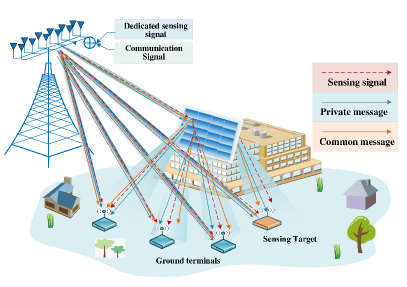
As shown in Fig. 1, a STAR-RIS-enabled downlink ISAC system with RSMA transmission is examined. Specifically, the ISAC BS is configured with $N$ transmit antennas and $N$ receive antennas with half-wavelength spacing, which are arranged in the form of uniform linear arrays (ULAs). This BS not only transmits information to multiple GTs but also is able to detect one target 111 In this paper, we focus on a single target. For scenarios involving multiple targets, a time division (TD) sensing scheme can be utilized. By sequentially sensing each target in distinct, orthogonal time slots, it becomes feasible to utilize all the elements of STAR-RIS to concentrate the beam pattern exclusively towards on a target at any particular moment. The interference among different targets can be prevented. The scenario of single-target sensing can be regarded as a special case of multi-target sensing with the TD sensing approach. through multi-antenna beamforming. Furthermore, to overcome the limitations imposed by traditional RISs in terms of half-space coverage, the STAR-RIS with full-space coverage is employed to coordinate with the BS through a controller for signal enhancement. On the other hand, during downlink transmission, the RSMA scheme is employed to serve $K$ single-antenna GTs with $k\in\{1,2,...,K\}$. The RSMA scheme involves splitting the message transmitted to the $k$-th GT, denoted as $s_{k}$, into two parts: the common (or public) part, denoted as $s_{c,k}$, and the private part, denoted as $s_{{\rm p},k}$. Subsequently, by using a commonly shared codebook, the common components of all GTs $\{s_{c,1},s_{c,2},...,s_{c,K}\}$ are combined into a common stream $s_{c}$, while the beamforming vector for the common stream $s_{c}$ is denoted as $\bm{\varpi}_{c}\in\mathbb{C}^{N\times 1}$. The private part of $k$-th GT is encoded using a private codebook known exclusively by the BS and itself, and the beamforming vector associated with the private message of $k$-th GT is denoted as $\bm{\varpi}_{{\rm p},k}\in\mathbb{C}^{N\times 1}$. Moreover, the dedicated radar signal transmitted for sensing the target is $s_{0}$ with beamforming vector denoted as $\bm{\varpi}_{0}\in\mathbb{C}^{N\times 1}$.

II-B Transmission Model

The STAR-RIS encompasses ${\bm{M}}$ elements capable of both transmission and reflection. Each element engages the ES mode to split incoming signals into two segments, subsequently redirecting them towards the transmission and reflection spaces to perform their respective communication and sensing tasks. The transmission (t) and reflection (r) coefficient matrices of STAR-RIS are represented as

$\displaystyle\bm{\Phi}_{p}=\mathrm{diag}\left({\sqrt{\beta_{1}^{p}}e^{\,j\theta_{1}^{p}},\sqrt{\beta_{2}^{p}}e^{\,j\theta_{2}^{p}},\ldots,\sqrt{\beta_{M}^{p}}e^{\,j\theta_{M}^{p}}}\right),$ (1)
$\displaystyle~{}\forall~{}p\in\{\rm t,r\}$

where $\sqrt{\beta_{m}^{p}}\in[0,1]$ signifies the amplitude and ${\theta_{m}^{p}}\in[0,2\pi)$ signifies the phase-shift value of the $m$-th STAR-RIS element with $m\in\{1,2,...,M\}$. To uphold the principle of energy conservation [20], the amplitude adjustments of all STAR-RIS elements should meet specific criteria, i.e., ${\beta_{m}^{\rm t}}+{\beta_{m}^{\rm r}}$ = 1. We consider that the GTs are stationed on the front face of STAR-RIS, receiving the reflected signals, whereas the target is positioned on the rear side of STAR-RIS, capturing the transmitted signals. With both the direct link and STAR-RIS link considered, the received signal at the $k$-th GT can be represented as

$\displaystyle{y_{k}}$ $\displaystyle=\left({\bm{h}}_{{\rm b}k}^{H}+{\bm{h}}_{{\rm r}k}^{H}\bm{\Phi}_{\rm r}{\bm{H}}_{{\rm br}}^{H}\right){\bm{\varpi}_{c}s_{c}}$ (2)
$\displaystyle+\left({\bm{h}}_{{\rm b}k}^{H}+{\bm{h}}_{{\rm r}k}^{H}\bm{\Phi}_{\rm r}\bm{H}_{{\rm br}}^{H}\right)\sum\nolimits_{k=1}^{K}\bm{\varpi}_{{\rm p},k}s_{{\rm p},k}$
$\displaystyle+\left({\bm{h}}_{{\rm b}k}^{H}+{\bm{h}}_{{\rm r}k}^{H}\bm{\Phi}_{\rm r}\bm{H}_{{\rm br}}^{H}\right)\bm{\varpi}_{0}s_{0}+n_{k},$

where ${\bm{h}}_{{\rm b}k}\in\mathbb{C}^{N\times 1}$ represents the communication channel from BS to $k$-th GT, ${\bm{h}}_{{\rm r}k}\in\mathbb{C}^{M\times 1}$ signifies the communication channel linking STAR-RIS to $k$-th GT, and $\bm{H}_{{\rm br}}\in\mathbb{C}^{N\times M}$ represents the communication link from BS to STAR-RIS. Besides, $\bm{\Phi}_{\rm r}$ indicates the reflecting coefficient matrix associated with the STAR-RIS, $n_{k}$ stands for the additive white Gaussian noise (AWGN) with the power of $\sigma_{k}^{2}$ at $k$-th GT. For GTs, they should firstly decode common message $s_{c}$ by sharing the commonly code-book among GTs, where the private message and sensing signal are treated as interference. Thus, by defining ${\bm{h}}_{k}={\bm{h}}_{{\rm b}k}+\bm{H}_{{\rm br}}{\bm{\Phi}_{\rm r}}{\bm{h}}_{{\rm r}k}$, the achievable rate for GT $k$ to decode common message $s_{c}$ is expressed as

$\displaystyle R_{c,k}=\log_{2}\left(1+\frac{\left|{\bm{h}}_{k}^{H}\bm{\varpi}_{c}\right|^{2}}{\sum\limits_{i=1}^{K}\left|{\bm{h}}_{k}^{H}{\bm{\varpi}_{{\rm p},i}}\right|^{2}+\left|{\bm{h}}_{k}^{H}\bm{\varpi}_{0}\right|^{2}+\sigma_{k}^{2}}\right).$ (3)

Subsequently, the common message is subtracted from the received signal $y_{k}$ through SIC, ensuring that private messages are able to be decoded independently, avoiding by interference from the common message. Therefore, the attainable rate for GT $k$ to decode its designated private message $s_{{\rm p},k}$ is determined as follows:

$\displaystyle R_{{\rm p},k}=\log_{2}\left(1+\frac{\left|{\bm{h}}_{k}^{H}{\bm{\varpi}_{{\rm p},k}}\right|^{2}}{\sum\nolimits_{j\neq k}^{K}\left|{\bm{h}}_{k}^{H}{\bm{\varpi}_{{\rm p},j}}\right|^{2}+\left|{\bm{h}}_{k}^{H}\bm{\varpi}_{0}\right|^{2}+\sigma_{k}^{2}}\right).$ (4)

Furthermore, to ensure successfully decoding of common messages by all GTs, the achievable rates for each GT should exceed the allocated data rates [28]. This implies that, for every GT to accurately detect its designated information from the common message, the following constraint should be fulfilled, i.e.,

$\displaystyle\sum\nolimits_{k=1}^{K}c_{k}\leq R_{c},~{}R_{c}=\min\{R_{c,1},R_{c,2},...,R_{c,K}\},$ (5)

where $c_{k}$ represents the actual data rate assigned to $k$-th GT.

II-C Sensing Model

The ISAC signals emitted by the BS initially arrive at the detection target through both the direct link and the refractive path facilitated by STAR-RIS. Subsequently, the echo signal, upon reflection from the target, traverse similar paths back to the BS. By defining ${\bm{h}}_{\rm bt}\in\mathbb{C}^{N\times 1}$ and ${\bm{h}}_{\rm rt}\in\mathbb{C}^{M\times 1}$ as the channel links connecting the BS to target, and the STAR-RIS to target, respectively, and $\bm{\Phi}_{\rm t}$ as the transmission coefficient matrix associated with STAR-RIS, the echo signal reflected by the target and $I$ scatters is represented as

$\displaystyle{\bm{y}}_{\rm bs}=({\bm{h}}_{\rm bt}+{\bm{H}}_{\rm br}\bm{\Phi}_{\rm t}{\bm{h}}_{\rm rt})({\bm{h}}_{\rm bt}+{\bm{H}}_{\rm br}\bm{\Phi}_{\rm t}{\bm{h}}_{\rm rt})^{H}{\bm{A}}(\theta_{0})\times$ (6)
$\displaystyle(\sum\nolimits_{k=1}^{K}\bm{\varpi}_{{\rm p},k}s_{{\rm p},k}+{\bm{\varpi}_{c}s_{c}}+\bm{\varpi}_{0}s_{0})+{\sum\nolimits_{i=1}^{I}{\bm{z}}_{i}}+{\bm{n}}_{s},$

where the intended target for detection is located at an angle of $\theta_{0}$, and ${\bf A}(\theta_{0})=\beta_{0}{\bm{a}}(\theta_{0}){\bm{a}}(\theta_{0})^{H}$ with ${\bm{a}}(\theta_{0})\triangleq[1,e^{j\pi\sin(\theta_{0})},...,e^{j\pi(N-1)\sin(\theta_{0})}]^{T}$ denoting as the steering vector of the antenna array at the BS [29]. Besides, $\beta_{0}\in\mathbb{C}$ denotes the complex reflection factor, ${\bm{z}}_{i}\in\mathbb{C}^{N\times 1}$ represents the undesired single-independent interference from $I$ uncorrelated scatters positioned at angles $\{\theta_{i}\}\sum\nolimits_{i=1}^{I}$ with $\theta_{i}\neq\theta_{0}$ and $i\in\{1,...,I\}$, ${\bm{n}}_{s}\in\mathbb{C}^{N\times 1}$ denotes the AWGN at the BS with ${\bm{n}}_{s}\sim\mathcal{CN}(0,\sigma_{s}^{2}\bm{I}_{N})$. By defining ${\bm{h}}_{\rm t}={\bm{h}}_{\rm bt}+{\bm{H}}_{\rm br}\bm{\Phi}_{\rm t}{\bm{h}}_{\rm rt}$, the output sensing SINR is given by

$\displaystyle\gamma_{\rm bs}=\frac{\|{\bm{h}}_{\rm t}\|^{2}{\rm Tr}\left({\bm{h}}_{\rm t}{\bm{h}}_{\rm t}^{H}{\bf A}(\theta_{0}){\bf Q}{\bf A}(\theta_{0})^{H}\right)}{{\rm Tr}\left(\sum\nolimits_{i=1}^{I}\|{\bm{h}}_{i}\|^{2}{\bm{h}}_{i}{\bm{h}}_{i}^{H}{\bf A}(\theta_{i}){\bf Q}{\bf A}(\theta_{i})^{H}+\sigma_{s}^{2}{\bf I}_{N}\right)},$ (7)

where ${\bf Q}$ = ${\bm{\varpi}}_{c}{\bm{\varpi}}_{c}^{H}$ + $\sum\nolimits_{k=1}^{K}{\bm{\varpi}_{{\rm p},k}}{\bm{\varpi}_{{\rm p},k}}^{H}$ + ${\bm{\varpi}}_{0}{\bm{\varpi}}_{0}^{H}$. Moreover, ${\bm{h}}_{i}$ = ${\bm{h}}_{\rm bi}+{\bm{H}}_{\rm br}\bm{\Phi}_{\rm t}{\bm{h}}_{\rm ri}$, where ${\bm{h}}_{\rm bi}$ and ${\bm{h}}_{\rm ri}$ are the communication channel connecting the BS to $i$-th scatter and the communication link connecting STAR-RIS to $i$-th scatter.

III Problem formulation and proposed solution

III-A Problem Formulation

To maximize the sensing SINR while ensuring the communication rate requirements of all GTs can be guaranteed, an optimization problem is formulated by simultaneously optimizing the transmit beamforming vectors of the BS $\{\bm{\varpi}_{c},\bm{\varpi}_{{\rm p},k},\bm{\varpi}_{0}\}$, alongside the transmission and reflection beamforming matrices $\{{\bm{\Phi}}_{\rm t},{\bm{\Phi}}_{\rm r}\}$, and the rate allocation vector $c_{k}$ for the common stream. Specifically, the sensing SINR maximization problem is mathematically modeled by

$\displaystyle\textbf{P}_{\textbf{A}}:\mathop{\max}\limits_{\bm{\varpi}_{c},\bm{\varpi}_{{\rm p},k},\bm{\varpi}_{0},c_{k},{\bm{\Phi}}_{\rm t},{\bm{\Phi}}_{\rm r}}{\kern 1.0pt}\gamma_{\rm bs}$
$\displaystyle{\rm{s.}}{\rm{t.}}$ $\displaystyle~{}{\rm Tr}(\bm{\varpi}_{c}\bm{\varpi}_{c}^{H})+{\rm Tr}(\sum\nolimits_{k=1}^{K}{\bm{\varpi}}_{{\rm p},k}{\bm{\varpi}}_{{\rm p},k}^{H})$
$\displaystyle+{\rm Tr}({\bm{\varpi}}_{0}{\bm{\varpi}}_{0}^{H})\leq P_{\max},$ (8a)
$\displaystyle~{}\sum\nolimits_{k=1}^{K}c_{k}\leq R_{c},R_{c}=\min\{R_{c,1},R_{c,2},...,R_{c,K}\},$ (8b)
$\displaystyle~{}c_{k}+R_{p,k}\geq R_{k}^{\rm th},$ (8c)
$\displaystyle~{}c_{k}\geq 0,~{}\forall~{}k\in\{1,...,K\},$ (8d)
$\displaystyle~{}{\beta_{m}^{\rm t}}+{\beta_{m}^{\rm r}}=1,~{}\forall~{}m\in\{1,...,M\},$ (8e)
$\displaystyle~{}\sqrt{\beta_{m}^{p}}\in[0,1],~{}\theta_{m}^{p}\in[0,2\pi),~{}~{}p\in\{\rm t,r\},$ (8f)

where (8a) is the transmit power constraint with $P_{\max}$ being the maximum available power at the BS. Constraint (8b) signifies that the total actual rate assigned to the GTs must not exceed the attainable common-stream rate among all GTs. (8c) is the minimum rate requirement for each GT with $R_{k}^{\rm th}$ being the rate threshold of $k$-th GT. (8e) signifies that, owing to passive characteristics of STAR-RIS, the amplitude responses of all elements are confined by the principle of energy conservation. (8f) represents the permissible range of the transmission coefficients (TCs) and reflection coefficients (RCs) of STAR-RIS elements, respectively. It should be noted that the beamforming vectors $\{\bm{\varpi}_{c},\bm{\varpi}_{{\rm p},k},\bm{\varpi}_{0}\}$ and the TCs and RCs $\{{\bm{\Phi}}_{\rm t},{\bm{\Phi}}_{\rm r}\}$ are multiply coupled together in the optimization objective and in constraints (8b) and (8c). Consequently, problem $\textbf{P}_{\textbf{A}}$ is non-convex. Hence, we intend to utilize the SDR, MM, and SROCR methods to devise the successive convex approximation (SCA)-based iterative algorithm, which is capable of finding the solution of $\textbf{P}_{\textbf{A}}$.

III-B Proposed Algorithm

In this section, we present the SCA-based iterative algorithm aimed at solving the formulated problem. Initially, as the matrices of TCs and RCs are coupled with the variables associated with transmit beamforming and the actual data rate assigned to each GT, the initial problem $\textbf{P}_{\textbf{A}}$ is split into two sub-problems. Firstly, with given initial value of TCs and RCs $\{{\bm{\Phi}}_{\rm t}^{(l)},{\bm{\Phi}}_{\rm r}^{(l)}\}$, the first sub-problem $\textbf{P}_{\textbf{B1}}$ w.r.t. the transmit beamforming vectors and the real data rate allocation is successively tackled by implementing Dinkelbach’s transform, SDR, first-order Taylor expansion and variable substitution. Secondly, building upon the solution acquired through solving $\textbf{P}_{\textbf{B1}}$, the second sub-problem $\textbf{P}_{\textbf{B2}}$ w.r.t. the TCs and RCs of STAR-RIS is tackled by utilizing the SDR, MM and the SROCR methods. Finally, the overall solution for the original problem is derived by iteratively solving two sub-problems.

To obtain a tractable solution method, a classic SDR-based approach is applied. Specifically, by applying the equivalent transformation of ${\bf W}_{c}$ = ${\bm{\varpi}}_{c}{\bm{\varpi}}_{c}^{H}$, ${\bf W}_{{\rm p},k}={\bm{\varpi}}_{{\rm p},k}{\bm{\varpi}}_{{\rm p},k}^{H}$, ${\bf W}_{0}={\bm{\varpi}}_{0}{\bm{\varpi}}_{0}^{H}$, with given ${\bf H}_{k}={\bm{h}}_{k}{\bm{h}}_{k}^{H}$ and $\{{\bm{\Phi}}_{\rm t}^{(l)}$, ${\bm{\Phi}}_{\rm r}^{(l)}\}$, the subproblem $\textbf{P}_{\textbf{B1}}$ w.r.t. $\{{\bf W}_{c},{\bf W}_{{\rm p},k}$,${\bf W}_{0},c_{k}\}$ is given by

$\displaystyle\textbf{P}_{\textbf{B1}}:\mathop{\max}\limits_{{\bf W}_{c},{\bf W}_{{\rm p},k},{\bf W}_{0},c_{k}}{\kern 1.0pt}\gamma_{\rm bs}$
$\displaystyle{\rm{s.}}{\rm{t.}}$ $\displaystyle~{}{\rm Tr}({\bf W}_{c}+{\bf W}_{{\rm p},k}+{\bf W}_{0})\leq P_{\max},$ (9a)
$\displaystyle{\rm rank}({\bf W}_{c})=1,{\rm rank}({\bf W}_{{\rm p},k})=1,{\rm rank}({\bf W}_{0})=1,$ (9b)
$\displaystyle{\bf W}_{{\rm p},k}\succeq 0,~{}{\bf W}_{c}\succeq 0,~{}{\bf W}_{0}\succeq 0,$ (9c)
$\displaystyle\sum\limits_{k=1}^{K}c_{k}\leq\mathop{\min}\limits_{\forall k}\log_{2}(1+\tfrac{{\rm Tr}({\bf H}_{k}{\bf W}_{c})}{\sum\limits_{i=1}^{K}{\rm Tr}({\bf H}_{k}({\bf W}_{{\rm p},i}+{\bf W}_{0}))+\sigma_{k}^{2}}),$ (9d)
$\displaystyle c_{k}+\log_{2}(1+\tfrac{{\rm Tr}({\bf H}_{k}{\bf W}_{{\rm p},k})}{\sum\limits_{j\neq k}^{K}{\rm Tr}({\bf H}_{k}{\bf W}_{{\rm p},j}+{\bf H}_{k}{\bf W}_{0})+\sigma_{k}^{2}})\geq R_{k}^{\rm th}.$ (9e)
Theorem 1.

If the optimized beamforming vectors for sub-problem ${\mathbf{P}}_{\textbf{B1}}$ is denoted as $\{\widehat{{\bf W}}_{c},\widehat{{\bf W}}_{p,k},\widehat{{\bf W}}_{0}\}$, there always exists another set of solutions $\{\overline{{\bf W}}_{c},\overline{{\bf W}}_{p,k},\overline{{\bf W}}_{0}\}$. It can achieve same system performance not inferior to that of $\{\widehat{{\bf W}}_{c},\widehat{{\bf W}}_{p,k},\widehat{{\bf W}}_{0}\}$, where

$\displaystyle\overline{{\bf W}}_{c}=\widehat{{\bf W}}_{c}+\zeta_{c}\widehat{{\bf W}}_{0},~{}\overline{{\bf W}}_{p,k}=\widehat{{\bf W}}_{p,k}+\zeta_{k}\widehat{{\bf W}}_{0},$ (10)
$\displaystyle\overline{{\bf W}}_{0}=0,~{}~{}\zeta_{c}+\sum\nolimits_{k=1}^{K}\zeta_{k}=1.$
Proof:

See Appendix A. ∎

From Theorem 1, we can observe that the optimization variable ${\bf W}_{0}$ is unnecessary. It also reveals that when the BS only transmits communication waveforms, it can achieve the same sensing SINR as when transmitting a combination of communication and dedicated sensing waveforms, which is verified by our simulation results in Section IV. In other words, in each iteration, an optimal solution obtained under the combined waveform assumption can always be equivalently transformed into those corresponding to the communication-only waveform assumption, and this transformation is independent of the transmission and reflection beamforming design at the STAR-RIS. Therefore, the optimization variables of ${\bf W}_{0}$ can be eliminated to offer a simplified optimization form of problem ${\mathbf{P}}_{\textbf{B1}}$.

However, the simplified problem is still non-convex. In the following part, we apply Dinkelbach’s transform, SDR, first-order Taylor expansion to deal with non-convex objective and constraints. Firstly, the achievable rate for GT $k$ to decode common message is re-expressed as

$\displaystyle R_{c,k}=\log_{2}\left(1+\frac{{\rm Tr}({\bf H}_{k}{\bf W}_{c})}{\sum\nolimits_{i=1}^{K}{\rm Tr}({\bf H}_{k}{\bf W}_{{\rm p},i})+\sigma_{k}^{2}}\right).$ (11)

To address the non-convex constraint (9d), we introduce a slack variable ${a}_{k}$ and impose additional inequality constraints, thereby transforming it into the convex one, i.e.,

$\displaystyle\rho_{k}{\rm Tr}\left({\bf H}_{k}({\bf W}_{c}+\sum\nolimits_{i=1}^{K}{\bf W}_{{\rm p},i})\right)+1\geq 2^{a_{k}},$ (12)

and

$\displaystyle 2^{a_{k}-{(\sum\nolimits_{k=1}^{K}c_{k})}}\geq{\rho_{k}{\rm Tr}\left({\bf H}_{k}(\sum\nolimits_{i=1}^{K}{\bf W}_{{\rm p},i})\right)+1},$ (13)

with $\rho_{k}=\tfrac{1}{\sigma_{k}^{2}}$. Nevertheless, since constraint (13) continues to be non-convex, the first-order Taylor expansion is utilized to tackle it. Given feasible solution $\{{a_{k}}^{(l)},{c_{k}}^{(l)}\}$, it fulfills the condition that

$\displaystyle 2^{{a_{k}}^{(l)}-\sum\nolimits_{k=1}^{K}{c_{k}}^{(l)}}+\ln 2(2^{{a_{k}}^{(l)}-\sum\nolimits_{k=1}^{K}{c_{k}}^{(l)}})(a_{k}-{a_{k}}^{(l)})$ (14)
$\displaystyle-\ln 2(2^{{a_{k}}^{(l)}-\sum\nolimits_{k=1}^{K}{c}_{k}^{(l)}})(\sum\nolimits_{k=1}^{K}c_{k}-\sum\nolimits_{k=1}^{K}{c_{k}^{(l)}})\geq$
$\displaystyle{\rho_{k}{\rm Tr}\left({\bf H}_{k}(\sum\nolimits_{i=1}^{K}{\bf W}_{{\rm p},i})\right)+1}.$

Similarly, for non-convex constraint (9e), by introducing auxiliary variable $b_{k}$, we can convert it into the equivalent inequality constraints as follows,

$\displaystyle{\rho_{k}{\rm Tr}\left({\bf H}_{k}(\sum\nolimits_{i=1}^{K}{\bf W}_{{\rm p},i})\right)+1}\geq 2^{b_{k}},$ (15)

and

$\displaystyle 2^{b_{k}+c_{k}-R_{\rm th}^{k}}\geq{\rho_{k}{\rm Tr}\left({\bf H}_{k}(\sum\nolimits_{j\neq k}^{K}{\bf W}_{{\rm p},j})\right)+1}.$ (16)

With the first-order Taylor expansion employed, the (16) is reexpressed as

$\displaystyle 2^{{b_{k}}^{(l)}+{c_{k}}^{(l)}-R_{\rm th}^{k}}+\ln 2(2^{{b_{k}^{(l)}}+{c_{k}^{(l)}}-R_{\rm th}^{k}})(b_{k}+c_{k}-{b_{k}^{(l)}}-{c_{k}^{(l)}})\geq$ (17)
$\displaystyle{\rho_{k}{\rm Tr}\left({\bf H}_{k}(\sum\nolimits_{j\neq k}^{K}{\bf W}_{{\rm p},j})\right)+1}.$

Moreover, by defining ${\bf Q}={\bf W}_{c}+\sum\nolimits_{i=1}^{K}{\bf W}_{{\rm p},i}$, ${\bf H}_{t}={\bf h}_{t}{\bf h}_{t}^{H}$ and ${\bf A}(\theta_{i})=\beta_{i}{\bm{a}}(\theta_{i}){\bm{a}}(\theta_{i})^{H}$, ${\bf H}_{i}={\bm{h}}_{i}{\bm{h}}_{i}^{H}$, the numerator and denominator of equation (7) are rewritten as ${\bf A}_{t}$ and (${\bf B}_{t}+{\bf I}_{N})$, respectively, where ${\bf A}_{t}$ and ${\bf B}_{t}$ are given by

$\displaystyle{\bf A}_{t}=\gamma_{0}{\bf H}_{t}{\bf H}_{t}^{H}{\bf A}(\theta_{0}){\bf Q}{\bf A}(\theta_{0})^{H},$ (18)

and

$\displaystyle{\bf B}_{t}=\sum\nolimits_{i=1}^{I}\gamma_{i}{\bf H}_{i}{\bf H}_{i}^{H}{\bf A}(\theta_{i}){\bf Q}{\bf A}(\theta_{i})^{H},$ (19)

with $\gamma_{i}=\frac{1}{\sigma_{s}^{2}}$ and $i\in\{0,1,...,I\}$. To sum up, the optimization objective $\gamma_{\rm bs}$ can be re-expressed as

$\displaystyle\gamma_{\rm bs}=\frac{{\rm Tr}({\bf A}_{t})}{{\rm Tr}({\bf B}_{t}+{\bf I}_{N})}.$ (20)

Unfortunately, the expression in (20) continues to be non-convex because of the fractional objective and the ambiguity functions w.r.t. ${\bf Q}$. To resolve these challenges, the fractional objective is reshaped through the application of Dinkelbach’s transform, subsequently converting the problem into an explicit form w.r.t. ${\bf Q}$ [30]. Explicitly, by incorporating a new auxiliary variable $\omega$, the objective function is converted into an alternative form, which is given by

$\displaystyle\min\limits_{\bf Q}~{}\omega{{\rm Tr}({\bf B}_{t}+{\bf I}_{N})}-{{\rm Tr}({\bf A}_{t})},$ (21)

where $\omega=\frac{{{\rm Tr}({\bf A}_{t}^{(l)})}}{{\rm Tr}({\bf B}_{t}^{(l)}+{\bf I}_{N})}$. Furthermore, for the rank-one constraints of ${\rm rank}({\bf W}_{c})=1$ and ${\rm rank}({\bf W}_{{\rm p},k})=1$, the SROCR-based method is utilized to obtain locally optimal rank-one solutions [31]. The specific step is to restrict the ratio of the largest eigenvalue to the trace of ${{\bf W}_{c}}$ through a flexible parameter $\tau_{c}$ ranging from 0 to 1, so that the rank-one constraint can be substituted with

$\displaystyle{\bf u}_{\rm max}\left({\bf W}_{c}\right)^{H}{\bf W}_{c}{\bf u}_{\rm max}\left({\bf W}_{c}\right)\geq\tau_{c}{\rm Tr}({\bf W}_{c}),$ (22)

where

$\displaystyle\tau_{c}^{(l)}=\min\left(1,\tfrac{{\bf e}_{\rm max}\left({\bf W}_{c}^{(l)}\right)}{{\rm Tr}({\bf W}_{c}^{(l)})}+\delta_{c}^{(l)}\right),$ (23a)
$\displaystyle\delta_{c}^{(l)}\in\{0,1-\tfrac{{\bf e}_{\rm max}\left({\bf W}_{c}^{(l)}\right)}{{\rm Tr}({\bf W}_{c}^{(l)})}\}.$ (23b)

Besides, ${\bf u}_{\rm max}\left({\bf W}_{c}\right)$ is the largest eigenvector of matrix ${\bf W}_{c}$, and ${\bf e}_{\rm max}\left({\bf W}_{c}\right)$ is the largest eigenvalue of matrix ${\bf W}_{c}$. With a similar manner, the other rank-one constraint of ${\rm rank}({\bf W}_{{\rm p},k})=1$ can also be converted into processable forms. After a series of transformations, the sub-problem ${\mathbf{P}}_{\textbf{B1}}$ can be rewritten as

$\displaystyle{{\mathbf{P}}_{\textbf{B1-1}}:}\min\limits_{\left\{{{\bf W}_{c},{\bf W}_{{\rm p},k},c_{k},a_{k},b_{k}}\right\}}\omega{{\rm Tr}({\bf B}_{t}+{\bf I}_{N})}-{{\rm Tr}({\bf A}_{t})}$
s.t.(12),(LABEL:rate_k_fenmu_common),(15),(LABEL:rate_fenmu_private),formulae-sequencest12LABEL:rate_k_fenmu_common15LABEL:rate_fenmu_private\displaystyle{\mathrm{s.t.}}~{}(\ref{rate_k_fenzi}),(\ref{rate_k_fenmu_common}),(\ref{rate_k_fenz_private}),(\ref{rate_fenmu_private}),
$\displaystyle{\rm Tr}({\bf W}_{c}+\sum\nolimits_{k=1}^{K}{\bf W}_{{\rm p},k})\leq P_{\max},$ (24a)
$\displaystyle{\bf u}_{\rm max}({\bf W}_{c}^{(l)})^{H}{\bf W}_{c}{\bf u}_{\rm max}({\bf W}_{c}^{(l)})\geq\tau_{c}^{(l)}{\rm Tr}({\bf W}_{c}),$ (24b)
$\displaystyle{\bf u}_{\rm max}({\bf W}_{{\rm p},k}^{(l)})^{H}{\bf W}_{{\rm p},k}{\bf u}_{\rm max}({\bf W}_{{\rm p},k}^{(l)})\geq\tau_{k}^{(l)}{\rm Tr}({\bf W}_{{\rm p},k}),$ (24c)
$\displaystyle{\bf W}_{{\rm p},k}\succeq 0,~{}{\bf W}_{c}\succeq 0,~{}$ (24d)

where ${\bf W}_{c}^{(l)}$ and ${\bf W}_{{\rm p},k}^{(l)}$ represent the optimal solutions of the $l$-th iteration, (24b) and (24c) are the relaxed convex constraints for tackling rank-one constraints, respectively. So far, ${\mathbf{P}}_{\textbf{B1-1}}$ is a convex problem, which can be solved by using the following Algorithm 1.

Algorithm 1 Iterative algorithm for solving problem ${\mathbf{P}}_{\textbf{B1-1}}$
1:  Initialize iteration index $l$ = 0, ${a_{k}}^{(l)}$, ${b_{k}}^{(l)}$, ${c_{k}}^{(l)}$, ${\bf W}_{c}^{(l)}$, ${\bf W}_{{\rm p},k}^{(l)}$, $\tau_{c}^{(l)}$, $\tau_{k}^{(l)}$,and calculate $\omega^{(l)}$;
2:  Initialize $\bm{\Phi}_{\rm t}^{(l)}$ and $\bm{\Phi}_{\rm r}^{(l)}$;
3:  Define initial step sizes:     $\delta_{c}^{(l)}\in\{0,1-{{\bf e}_{\rm max}({\bf W}_{c}^{(l)})}/{{\rm Tr}({\bf W}_{c}^{(l)})}\}$,     $\delta_{k}^{(l)}\in\{0,1-{{\bf e}_{\rm max}({\bf W}_{{\rm p},k}^{(l)})}/{{\rm Tr}({\bf W}_{{\rm p},k}^{(l)})}\}$;
4:  repeat
5:     Solve problem $\textbf{P}_{\textbf{B1-1}}$ with $\tau_{c}^{(l)}$, $\tau_{k}^{(l)}$, $\omega^{(l)}$, $\bm{\Phi}_{\rm t}^{(l)}$ and $\bm{\Phi}_{\rm r}^{(l)}$;
6:     if problem $\textbf{P}_{\textbf{B1-1}}$ is solvable  then
7:        Obtain optimal ${\bf W}_{c}^{*}$, ${\bf W}_{{\rm p},k}^{*}$, ${a_{k}}^{*}$, ${b_{k}}^{*}$, ${c_{k}}^{*}$,
8:        $\delta_{c}^{(l+1)}=\delta_{c}^{(l)}$, $\delta_{k}^{(l+1)}=\delta_{k}^{(l)}$,
9:     else
10:         ${\bf W}_{c}^{(l+1)}$=${\bf W}_{c}^{(l)}$, ${\bf W}_{{\rm p},k}^{(l+1)}$=${\bf W}_{{\rm p},k}^{(l)}$,$\delta_{c}^{(l+1)}=\delta_{c}^{(l)}/2$, $\delta_{k}^{(l+1)}=\delta_{k}^{(l)}/2$,
11:     end if
12:     $\tau_{c}^{(l+1)}=\min\left(1,\tfrac{{\bf e}_{\rm max}\left({\bf W}_{c}^{(l+1)}\right)}{{\rm Tr}({\bf W}_{c}^{(l+1)})}+\delta_{c}^{(l+1)}\right)$,$\tau_{k}^{(l+1)}=\min\left(1,\tfrac{{\bf e}_{\rm max}\left({\bf W}_{{\rm p},k}^{(l+1)}\right)}{{\rm Tr}({\bf W}_{{\rm p},k}^{(l+1)})}+\delta_{k}^{(l+1)}\right)$,
13:  until  $\lvert 1-\tau_{c}^{(l+1)}\rvert$ $\leq$ $\epsilon_{1}$, $\lvert 1-\tau_{k}^{(l+1)}\rvert$ $\leq$ $\epsilon_{1}$ and the difference between adjacent objective values for $\textbf{P}_{\textbf{B1-1}}$ below $\epsilon_{2}$.

Based on the obtained $\{{\bf W}_{c}^{(l)},{\bf W}_{{\rm p},k}^{(l)},c_{k}\}$ of $\textbf{P}_{\textbf{B1-1}}$, the sub-problem w.r.t. $\{{\bm{\Phi}}_{\rm t},{\bm{\Phi}}_{\rm r}\}$ will be solved in the following part. Firstly, as the optimization variables ${\bm{\Phi}}_{\rm t}$ and ${\bm{\Phi}}_{\rm r}$ are comprised in the expression of transmission channel, we may attempt to extract variable ${\bm{\Phi}}_{\rm t}$ and ${\bm{\Phi}}_{\rm r}$ from the channel expression ${\bm{h}}_{\rm t}$ and ${\bm{h}}_{k}$, respectively. By defining ${\bm{\nu}}_{t}=[\sqrt{\beta_{1}^{t}}e^{j\theta_{1}^{t}},\sqrt{\beta_{2}^{t}}e^{j\theta_{2}^{t}},...,\sqrt{\beta_{M}^{t}}e^{j\theta_{M}^{t}},1]^{T}$, the following transformation is obtained, i.e., ${\bm{h}}_{\rm t}=[{\bm{H}}_{\rm br}{\rm diag}({\bm{h}}_{\rm rt}),{\bm{h}}_{\rm bt}]{\bm{\nu}}_{t}$. Therefore, ${\bf A}_{t}$ shown in (18) can be reformulated as

$\displaystyle{\bf A}_{t}=\gamma_{t}{\bm{\nu}}_{t}^{H}{\bf A_{1}}{\bm{\nu}}_{t}{\bm{\nu}}_{t}^{H}{\bf B_{1}}{\bm{\nu}}_{t}$ (25)
$\displaystyle=\gamma_{t}{{\rm Tr}({\bf A_{1}}{\bm{\nu}}_{t}{\bm{\nu}}_{t}^{H}{\bf B_{1}}{\bm{\nu}}_{t}{\bm{\nu}}_{t}^{H}})$
$\displaystyle\overset{(a)}{=}\gamma_{t}\widehat{{\bm{\nu}}}_{t}^{H}({\bf B_{1}}^{T}\otimes{\bf A_{1}})\widehat{{\bm{\nu}}}_{t},$

where $\widehat{{\bm{\nu}}}_{t}={\rm vec}({\bm{\nu}}_{t}{\bm{\nu}}_{t}^{H})$, and step $(a)$ is well-founded due to the application of the identity ${\rm Tr}({\bf EXFX})={\rm vec}({\bf X})^{H}({\bf F}^{T}\otimes{\bf E}){\rm vec}(\bf X)$, ${\bf A_{1}}$ and ${\bf B_{1}}$ are defined in (LABEL:A1B1).

$\displaystyle{\bf A_{1}}=\begin{bmatrix}{\rm diag}^{H}({\bm{h}}_{\rm rt}){\bm{H}}_{\rm br}^{H}{\bm{H}}_{\rm br}{\rm diag}({\bm{h}}_{\rm rt}),&{\rm diag}^{H}({\bm{h}}_{\rm rt}){\bm{H}}_{\rm br}^{H}{\bm{h}}_{\rm bt}\\ {\bm{h}}_{\rm bt}^{H}{\bm{H}}_{\rm br}{\rm diag}({\bm{h}}_{\rm rt}),&{\bm{h}}_{\rm bt}^{H}{\bm{h}}_{\rm bt}\end{bmatrix},$ (26)
$\displaystyle{\bf B_{1}}=\begin{bmatrix}{\rm diag}^{H}({\bm{h}}_{\rm rt}){\bm{H}}_{\rm br}^{H}{\bf Q}{\bm{H}}_{\rm br}{\rm diag}({\bm{h}}_{\rm rt}),&{\rm diag}^{H}({\bm{h}}_{\rm rt}){\bm{H}}_{\rm br}^{H}{\bf Q}{\bm{h}}_{\rm bt}\\ {\bm{h}}_{\rm bt}^{H}{\bf Q}{\bm{H}}_{\rm br}{\rm diag}({\bm{h}}_{\rm rt}),&{\bm{h}}_{\rm bt}^{H}{\bf Q}{\bm{h}}_{\rm bt}\end{bmatrix},$
$\displaystyle{\bf A_{i1}}=\begin{bmatrix}{\rm diag}^{H}({\bm{h}}_{\rm ri}){\bm{H}}_{\rm br}^{H}{\bm{H}}_{\rm br}{\rm diag}({\bm{h}}_{\rm ri}),&{\rm diag}^{H}({\bm{h}}_{\rm ri}){\bf H}_{\rm br}^{H}{\bm{h}}_{\rm bi}\\ {\bm{h}}_{\rm bi}^{H}{\bm{H}}_{\rm br}{\rm diag}({\bm{h}}_{\rm ri}),&{\bm{h}}_{\rm bi}^{H}{\bm{h}}_{\rm bi}\end{bmatrix},$
$\displaystyle{\bf B_{i1}}=\begin{bmatrix}{\rm diag}^{H}({\bm{h}}_{\rm ri}){\bm{H}}_{\rm br}^{H}{\bf Q}{\bm{H}}_{\rm br}{\rm diag}({\bm{h}}_{\rm ri}),&{\rm diag}^{H}({\bm{h}}_{\rm ri}){\bm{H}}_{\rm br}^{H}{\bf Q}{\bm{h}}_{\rm bi}\\ {\bm{h}}_{\rm bi}^{H}{\bf Q}{\bm{H}}_{\rm br}{\rm diag}({\bm{h}}_{\rm ri}),&{\bm{h}}_{\rm bi}^{H}{\bf Q}{\bm{h}}_{\rm bi}\end{bmatrix}.$


By using the same derivation method, ${\bf B}_{t}$ shown in (19) is given as

$\displaystyle{\bf B}_{t}=\sum\nolimits_{i=1}^{I}\gamma_{i}{\rm Tr}({\bf A_{i1}}{\bm{\nu}}_{t}{\bm{\nu}}_{t}^{H}{\bf B_{i1}}{\bm{\nu}}_{t}{\bm{\nu}}_{t}^{H})$ (27)
$\displaystyle\overset{(a)}{=}\sum\nolimits_{i=1}^{I}\gamma_{i}\widehat{{\bm{\nu}}}_{t}^{H}({\bf B_{i1}}^{T}\otimes{\bf A_{i1}})\widehat{{\bm{\nu}}}_{t},$

where ${\bf A_{i1}}$ and ${\bf B_{i1}}$ are also defined in (LABEL:A1B1). Therefore, the optimization objective can be re-arranged as

$\displaystyle\min\limits_{{\bm{\nu}}_{t}}~{}\widehat{{\bm{\nu}}}_{t}^{H}\left(\sum\limits_{i=1}^{I}\omega\gamma_{i}({\bf B_{i1}}^{T}\otimes{\bf A_{i1}})-\gamma_{0}({\bf B_{1}}^{T}\otimes{\bf A_{1}})\right)\widehat{{\bm{\nu}}}_{t}.$ (28)

The existence of the quartic form of optimization variables ${\bm{\nu}}_{t}$ can be noticed in (28). Subsequently, the MM method is utilized to generate an appropriate surrogate function by leveraging a lower bound defined in (29), i.e.,

$\displaystyle\widehat{{\bm{\nu}}}_{t}^{H}{\bf F}\widehat{{\bm{\nu}}}_{t}\approx(\widehat{{\bm{\nu}}}_{t}^{(l)})^{H}({\bf F}+{\bf F}^{H})\widehat{{\bm{\nu}}}_{t}-(\widehat{{\bm{\nu}}}_{t}^{(l)})^{H}{\bf F}(\widehat{{\bm{\nu}}}_{t}^{(l)}),$ (29)

where ${\bf F}=\sum\nolimits_{i=1}^{I}\omega\gamma_{i}({\bf B_{i1}}^{T}\otimes{\bf A_{i1}})-\gamma_{t}({\bf B_{1}}^{T}\otimes{\bf A_{1}})$. However, (29) is a complex-valued convex function. Thus, by defining $\overrightarrow{{{\bm{\nu}}}_{t}}=\begin{bmatrix}\Re\left(\widehat{{\bm{\nu}}}_{t}\right)\\ \Im\left(\widehat{{\bm{\nu}}}_{t}\right)\end{bmatrix}$ and $\overrightarrow{\bf F}=\begin{bmatrix}\Re{(\bf F)},&-\Im{(\bf F)}\\ \Im{(\bf F)},&\Re{(\bf F)}\end{bmatrix}$, we first convert (29) into a real-valued one, i.e.,

$\displaystyle\widehat{{\bm{\nu}}}_{t}^{H}{\bf F}\widehat{{\bm{\nu}}}_{t}$ $\displaystyle=\overrightarrow{{{\bm{\nu}}}_{t}}^{T}\overrightarrow{\bf F}\overrightarrow{{{\bm{\nu}}}_{t}}$ (30)
$\displaystyle\approx 2(\overrightarrow{{{\bm{\nu}}}}_{t}^{(l)})^{T}\overrightarrow{\bf F}\overrightarrow{{{\bm{\nu}}}_{t}}-(\overrightarrow{{\bm{\nu}}}_{t}^{(l)})^{T}\overrightarrow{\bf F}\overrightarrow{{\bm{\nu}}}_{t}^{(l)}.$

Through the executions of multiple complex mathematical manipulations, the first term in (30) can be expressed as

$\displaystyle 2(\overrightarrow{{{\bm{\nu}}}}_{t}^{(l)})^{T}\overrightarrow{\bf F}\overrightarrow{{{\bm{\nu}}}_{t}}=2\Re({\bm{\psi}}^{H}\widehat{{\bm{\nu}}}_{t}),$ (31)

where ${\bm{\psi}}^{H}=\begin{bmatrix}(\overrightarrow{{{\bm{\nu}}}}_{t}^{(l)})^{T}\overrightarrow{\bf F}\end{bmatrix}_{1:M^{2}}-j\begin{bmatrix}(\overrightarrow{{{\bm{\nu}}}}_{t}^{(l)})^{T}\overrightarrow{\bf F}\end{bmatrix}_{M^{2}+1:2M^{2}}$. Besides, based on the fact that $\widehat{{\bm{\nu}}}_{t}={\rm vec}({\bm{\nu}}_{t}{\bm{\nu}}_{t}^{H})$ and ${\rm\bf x^{H}F^{H}x}={\rm vec}^{H}(\bf F){\rm vec}(\rm{\bf xx}^{H})$, we have

$\displaystyle 2\Re({\bm{\psi}}^{H}\widehat{{\bm{\nu}}}_{t})$ $\displaystyle=2\Re({\bm{\nu}}_{t}^{H}(\triangle{\bm{\psi}})^{H}{\bm{\nu}}_{t})$ (32)
$\displaystyle={\bm{\nu}}_{t}^{H}\left(\triangle({\bm{\psi}})+(\triangle({\bm{\psi}}))^{H}\right){\bm{\nu}}_{t},$

where $\triangle(\cdot)$ denotes the inverse operation of matrix vectorization $\rm vec(\cdot)$. Actually, after a series of mathematical transformations, we have $\triangle(\bm{\psi})=\sum\nolimits_{i=1}^{I}\omega\gamma_{i}({\bf B_{i1}}{\bm{\nu}}_{t}^{(l)}({\bm{\nu}}_{t}^{(l)})^{H}{\bf A_{i1}})-\gamma_{0}({\bf B_{1}}{\bm{\nu}}_{t}^{(l)}({\bm{\nu}}_{t}^{(l)})^{H}{\bf A_{1}})$. Up to this point, the objective function in (28) can be equivalently rewritten as

$\displaystyle\min\limits_{\bm{\nu}_{t}}~{}{\bm{\nu}}_{t}^{H}\left(\triangle({\bm{\psi}})+(\triangle({\bm{\psi}}))^{H}\right){\bm{\nu}}_{t}-(\overrightarrow{\bm{\nu}}_{t}^{(l)})^{T}\overrightarrow{\bf F}\overrightarrow{\bm{\nu}}_{t}^{(l)}.$ (33)

Furthermore, by defining ${\bf V}_{\rm t}={\bm{\nu}}_{t}{\bm{\nu}}_{t}^{H}$ and ${\bf V}_{\rm r}={\bm{\nu}}_{r}{\bm{\nu}}_{r}^{H}$ with ${\rm rank}({\bf V}_{\rm t})=1$ and ${\rm rank}({\bf V}_{\rm r})=1$, constraint (9d) can be re-written as (34), and constraint (9e) can be rewritten as (35), which are given by

$\displaystyle\rho_{k}{\rm Tr}({\bf M}_{Q1}{\bf V}_{\rm r})+1\geq 2^{{(\sum\nolimits_{k=1}^{K}c_{k})}}\left(\rho_{k}\rm Tr({\bf M}_{Q2}{\bf V}_{r})+1\right),$ (34)

and

$\displaystyle\rho_{k}{\rm Tr}({\bf M}_{Q2}{\bf V}_{\rm r})+1\geq 2^{R_{\rm th}^{k}-c_{k}}\left(\rho_{k}{\rm Tr}({\bf M}_{Q3}{\bf V}_{\rm r})+1\right),$ (35)

where ${\bf M}_{Q1}$, ${\bf M}_{Q2}$ and ${\bf M}_{Q3}$ are shown in (LABEL:MQ_123).

$\displaystyle{\bf M}_{Q1}=\begin{bmatrix}{\rm diag}^{H}({\bm{h}}_{{\rm r}k}){\bm{H}}_{\rm br}^{H}{\bf Q_{1}}{\bm{H}}_{\rm br}{\rm diag}({\bm{h}}_{{\rm r}k}),&{\rm diag}^{H}({\bm{h}}_{{\rm r}k}){\bm{H}}_{\rm br}^{H}{\bf Q_{1}}\bm{h}_{{\rm b}k}\\ {\bm{h}}_{{\rm b}k}^{H}{\bf Q_{1}}{\bm{H}}_{\rm br}{\rm diag}({\bm{h}}_{{\rm r}k}),&{\bm{h}}_{{\rm b}k}^{H}{\bf Q_{1}}{\bm{h}}_{{\rm b}k}\end{bmatrix},{\bf Q_{1}}={\bf W}_{c}+\sum\nolimits_{i=1}^{K}{\bf W}_{{\rm p},i}$ (36)
$\displaystyle{\bf M}_{Q2}=\begin{bmatrix}{\rm diag}^{H}({\bm{h}}_{{\rm r}k}){\bm{H}}_{\rm br}^{H}{\bf Q_{2}}{\bm{H}}_{\rm br}{\rm diag}({\bm{h}}_{{\rm r}k}),&{\rm diag}^{H}({\bm{h}}_{{\rm r}k}){\bm{H}}_{\rm br}^{H}{\bf Q_{2}}{\bm{h}}_{{\rm b}k}\\ {\bm{h}}_{{\rm b}k}^{H}{\bf Q_{2}}{\bm{H}}_{\rm br}{\rm diag}({\bm{h}}_{{\rm r}k}),&{\bm{h}}_{{\rm b}k}^{H}{\bf Q_{2}}{\bm{h}}_{{\rm b}k}\end{bmatrix},{\bf Q_{2}}=\sum\nolimits_{i=1}^{K}{\bf W}_{{\rm p},i}$
$\displaystyle{\bf M}_{Q3}=\begin{bmatrix}{\rm diag}^{H}({\bm{h}}_{{\rm r}k}){\bm{H}}_{\rm br}^{H}{\bf Q_{3}}{\bm{H}}_{\rm br}{\rm diag}({\bm{h}}_{{\rm r}k}),&{\rm diag}^{H}({\bm{h}}_{{\rm r}k}){\bm{H}}_{\rm br}^{H}{\bf Q_{3}}\bm{h}_{{\rm b}k}\\ {\bm{h}}_{{\rm b}k}^{H}{\bf Q_{3}}{\bm{H}}_{\rm br}{\rm diag}({\bm{h}}_{{\rm r}k}),&{\bm{h}}_{{\rm b}k}^{H}{\bf Q_{3}}{\bm{h}}_{{\rm b}k}\end{bmatrix},{\bf Q_{3}}=\sum\nolimits_{j\neq k}^{K}{\bf W}_{{\rm p},j}$


Therefore, the optimization problem related to optimization variables ${\bf V}_{\rm r}$ and ${\bf V}_{\rm t}$ can be represented as

$\displaystyle{{\mathbf{P}}_{\textbf{B2}}:}\min\limits_{\left\{{\bf V}_{\rm t},{\bf V}_{\rm r}\right\}}{\rm Tr}\left({\bf V}_{\rm t}\left(\triangle(\bm{\psi})+(\triangle(\bm{\psi}))^{H}\right)\right)$
s.t.(34),(35),𝐕t0,𝐕r0,formulae-sequencestsucceeds-or-equals3435subscript𝐕t0succeeds-or-equalssubscript𝐕r0\displaystyle{\mathrm{s.t.}}~{}(\ref{rate_com_fenzi_vr}),(\ref{rate_private_fenzi_vr}),{\bf V}_{\rm t}\succeq 0,{\bf V}_{\rm r}\succeq 0,
$\displaystyle\begin{bmatrix}{\bf V}_{\rm r}\end{bmatrix}_{m,m}+\begin{bmatrix}{\bf V}_{\rm t}\end{bmatrix}_{m,m}==1,$ (37a)
$\displaystyle 0\leq\begin{bmatrix}{\bf V}_{\rm r}\end{bmatrix}_{m,m}\leq 1,~{}\begin{bmatrix}{\bf V}_{\rm r}\end{bmatrix}_{M,M}=1,$ (37b)
$\displaystyle 0\leq\begin{bmatrix}{\bf V}_{\rm t}\end{bmatrix}_{m,m}\leq 1,~{}\begin{bmatrix}{\bf V}_{\rm t}\end{bmatrix}_{M,M}=1,$ (37c)
$\displaystyle{\bf u}_{\rm max}({\bf V}_{\rm t}^{(l)})^{H}{\bf V}_{\rm t}{\bf u}_{\rm max}({\bf V}_{\rm t}^{(l)})\geq\tau_{t}{\rm Tr}({\bf V}_{\rm t}),$ (37d)
$\displaystyle{\bf u}_{\rm max}({\bf V}_{\rm r}^{(l)})^{H}{\bf V}_{\rm r}{\bf u}_{\rm max}({\bf V}_{\rm r}^{(l)})\geq\tau_{r}{\rm Tr}({\bf V}_{\rm r}),$ (37e)

where ${\bf V}_{\rm t}^{(l)}$ and ${\bf V}_{\rm r}^{(l)}$ represent the optimal solution obtained from the $l$-th iteration. To this end, problem ${\mathbf{P}}_{\mathbf{B2}}$ has been transformed into a convex one, making it solvable through Algorithm 2.

Algorithm 2 Algorithm for solving ${\mathbf{P}}_{\textbf{B2}}$
1:  Obtain the optimal solution of ${\bf W}_{c}$, ${\bf W}_{{\rm p},k}$ and $c_{k}$ by solving problem $\textbf{P}_{\textbf{B1-1}}$
2:  Define initial step sizes:     $\delta_{t}^{(l)}\in\{0,1-{{\bf e}_{\rm max}({\bf V}_{\rm t}^{(l)})}/{{\rm Tr}({\bf V}_{\rm t}^{(l)})}\}$,     $\delta_{r}^{(l)}\in\{0,1-{{\bf e}_{\rm max}({\bf V}_{\rm r}^{(l)})}/{{\rm Tr}({\bf V}_{\rm r}^{(l)})}\}$.
3:  repeat
4:     Solve problem ${\mathbf{P}}_{\textbf{B2}}$ with given $\tau_{t}^{(l)}$, $\tau_{r}^{(l)}$, $\bm{\Phi}_{\rm t}^{(l)}$, $\bm{\Phi}_{\rm r}^{(l)}$;
5:     if problem $\textbf{P}_{\textbf{B2}}$ is solvable  then
6:        Obtain optimal ${\bf V}_{\rm t}^{*}$, ${\bf V}_{\rm r}^{*}$,
7:        $\delta_{t}^{(l+1)}=\delta_{t}^{(l)}$, $\delta_{r}^{(l+1)}=\delta_{r}^{(l)}$,
8:     else
9:         ${\bf V}_{\rm t}^{(l+1)}$=${\bf V}_{\rm t}^{(l)}$, ${\bf V}_{\rm r}^{(l+1)}$=${\bf V}_{\rm r}^{(l)}$,$\delta_{t}^{(l+1)}=\delta_{t}^{(l)}/2$, $\delta_{r}^{(l+1)}=\delta_{r}^{(l)}/2$,
10:     end if
11:     $\tau_{t}^{(l+1)}=\min\left(1,\tfrac{{\bf e}_{\rm max}\left({\bf V}_{\rm t}^{(l+1)}\right)}{{\rm Tr}({\bf V}_{\rm t}^{(l+1)})}+\delta_{t}^{(l+1)}\right)$,$\tau_{r}^{(l+1)}=\min\left(1,\tfrac{{\bf e}_{\rm max}\left({\bf V}_{\rm r}^{(l+1)}\right)}{{\rm Tr}({\bf V}_{\rm r}^{(l+1)})}+\delta_{r}^{(l+1)}\right)$,
12:  until  $\lvert 1-\tau_{t}^{(l+1)}\rvert$ $\leq$ $\epsilon_{1}$, $\lvert 1-\tau_{r}^{(l+1)}\rvert$ $\leq$ $\epsilon_{1}$, and the difference between adjacent objective function values is less than threshold $\epsilon_{2}$.

By decomposing problem $\textbf{P}_{\textbf{A}}$ into more tractable sub-problems $\textbf{P}_{\textbf{B1-1}}$ and $\textbf{P}_{\textbf{B2}}$, we can tackle them independently using Algorithm 1 and Algorithm 2, respectively. Through iterative refinement of both $\textbf{P}_{\textbf{B1-1}}$ and $\textbf{P}_{\textbf{B2}}$, the optimization variables $\{{\bf W}_{c},{\bf W}_{{\rm p},k},c_{k}\}$ and $\{{\bf V}_{\rm t},{\bf V}_{\rm r}\}$ undergo gradual update with the SCA technique. The entire iterative algorithm for addressing $\textbf{P}_{\textbf{A}}$ is elaborated in Algorithm 3, as well as in Fig. 2. When the difference between two consecutive solutions obtained while solving $\textbf{P}_{\textbf{A}}$ achieves the convergence threshold, the system will output the desired solutions.

Algorithm 3 SCA-based iterative algorithm for solving $\textbf{P}_{\textbf{A}}$
1:  Initialize iteration index $n$ = 1, $\omega^{(n)}$;
2:  repeat
3:      Solve $\textbf{P}_{\textbf{B1-1}}$ based on Algorithm 1, update ${\bf W}_{c}$, ${\bf W}_{{\rm p},k}$, $c_{k}$;
4:      Solve $\textbf{P}_{\textbf{B2}}$ based on Algorithm 2, update ${\bf V}_{\rm t}$, ${\bf V}_{\rm r}$;
5:     Update iteration index $n$ = $n$ + 1, $\omega^{(n+1)}$;
6:  until $\tfrac{\left|\omega^{(n+1)}-\omega^{(n)}\right|}{\omega^{(n)}}\leq\varepsilon$ is satisfied.
7:  Obtain the desirable solutions: ${\bf W}_{c}^{*}$, ${\bf W}_{{\rm p},k}^{*}$, $c_{k}^{*}$ $a_{k}^{*}$ $b_{k}^{*}$,  ${\bf V}_{\rm t}^{*}$,  ${\bf V}_{\rm r}^{*}$.
Refer to caption
Figure 2: Flowchart of the proposed algorithm.

III-C Complexity analysis of proposed algorithm

Based on the interior point method [32], both ${\mathbf{P}}_{\textbf{B1-1}}$ and ${\mathbf{P}}_{\textbf{B2}}$ involve linear matrix inequality (LMI) constraints. Regarding ${\mathbf{P}}_{\textbf{B1-1}}$, it comprises $(5K+3)$ one-dimensional LMI constraints and $(K+2)$ LMI constraints of dimension $N$. Additionally, it encompasses 4$K$ optimization variables. Consequently, the complexity of solving ${\mathbf{P}}_{\textbf{B1-1}}$ can be assessed as $O(n_{1}\cdot\sqrt{6K+5}\cdot((K+2)(N^{3}+n_{1}N^{2})+5K+5Kn_{1}+3n_{1}+3+n_{1}^{2}))$ with $n_{1}=O(4K)$. Regarding ${\mathbf{P}}_{\textbf{B2}}$ involving 2 optimization variables, there are $(2K+3M+2)$ one-dimensional LMI constraints, and $2$ LMI constraints of dimension $M$. Consequently, the complexity of solving ${\mathbf{P}}_{\textbf{B2}}$ is assessed as $O(n_{2}\cdot\sqrt{2K+3M+4)}\cdot(2M^{3}+2M^{2}n_{2}+2Kn_{2}+2K+3Mn_{2}+3M+2n_{2}+n_{2}^{2}))$ with $n_{2}=O(1)$. To reveal the complexity of proposed algorithm in a clearer way, by defining $M=\iota_{1}K$ and $N=\iota_{1}K$ with $\iota_{1}=1$, the complexities involved in solving the primary problem $\textbf{P}_{\textbf{A}}$ are outlined in Table I.

TABLE I: Computational complexity of proposed algorithm
System design Complexity Order
STAR-RIS aided ISAC with RSMA $I_{1}O\left(n_{1}\cdot\sqrt{6K+5}\cdot((K+2)(N^{3}+n_{1}N^{2})+5K+5Kn_{1}+3n_{1}+3+n_{1}^{2})\right)$ + $I_{2}O\left(n_{2}\cdot\sqrt{2K+3M+4)}\cdot(2M^{3}+2M^{2}n_{2}+2Kn_{2}+2K+3Mn_{2}+3M+2n_{2}+n_{2}^{2})\right)$ $\approx K^{\frac{11}{2}}$
STAR-RIS aided ISAC with NOMA $I_{3}O\left(n_{3}\cdot\sqrt{k^{2}+3K+4}\cdot((K+2)(N^{3}+n_{3}N^{2})+K^{2}(n_{3}+1)+3Kn_{3}+n_{3}^{2})\right)$ + $I_{4}O\left(n_{4}\cdot\sqrt{K^{2}+3M+K+3}\cdot(2M^{3}+2M^{2}n_{4}+(K^{2}+3M+K+1)(n_{4}+1)+n_{4}^{2})\right)\approx K^{6}$
STAR-RIS aided ISAC with SDMA $I_{5}O\left(n_{5}\cdot\sqrt{3K+5}\cdot((K+2)(N^{3}+n_{5}N^{2})+2K+2Kn_{5}+3n_{5}+3+n_{5}^{2})\right)$ + $I_{6}O\left(n_{6}\cdot\sqrt{K+3M+4)}\cdot(2M^{3}+2M^{2}n_{6}+Kn_{6}+K+3Mn_{6}+3M+2n_{6}+n_{6}^{2})\right)$ $\approx K^{\frac{11}{2}}$

III-D Convergence Analysis

Next, we evaluate the convergence performance of the proposed Algorithm 3. Let $\gamma_{\rm bs}(\{{\bf W}_{c}^{(n)},{\bf W}_{{\rm p},k}^{(n)},c_{k}^{(n)}\})$ denotes the objective value of problem ${\mathbf{P}}_{\textbf{B1-1}}$ obtained by Algorithm 1. Subsequently, with given $\{{\bm{\Phi}}_{\rm t}^{(n)}$, ${\bm{\Phi}}_{\rm r}^{(n)}\}$, we have

$\displaystyle\gamma(\{{\bf W}_{c}^{(n)},{\bf W}_{{\rm p},k}^{(n)},c_{k}^{(n)}\})\overset{(e)}{\geq}\gamma(\{{\bf W}_{c}^{(n+1)},{\bf W}_{{\rm p},k}^{(n+1)},c_{k}^{(n+1)}\}),$ (38)

where step (e) arises from the tightness of the first-order Taylor expansion of local points. As the objective function $\gamma{\rm bs}(\{{\bf W}_{c},{\bf W}_{{\rm p},k},c_{k}\})$ is continuous and the set of feasible solutions is compact, the objective function $\gamma{\rm bs}(\{{\bf W}_{c},{\bf W}_{{\rm p},k},c_{k}\})$ is non-increasing, there exits a lower bound of objective value $\gamma{\rm bs}$ [21][27]. Likewise, with given $\{{\bf W}_{c}^{(n+1)},{\bf W}_{{\rm p},k}^{(n+1)},c_{k}^{(n+1)}\}$ we have

$\displaystyle\gamma(\{{\bm{\Phi}}_{\rm t}^{(n)},{\bm{\Phi}}_{\rm r}^{(n)}\})\overset{(f)}{\geq}\gamma(\{{\bm{\Phi}}_{\rm t}^{(n+1)},{\bm{\Phi}}_{\rm r}^{(n+1)}\}),$ (39)

where step (f) holds since the constructed surrogate function in ${\mathbf{P}}_{\textbf{B2}}$ is tight [29], and the objective function in ${\mathbf{P}}_{\textbf{B2}}$ is a lower bound of that in ${\mathbf{P}}_{\mathbf{A}}$. Therefore, we have $\gamma(\{{\bf W}_{c}^{(n)},{\bf W}_{{\rm p},k}^{(n)},c_{k}^{(n)},{\bm{\Phi}}_{\rm t}^{(n)},{\bm{\Phi}}_{\rm r}^{(n)}\})$ ${\geq}$ $\gamma(\{{\bf W}_{c}^{(n+1)},{\bf W}_{{\rm p},k}^{(n+1)},c_{k}^{(n+1)},{\bm{\Phi}}_{\rm t}^{(n+1)},{\bm{\Phi}}_{\rm r}^{(n+1)}\})$, the proposed Algorithm 3 can be guaranteed to converge over certain iterations.

IV Numerical results and analysis

This section showcases the simulation results derived from the proposed algorithm. Furthermore, it offers a comparative analysis in terms of the system performance of our proposed algorithm and other benchmark schemes across diverse system parameters.

IV-A Simulation Settings

In the studied system, the communication channels represented by ${\bm{h}}_{{\rm b}k}$, ${\bm{h}}_{{\rm r}k}$, and $\bm{H}_{{\rm br}}$ are modeled by the combination of distance-dependent path-loss fading and small-scale Rician fading characteristics [33], i.e.,

$\displaystyle{\bm{h}}_{\rm link}=\sqrt{\beta_{\rm link}}\tilde{{\bm{h}}}_{\rm link},~{}~{}{\rm link}=\{{{\rm b}k},{{\rm r}k},{{\rm br}}\}$ (40)

where $\beta_{\rm link}$ is the path-loss, which is modeled as $\beta_{\rm link}=\frac{\iota_{0}}{{\rm d_{link}}^{\alpha_{\rm link}}}$ with $\iota_{0}$ being the channel power gain of unit reference distance. Here, ${\rm d_{link}}$ and ${\alpha_{\rm link}}$ correspond to the distance and path loss exponent associated with the transmission link. Furthermore, $\tilde{\bm{h}}_{\rm link}$ follows the Rician distribution with Rician factor $K_{f}$ = 6dB. The simulation parameter settings in this paper refer to the works [21], [23], [24], and the specific parameter configurations are outlined in Table II.

TABLE II: Parameter Values
Description Parameters Values
Number of GTs $K$ 4
Number of STAR-RIS elements $M$ 64
Number of antennas of BS $N$ 6
Rate thresholds of GTs $R_{\rm th}$ {5, 5, 5, 5}
Position of target $s_{t}$ [89 36 0]
Position of STAR-RIS $q_{r}$ [10 90 10]
The available power of BS $P_{\rm max}$ 10W
Noise power at the GTs $\sigma_{k}^{2}$ $10^{-10}$ Watt
Noise power at the target $\sigma_{s}^{2}$ $10^{-12}$ Watt
Reference channel power gain $\iota_{0}$ -15 dB
Path-loss exponent of BS-GT link $\alpha_{{\rm b}k}$ 2.7
Path-loss exponent of BS-target link $\alpha_{{\rm b}s}$ 2.6
Path-loss exponent of START-RIS link $\alpha_{r}$ 2.8
Rician fading factor $K_{f}$ 6dB
Convergence accuracy $\xi_{1},\xi_{2},\xi_{3}$ $10^{-5}$

IV-B Benchmark Schemes

To confirm the superiority and effectiveness of the considered STAR-RIS-enabled ISAC system incorporating the RSMA-based approach, the following benchmark schemes are introduced for comparison.

  • STAR-RIS: RSMA-N-sensing scheme: In this benchmark, the STAR-RIS aided ISAC system incorporating the RSMA-based approach is investigated, without taking into account specially designed sensing signals [21].

  • STAR-RIS: NOMA scheme: In this benchmark, the STAR-RIS-aided ISAC system that employs the NOMA approach is examined, where the decoding order of SIC is determined by the channel gains of GTs. Specifically, the GTs with stronger channel gain should first decode the GTs’ signals with poorer channel conditions, and then decode their own messages.

  • STAR-RIS: SDMA scheme: In this benchmark, the STAR-RIS aided ISAC system incorporating the SDMA-based scheme is evaluated, where each GT directly decodes its intended message, while disregarding messages designated for other GTs and perceiving them as interference.

  • Traditional RIS: RSMA scheme: In this benchmark, two RISs, one with transmission capability and the other with reflection capability, are collaboratively deployed to provide full spatial coverage. It is assumed that their positions coincide with that of the STAR-RIS. Besides, to facilitate equitable comparisons, we assume that every traditional RIS is composed of $M$/2 elements, given that $M$ is an even number. It is worth mentioning that the associated optimization problem related to traditional RISs is able to be addressed by setting $\bm{\Phi}_{\rm t}={\rm diag}\left(e^{j\theta_{1}^{t}},e^{j\theta_{2}^{t}},...,e^{j\theta_{M/2}^{t}},0,...,0\right)$ and $\bm{\Phi}_{\rm r}={\rm diag}\left(0,...,0,e^{j\theta_{M/2+1}^{r}},...,e^{j\theta_{M}^{r}}\right)$ [34].

  • Random RIS: RSMA scheme: In this benchmark, the TCs and RCs of STAR-RIS elements are set randomly, and only the transmit beamforming at the BS is optimized.

  • Non-RIS: RSMA scheme: In this benchmark, the STAR-RIS is absent, and the base station solely carries out dual functionalities via its direct links to GTs and the intended target.

IV-C Simulation Analysis

Fig. 3 depicts the achieved sensing SINR and the convergence behaviors of the proposed overall iterative algorithm versus various rate threshold $R_{\rm th}$ and different available power at BS. It shows that the proposed algorithm converges well within few iterations. Moreover, it is evident that in scenarios where the BS has high available power and the GTs have a low rate threshold, a higher sensing SINR can be achieved. Specifically, when $R_{\rm th}=4$, we have ${\rm Tr}({\bf W}_{0})$ =1.1241 and when $R_{\rm th}=8$, we have ${\rm Tr}({\bf W}_{0})$ =3.9718$\times 10^{-7}$. The reasons are explained as follows. When the rate threshold for each GT is relatively low, the GTs may have an increased tolerance for interference from sensing signals, and more power at the BS is used for forming sensing signals. In this case, ${\bf W}_{c}$, ${\bf W}_{{\rm p},k}$, and ${\bm{h}}_{t}$ align more closely with each other to provide more sensing DoF and maximize the sensing SINR. On the contrary, when $R_{\rm th}$ is high, most of the available power may be used to form information signals to satisfy higher communication rate requirements, thereby resulting in fewer sensing signals being imposed on the sensing target since they may introduce harmful interference to the GTs.

Refer to caption
Figure 3: Convergence performances under different rate thresholds and transmit powers.

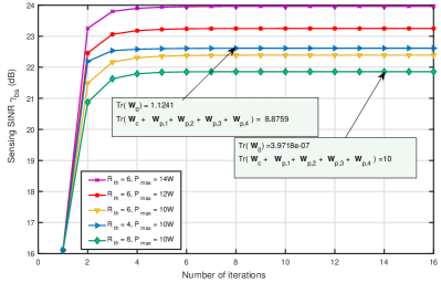
Fig. 4 compares the attained sensing SINR against the transmit power of our proposed design with other benchmark schemes, i.e., the STAR-RIS aided network with RSMA scheme without sensing signals, the STAR-RIS aided network involving NOMA/SDMA scheme, and the traditional/Random/Non RIS aided network with RSMA scheme. It is observable that as transmit power increases, there is a notable enhancement in the attained sensing SINR across all system designs. Besides, the STAR-RIS: RSMA and STAR-RIS: RSMA-N-sensing schemes yield the same $\gamma_{bs}$, which is consistent with the conclusion of Theorem 1. Furthermore, it is demonstrated that irrespective of the energy consumption of STAR-RIS and traditional RISs, the proposed STAR-RIS integrated with the RSMA approach consumes less power than those of all other benchmarks while achieving the same sensing SINR. The reasons may be explained as follows. Firstly, with the RSMA-based scheme, the inter-user interference can be effectively mitigated compared with the NOMA-based scheme and SDMA-based scheme, making it easier to meet GTs’ communication rate requirements. In this case, the signal power allocated for sensing is stronger, resulting in higher sensing SINR performance gain. Secondly, the STAR-RIS exhibits a remarkable capability to reshape beam propagation through the dynamic optimization of both transmission and reflection beamforming, ultimately leading to an enhancement in sensing SINR compared to traditional RISs. However, only reflection or transmission phases of the traditional RIS elements are optimized, which leads to limited performance gain. Thirdly, in contrast to the random STAR-RIS and Non-RIS schemes, our proposed scheme allows for more efficient signal propagation reconfiguration, thereby yielding a substantial performance enhancement. In summary, both the RSMA-based transmission strategy design and the dynamic optimization of STAR-RIS transmission and reflection beamforming have made tremendous contributions to the performance improvement of the ISAC system.

Refer to caption
Figure 4: Sensing SINR versus transmit power with different system designs.

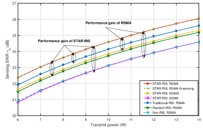
Fig. 5 presents the achieved maximal sensing SINR concerning the number of STAR-RIS elements $M$ across various system designs. It is observable that as the number of STAR-RIS elements increases, the system’s sensing performance progressively enhances. Similarly, the results indicate that the sensing SINR performance gain achieved through the combination of STAR-RIS and RSMA scheme surpasses that of other benchmarks, aligning with the conclusions in Fig. 4. The range of sensing performance gains that are fulfilled through the application of STAR-RIS and RSMA schemes are also illustrated in this figure. Notably, with an increase in the number of STAR-RIS elements, the performance gain gap between the STAR-RIS scheme and the Traditional RIS / Random RIS schemes progressively widens. The main factor driving this performance enhancement is that the STAR-RIS can manipulate both transmission and reflection beamforming simultaneously. Conversely, the sensing performance gains achieved by traditional RISs are hindered by their reliance on phase shift optimization alone. It is worth mentioning that in the Random RIS scheme, the TCs and RCs of STAR-RIS are generated randomly. In some cases, the randomly generated TCs and RCs may align closely with the sensing channel ${\bf h}_{t}$, which can positively impact system performance. However, due to the randomness of parameter generation and the alignments, there exists a certain degree of performance fluctuation. In addition, When the ISAC network transmits only communication waveforms, it achieves the same sensing SINR as when transmitting a combination of communication and dedicated sensing waveforms. This observation confirms the conclusions stated in Theorem 1.

Refer to caption
Figure 5: Sensing SINR versus the number of STAR-RIS elements $M$ with different system designs.

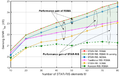
Fig. 6 characterizes the relationship between the optimized sensing SINR and communication rate threshold $R_{\rm th}$ with various system designs. One can see that as the rate threshold rises, the sensing SINR attained by all system designs experiences a decline. Intuitively, as the rate threshold gradually increases, a greater amount of energy at the BS is utilized to meet the heightened communication demands, ultimately leading to a deterioration in the achievable sensing SINR. Besides, the integration of STAR-RIS into networks results in a remarkable enhancement in sensing SINR, surpassing that achieved by other schemes. Consistent with the finding presented in Theorem 1 and results in Fig. 4, irrespective of $R_{\rm th}$, the ISAC network consistently maintains the same sensing SINR, whether or not dedicated sensing signals are incorporated.

Refer to caption
Figure 6: Relationship between sensing SINR and rate threshold across various system designs.

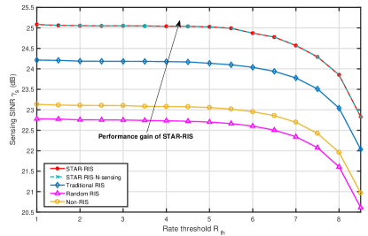
Fig. 7 provides the common rates and private rates of four GTs, and the corresponding private power allocation of GTs. It shows that the optimized results of private rates are consistent with the corresponding optimized power allocation. In other words, when the allocated common stream can meet the rate requirement of the GT, no private information stream will be allocated to it, and the corresponding private rate is 0. Furthermore, when the rate requirement of each GT is more stringent, a greater amount of power will be assigned to the private information stream to fulfill the rate requirement, thereby leading to the private rates of all GTs increasing.

Refer to caption
Figure 7: Optimized common rates, private rates and private power of each GT.

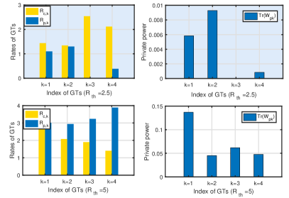
Fig. 8 depicts the common rates and private rates of four GTs versus various rate thresholds. It indicates that with an increase in the rate threshold, the proportion of private rate for each GT within the total rate also rises. However, the variation in common rates for each GT is not particularly evident as the rate threshold increases. The reason could be that, at a relatively low rate threshold, each GT exhibits a higher tolerance for inter-interference, and the communication rate requirements of each GT can be relatively easily satisfied through the utilization of the common information flow. Nonetheless, when the communication rate threshold is high, despite the capability to attain flexible interference management by dividing user messages into common and corresponding private messages, the effect of allocating common information on interference suppression and rate enhancement is limited. On the other words, after mitigating interference to a certain extent by leveraging the common information flow, it becomes crucial to increase private rates to satisfy the specific rate requirements of each GT.

Refer to caption
Figure 8: Common rates and private rates of GTs versus the rate thresholds.

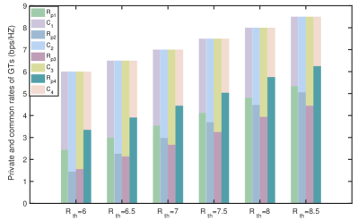
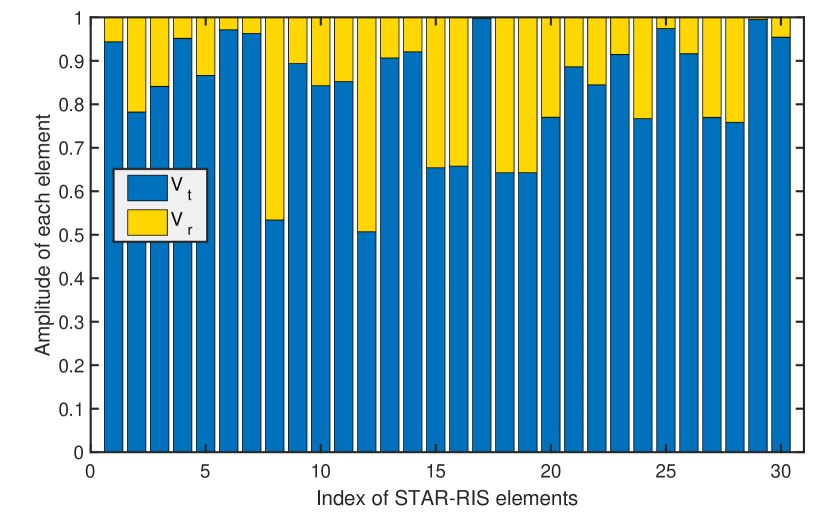
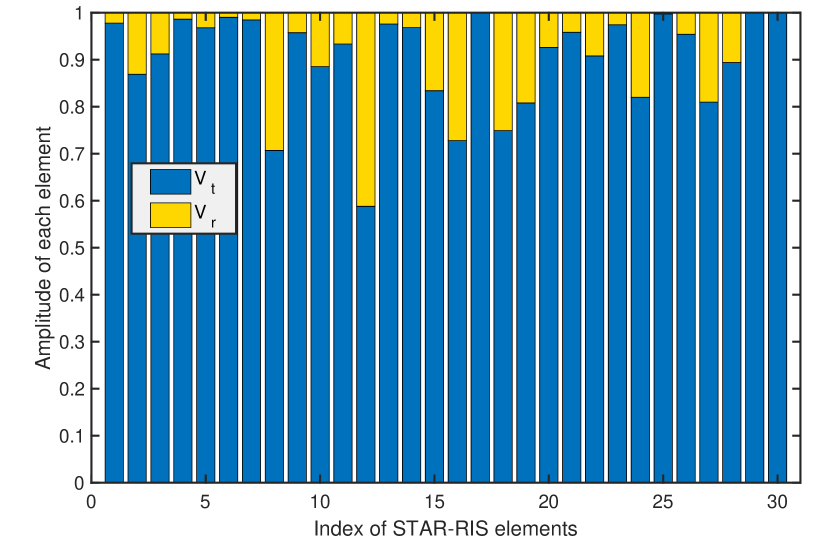
Fig. 9 provides the optimized amplitudes for transmission and reflection of every STAR-RIS element across various rate thresholds $R_{\rm th}$. It demonstrates that every element possesses the capability to adaptively manipulate the incoming signals based on the corresponding channel condition. In addition, the transmission amplitude coefficients are relatively larger than the reflection amplitude coefficients, which means that more energy is shared for enhancing the sensing performance. Besides, comparing the optimized results shown in Fig. 9(a) with that in Fig. 9(b), it is noticed that the reflection amplitude coefficients of each STAR-RIS element tend to be relatively greater when the rate threshold $R_{\rm th}$ is high. The reason is that when the rate requirements of GTs are large, the BS has to distribute a greater amount of energy into reflection space, so as to achieve signal enhancement for each GT.

Refer to caption
(a) $R_{\rm th}$ = 6
Refer to caption
(b) $R_{\rm th}$ = 1
Figure 9: Optimized amplitudes for every STAR-RIS element across different rate threshold.

V Conclusion

In this paper, we have explored the integration of STAR-RIS into an ISAC system employing the RSMA-based approach, where the maximization of sensing SINR was attained through the unified design of rate splitting in conjunction with precise adjustments of beamforming at BS and STAR-RIS, respectively. To address the formulated non-convex problem, the SCA-based iterative algorithm incorporating SDR, MM, and SROCR techniques has been devised. Simulation results manifest that, in comparison to other benchmark schemes, the employment of the RSMA scheme in conjunction with the transmission and reflection beamforming design at the STAR-RIS is crucial for enhancing the system’s sensing performance. Additionally, there is a balance to be established between achieving high-sensing SINR and maintaining reliable communication performance. For the considered ISAC network with a single target, the achievable sensing SINR is the same regardless of whether specially designed sensing signals are incorporated or not. For the mobile scenario involving multiple sensing targets and users in the STAR-RIS-enhanced ISAC system, we will investigate efficient sensing methods, specifically Time division (TD) sensing, signature sequence (SS) sensing, and hybrid TD-SS sensing.

Appendix A Proof of Theorem 1

According to the optimized solution $\{\widehat{{\bf W}}_{c},\widehat{{\bf W}}_{{\rm p},k},\widehat{{\bf W}}_{0}\}$ for sub-problem ${\mathbf{P}}_{\mathbf{B_{1}}}$, we can reconstruct one set of new solution $\{\overline{{\bf W}}_{c},\overline{{\bf W}}_{{\rm p},k},\overline{{\bf W}}_{0}\}$, which are mathematical modeled as

$\displaystyle\overline{{\bf W}}_{c}=\widehat{{\bf W}}_{c}+\zeta_{c}\widehat{{\bf W}}_{0},~{}\overline{{\bf W}}_{{\rm p},k}=\widehat{{\bf W}}_{{\rm p},k}+\zeta_{k}\widehat{{\bf W}}_{0},$ (41)
$\displaystyle\overline{{\bf W}}_{0}=0,~{}~{}\zeta_{c}+\sum\nolimits_{k=1}^{K}\zeta_{k}=1.$

By substituting the new set of solution into constraint (8b), we have

$\displaystyle R_{c,k}=\log_{2}\left(1+\frac{{\rm Tr}({\bf H}_{k}\overline{{\bf W}}_{c})}{\sum\nolimits_{i=1}^{K}{\rm Tr}({\bf H}_{k}\overline{{\bf W}}_{{\rm p},i})+\sigma_{k}^{2}}\right)$
$\displaystyle=\log_{2}\left(\tfrac{{\rm Tr}({\bf H}_{k}(\widehat{{\bf W}}_{c}+\zeta_{c}\widehat{{\bf W}}_{0}+\sum\limits_{i=1}^{K}(\widehat{{\bf W}}_{{\rm p},i}+\zeta_{i}\widehat{{\bf W}}_{0})))+\sigma_{k}^{2}}{\sum\nolimits_{i=1}^{K}{\rm Tr}({\bf H}_{k}(\widehat{{\bf W}}_{{\rm p},i}+\zeta_{i}\widehat{{\bf W}}_{0}))+\sigma_{k}^{2}}\right)$
$\displaystyle=\log_{2}\left(\frac{{\rm Tr}({\bf H}_{k}(\widehat{{\bf W}}_{c}+\sum\limits_{i=1}^{K}\widehat{{\bf W}}_{{\rm p},i}+\widehat{{\bf W}}_{0}))+\sigma_{k}^{2}}{\sum\nolimits_{i=1}^{K}{\rm Tr}({\bf H}_{k}(\widehat{{\bf W}}_{{\rm p},i}+\zeta_{i}\widehat{{\bf W}}_{0}))+\sigma_{k}^{2}}\right)$
$\displaystyle\overset{(a)}{\geq}\log_{2}\left(\frac{{\rm Tr}({\bf H}_{k}(\widehat{{\bf W}}_{c}+\sum\limits_{i=1}^{K}\widehat{{\bf W}}_{{\rm p},i}+\widehat{{\bf W}}_{0}))+\sigma_{k}^{2}}{\sum\nolimits_{i=1}^{K}{\rm Tr}({\bf H}_{k}(\widehat{{\bf W}}_{{\rm p},i}+\widehat{{\bf W}}_{0}))+\sigma_{k}^{2}}\right)$
$\displaystyle=\log_{2}\left(1+\frac{{\rm Tr}({\bf H}_{k}\widehat{{\bf W}}_{c})}{\sum\nolimits_{i=1}^{K}{\rm Tr}({\bf H}_{k}(\widehat{{\bf W}}_{{\rm p},i}+\widehat{{\bf W}}_{0}))+\sigma_{k}^{2}}\right)$
$\displaystyle\overset{(b)}{\geq}\sum\nolimits_{k=1}^{K}c_{k}.$

The step $(a)$ holds due to the fact that $\sum\nolimits_{i=1}^{K}\zeta_{i}\leq 1$, and step $(b)$ holds since $\{\widehat{{\bf W}}_{c},\widehat{{\bf W}}_{{\rm p},k},\widehat{{\bf W}}_{0}\}$ is one set of feasible solutions for ${\mathbf{P}}_{\textbf{B1-1}}$. On the other hand, by substituting the new set of solutions into constraint (8c), we have

$\displaystyle R_{{\rm p},k}=\log_{2}\left(1+\frac{{\rm Tr}({\bf H}_{k}\overline{{\bf W}}_{{\rm p},k})}{\sum\nolimits_{j\neq k}^{K}{\rm Tr}({\bf H}_{k}\overline{{\bf W}}_{{\rm p},j})+\sigma_{k}^{2}}\right)$
$\displaystyle=\log_{2}\left(\frac{{\rm Tr}({\bf H}_{k}(\sum\nolimits_{i=1}^{K}\widehat{{\bf W}}_{{\rm p},i}+\widehat{{\bf W}}_{0}))}{\sum\nolimits_{j\neq k}^{K}{\rm Tr}({\bf H}_{k}(\widehat{{\bf W}}_{{\rm p},j}+\zeta_{j}\widehat{{\bf W}}_{0}))+\sigma_{k}^{2}}\right)$
$\displaystyle\overset{(c)}{\geq}\log_{2}\left(\frac{{\rm Tr}({\bf H}_{k}(\sum\nolimits_{i=1}^{K}\widehat{{\bf W}}_{{\rm p},i}+\widehat{{\bf W}}_{0}))}{\sum\nolimits_{j\neq k}^{K}{\rm Tr}({\bf H}_{k}(\widehat{{\bf W}}_{{\rm p},j}+\widehat{{\bf W}}_{0}))+\sigma_{k}^{2}}\right)$
$\displaystyle=\log_{2}\left(1+\frac{{\rm Tr}({\bf H}_{k}\widehat{{\bf W}}_{{\rm p},k})}{\sum\nolimits_{j\neq k}^{K}{\rm Tr}({\bf H}_{k}(\widehat{{\bf W}}_{{\rm p},j}+\widehat{{\bf W}}_{0}))+\sigma_{k}^{2}}\right)$
$\displaystyle\overset{(d)}{\geq}R_{k}^{\rm th}-c_{k}.$

The validity of step $(c)$ is attributed to the fact that $\sum\nolimits_{j\neq k}^{K}\zeta_{j}\leq 1$, and step $(d)$ holds since $\{\widehat{{\bf W}}_{c},\widehat{{\bf W}}_{{\rm p},k},\widehat{{\bf W}}_{0}\}$ is one set of feasible solutions for ${\mathbf{P}}_{\textbf{B1-1}}$. Therefore, $\{\overline{{\bf W}}_{c},\overline{{\bf W}}_{{\rm p},k},\overline{{\bf W}}_{0}\}$ is also one set of feasible solutions for ${\mathbf{P}}_{\textbf{B1-1}}$. It can also achieve the optimal sensing SINR, which is not inferior to that achieved by $\{\widehat{{\bf W}}_{c},\widehat{{\bf W}}_{{\rm p},k},\widehat{{\bf W}}_{0}\}$. The proof for Theorem 1 is completed.

References

  • [1] C. Han, Y. Wu, Z. Chen, Y. Chen and G. Wang, “THz ISAC: a physical-layer perspective of terahertz integrated sensing and communication,” IEEE Commun. Mag., vol. 62, no. 2, pp. 102-108, Feb. 2024.
  • [2] R. Jiang, K. Xiong, H. -C. Yang, P. Fan, Z. Zhong and K. B. Letaief, “On the coverage of UAV-assisted SWIPT networks with nonlinear EH model,” IEEE Trans. Wirel. Commun., vol. 21, no. 6, pp. 4464-4481, June 2022.
  • [3] M. Liu et al., “A nonorthogonal uplink/downlink IoT solution for next-generation ISAC systems,” IEEE Internet of Things J., vol. 11, no. 5, pp. 8224-8239, Mar. 2024.
  • [4] X. Wang, Z. Fei and Q. Wu, “Integrated sensing and communication for RIS-assisted backscatter systems,” IEEE Internet of Things J., vol. 10, no. 15, pp. 13716-13726, Aug. 2023.
  • [5] Y. Cui, F. Liu, X. Jing and J. Mu, “Integrating sensing and communications for ubiquitous IoT: applications, trends, and challenges,” IEEE Network, vol. 35, no. 5, pp. 158-167, Sep. 2021.
  • [6] Z. Wei, F. Liu, C. Masouros, N. Su and A. P. Petropulu, “Toward multi-functional 6G wireless networks: integrating sensing, communication, and security,” IEEE Commun. Mag., vol. 60, no. 4, pp. 65-71, Apr. 2022.
  • [7] Z. Chen et al., “ISACoT: integrating sensing with data traffic for ubiquitous IoT devices,” IEEE Commun. Mag., vol. 61, no. 5, pp. 98-104, May 2023.
  • [8] J. Mu, R. Zhang, Y. Cui, N. Gao and X. Jing, “UAV meets integrated sensing and communication: challenges and future directions,” IEEE Commun. Mag., vol. 61, no. 5, pp. 62-67, May 2023.
  • [9] Z. Yang, M. Chen, W. Saad and M. Shikh-Bahaei, “Downlink sum-rate maximization for rate splitting multiple access (RSMA),” in proc. IEEE ICC, Dublin, Ireland, 2020, pp. 1-6.
  • [10] B. Rimoldi and R. Urbanke, “A rate-splitting approach to the Gaussian multiple-access channel,” IEEE Trans. Inf. Theory, vol. 42, no. 2, pp. 364-375, Mar. 1996.
  • [11] Q. Zhang, L. Zhu, Y. Chen and S. Jiang, “Energy-efficient traffic offloading for RSMA-based hybrid satellite terrestrial networks with deep reinforcement learning,” China Commun., vol. 21, no. 2, pp. 49-58, Feb. 2024.
  • [12] M. Can, M. C. Ilter and I. Altunbas, “Data-oriented downlink RSMA systems,” IEEE Commun. Lett., vol. 27, no. 10, pp. 2812-2816, Oct. 2023.
  • [13] Y. Liu, K. Xiong, Y. Zhu, H. -C. Yang, P. Fan and K. B. Letaief, “Outage analysis of IRS-assisted UAV NOMA downlink wireless networks,” IEEE Internet of Things J., vol. 11, no. 6, pp. 9298-9311, Mar. 2024.
  • [14] J. Sang et al., “Coverage enhancement by deploying RIS in 5G commercial mobile networks: field trials,” IEEE Wirel. Commun., vol. 31, no. 1, pp. 172-180, Feb. 2024.
  • [15] W. Khalid, Z. Kaleem, R. Ullah, T. Van Chien, S. Noh and H. Yu, “Simultaneous transmitting and reflecting-reconfigurable intelligent surface in 6G: design guidelines and future perspectives,” IEEE Network, vol. 37, no. 5, pp. 173-181, Sept. 2023.
  • [16] K. Xie, G. Cai, G. Kaddoum and J. He, “Performance analysis and resource allocation of STAR-RIS-aided wireless-powered NOMA system,” IEEE Trans. Commun., vol. 71, no. 10, pp. 5740-5755, Oct. 2023.
  • [17] W. Khalid, Z. Kaleem, R. Ullah, T. Van Chien, S. Noh and H. Yu, “Simultaneous transmitting and reflecting-reconfigurable intelligent surface in 6G: design guidelines and future perspectives,” IEEE Network, vol. 37, no. 5, pp. 173-181, Sept. 2023.
  • [18] K. Zhong, J. Hu, C. Pan, M. Deng and J. Fang, “Joint waveform and beamforming design for RIS-aided ISAC systems,” IEEE Signal Process. Lett., vol. 30, pp. 165-169, 2023.
  • [19] M. Luan, B. Wang, Z. Chang, T. H$\ddot{a}$m$\ddot{a}$l$\ddot{a}$inen and F. Hu, “Robust beamforming design for RIS-aided integrated sensing and communication system,” IEEE Trans. Intell. Transp. Syst., vol. 24, no. 6, pp. 6227-6243, June 2023.
  • [20] Y. Eghbali, S. Faramarzi, S. K. Taskou, M. R. Mili, M. Rasti and E. Hossain, “Beamforming for STAR-RIS-aided integrated sensing and communication using meta DRL,” early access in IEEE Wirel. Commun. Lett., 2024.
  • [21] Z. Liu, X. Li, H. Ji, H. Zhang and V. C. M. Leung, “Toward STAR-RIS-empowered integrated sensing and communications: joint active and passive beamforming design,” IEEE Trans. Veh. Technol, vol. 72, no. 12, pp. 15991-16005, Dec. 2023.
  • [22] P. Saikia, A. Jee, K. Singh, C. Pan, T. A. Tsiftsis and W. -J. Huang, “RIS-aided integrated sensing and communications,” in Proc. IEEE GLOBECOM, Kuala Lumpur, Malaysia, 2023, pp. 5080-5085.
  • [23] P. Gao, L. Lian and J. Yu, “Cooperative ISAC with direct localization and rate-splitting multiple access communication: a pareto optimization framework,” IEEE J. Sel. Areas Commun., vol. 41, no. 5, pp. 1496-1515, May 2023.
  • [24] C. Hu, Y. Fang and L. Qiu, “Joint transmit and receive beamforming design for uplink RSMA enabled integrated sensing and communication systems,” in Proc. IEEE WCNC Glasgow, United Kingdom, 2023, pp. 1-6.
  • [25] C. Xu, B. Clerckx, S. Chen, Y. Mao and J. Zhang, “Rate-splitting multiple access for multi-antenna joint radar and communications,” IEEE Journal of Selected Topics in Signal Processing, vol. 15, no. 6, pp. 1332-1347, Nov. 2021.
  • [26] Z. Liu, Y. Jint, B. Cao and R. Lu, “RISAC: rate-splitting multiple access enabled integrated sensing and communication systems,” in Proc. IEEE ICC 2023, Rome, Italy, 2023, pp. 6449-6454.
  • [27] Z. Chen, J. Wang, Z. Tian, M. Wang, Y. Jia and T. Q. S. Quek, “Joint rate splitting and beamforming design for RSMA-RIS-assisted ISAC system,” IEEE Wirel. Commun. Lett., vol. 13, no. 1, pp. 173-177, Jan. 2024.
  • [28] R. Zhang, K. Xiong, Y. Lu, P. Fan, D. W. K. Ng and K. B. Letaief, “Energy efficiency maximization in RIS-assisted SWIPT networks with RSMA: a PPO-Based Approach,” IEEE J. Sel. Areas Commun., vol. 41, no. 5, pp. 1413-1430, May 2023.
  • [29] Z. He, W. Xu, H. Shen, D. W. K. Ng, Y. C. Eldar and X. You, “Full-duplex communication for ISAC: joint beamforming and power optimization,” IEEE J. Sel. Areas Commun., vol. 41, no. 9, pp. 2920-2936, Sept. 2023.
  • [30] M. Jiang, Y. Li, Q. Zhang and J. Qin, “Joint position and time allocation optimization of UAV enabled time allocation optimization networks,” IEEE Trans. Commun., vol. 67, no. 5, pp. 3806-3816, May 2019.
  • [31] P. Cao, J. Thompson and H. V. Poor, “A sequential constraint relaxation algorithm for rank-one constrained problems,” in Proc. 2017 25th European Signal Processing Conference (EUSIPCO), Kos, Greece, 2017, pp. 1060-1064.
  • [32] K. Y. Wang, A. M. So, T. H. Chang, W. K. Ma, C. Y. Chi, “Outage constrained robust transmit optimization for multiuser MISO downlinks: tractable approximations by conic optimization,” IEEE Trans. Signal Process., vol. 62, no. 21, pp. 5690-5705, Nov. 2014.
  • [33] Y. Liu, K. Xiong, Q. Ni, P. Fan and K. B. Letaief, “UAV-assisted wireless powered cooperative mobile edge computing: joint offloading, CPU control, and trajectory optimization,” IEEE Internet of Things J., vol. 7, no. 4, pp. 2777-2790, April 2020.
  • [34] N. Xue, X. Mu, Y. Liu and Y. Chen, “NOMA assisted full space STAR-RIS-ISAC,” early access in IEEE Trans. Wirel. Commun., 2024.