Post-Newtonian templates for phase evolution of spherical extreme mass ratio inspirals

Abstract

We present various post-Newtonian (PN) models for the phase evolution of compact objects moving along quasi-spherical orbits in Kerr spacetime derived by using the 12PN analytic formulas of the energy, angular momentum and their averaged rates of change calculated in the framework of the black hole perturbation theory. To examine the convergence of time-domain PN models (TaylorT families), we evaluate the dephasing between approximants with different PN orders. We found that the TaylorT1 model shows the best performance and the performance of the TaylorT2 is the next best. To evaluate the convergence of frequency-domain PN models (TaylorF families), we evaluate the mismatch between approximants with different orders. We found that the performance of the TaylorF2 model is comparable with the TaylorT2 model. Although the TaylorT2 and TaylorF2 models are not so accurate as the TaylorT1, the fully analytical expressions give us easy-to-handle templates and are useful to discuss effects beyond general relativity.

I Introduction

Extreme mass ratio inspirals (EMRIs) are important targets of space-borne gravitational wave (GW) detectors, like Laser Interferometer Space Antenna (LISA) [1], TianQin [2], and Taiji [3]. An EMRI consists of a compact object orbiting and plunging into a massive black hole, which is expected to exist in the center of galactic nuclei. Before plunging into the central black hole, the object emits GWs including a huge number of cycles. The observation and data analysis of the GWs allow us to measure the intrinsic parameters of the EMRI system precisely and will provide insights into the theory of gravity, the physics and astrophysics of black holes [4, 5, 6].

Matched filtering is one of promising techniques to analyze the observed GWs and extract the physical information from signals emitted by EMRIs accurately and efficiently. This technique requires waveform templates representing the real signals from EMRIs accurately. The GW templates of EMRIs are often calculated by black hole perturbation theory because the extreme mass ratio is suitable for the small parameter in the perturbative expansion.

In the context of black hole perturbation theory, an EMRI is modeled as a point mass moving in Kerr spacetime, and the GWs are represented by the gravitational perturbations induced by the point mass. The gravitational perturbations of Kerr black hole are described by the perturbations of the Newman-Penrose variables [7], which satisfy the Teukolsky equations [8, 9] with the source constructed from the energy-momentum tensor for the point mass. This means that we need to know the precise motion of the point mass to calculate the GWs accurately by solving the Teukolsky equation.

In the test-mass limit, the motion is expressed by a geodesic in Kerr spacetime. Taking into account the self-interaction with the own gravitational field, however, a deviation of the mass’ motion from the geodesic arises. This can be interpreted as the “self-force” (see Refs. [10, 11] and the references therein) effect. The dominant contribution of the gravitational self-force to the mass’ motion is the time-averaged dissipative piece at the first order of the mass ratio, which induces the losses of the energy and angular momentum of the point mass and drives the gradual inspiral into the central black hole. The dissipative effect is most noticeable on the orbital phase and therefore the GW phase. A phase difference of $O(1)$ significantly reduces the overlap between an observed signal and the corresponding template, and leads to failure of the detection or the accurate estimation of the physical parameters. Therefore, it is important to calculate the time-averaged dissipative self-force at high precision.

The time-averaged dissipative self-force can be rewritten in the secular changes of three orbital parameters, the energy, azimuthal angular momentum, and Carter parameter of the point mass. There are several works on calculating the rates of the secular change in both numerical and analytical approaches based on the black hole perturbation theory. The state-of-the-art studies on the numerical approach can provide the data of the secular evolution for general bound orbits in Kerr spacetime [12, 13, 14, 15]. Since the numerical calculation costs a lot of computational resources, however, the use of combination with the analytical approach is expected to reduce the cost and improve the efficiency. There have been several efforts in analytically calculating the secular evolution of the orbital parameters since the 1990s (see Ref. [16, 17] and the references therein). The post-Newtonian (PN) formulas of the secular evolution for general bound orbits are presented in our previous works [18, 19, 20]. The recent advances in computers have made it possible to extend the analytical calculation to the higher PN order. Several works on calculating the higher PN corrections have been done in Refs. [21, 22, 23, 24, 25].

In this work, we focus on the secular evolution of orbits off equatorial plane in Kerr spacetime, which has attracted less attention in the study of the analytic calculation of the self-force so far. As the first step, we consider the evolution of a spherical orbit, which is an orbit with a constant radius on a plane precessing around the rotation axis of the central black hole. We calculate the 12PN formulas for the secular change of orbital parameters for spherical orbits with arbitrary inclination angle, through the procedure based on the adiabatic approximation proposed in Refs. [19, 20] .

To study the convergence of the PN formulas and the impact of the higher corrections on the accuracy of the gravitational waveform, we derive the PN templates of the phase evolution, the time-domain, TaylorT and frequency-domain, TaylorF models [27, 28], for quasi-spherical orbits. Although the TaylorT and TaylorF templates in the context of the black hole perturbation theory have been derived in Ref. [29], the work is restricted to the circular orbit case in Schwarzschild spacetime in exchange for the remarkably high, 22PN order. This work presents the extension into the spherical orbit case in Kerr spacetime, and we investigate how the convergence of the PN formulas is influenced by the orbital inclination and the spin of the central black hole.

This paper is organized as follows. In Sec. II, we briefly review the spherical orbit in Kerr spacetime and its secular evolution driven by the dissipation due to the gravitational radiation. In Sec. III, we present the TaylorT and TaylorF models derived in a similar manner to Ref. [29]. In addition, we propose alternative choices of the TaylorT1 and TaylorT4 templates, which appear because of increasing the number of orbital parameters. In Sec. IV, we examine the performance of the Taylor models for several sets of the orbital inclination and the black hole spin. In Sec. V, we summarize our results. In Appendices A–I, we present the explicit expressions of the PN coefficients of the orbital energy and angular momentum, their time averaged rates of change, the TaylorT and TaylorF templates, up to the 4.5PN order. Throughout this paper, we adopt the geometrized units with $c=G=1$ and metric signature $(-+++)$, and the Kerr metric is described in the Boyer–Lindquist coordinates $(t,r,\theta,\varphi)$.

II Adiabatic evolution of bound orbits in Kerr spacetime

In this section, we briefly review the generic bound geodesics in Kerr spacetime and the formulation of the adiabatic evolution with the secular change of the orbital parameters characterizing the geodesics. We also present the formulation reduced to the spherical orbit case which we consider in this paper.

II.1 Geodesic equations in Kerr spacetime

The equations of motion for generic orbits in Kerr spacetime with mass $M$ and Kerr parameter $a$ are

$$\left(\frac{dr}{d\lambda}\right)^{2} = V_{r}(r),\quad\left(\frac{d\cos\theta}{d\lambda}\right)^{2}=V_{\theta}(\cos\theta),$$ (1)

$$\frac{dt}{d\lambda} = V_{tr}(r)+V_{t\theta}(\cos\theta),$$ (2)

$$\frac{d\varphi}{d\lambda} = V_{\varphi r}(r)+V_{\varphi\theta}(\cos\theta),$$ (3)

where $\lambda$ is defined by $d/d\lambda=\Sigma d/d\tau$ ($\Sigma\equiv r^{2}+a^{2}\cos^{2}\theta$), and

$$V_{r}(r) \equiv \left[P(r)\right]^{2}-\Delta\left[r^{2}+(aE-L)^{2}+C\right],$$ (4)

$$P(r) \equiv E(r^{2}+a^{2})-aL,\quad\Delta\equiv r^{2}-2Mr+a^{2},$$ (5)

$$V_{\theta}(z) \equiv C-\left[C+a^{2}(1-E^{2})+L^{2}\right]z^{2}+a^{2}(1-E^{2})z^{4},$$ (6)

$$V_{tr}(r) \equiv \frac{r^{2}+a^{2}}{\Delta}P(r),\quad V_{t\theta}(z)\equiv-a(aE-L-aEz^{2}),$$ (7)

$$V_{\varphi r}(r) \equiv \frac{aP(r)}{\Delta},\quad V_{\varphi\theta}(z)\equiv-aE+\frac{L}{1-z^{2}}.$$ (8)

Here, $z=\cos\theta$. The geodesic motion is characterized by three parameters, $I^{A}=\{E,L,C\}$, corresponding to the specific energy, angular momentum and Carter constant, respectively. For bound orbits, we can choose an alternative parametrization analogous to celestial mechanics, $\iota^{A}=\{p,e,\chi\}$, defined by

$$p\equiv\frac{2r_{a}r_{p}}{M(r_{a}+r_{p})},\quad e\equiv\frac{r_{a}-r_{p}}{r_{a}+r_{p}},\quad\cos\chi\equiv\frac{L}{\sqrt{L^{2}+C}},$$ (9)

where $r_{p}$ and $r_{a}$ are the values of $r$ at the periapsis and apoapsis. We refer $p$, $e$, and $\chi$ to the non-dimensional semi-latus rectum, eccentricity, and inclination angle, respectively.

For bound orbits, the radial and polar motions are periodic with respect to $\lambda$. The radial and polar periods are given by

$$\Lambda_{r}=2\int_{r_{p}}^{r_{a}}\frac{dr}{\sqrt{V_{r}(r)}},\quad\Lambda_{\theta}=4\int_{0}^{z_{\textrm{min}}}\frac{dz}{\sqrt{V_{\theta}(z)}},$$ (10)

where $z_{\textrm{min}}=\cos\theta_{\textrm{min}}$, $\theta_{\textrm{min}}$ is the minimal value of $\theta$. The radial and polar frequencies with respect to $\lambda$ are given by the periods as

$$\Omega_{r}\equiv\frac{2\pi}{\Lambda_{r}},\quad\Omega_{\theta}\equiv\frac{2\pi}{\Lambda_{\theta}}.$$ (11)

The temporal and azimuthal frequencies with respect to $\lambda$ can be derived as the time average along the orbit:

$$\Omega_{t} \equiv \lim_{T\to\infty}\frac{1}{2T}\int_{-T}^{T}\frac{dt}{d\lambda}d\lambda=\frac{1}{\Lambda_{r}}\int_{0}^{\Lambda_{r}}V_{tr}(r(\lambda))d\lambda+\frac{1}{\Lambda_{\theta}}\int_{0}^{\Lambda_{\theta}}V_{t\theta}(\cos\theta(\lambda))d\lambda,$$ (12)

$$\Omega_{\varphi} \equiv \lim_{T\to\infty}\frac{1}{2T}\int_{-T}^{T}\frac{d\varphi}{d\lambda}d\lambda=\frac{1}{\Lambda_{r}}\int_{0}^{\Lambda_{r}}V_{\varphi r}(r(\lambda))d\lambda+\frac{1}{\Lambda_{\theta}}\int_{0}^{\Lambda_{\theta}}V_{\varphi\theta}(\cos\theta(\lambda))d\lambda.$$ (13)

The fundamental frequencies with respect to the time coordinate for bound geodesics in Kerr spacetime are given by

$$\omega_{J}(E,L,C)=\frac{\Omega_{J}(E,L,C)}{\Omega_{t}(E,L,C)},$$ (14)

where $J=\{r,\theta,\varphi\}$.

The adiabatic evolution of $\iota^{A}$ and orbital phase (i.e., rotational angle) $\Phi$ are described by

$$\dot{\iota}^{A} = (G^{-1})^{A}_{B}\dot{I}^{B},$$ (15)

$$\dot{\Phi} = \omega_{\varphi},$$ (16)

where a dot ($\cdot$) over variable denotes derivative with respect to $t$ and $G^{A}_{B}\equiv(\partial I^{A}/\partial\iota^{B})$ is the Jacobian for the transformation from $\iota^{A}$ to $I^{A}$.

II.2 Spherical orbits

A spherical orbit is an bound orbit with $e=0$ (or equivalently, $r_{p}=r_{a}$), and hence is characterized by two orbital parameters, $\{p,\chi\}$. The parameters, $\{E,L,C\}$, are not independent for spherical orbits. In this work, we choose $\{E,L\}$ from them as a set of independent parameters.

For the later convenience, we introduce $x\equiv(M\omega_{\varphi})^{1/3}$ and $Y\equiv\cos\chi$ instead of $p$ and $\chi$ respectively. Since $x$ corresponds to the characteristic velocity in the motion, it is used as the parameter of the PN expansion. By using the set of $\{x,Y\}$, the equations of orbital evolution, Eqs. (15) and (16), for spherical orbits, are reexpressed as

$$\dot{x} = (G^{-1})^{x}_{E}\dot{E}+(G^{-1})^{x}_{L}\dot{L},$$ (17)

$$\dot{Y} = (G^{-1})^{Y}_{E}\dot{E}+(G^{-1})^{Y}_{L}\dot{L},$$ (18)

$$\dot{\Phi} = \frac{x^{3}}{M},$$ (19)

where $G^{A}_{B}\equiv\partial(E,L)/\partial(x,Y)$ is the Jacobian for the transformation from $\{x,Y\}$ to $\{E,L\}$.

The specific energy and angular momentum for a spherical orbit at the leading order of the mass ratio are given in the form of the PN expansion as

$$E^{(n)}(x,Y) = 1-\frac{1}{2}x^{2}\sum_{k=0}^{n}\tilde{E}_{k}x^{k},$$ (20)

$$L^{(n)}(x,Y) = \frac{Y}{x}\sum_{k=0}^{n}\tilde{L}_{k}x^{k}.$$ (21)

The superscript $(n)$ in the left hand side of the above equations means that the formula includes the terms up to $n$-th order terms of $x$ relative to the Newtonian order . For example, the 2.5PN ($n=5$) energy and angular momentum are

$$E^{(5)}(x,Y) = 1-\frac{1}{2}x^{2}\left\{1-\frac{3}{4}x^{2}-\left(\frac{4}{3}-4Y\right)qx^{3}-\left[\frac{27}{8}-\left(\frac{1}{2}+Y-\frac{5}{2}Y^{2}\right)q^{2}\right]x^{4}+(2+6Y)qx^{5}\right\},$$

$$L^{(5)}(x,Y) = \frac{Y}{x}\left\{1+\frac{3}{2}x^{2}+\left(\frac{2}{3}-4Y\right)x^{3}+\left[\frac{27}{8}-\left(\frac{1}{4}+\frac{Y}{2}-\frac{7}{4}Y^{2}\right)q^{2}\right]x^{4}-(1+6Y)x^{5}\right\},$$

where $q=a/M$. In Appendix A, we show the expansion coefficients, $\tilde{E}_{k}$ and $\tilde{L}_{k}$, for $k\leq 9$ explicitly (the higher order terms are publicly available online [31]).

The averaged rates of change of $E$ and $L$ at the linear order of the mass ratio are given by the black hole perturbation technique [19, 20] as

$$\dot{E}^{(n)}(x,Y) = -\frac{32}{5}\frac{\mu}{M^{2}}x^{10}\sum_{k=0}^{n}\tilde{\dot{E}}_{k}x^{k},$$ (22)

$$\dot{L}^{(n)}(x,Y) = -\frac{32}{5}\frac{\mu}{M}x^{7}\sum_{k=0}^{n}\tilde{\dot{L}}_{k}x^{k},$$ (23)

where $\mu$ denotes the mass of a point mass. In the same way of Eqs. (20) and (21), the superscript $(n)$ means the truncation order. It should be noted that the coefficients, $\tilde{\dot{E}}_{k}$ and $\tilde{\dot{L}}_{k}$, include some terms with the power of $\ln x$ for $k\geq 6$. In Appendix B, we show $\tilde{\dot{E}}_{k}$ and $\tilde{\dot{L}}_{k}$ for $k\leq 9$ explicitly.

III Post-Newtonian templates of the phase evolution

The PN approximation provides various expressions of the phase evolution with different variables and functional forms while keeping the same PN order [27, 28, 29]. In this section, we present several PN families of the phase evolution of quasi-spherical orbits, TaylorT1, TaylorT2, TaylorT3, and TaylorT4 in the time domain , and TaylorF1, TaylorF2 in the frequency domain, in a similar manner to Refs. [27, 28, 29]. In addition, we present subfamilies of TaylorT1 and TaylorT4, which appear because the number of the orbital parameters increases compared to circular orbits.

III.1 TaylorT1

Substituting the PN formulas given by Eqs. (20)–(23) to $E$, $L$, $\dot{E}$ and $\dot{L}$ in the right hand sides of Eqs. (17) and (18), we obtain

$$\dot{x} = (G_{n}^{-1})^{x}_{E}\dot{E}^{(n)}+(G_{n}^{-1})^{x}_{L}\dot{L}^{(n)},$$ (24)

$$\dot{Y} = (G_{n}^{-1})^{Y}_{E}\dot{E}^{(n)}+(G_{n}^{-1})^{Y}_{L}\dot{L}^{(n)},$$ (25)

$$\dot{\Phi}_{\textrm{T1}}^{(n)} = \frac{x^{3}}{M},$$ (26)

where $(G_{n})^{A}_{B}=\partial(E^{(n)},L^{(n)})/\partial(x,Y)$. Note that we do not perform any expansion with respect to $x$ after the substitution. Therefore, the right hand sides of Eqs. (24) and (25) can be expressed by rational functions of $x$, $\ln x$ and $Y$ although we do not show them explicitly because of their complexity.

By analogy of the circular orbit case, we refer the numerical solution of Eqs. (24)–(26) as the TaylorT1 approximant.

III.2 TaylorT4

Expanding the right hand sides of Eqs. (24) and (25) with respect to $x$, we obtain

$$\dot{x} = \frac{32}{5}\frac{\mu}{M^{2}}x^{9}\sum_{k=0}^{n}\tilde{\dot{x}}_{k}x^{k}$$ (27)

$$= \frac{32}{5}\frac{\mu}{M^{2}}x^{9}\left[1-\frac{743}{336}x^{2}+\left(4\pi-\frac{73Y+40}{12}q\right)x^{3}+\cdots+\left(\mbox{truncated at}\ O(x^{n+1})\right)\right],$$ (28)

$$\dot{Y} = -\frac{244}{15}\frac{\mu}{M^{2}}x^{8}q(1-Y^{2})\sum_{k=0}^{n}\tilde{\dot{Y}}_{k}x^{k}$$ (29)

$$= -\frac{244}{15}\frac{\mu}{M^{2}}x^{8}q(1-Y^{2})\left[x^{3}-\frac{13}{244}qYx^{4}-\frac{10461}{1708}x^{5}+\cdots+\left(\mbox{truncated at}\ O(x^{n+1})\right)\right],$$ (30)

$$\dot{\Phi}_{\textrm{T4}}^{(n)} = \frac{x^{3}}{M}.$$ (31)

The expansion coefficients $\tilde{\dot{x}}_{k}$ and $\tilde{\dot{Y}}_{k}$ for $k\leq 9$ are given in Appendix C.

It should be noted that, since the PN formulas of the first and second terms in the right hand side of Eq. (25) are given as

$$(G_{n}^{-1})^{Y}_{E}\dot{E}^{(n)} = \frac{\mu}{M^{2}}\left[\frac{32}{5}Yx^{8}-\frac{3502}{105}Yx^{10}+\left(\frac{384\pi-512q}{15}Y+\frac{152}{3}qY^{2}\right)x^{11}+\cdots\right],$$

$$(G_{n}^{-1})^{Y}_{L}\dot{L}^{(n)} = \frac{\mu}{M^{2}}\left[-\frac{32}{5}Yx^{8}+\frac{3502}{105}Yx^{10}-\left(\frac{384\pi-512q}{15}Y+\frac{172}{5}qY^{2}+\frac{244}{15}q\right)x^{11}+\cdots\right],$$

the first two leading terms of them are canceled each other out. Hence, the leading term in the PN expansion of $\dot{Y}$ is considered as the 1.5PN contribution of the adiabatic evolution.

The TaylorT4 approximant is obtained by solving Eqs. (27)–(31) numerically.

III.3 TaylorT2

In the circular orbit case, the TaylorT2 approximant gives $t$ and $\Phi$ as functions of $x$ which is regarded as the parametric variable. To obtain a similar expression for the spherical orbit case, first we derive the equation of $Y(x)$ as

$$\frac{dY}{dx} = \frac{dY}{dt}\left(\frac{dx}{dt}\right)^{-1}$$ (32)

$$= -q(1-Y^{2})\left[\frac{61}{24}x^{2}-\frac{13}{96}qYx^{3}-\left(\frac{81217}{8064}+\frac{33+15Y^{2}}{128}q^{2}\right)x^{4}+\cdots\right].$$ (33)

We can transform Eq. (33) into the form of integral equation as

$$Y(x)=Y_{I}-\int_{x_{I}}^{x}dx^{\prime}q(1-Y^{2})\left[\frac{61}{24}x^{\prime 2}-\frac{13}{96}qYx^{\prime 3}-\left(\frac{81217}{8064}+\frac{33+15Y^{2}}{128}q^{2}\right)x^{\prime 4}+\cdots\right],$$ (34)

where $x_{I}$ is the value of $x$ at the initial time $t=0$ and $Y_{I}\equiv Y(x_{I})$. Considering that the integral term of Eq. (34) starts from $O(x^{3})$, we assume the PN formula of $Y(x)$ as

$$Y^{(n)}(x)=\tilde{Y}_{0}-q(1-\tilde{Y}_{0}^{2})\sum_{k=3}^{n}\tilde{Y}_{k}x^{k}.$$ (35)

Here the constant term, $\tilde{Y}_{0}$, is determined so that $Y^{(n)}(x_{I})=Y_{I}$. The superscript $(n)$ in the left hand side of the above expression again means the truncation order as explained below Eq. (21). Also, note that the coefficients $\tilde{Y}_{k}$ depend on $\ln x$ in general (later, we find that the dependence of $\ln x$ appears for $k\geq 9$). By substituting Eq. (35) to $Y$ in the integral equation (34) and comparing both sides by order of $x$, we find $\tilde{Y}_{k}$ iteratively. We show the explicit formulas of $\tilde{Y}_{k}$ for $k\leq 9$ in Appendix D.

Once we obtain the expression of $Y(x)$, the equations of $t(x)$ and $\Phi(x)$ are derived with respect to $x$ as

$$\frac{dt_{\textrm{T2}}^{(n)}}{dx} = \left(\frac{dx}{dt}\biggr{|}_{Y=Y^{(n)}(x)}\right)^{-1}=\frac{5}{32x^{9}}\frac{M^{2}}{\mu}\left[1+\frac{743}{336}x^{2}-\left(4\pi-\frac{73\tilde{Y}_{0}+40}{12}q\right)x^{3}+\cdots\right],$$ (36)

$$\frac{d}{dx}\Phi_{\textrm{T2}}^{(n)} = \frac{x^{3}}{M}\frac{dt_{\textrm{T2}}^{(n)}}{dx}.$$ (37)

Since the right hand sides of Eqs. (36) and (37) are (Laurent) polynomials of $x$ and $\ln(x)$, we can integrate them with respect to $x$ analytically and obtain the TaylorT2 approximant as

$$t_{\textrm{T2}}^{(n)}(x) = t_{\textrm{ref}}-\frac{5}{256x^{8}}\frac{M^{2}}{\mu}\sum_{k=0}^{n}\tilde{t}_{k}x^{k},$$ (38)

$$\Phi_{\textrm{T2}}^{(n)}(x) = \Phi_{\textrm{ref}}-\frac{M}{32\mu x^{5}}\sum_{k=0}^{n}\tilde{\Phi}_{k}^{\textrm{T2}}x^{k}.$$ (39)

The expansion coefficients, $\tilde{t}_{k}$ and $\tilde{\Phi}_{k}^{\textrm{T2}}$, for $k\leq 9$ are shown in Appendix E. We choose constants $t_{\textrm{ref}}$ and $\Phi_{\textrm{ref}}$ so that $t(x_{I})=0$ and $\Phi(x_{I})=0$.

III.4 TaylorT3

The idea of the TaylorT3 approximant is reexpressing the TaylorT2 approximant by changing the parametric variable from $x$ to $t$. To this end, we introduce a variable $\Theta\equiv[\mu(t_{\textrm{ref}}-t)/(5M^{2})]^{-1/8}$ and derive the inverse of Eq. (38) as a function of $\Theta$,

$$x(\Theta)=\frac{\Theta}{2}\left[1+\frac{743}{8064}\Theta^{2}+\left(\frac{73\tilde{Y}_{0}+40}{480}q-\frac{\pi}{10}\right)\Theta^{3}+\cdots\right].$$ (40)

Substituting Eq. (40) into Eq. (39), we obtain the TaylorT3 approximant for the phase as

$$\Phi_{\textrm{T3}}^{(n)}(\Theta)=\Phi_{\textrm{ref}}-\frac{M}{\mu\Theta^{5}}\sum_{k=0}^{n}\tilde{\Phi}_{k}^{\textrm{T3}}\Theta^{k}.$$ (41)

In Appendix F, we show the expression of $\tilde{\Phi}_{k}^{\textrm{T3}}$ for $k\leq 9$.

III.5 TaylorF1 and TaylorF2

By using the stationary phase approximation, the waveform in the frequency domain is given in the form of

$$\tilde{h}(f)=\mathcal{A}f^{-7/6}e^{i\psi(f)},$$ (42)

where $\mathcal{A}$ corresponds to the amplitude depending on the distance and orientation to the source [28]. The phase is obtained by

$$t(f) = t_{\textrm{ref}}+\int_{x_{f}}^{x_{\textrm{ref}}}\left[(G^{-1})^{x}_{E}\dot{E}+(G^{-1})^{x}_{L}\dot{L}\right]^{-1}dx,$$ (43)

$$Y(f) = Y_{\textrm{ref}}+\int_{x_{f}}^{x_{\textrm{ref}}}\left[(G^{-1})^{Y}_{E}\dot{E}+(G^{-1})^{Y}_{L}\dot{L}\right]\left[(G^{-1})^{x}_{E}\dot{E}+(G^{-1})^{x}_{L}\dot{L}\right]^{-1}dx,$$ (44)

$$\psi(f) = 2\pi ft_{\textrm{ref}}-2\Phi_{\textrm{ref}}+\frac{2}{M}\int_{x_{f}}^{x_{\textrm{ref}}}(x_{f}^{3}-x^{3})\left[(G^{-1})^{x}_{E}\dot{E}+(G^{-1})^{x}_{L}\dot{L}\right]^{-1}dx,$$ (45)

where $x_{f}^{3}\equiv\pi Mf$. These equations can be reexpressed in the differential forms as

$$\frac{dt}{df} = \frac{dt}{dx_{f}}\frac{dx_{f}}{df}=-\frac{\pi M}{3x_{f}^{2}}\left[(G^{-1})^{x}_{E}\dot{E}+(G^{-1})^{x}_{L}\dot{L}\right]^{-1},$$ (46)

$$\frac{dY}{df} = \frac{dY}{dx_{f}}\frac{dx_{f}}{df}=-\frac{\pi M}{3x_{f}^{2}}\left[(G^{-1})^{Y}_{E}\dot{E}+(G^{-1})^{Y}_{L}\dot{L}\right]\left[(G^{-1})^{x}_{E}\dot{E}+(G^{-1})^{x}_{L}\dot{L}\right]^{-1},$$ (47)

$$\frac{d\psi}{df} = 2\pi t.$$ (48)

The TaylorF1 approximant is given by solving these equations numerically after replacing $(E,L,\dot{E},\dot{L})$ in the right hand sides with their PN formulas, $(E^{(n)},L^{(n)},\dot{E}^{(n)},\dot{L}^{(n)})$. But, we do not treat TaylorF1 approximant in the rest of this paper.

By analogy from the TaylorT2 approximant in the time domain, the TaylorF2 approximant gives $t$ and $\psi$ as functions of $f$ through $x_{f}$. To this end, we first rewrite Eqs. (46)–(48) by expanding the right hand sides with respect to $x_{f}$ as

$$\frac{dt_{\textrm{F2}}^{(n)}}{dx_{f}} = \frac{5}{32x_{f}^{9}}\frac{M^{2}}{\mu}\left[1+\frac{743}{336}x_{f}^{2}-\left(4\pi-\frac{73Y+40}{12}q\right)x_{f}^{3}+\cdots+\left(\mbox{truncated at}\ O(x_{f}^{n+1})\right)\right],$$ (49)

$$\frac{dY^{(n)}}{dx_{f}} = -q(1-Y^{2})\left[\frac{61}{24}x_{f}^{2}-\frac{13}{96}qYx_{f}^{3}-\frac{80209}{8064}x_{f}^{4}+\cdots+\left(\mbox{truncated at}\ O(x_{f}^{n+1})\right)\right].$$ (50)

$$\frac{d\psi_{\textrm{F2}}^{(n)}}{dx_{f}} = \frac{6}{M}x_{f}^{2}t_{\textrm{F2}}^{(n)}.$$ (51)

Note that Eqs. (49) and (50) are equivalent to Eqs. (36) and (33), respectively, except for replacing $x$ to $x_{f}$. Hence, we can obtain $Y(x_{f})$ and $t(x_{f})$ by replacing $x$ to $x_{f}$ in Eqs. (35) and (38) as

$$Y^{(n)}(x_{f}) = \tilde{Y}_{0}-q(1-\tilde{Y}_{0}^{2})\left[\frac{61}{72}x_{f}^{3}-\frac{13}{384}q^{2}\tilde{Y}_{0}x_{f}^{4}-\frac{80209}{40320}qx_{f}^{5}+\cdots\right],$$ (52)

$$t_{\textrm{F2}}^{(n)}(x_{f}) = t_{\textrm{ref}}-\frac{5}{256x_{f}^{8}}\frac{M^{2}}{\mu}\left[1+\frac{743}{252}x_{f}^{2}-\left(\frac{32}{5}\pi-\frac{146\tilde{Y}_{0}+80}{15}q\right)x_{f}^{3}+\cdots\right].$$ (53)

Substituting $t_{\textrm{F2}}^{(n)}$ into the right hand side of Eq. (51) and integrating with respect to $x_{f}$, we find the TaylorF2 phase as

$$\psi_{\textrm{F2}}^{(n)}(x_{f})=2\pi ft_{c}-\phi_{c}+\frac{3M}{128\mu x_{f}^{5}}\sum_{k=0}^{n}\tilde{\psi}_{k}^{\textrm{F2}}x_{f}^{k}.$$ (54)

The expansion coefficients, $\tilde{\psi}_{k}^{\textrm{F2}}$, are given in Appendix G. In this approximant, constants $t_{c}$ and $\phi_{c}$ can be chosen arbitrarily.

III.6 Alternative TaylorT1 and TaylorT4

As shown in Sec. III.3, we can express $Y$ as a function of $x$, $Y(x)$, along a quasi-spherical inspiralling orbit. By using $Y(x)$, we obtain the parametric representation of the specific energy and the average rate of change with respect to $x$ as

$$\mathcal{E}(x) \equiv E(x,Y(x)),$$ (55)

$$\mathcal{F}(x) \equiv \dot{E}(x,Y(x)).$$ (56)

Substituting Eq. (35) into Eqs. (20) and (22), we can derive the PN formulas as

$$\mathcal{E}^{(n)}(x) = 1-\frac{1}{2}x^{2}\sum_{k=0}^{n}\tilde{\mathcal{E}}_{k}x^{k},$$ (57)

$$\mathcal{F}^{(n)}(x) = -\frac{32}{5}\frac{\mu}{M^{2}}x^{10}\sum_{k=0}^{n}\tilde{\mathcal{F}}_{k}x^{k}.$$ (58)

The expansion coefficients, $\tilde{\mathcal{E}}_{k}$ and $\tilde{\mathcal{F}}_{k}$, for $k\leq 9$ are given in Appendix H.

In this representation, the adiabatic evolution of the orbital phase can be expressed in a similar form to the circular orbit case:

$$\dot{x} = \frac{\mathcal{F}^{(n)}(x)}{\mathcal{E}^{(n)\prime}(x)},$$ (59)

$$\dot{\Phi}_{\textrm{T1a}} = \frac{x^{3}}{M},$$ (60)

where a prime ($\prime$) denotes total derivative with respect to $x$. We refer to the numerical solution of these equations as the alternative TaylorT1 (or TaylorT1a) approximant.

As in the TaylorT4 approximant, we may choose to solve Eqs. (59) and (60) after expanding the right hand sides with respect to $x$:

$$\dot{x} = \frac{32}{5}\frac{\mu}{M^{2}}x^{9}\sum_{k=0}^{n}\tilde{\dot{x}}_{k}^{\textrm{T4a}}x^{k},$$ (61)

$$\dot{\Phi}_{\textrm{T4a}} = \frac{x^{3}}{M},$$ (62)

where the expansion coefficients, $\tilde{\dot{x}}_{k}^{\textrm{T4a}}$, are given in Appendix I. We name the solution by this way the alternative TaylorT4 (or TaylorT4a) approximant.

IV Results

Following Ref. [22], we consider two kinds of EMRIs, called “System1” with masses $(\mu,M)=(10,10^{5})M_{\odot}$ and “System2” with masses $(\mu,M)=(10,10^{6})M_{\odot}$. We assume that the observation of the GW starts when the GW frequency reaches $f_{I}=4.0\times 10^{-3}$ Hz (corresponding to $x_{I}\sim 0.1836$) for System1, $f_{I}=1.8\times 10^{-3}$ Hz ($x_{I}\sim 0.3031$) for System2, and lasts two years. The frequency after two-year observation reaches about $f_{\textrm{fin}}\sim 8.0\times 10^{-3}$ ($x_{\textrm{fin}}\sim 0.23$) in the case of System1 and $f_{\textrm{fin}}\sim 2.6\times 10^{-3}$ ($x_{\textrm{fin}}\sim 0.34$) in the case of System2 (strictly speaking, $f_{\textrm{fin}}$ (and $x_{\textrm{fin}}$) depends on the values of $(q,Y_{I})$). System1 represents the early stage of EMRIs, while System2 does the late stage.

IV.1 Convergence of PN formulas for $E$ and $L$

To investigate the convergence of the PN formulas of the specific energy and angular momentum, Eqs. (20) and (21), we introduce the difference between the PN formulas with two successive orders of $x$ as

$$\Delta E^{(n)}\equiv\left|E^{(n)}-E^{(n-1)}\right|,\quad\Delta L^{(n)}\equiv\left|L^{(n)}-L^{(n-1)}\right|.$$ (63)

Since $\Delta E^{(n)}$ ($\Delta L^{(n)}$) corresponds to the $(n/2)$-th PN correction in $E$ ($L$), it decreases as $n$ increases if the PN formula converges. In Figs. 1 and 2, we show $\Delta E^{(n)}$ and $\Delta L^{(n)}$ as functions of $x$ for several sets of $(q,Y)$. In these plots, $\Delta E^{(n)}$ and $\Delta L^{(n)}$ are normalized by the leading (Newtonian) order terms,

$$E_{N}\equiv 1-\frac{1}{2}x^{2},\quad L_{N}\equiv\frac{Y}{x}.$$

For all cases, the difference decreases uniformly in $x<x_{\textrm{fin}}$ when the order of $x$ increases although the decrease is very slow near $x\sim x_{\textrm{fin}}$ for System2. This means that the PN formulas converge well in this region.

We find a weak dependence on $q$ in Figs. 1 and 2: the PN convergence gets slightly worse when $q$ increases. On the other hand, we find no dependence on $Y$ in these plots at least with one’s eyes.

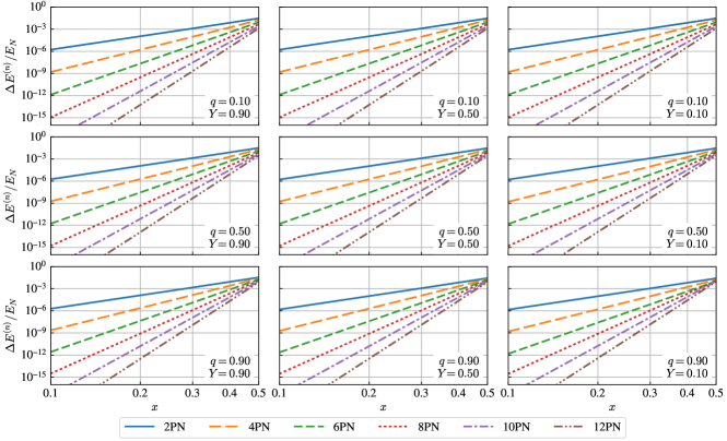
Figure 1: Contribution of each correction term in the PN expansion of the specific energy. We plot $\Delta E^{(n)}$ normalized by the Newtonian energy, $E_{N}$, as functions of $x$ for several sets of $(q,Y)$. To make the plots easier to read, we show only the 2PN ($n=4$), 4PN ($n=8$), 6PN ($n=12$), 8PN ($n=16$), 10PN ($n=20$) and 12PN ($n=24$) corrections in this figure.

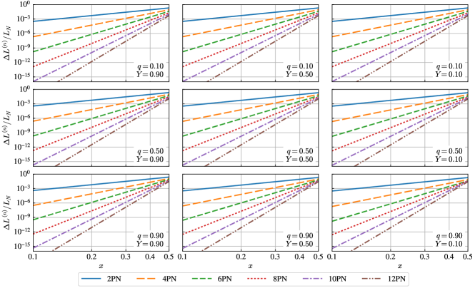
Figure 2: Contribution of each correction term in the PN expansion of the specific angular momentum. We plot $\Delta L^{(n)}$ normalized by the Newtonian term, $L_{N}$, as functions of $x$ for several sets of $(q,Y)$. In the same reason as Fig. 1, we show only the 2PN, 4PN, 6PN, 8PN, 10PN and 12PN corrections in this figure.

IV.2 Convergence of PN formulas for $\dot{E}$ and $\dot{L}$

In a similar manner to Eq. (63), we check the convergence of the PN formulas of $\dot{E}$ and $\dot{L}$ by introducing the difference

$$\Delta\dot{E}^{(n)}\equiv\left|\dot{E}^{(n)}-\dot{E}^{(n-1)}\right|,\quad\Delta\dot{L}^{(n)}\equiv\left|\dot{L}^{(n)}-\dot{L}^{(n-1)}\right|.$$ (64)

In Figs. 3 and 4, we show $\Delta\dot{E}^{(n)}$ and $\Delta\dot{L}^{(n)}$ as functions of $x$ for several sets of $(q,Y)$. We find some spike bottoms which are caused by the logarithmic terms appearing in the PN formulas. Unlike $E$ and $L$, it is difficult to find any tendency in the convergence of $\dot{E}$ and $\dot{L}$ depending on $q$ and $Y$. The convergence is not uniform comparing to $E^{(n)}$ and $L^{(n)}$, but $\Delta\dot{E}^{(n)}$ and $\Delta\dot{L}^{(n)}$ tend to decrease when the PN order increases. Therefore, we expect to obtain more accurate approximants at higher PN order. It is noted that the convergence of $\Delta\dot{E}^{(n)}$ and $\Delta\dot{L}^{(n)}$ may be improved by using resummation technique [22], although we do not deal with this topic in this paper.

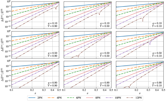
Figure 3: Contribution of each correction term in the PN expansion of $\dot{E}$. We plot $\Delta\dot{E}^{(n)}$ normalized by the leading term, $\dot{E}^{(0)}$, as functions of $x$ for several sets of $(q,Y)$. In the same reason as Fig. 1, we show only the 2PN, 4PN, 6PN, 8PN, 10PN and 12PN corrections in this figure.

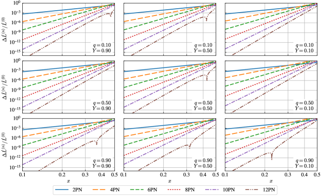
Figure 4: Contribution of each correction term in the PN expansion of $\dot{L}$. We plot $\Delta\dot{L}^{(n)}$ normalized by the leading term, $\dot{L}^{(0)}$, as functions of $x$ for several sets of $(q,Y)$. In the same reason as Fig. 1, we show only the 2PN, 4PN, 6PN, 8PN, 10PN and 12PN corrections in this figure.

IV.3 Comparison of the time-domain Taylor approximants

In a similar manner to Eq. (63), we introduce the difference in the phase between two PN formulas with different order of $x$ for each TaylorT approximant:

$$\Delta\Phi_{X}^{(n)}\equiv\left|\Phi_{X}^{(n)}-\Phi_{X}^{(n-1)}\right|,$$ (65)

where the index $X=$ {T1, T2, T3, T4, T1a, T4a} shows the name of the considered approximant.

Figures 5–9 show $\Delta\Phi_{X}^{(n)}$ of each approximant as functions of time (in unit of month) for several sets of $(q,Y_{I})$ in System1. We find in all cases of $(q,Y_{I})$ that the TaylorT1 shows best convergence. The convergence of the TaylorT1a (TaylorT4a) is almost same as the TaylorT1 (TaylorT4). This suggests that the PN formula of $Y$, Eq. (35), converges well. The TaylorT2 approximant also shows good performance though the convergence is slightly slower than the TaylorT1. The convergence of the TaylorT3 and TaylorT4 is not good comparing to TaylorT1 and TaylorT2. Especially, the TaylorT3 shows poor convergence comparing to the other approximants. This trend is consistent with the result for circular orbits in Schwarzschild case [29]. The convergence of TaylorT3 and TaylorT4 gets slightly better when $q$ and $Y_{I}$ are smaller.

In all plots of Figs. 5–9, we show the line with $\Delta\Phi_{X}^{(n)}=0.1$ as a reference, which corresponds to the statistical error of the phase estimated by $\langle\Delta\Phi\rangle\sim 1/\rho$ with $\rho\simeq 20$ ($\rho$ is the signal-to-noise ratio (SNR)) [33, 34, 35]. As for the TaylorT1 approximant, the 8PN correction of the phase is less than $O(0.1)$ for two years since the GW observation starts for all cases of System1, while the 9th or higher PN corrections in the TaylorT2 are required to suppress the dephasing to $O(0.1)$. Roughly speaking, the following two higher order corrections are needed to obtain the comparable accuracy by using the TaylorT2 approximant instead of the TaylorT1.

We show the results for System2 in Figs. 10–12. In the case of System2, even the 12PN correction, the highest order term we have in hand currently, cannot keep the dephasing less than $O(0.1)$ for two years. This is expected because System2 corresponds to the late stage of a inspiral just before plunging into the central black hole, where the PN convergence gets worse. The tendency of the slow convergence is more pronounced for the TaylorT3 and TaylorT4 approximants. Figures 10–12 do not include the results for the TaylorT3 approximant because the values are far from the other approximants in the case of System2 and the comparison does not make sense.) The reason has been discussed for circular orbit in Schwarzschild case [29]: the slow PN convergence in the late inspiral is attributed to the pole of $(dE/dx)^{-1}$ at the last stable orbit (LSO). In a similar manner, the inverse of the Jacobian, $G^{A}_{B}$, appearing in Eqs. (17) and (18), is expected to have a pole at the LSO, and the PN convergence is slow near the pole. Some techniques of resummation or factorization may be required to improve the slow convergence around the LSO [36, 37].

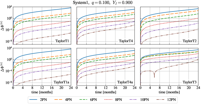
Figure 5: Difference of the phase evolution, $\Delta\Phi_{X}^{(n)}$, for several TaylorT approximants in System1 with $q=0.1$ and $Y_{I}=0.9$. The horizontal dotted line denotes $\Delta\Phi_{X}^{(n)}=10^{-1}$.

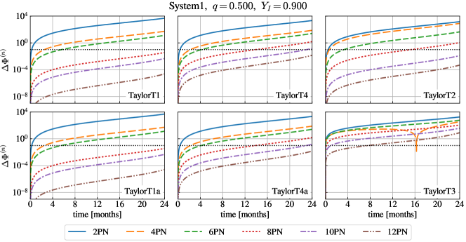
Figure 6: Difference of the phase evolution, $\Delta\Phi_{X}^{(n)}$, for several TaylorT approximants in System1 with $q=0.5$ and $Y_{I}=0.9$. The horizontal dotted line denotes $\Delta\Phi_{X}^{(n)}=10^{-1}$.

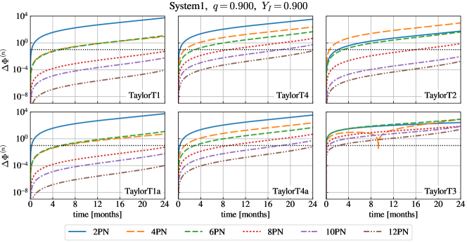
Figure 7: Difference of the phase evolution, $\Delta\Phi_{X}^{(n)}$, for several TaylorT approximants in System1 with $q=0.9$ and $Y_{I}=0.9$. The horizontal dotted line denotes $\Delta\Phi_{X}^{(n)}=10^{-1}$.

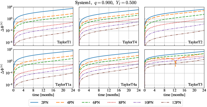
Figure 8: Difference of the phase evolution, $\Delta\Phi_{X}^{(n)}$, for several TaylorT approximants in System1 with $q=0.9$ and $Y_{I}=0.5$. The horizontal dotted line denotes $\Delta\Phi_{X}^{(n)}=10^{-1}$.

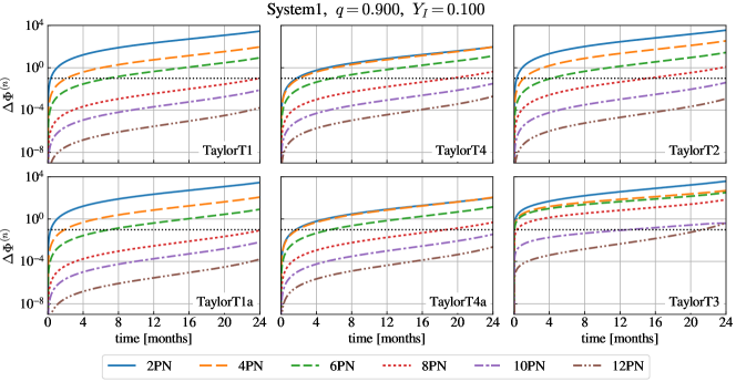
Figure 9: Difference of the phase evolution, $\Delta\Phi_{X}^{(n)}$, for several TaylorT approximants in System1 with $q=0.9$ and $Y_{I}=0.1$. The horizontal dotted line denotes $\Delta\Phi_{X}^{(n)}=10^{-1}$.

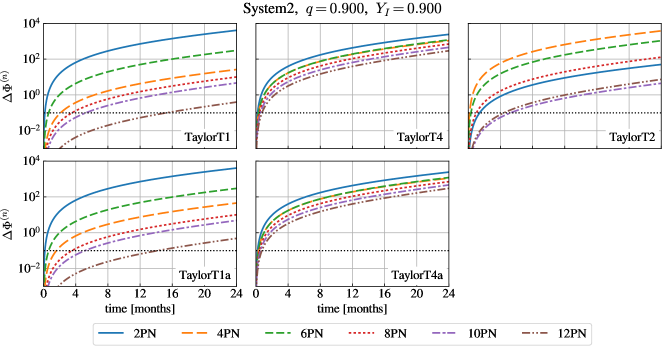
Figure 10: Difference of the phase evolution, $\Delta\Phi_{X}^{(n)}$, for several TaylorT approximants in System2 with $q=0.9$ and $Y_{I}=0.9$. The horizontal dotted line denotes $\Delta\Phi_{X}^{(n)}=10^{-1}$. The plot of the TaylorT3 approximants is not shown because most of them are out of the common range with the other approximants, $10^{-3}\leq\Delta\Phi^{(n)}\leq 10^{4}$, and the comparison does not make sense.

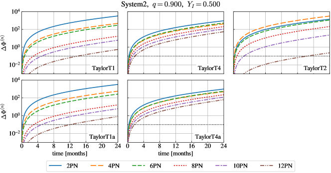
Figure 11: Difference of the phase evolution, $\Delta\Phi_{X}^{(n)}$, for several TaylorT approximants in System2 with $q=0.9$ and $Y_{I}=0.5$. The horizontal dotted line denotes $\Delta\Phi_{X}^{(n)}=10^{-1}$.

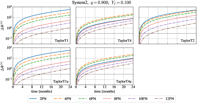
Figure 12: Difference of the phase evolution, $\Delta\Phi_{X}^{(n)}$, for several TaylorT approximants in System2 with $q=0.9$ and $Y_{I}=0.1$. The horizontal dotted line denotes $\Delta\Phi_{X}^{(n)}=10^{-1}$.

IV.4 Performance of the frequency-domain Taylor approximants

To discuss the convergence of the TaylorF2 approximants, it is useful to introduce the overlap between two waveforms, $h_{1}(t)$ and $h_{2}(t)$,

$$\mathcal{O}(h_{1}|h_{2})\equiv\max_{\Delta t}\frac{\left|(h_{1}|h_{2})\right|}{\sqrt{(h_{1}|h_{1})(h_{2}|h_{2})}},$$ (66)

where $\Delta t$ is the time lag between two waveforms. The inner product, $(h_{1}|h_{2})$, is defined by

$$(h_{1}|h_{2})\equiv 2\int_{-\infty}^{\infty}\frac{\tilde{h}_{1}(f)\tilde{h}_{2}^{*}(f)}{S_{n}(f)}df,$$

with the Fourier transforms of $h_{1}(t)$ and $h_{2}(t)$, $\tilde{h}_{1}(f)$ and $\tilde{h}_{2}(f)$, respectively, and the noise power spectral density of GW detector, $S_{n}(f)$. In our current calculation, we use $S_{n}(f)$ for LISA given in Ref. [38]. The overlap becomes the maximum value, unity, when the two waveforms coincide perfectly up to the overall amplitudes.

By using the overlap, we introduce the mismatch between two TaylorF2 approximants with successive orders of $x$ as

$$\mathcal{M}_{\textrm{F2}}^{(n)}\equiv 1-\mathcal{O}(h_{\textrm{F2}}^{(n)}|h_{\textrm{F2}}^{(n-1)}).$$ (67)

$\mathcal{M}_{\textrm{F2}}^{(n)}$ corresponds to the mismatch induced by the correction of $O(x^{n})$. Hence, if the mismatch tends to decrease as the value of $n$ increase, we diagnose that the approximants converge.

In Figs. 13 and 14, we show the mismatch as a function of observation time. We also show the line with $\mathcal{M}_{\textrm{F2}}^{(n)}=10^{-3}$. This corresponds to the limit of mismatch so that two waveforms are indistinguishable, which is estimated by $\mathcal{M}\sim 1/(2\rho^{2})$ with the SNR of $\rho\simeq 20$, and roughly corresponds to the dephasing of $\Delta\Phi\sim O(0.1)$ in time-domain templates [34, 35, 39]. For System1 (early stage of inspiral), the 8PN order approximant keeps the mismatch less than $O(0.01)$ for two-year observation, but it is not sufficient to suppress the mismatch to $O(10^{-3})$. The 9th or higher PN order approximants are required. The performance of the TaylorF2 approximant is similar to the TaylorT2 in the time-domain families. As shown in Sec. IV.3, the 9th or higher PN TaylorT2 approximants are required to suppress the dephasing to $O(0.1)$ (corresponding to a $O(10^{-3})$ mismatch in the frequency domain) for two years. This fact may be expected from the similarity in the formulation of the TaylorT2 and TaylorF2 approximants.

For System2 (late stage of inspiral), even the 12PN approximants, which is the highest order we have currently, does not keep the mismatch less than $O(10^{-3})$ for two years. This tendency is same as we show for the phase evolution in the TaylorT families.

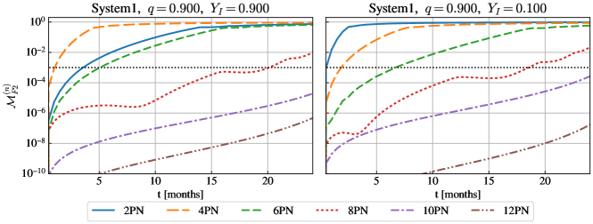
Figure 13: Mismatch between different PN order TaylorF2 approximants, $\mathcal{M}_{\textrm{F2}}^{(n)}$ for System1 with $q=0.9$. The horizontal dotted line denotes $\mathcal{M}_{\textrm{F2}}^{(n)}=10^{-3}$.

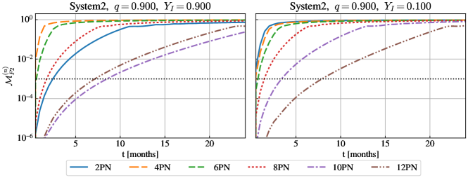
Figure 14: Mismatch between different PN order TaylorF2 approximants, $\mathcal{M}_{\textrm{F2}}^{(n)}$ for System2 with $q=0.9$. The horizontal dotted line denotes $\mathcal{M}_{\textrm{F2}}^{(n)}=10^{-3}$.

V Summary

In this work, we presented various PN template families for the phase evolution of quasi-spherical EMRIs in Kerr spacetime and examine the convergence by evaluating the dephasing between approximants with different PN orders belonging to each family. We found that the PN convergence slightly depends on the black hole spin, $q$, and the initial value of the inclination, $Y_{I}$, and that the convergence gets slow when $q$ or $Y_{I}$ becomes large. This tendency implies that the rotation of the central black hole works to slow the convergence. In addition, the tendency suggests that we may focus on the cases with larger $q$ and larger $Y_{I}$ (the case of $Y_{I}=0.9$ and $q=0.9$ in the current work) to discuss the convergence of various approximants.

From the comparison of TaylorT families, we found that the TaylorT1 approximant shows the best performance among them as shown for circular orbits in Schwarzschild case [29]. For early inspirals (represented by System1), the 8PN TaylorT1 template is expected to keep the dephasing less than $O(0.1)$ during two-year observation. The alternative approximant of the TaylorT1, named TaylorT1a in this work, shows the equivalent performance too. As for the TaylorT2 template, the corrections at least up to the 9PN order will be required to achieve the comparable accuracy to the TaylorT1. Although the convergence of the TaylorT2 approximant is slightly slower than that of the TaylorT1/T1a, however, the fully analytical expression is useful to reduce the computational cost to construct the bank of GW templates and to discuss effects beyond general relativity.

To examine the convergence of the TaylorF2 approximant, we evaluated the mismatch between templates with different PN orders. For early inspirals, the corrections at least up to 9PN order will be required to keep the mismatch to $O(10^{-3})$, which corresponds to the dephasing of $O(0.1)$ in the time domain. This results supports the expectation that the TaylorF2 approximant has comparable performance to the TaylorT2 from the similarity in the formulation. Since the TaylorF2 approximant is given in fully analytical expression same as the TaylorT2, it provides an easy-to-handle method of calculating the frequency-domain templates for EMRIs.

For late inspirals (represented by System2), the performance of all PN approximants considered in this work gets worse than that for early inspirals. It is a natural result because $x$, which is used as the PN parameter, becomes large as the inspiralling object approaches the central black hole, and accordingly the convergence of the expansion with respect to $x$ becomes slow. Even the best template in this work, the 12PN TaylorT1 approximant, cannot keep the dephasing to $O(0.1)$ for two years. To satisfy $\Delta\Phi_{X}^{(n)}\leq 10^{-1}$ for the GW observation of System2, higher PN (at least 14PN deducing from the Schwarzschild case [29]) order calculation will be required. There have been several efforts to improve the convergence of the energy flux by using the factorization and resummation of the PN expansion so far [36, 40, 41, 42, 43, 22]. The extension of the factorization and resummation to the spherical (and generic bound) orbits may be studied as a future work.

In this work, we restricted binaries to the case of $e=0$. In general, it is expected that several EMRIs in the universe have finite eccentricity when the GWs emitted by them come into the frequency band in which LISA can detect. The extension of the current work to generic bound orbits with three orbital parameters is necessary to aim the GWs from EMRIs with a broad range of parameters. The extension of the TaylorT1 and TaylorT4 families is trivial, while the derivation of the full analytical approximants, the TaylorT2, TaylorT3, and TaylorF2, will be more complicated than the spherical orbit case [19]. Further investigation is needed to accomplish it.

Throughout this paper, we focus only on the dephasing in the orbital phase of $\varphi$-direction (i.e., the rotation angle). For spherical orbits, however, the phase with respect to $\theta$ (corresponds to the libration angle variable of polar motion) exists, which induces GWs with other harmonics in terms of the linear combination of orbital and polar frequencies. For generic bound orbits in Kerr spacetime, there is another phase with respect to the radial direction. We will work on the derivation of the PN templates for the additional phases and harmonics in future.

Appendix A Expansion coefficients of the specific energy and angular momentum

The expansion coefficients in Eqs. (20) and (21) up to $O(x^{9})$ are given as

$$\tilde{E}_{0} = 1,\quad\tilde{E}_{1}=0,\quad\tilde{E}_{2}=-\frac{3}{4},\quad\tilde{E}_{3}=\left(-\frac{4}{3}+4\,Y\right)q,$$

$$\tilde{E}_{4} = -{\frac{27}{8}}+\left(\frac{1}{2}+Y-\frac{5}{2}\,{Y}^{2}\right){q}^{2},\quad\tilde{E}_{5}=\left(2+6\,Y\right)q,$$

$$\tilde{E}_{6} = -{\frac{675}{64}}+\left({\frac{341}{36}}-{\frac{137\,Y}{6}}+{\frac{39\,{Y}^{2}}{4}}\right){q}^{2},$$

$$\tilde{E}_{7} = \left({\frac{27}{2}}+{\frac{27\,Y}{2}}\right)q+\left(-2-9\,Y+32\,{Y}^{2}-21\,{Y}^{3}\right){q}^{3},$$

$$\tilde{E}_{8} = -{\frac{3969}{128}}+\left({\frac{109}{48}}-{\frac{209\,Y}{8}}+{\frac{69\,{Y}^{2}}{16}}\right){q}^{2}+\left({\frac{21}{32}}+{\frac{19\,Y}{8}}-{\frac{9\,{Y}^{2}}{16}}-{\frac{101\,{Y}^{3}}{8}}+{\frac{325\,{Y}^{4}}{32}}\right){q}^{4},$$

$$\tilde{E}_{9} = \left({\frac{225}{4}}+{\frac{135\,Y}{4}}\right)q+\left(-{\frac{4208}{81}}+{\frac{3055\,Y}{18}}-185\,{Y}^{2}+{\frac{433\,{Y}^{3}}{6}}\right){q}^{3},$$

$$\tilde{L}_{0} = 1,\quad\tilde{L}_{1}=0,\quad\tilde{L}_{2}=\frac{3}{2},\quad\tilde{L}_{3}=\left(\frac{2}{3}-4\,Y\right)q,$$

$$\tilde{L}_{4} = \frac{27}{8}+\left(-\frac{1}{4}-\frac{Y}{2}+\frac{7}{4}\,{Y}^{2}\right){q}^{2},\quad\tilde{L}_{5}=\left(-1-6\,Y\right)q,$$

$$\tilde{L}_{6} = {\frac{135}{16}}+\left(-{\frac{437}{72}}+{\frac{121\,Y}{12}}-{\frac{9\,{Y}^{2}}{8}}\right){q}^{2},$$

$$\tilde{L}_{7} = \left(-{\frac{27}{4}}-{\frac{27\,Y}{2}}\right)q+\left(\frac{1}{2}+6\,Y-{\frac{27\,{Y}^{2}}{2}}+7\,{Y}^{3}\right){q}^{3},$$

$$\tilde{L}_{8} = {\frac{2835}{128}}+\left(-{\frac{493}{96}}+{\frac{241\,Y}{16}}+{\frac{129\,{Y}^{2}}{32}}\right){q}^{2}+\left(-{\frac{15}{64}}-{\frac{13\,Y}{16}}-{\frac{13\,{Y}^{2}}{32}}+{\frac{83\,{Y}^{3}}{16}}-{\frac{239\,{Y}^{4}}{64}}\right){q}^{4},$$

$$\tilde{L}_{9} = \left(-{\frac{225}{8}}-{\frac{135\,Y}{4}}\right)q+\left({\frac{7747}{324}}-{\frac{578\,Y}{9}}+{\frac{243\,{Y}^{2}}{4}}-{\frac{143\,{Y}^{3}}{6}}\right){q}^{3}.$$

Appendix B Expansion coefficients of $\dot{E}$ and $\dot{L}$

The expansion coefficients in Eqs. (22) and (23) up to $O(x^{9})$ are given as

$$\tilde{\dot{E}}_{0} = 1,\quad\tilde{\dot{E}}_{1}=0,\quad\tilde{\dot{E}}_{2}=-{\frac{1247}{336}},\quad\tilde{\dot{E}}_{3}=4\pi+\left(-\frac{20}{3}+\frac{47Y}{12}\right)q,$$

$$\tilde{\dot{E}}_{4} = -\frac{44711}{9072}+\left(-\frac{89}{96}+5Y-\frac{193}{96}Y^{2}\right)q^{2},$$

$$\tilde{\dot{E}}_{5} = -\frac{8191\pi}{672}+\left(\frac{1247}{42}-\frac{11299Y}{336}\right)q+\left(-\frac{9}{32}Y-\frac{15}{32}Y^{3}\right)q^{3},$$

$$\tilde{\dot{E}}_{6} = -\frac{3424\ln\!\left(2\right)}{105}+\frac{16\pi^{2}}{3}-\frac{1712\ln x}{105}-\frac{1712\gamma}{105}+\frac{6643739519}{69854400}+\left(-\frac{104}{3}\pi+\frac{143}{6}\pi Y\right)q$$

$$+\left(\frac{55067}{1008}-\frac{48491}{504}Y+\frac{4793}{112}Y^{2}\right)q^{2},$$

$$\tilde{\dot{E}}_{7} = -\frac{16285\pi}{504}+\left(\frac{44711}{972}-\frac{6899Y}{1296}\right)q-\frac{\left(185-1248Y+673Y^{2}\right)\pi\,q^{2}}{48}$$

$$+\left(\frac{623}{72}-\frac{2643}{32}Y+\frac{938}{9}Y^{2}-\frac{3389}{96}Y^{3}\right)q^{3},$$

$$\tilde{\dot{E}}_{8} = \frac{39931\ln\!\left(2\right)}{294}-\frac{47385\ln\!\left(3\right)}{1568}-\frac{1369\pi^{2}}{126}+\frac{232597\ln x}{4410}+\frac{232597\gamma}{4410}+\frac{\kappa}{2}-\frac{321516361867}{3178375200}$$

$$+\left[\left(\frac{1}{2}-\frac{Y^{4}}{2}\right)\Psi_{B}^{(0,1)}(q)+\left(\frac{1}{4}+\frac{3}{2}Y^{2}+\frac{1}{4}Y^{4}\right)\Psi_{B}^{(0,2)}(q)+\frac{40955\pi}{336}-\frac{49571\pi Y}{336}\right]q$$

$$+\left[\frac{7\kappa}{8}-\frac{2501753}{9072}+\frac{4353865Y}{9072}+\frac{\left(51030\kappa-1753858\right)Y^{2}}{9072}\right]q^{2}$$

$$+\left[\left(-\frac{3}{8}+\frac{3Y^{4}}{8}\right)\Psi_{B}^{(0,1)}(q)+\left(\frac{3}{4}+\frac{9}{2}Y^{2}+\frac{3}{4}Y^{4}\right)\Psi_{B}^{(0,2)}(q)\right]q^{3}$$

$$+\left[\frac{3\kappa}{16}+\frac{1485}{256}+\frac{67Y}{96}+\frac{\left(1440\kappa+10562\right)Y^{2}}{768}-\frac{3361Y^{3}}{96}+\frac{\left(720\kappa+11959\right)Y^{4}}{768}\right]q^{4},$$

$$\tilde{\dot{E}}_{9} = -\frac{6848\pi}{105}\left(2\ln\!\left(2\right)+\ln x+\gamma-\frac{265978667519}{48595599360}\right)$$

$$+\Biggl{[}\frac{18223349760-11414375280Y}{52390800}\ln(2)-\frac{512\pi^{2}}{9}+\frac{54784\ln x}{315}+\frac{54784\gamma}{315}-\frac{6572554559}{6548850}$$

$$+\frac{\left(2229519600\pi^{2}-5698289520\gamma-5698289520\ln x+42430399563\right)Y}{52390800}\Biggr{]}q$$

$$+\frac{\pi\left(1305107-2232275Y+977850Y^{2}\right)q^{2}}{4032}+\left(-\frac{240382}{567}+\frac{16357489}{12096}Y-\frac{326943}{224}Y^{2}+\frac{220719}{448}Y^{3}\right)q^{3}$$

$$+\left(-\frac{1083}{1792}Y-\frac{135}{64}Y^{2}+\frac{211}{128}Y^{3}-\frac{225}{64}Y^{4}+\frac{1095}{256}Y^{5}\right)q^{5},$$

$$\tilde{\dot{L}}_{0} = Y,\quad\tilde{\dot{L}}_{1}=0,\quad\tilde{\dot{L}}_{2}=-{\frac{1247\,Y}{336}},\quad\tilde{\dot{L}}_{3}=4\,\pi\,Y+\left({\frac{61}{24}}-\frac{14}{3}\,Y-\frac{5}{8}\,{Y}^{2}\right)q,$$

$$\tilde{\dot{L}}_{4} = -{\frac{44711\,Y}{9072}}+\left(-{\frac{29\,Y}{16}}+\frac{7}{2}\,{Y}^{2}+\frac{3}{8}\,{Y}^{3}\right){q}^{2},$$

$$\tilde{\dot{L}}_{5} = -{\frac{8191\,\pi\,Y}{672}}+\left(-{\frac{2661}{224}}+{\frac{1247\,Y}{56}}-{\frac{3209\,{Y}^{2}}{224}}\right)q+\left(-{\frac{33}{128}}-{\frac{9\,{Y}^{2}}{64}}-{\frac{45\,{Y}^{4}}{128}}\right){q}^{3},$$

$$\tilde{\dot{L}}_{6} = -{\frac{1712\,\ln x\,Y}{105}}+\frac{16}{3}\,{\pi}^{2}Y-{\frac{1712\,\gamma\,Y}{105}}-{\frac{3424\,\ln\left(2\right)Y}{105}}+{\frac{6643739519\,Y}{69854400}}$$

$$+\left({\frac{145\,\pi}{12}}-{\frac{80\,\pi\,Y}{3}}+{\frac{15\,\pi\,{Y}^{2}}{4}}\right)q+\left(-{\frac{305}{18}}+{\frac{181823\,Y}{4032}}-{\frac{27239\,{Y}^{2}}{672}}+{\frac{6091\,{Y}^{3}}{448}}\right){q}^{2},$$

$$\tilde{\dot{L}}_{7} = -{\frac{16285\,\pi\,Y}{504}}+\left(-{\frac{80123}{6048}}+{\frac{491821\,Y}{13608}}+{\frac{322627\,{Y}^{2}}{18144}}\right)q+\left(-{\frac{71\,\pi\,Y}{8}}+20\,\pi\,{Y}^{2}-3\,\pi\,{Y}^{3}\right){q}^{2}$$

$$+\left(-{\frac{377}{128}}+26\,Y-{\frac{10645\,{Y}^{2}}{192}}+{\frac{289\,{Y}^{3}}{8}}-{\frac{1121\,{Y}^{4}}{128}}\right){q}^{3},$$

$$\tilde{\dot{L}}_{8} = {\frac{232597\,\ln x\,Y}{4410}}-{\frac{321516361867\,Y}{3178375200}}+\frac{1}{2}\,\kappa\,Y-{\frac{47385\,\ln\left(3\right)Y}{1568}}-{\frac{1369\,{\pi}^{2}Y}{126}}+{\frac{232597\,\gamma\,Y}{4410}}+{\frac{39931\,\ln\left(2\right)Y}{294}}$$

$$+\left[\left(\frac{Y}{2}-\frac{1}{2}\,{Y}^{3}\right)\Psi_{B}^{(0,1)}(q)+\left(Y+{Y}^{3}\right)\Psi_{B}^{(0,2)}(q)-{\frac{16481\,\pi}{336}}+{\frac{8191\,\pi\,Y}{84}}-{\frac{3557\,\pi\,{Y}^{2}}{48}}\right]q$$

$$+\left({\frac{2661}{28}}-{\frac{8954023\,Y}{36288}}+{\frac{59\,\kappa\,Y}{16}}+{\frac{4011779\,{Y}^{2}}{18144}}-{\frac{2125175\,{Y}^{3}}{36288}}+{\frac{45\,\kappa\,{Y}^{3}}{16}}\right){q}^{2}$$

$$+\left[\left(-\frac{3}{8}\,Y+\frac{3}{8}\,{Y}^{3}\right)\Psi_{B}^{(0,1)}(q)+\left(3\,Y+3\,{Y}^{3}\right)\Psi_{B}^{(0,2)}(q)\right]{q}^{3}$$

$$+\left({\frac{33}{16}}+{\frac{31\,Y}{64}}+{\frac{9\,\kappa\,Y}{8}}-{\frac{185\,{Y}^{2}}{32}}+{\frac{997\,{Y}^{3}}{64}}+{\frac{15\,\kappa\,{Y}^{3}}{8}}-{\frac{209\,{Y}^{4}}{16}}+{\frac{49\,{Y}^{5}}{32}}\right){q}^{4},$$

$$\tilde{\dot{L}}_{9} = \left[-{\frac{6848\,\pi\,Y}{105}}+\left(-{\frac{32699}{630}}+{\frac{44512\,Y}{315}}-{\frac{5093\,{Y}^{2}}{210}}\right)q\right]\ln x-{\frac{13696\,\ln\left(2\right)\pi\,Y}{105}}-{\frac{6848\,\gamma\,\pi\,Y}{105}}$$

$$+{\frac{265978667519\,\pi\,Y}{745113600}}+\biggl{(}{\frac{22634193223}{69854400}}+{\frac{337\,{\pi}^{2}}{18}}-{\frac{65291\,\ln\left(2\right)}{630}}-{\frac{32699\,\gamma}{630}}-{\frac{85229654387\,Y}{104781600}}-{\frac{416\,{\pi}^{2}Y}{9}}$$

$$+{\frac{89024\,\ln\left(2\right)Y}{315}}+{\frac{44512\,\gamma\,Y}{315}}+{\frac{79\,{\pi}^{2}{Y}^{2}}{6}}-{\frac{5093\,\gamma\,{Y}^{2}}{210}}-{\frac{3431\,\ln\left(2\right){Y}^{2}}{70}}+{\frac{20652193823\,{Y}^{2}}{69854400}}\biggr{)}q$$

$$+\left(-{\frac{1885\,\pi}{18}}+{\frac{1198205\,\pi\,Y}{4032}}-{\frac{29751\,\pi\,{Y}^{2}}{112}}+{\frac{38417\,\pi\,{Y}^{3}}{448}}\right){q}^{2}$$

$$+\left({\frac{5006923}{48384}}-{\frac{9190967\,Y}{18144}}+{\frac{6411011\,{Y}^{2}}{8064}}-{\frac{55219\,{Y}^{3}}{96}}+{\frac{777995\,{Y}^{4}}{5376}}\right){q}^{3}$$

$$+\left(-{\frac{549}{896}}-{\frac{99\,Y}{64}}+{\frac{2955\,{Y}^{2}}{1792}}-{\frac{27\,{Y}^{3}}{32}}+{\frac{3\,{Y}^{4}}{32}}-{\frac{135\,{Y}^{5}}{64}}+{\frac{785\,{Y}^{6}}{256}}\right){q}^{5},$$

where $\gamma=0.5772156649\cdots$ is the Euler’s constant, $\kappa=\sqrt{1-q^{2}}$, and $\Psi_{A}^{(n,m)}(q)$ and $\Psi_{B}^{(n,m)}(q)$ are real functions defined by the polygamma function $\psi^{(n)}(z)$ as

$$\Psi_{A}^{(n,m)}(q) \equiv \frac{1}{2}\left[\psi^{(n)}\left(3+\frac{imq}{\sqrt{1-q^{2}}}\right)+\psi^{(n)}\left(3-\frac{imq}{\sqrt{1-q^{2}}}\right)\right],$$ (68)

$$\Psi_{B}^{(n,m)}(q) \equiv \frac{1}{2i}\left[\psi^{(n)}\left(3+\frac{imq}{\sqrt{1-q^{2}}}\right)-\psi^{(n)}\left(3-\frac{imq}{\sqrt{1-q^{2}}}\right)\right].$$ (69)

Appendix C Expansion coefficients, $\tilde{\dot{x}}_{k}$ and $\tilde{\dot{Y}}_{k}$, in Eqs. (27) and (29)

The expansion coefficients in Eqs. (27) and (29) for $k\leq 9$ are given as

$$\tilde{\dot{x}}_{0} = 1,\quad\tilde{\dot{x}}_{1}=0,\quad\tilde{\dot{x}}_{2}=-{\frac{743}{336}},\quad\tilde{\dot{x}}_{3}=4\pi+\left(-\frac{10}{3}-\frac{73Y}{12}\right)q,$$

$$\tilde{\dot{x}}_{4} = \frac{34103}{18144}+\left(-\frac{233}{96}+2Y+\frac{527}{96}Y^{2}\right)q^{2},$$

$$\tilde{\dot{x}}_{5} = -\frac{4159\pi}{672}+\left(\frac{743}{72}-\frac{13991Y}{336}\right)q+\left(-\frac{9}{32}Y-\frac{15}{32}Y^{3}\right)q^{3},$$

$$\tilde{\dot{x}}_{6} = -\frac{3424\ln\!\left(2\right)}{105}+\frac{16\pi^{2}}{3}-\frac{1712\ln x}{105}-\frac{1712\gamma}{105}+\frac{16447322263}{139708800}$$

$$+\left(-\frac{64}{3}\pi-\frac{97}{6}\pi Y\right)q+\left(\frac{41891}{4032}+\frac{17953}{1008}Y+\frac{22935}{448}Y^{2}\right)q^{2},$$

$$\tilde{\dot{x}}_{7} = -\frac{4415\pi}{4032}+\left(-\frac{34103}{3024}-\frac{54595Y}{336}\right)q+\frac{\pi\left(-473+672Y+767Y^{2}\right)q^{2}}{48}$$

$$+\left(\frac{95}{6}+\frac{59}{64}Y-\frac{99}{2}Y^{2}-\frac{6797}{192}Y^{3}\right)q^{3},$$

$$\tilde{\dot{x}}_{8} = \frac{127751\ln\!\left(2\right)}{1470}-\frac{47385\ln\!\left(3\right)}{1568}-\frac{361\pi^{2}}{126}+\frac{124741\ln x}{4410}+\frac{124741\gamma}{4410}+\frac{\kappa}{2}+\frac{3971984677513}{25427001600}$$

$$+\left[\left(\frac{1}{2}-\frac{Y^{4}}{2}\right)\Psi_{B}^{(0,1)}(q)+\left(\frac{1}{4}+\frac{3}{2}Y^{2}+\frac{1}{4}Y^{4}\right)\Psi_{B}^{(0,2)}(q)+\frac{20795\pi}{504}-\frac{5429\pi Y}{28}\right]q$$

$$+\left[\frac{7\kappa}{8}-\frac{26297639}{145152}+\frac{207683Y}{648}+\frac{\left(816480\kappa+85019873\right)Y^{2}}{145152}\right]q^{2}$$

$$+\left[\left(-\frac{3}{8}+\frac{3Y^{4}}{8}\right)\Psi_{B}^{(0,1)}(q)+\left(\frac{3}{4}+\frac{9}{2}Y^{2}+\frac{3}{4}Y^{4}\right)\Psi_{B}^{(0,2)}(q)\right]q^{3}$$

$$+\left[\frac{3\kappa}{16}+\frac{1445}{256}-\frac{1517Y}{192}+\frac{\left(1440\kappa-9554\right)Y^{2}}{768}+\frac{4829Y^{3}}{192}+\frac{\left(720\kappa+8099\right)Y^{4}}{768}\right]q^{4},$$

$$\tilde{\dot{x}}_{9} = -\frac{6848\pi}{105}\left(\ln x+2\ln\!\left(2\right)+\gamma-\frac{343801320119}{48595599360}\right)$$

$$+\Biggl{[}\frac{\left(100228423680+45360120960Y\right)\ln\!\left(2\right)}{419126400}+\frac{\left(50114211840+22751245440Y\right)\ln x}{419126400}$$

$$-\frac{352\pi^{2}}{9}+\frac{37664\gamma}{315}-\frac{16240238743}{19051200}+\frac{\left(-4517251200\pi^{2}+22751245440\gamma-578438815461\right)Y}{419126400}\Biggr{]}q$$

$$+\frac{\left(482588+43163Y+812745Y^{2}\right)\pi\,q^{2}}{4032}+\left(-\frac{1672145}{36288}+\frac{18305605}{48384}Y-\frac{584543}{1344}Y^{2}-\frac{1745175}{1792}Y^{3}\right)q^{3}$$

$$+\left(-\frac{33}{256}+\frac{207}{448}Y-\frac{153}{128}Y^{2}-\frac{7}{64}Y^{3}-\frac{525}{256}Y^{4}+\frac{15}{32}Y^{5}\right)q^{5},$$

$$\tilde{\dot{Y}}_{0} = 0,\quad\tilde{\dot{Y}}_{1}=0,\quad\tilde{\dot{Y}}_{2}=0,$$

$$\tilde{\dot{Y}}_{3} = 1,\quad\tilde{\dot{Y}}_{4}=-\frac{13Yq}{244},\quad\tilde{\dot{Y}}_{5}=-\frac{10545}{1708}+\left(-\frac{99}{976}-\frac{45Y^{2}}{976}\right)q^{2},$$

$$\tilde{\dot{Y}}_{6} = \frac{290\pi}{61}+\left(-\frac{22}{3}+\frac{24821Y}{3416}\right)q,\quad\tilde{\dot{Y}}_{7}=\frac{5177}{7686}-\frac{97Y\pi q}{122}+\left(-\frac{1477}{1952}+\frac{723}{122}Y-\frac{4867}{1952}Y^{2}\right)q^{2},$$

$$\tilde{\dot{Y}}_{8} = \frac{6Y\left(3+Y^{2}\right)\Psi_{B}^{(0,2)}(q)}{61}-\frac{12Y^{3}}{61}\Psi_{B}^{(0,1)}(q)-\frac{22571\pi}{854}+\left(\frac{45695}{854}+\frac{408240\kappa-20321879}{368928}Y\right)q$$

$$+\left[\frac{18Y\left(3+Y^{2}\right)\Psi_{B}^{(0,2)}(q)}{61}+\frac{9Y^{3}}{61}\Psi_{B}^{(0,1)}(q)\right]q^{2}$$

$$+\left(\frac{429}{488}+\frac{720\kappa-5435}{1952}Y+\frac{39}{488}Y^{2}+\frac{720\kappa+1811}{1952}Y^{3}\right)q^{3},$$

$$\tilde{\dot{Y}}_{9} = -\frac{130796\ln x}{6405}+\frac{1348\pi^{2}}{183}-\frac{261164\ln\!\left(2\right)}{6405}-\frac{130796\gamma}{6405}+\frac{98625105067}{710186400}+\left(-\frac{8120}{183}\pi+\frac{315059}{6832}\pi Y\right)q$$

$$+\left(\frac{3626515}{70272}-\frac{1557155}{10248}Y+\frac{68911}{896}Y^{2}\right)q^{2}+\left(-\frac{7281}{27328}-\frac{1287}{1952}Y+\frac{405}{488}Y^{2}-\frac{585}{1952}Y^{3}+\frac{735}{3904}Y^{4}\right)q^{4}.$$

Appendix D Expansion coefficients in Eq. (35)

The expansion coefficients of $Y(x)$ in Eq. (35), $\tilde{Y}_{k}$, for $k\leq 9$ are given by

$$\tilde{Y}_{3} = {\frac{61}{72}},\quad\tilde{Y}_{4}=-\frac{13\tilde{Y}_{0}q}{384},\quad\tilde{Y}_{5}=-\frac{81217}{40320}-\left(\frac{3\tilde{Y}_{0}^{2}}{128}+\frac{33}{640}\right)q^{2},\quad\tilde{Y}_{6}=\frac{23\pi}{72}+\left(\frac{3671095\tilde{Y}_{0}}{580608}-\frac{61}{36}\right)q,$$

$$\tilde{Y}_{7} = -\frac{617846599}{170698752}-\frac{71\pi\tilde{Y}_{0}q}{336}+\left(-\frac{2824223}{903168}\tilde{Y}_{0}^{2}+\frac{49}{36}\tilde{Y}_{0}+\frac{1467113}{2709504}\right)q^{2},$$

$$\tilde{Y}_{8} = -\frac{\tilde{Y}_{0}^{3}}{16}\Psi_{B}^{(0,1)}(q)+\frac{\tilde{Y}_{0}(\tilde{Y}_{0}^{2}+3)}{32}\Psi_{B}^{(0,2)}(q)-\frac{111617\pi}{129024}+\left(\frac{45}{128}\tilde{Y}_{0}\kappa-\frac{23469357001}{3901685760}\tilde{Y}_{0}+\frac{81217}{12096}\right)q$$

$$+\left[\frac{3\tilde{Y}_{0}^{3}}{64}\Psi_{B}^{(0,1)}(q)+\frac{3\tilde{Y}_{0}(\tilde{Y}_{0}^{2}+3)}{32}\Psi_{B}^{(0,2)}(q)+\frac{15\pi\,\tilde{Y}_{0}^{2}}{256}+\frac{33\pi}{256}\right]q^{2}$$

$$+\left[\frac{11}{64}+\frac{\left(172800\kappa+567235\right)\tilde{Y}_{0}^{3}}{1474560}+\frac{\tilde{Y}_{0}^{2}}{96}+\frac{\left(172800\kappa-1615377\right)\tilde{Y}_{0}}{1474560}\right]q^{3},$$

$$\tilde{Y}_{9} = -\frac{5\pi^{2}}{18}-\frac{2197\gamma}{1890}-\frac{2615\ln\!\left(2\right)}{1134}-\frac{2197\ln x}{1890}+\frac{40135977646837}{20279011737600}$$

$$+\left(\frac{2335369}{580608}\pi\tilde{Y}_{0}-\frac{23}{18}\pi\right)q+\left(\frac{255882808969}{5852528640}\tilde{Y}_{0}^{2}-\frac{3280}{81}\tilde{Y}_{0}+\frac{47697759001}{17557585920}\right)q^{2}$$

$$+\left(\frac{4439}{36864}\tilde{Y}_{0}^{4}-\frac{15}{256}\tilde{Y}_{0}^{3}+\frac{66139}{184320}\tilde{Y}_{0}^{2}-\frac{33}{256}\tilde{Y}_{0}-\frac{93893}{645120}\right)q^{4}.$$

Appendix E Expansion coefficients in $t_{\textrm{T2}}^{(n)}$ and $\Phi_{\textrm{T2}}^{(n)}$

The expansion coefficients in Eqs. (38) and (39), $\tilde{t}_{k}$ and $\tilde{\Phi}_{k}^{\textrm{T2}}$, for $k\leq 9$ are given as

$$\tilde{t}_{0} = 1,\quad\tilde{t}_{1}=0,\quad\tilde{t}_{2}={\frac{743}{252}},\quad\tilde{t}_{3}=-\frac{32\pi}{5}+\left(\frac{16}{3}+\frac{146\tilde{Y}_{0}}{15}\right)q,$$

$$\tilde{t}_{4} = \frac{3058673}{508032}+\left(\frac{233}{48}-4\tilde{Y}_{0}-\frac{527}{48}\tilde{Y}_{0}^{2}\right)q^{2},$$

$$\tilde{t}_{5} = -\frac{7729\pi}{252}+\left(\frac{743}{63}+\frac{138185\tilde{Y}_{0}}{756}\right)q+\left(\frac{3}{4}\tilde{Y}_{0}+\frac{5}{4}\tilde{Y}_{0}^{3}\right)q^{3},$$

$$\tilde{t}_{6} = \frac{6848\ln x}{105}-\frac{10052469856691}{23471078400}+\frac{128\pi^{2}}{3}+\frac{13696\ln\!\left(2\right)}{105}+\frac{6848\gamma}{105}+\left(-\frac{64}{3}\pi-130\pi\tilde{Y}_{0}\right)q$$

$$+\left(\frac{304897}{12096}+\frac{14011}{252}\tilde{Y}_{0}-\frac{1611751}{12096}\tilde{Y}_{0}^{2}\right)q^{2},$$

$$\tilde{t}_{7} = -\frac{15419335\pi}{127008}+\left(\frac{3058673}{190512}+\frac{5035793419\tilde{Y}_{0}}{1524096}\right)q+\frac{\pi(-153+32\tilde{Y}_{0}+447\tilde{Y}_{0}^{2})q^{2}}{2}$$

$$+\left(\frac{49}{3}+\frac{2518475}{12096}\tilde{Y}_{0}-105\tilde{Y}_{0}^{2}-\frac{3756875}{12096}\tilde{Y}_{0}^{3}\right)q^{3},$$

$$\tilde{t}_{8} = \Biggl{\{}-\frac{202204\ln\!\left(2\right)}{441}-\frac{47385\ln\!\left(3\right)}{196}-\frac{18098\pi^{2}}{63}-\frac{36812\gamma}{105}+4\kappa+\frac{2498644552172012833}{461347517030400}$$

$$+\left[(4-4\tilde{Y}_{0}^{4})\Psi_{B}^{(0,1)}(q)+(2+12\tilde{Y}_{0}^{2}+2\tilde{Y}_{0}^{4})\Psi_{B}^{(0,2)}(q)+\frac{141245\pi\tilde{Y}_{0}}{56}\right]q$$

$$+\left[7\kappa-\frac{8416499209}{8709120}+\frac{\left(2743372800\kappa+36138488713\right)\tilde{Y}_{0}^{2}}{60963840}\right]q^{2}$$

$$+\left[(-3+3\tilde{Y}_{0}^{4})\Psi_{B}^{(0,1)}(q)+(6+36\tilde{Y}_{0}^{2}+6\tilde{Y}_{0}^{4})\Psi_{B}^{(0,2)}(q)+18\pi\tilde{Y}_{0}+30\pi\,\tilde{Y}_{0}^{3}\right]q^{3}$$

$$+\left(\frac{3}{2}\kappa-\frac{14819}{5760}+15\kappa\,\tilde{Y}_{0}^{2}+\frac{254401}{3840}\tilde{Y}_{0}^{2}+\frac{15}{2}\kappa\,\tilde{Y}_{0}^{4}-\frac{492385}{2304}\tilde{Y}_{0}^{4}\right)q^{4}\Biggr{\}}\ln x-\frac{18406(\ln x)^{2}}{105},$$

$$\tilde{t}_{9} = \left[\frac{54784\pi}{105}+\left(\frac{27392}{315}-\frac{363112\tilde{Y}_{0}}{315}\right)q\right]\ln x+\frac{512\pi}{3}\left(\pi^{2}+\frac{107\gamma}{35}+\frac{214\ln\left(2\right)}{35}-\frac{102282756713483}{4005730713600}\right)$$

$$+\biggl{[}\frac{(3061522759680-40631789721600\tilde{Y}_{0})\ln\!\left(2\right)}{17603308800}+\frac{512\pi^{2}}{9}+\frac{27392\gamma}{315}-\frac{10817850546611}{17603308800}$$

$$+\frac{\left(-15287495731200\pi^{2}-20291976714240\gamma-153221817336999\right)\tilde{Y}_{0}}{17603308800}\biggr{]}q$$

$$-\frac{\pi\left(-5542607+3088440\tilde{Y}_{0}+8488481\tilde{Y}_{0}^{2}\right)q^{2}}{12096}$$

$$+\left(\frac{76391}{2160}+\frac{31187580643}{60963840}\tilde{Y}_{0}-\frac{5064011}{45360}\tilde{Y}_{0}^{2}+\frac{82597339637}{60963840}\tilde{Y}_{0}^{3}\right)q^{3}$$

$$+\left(-\frac{33}{160}-\frac{49687}{17920}\tilde{Y}_{0}-\frac{81}{80}\tilde{Y}_{0}^{2}+\frac{57}{20}\tilde{Y}_{0}^{3}-\frac{57}{32}\tilde{Y}_{0}^{4}+\frac{22141}{512}\tilde{Y}_{0}^{5}\right)q^{5},$$

$$\tilde{\Phi}_{0}^{\textrm{T2}} = 1,\quad\tilde{\Phi}_{1}^{\textrm{T2}}=0,\quad\tilde{\Phi}_{2}^{\textrm{T2}}={\frac{3715}{1008}},\quad\tilde{\Phi}_{3}^{\textrm{T2}}=-10\pi+\left(\frac{25}{3}+\frac{365\tilde{Y}_{0}}{24}\right)q,$$

$$\tilde{\Phi}_{4}^{\textrm{T2}} = \frac{15293365}{1016064}+\left(\frac{1165}{96}-10\tilde{Y}_{0}-\frac{2635}{96}\tilde{Y}_{0}^{2}\right)q^{2},$$

$$\tilde{\Phi}_{5}^{\textrm{T2}} = \left[\frac{38645\pi}{672}+\left(-\frac{3715}{168}-\frac{690925\tilde{Y}_{0}}{2016}\right)q+\left(-\frac{45}{32}\tilde{Y}_{0}-\frac{75}{32}\tilde{Y}_{0}^{3}\right)q^{3}\right]\ln x,$$

$$\tilde{\Phi}_{6}^{\textrm{T2}} = -\frac{1712\ln x}{21}-\frac{160\pi^{2}}{3}-\frac{3424\ln\!\left(2\right)}{21}-\frac{1712\gamma}{21}+\frac{12348611926451}{18776862720}+\left(\frac{80}{3}\pi+\frac{325}{2}\pi\tilde{Y}_{0}\right)q$$

$$+\left(-\frac{1524485}{48384}-\frac{70055}{1008}\tilde{Y}_{0}+\frac{8058755}{48384}\tilde{Y}_{0}^{2}\right)q^{2},$$

$$\tilde{\Phi}_{7}^{\textrm{T2}} = \frac{77096675\pi}{2032128}+\left(-\frac{15293365}{3048192}-\frac{25178967095\tilde{Y}_{0}}{24385536}\right)q-\frac{5\pi\left(-153+32\tilde{Y}_{0}+447\tilde{Y}_{0}^{2}\right)q^{2}}{32}$$

$$+\left(-\frac{245}{48}-\frac{12592375}{193536}\tilde{Y}_{0}+\frac{525}{16}\tilde{Y}_{0}^{2}+\frac{18784375}{193536}\tilde{Y}_{0}^{3}\right)q^{3},$$

$$\tilde{\Phi}_{8}^{\textrm{T2}} = -\frac{9203\ln x}{126}-\frac{252755\ln\!\left(2\right)}{2646}-\frac{78975\ln\!\left(3\right)}{1568}-\frac{45245\pi^{2}}{756}-\frac{9203\gamma}{126}+\frac{5\kappa}{6}+\frac{2552559234067006753}{2214468081745920}$$

$$+\left[\left(\frac{5}{6}-\frac{5\tilde{Y}_{0}^{4}}{6}\right)\Psi_{B}^{(0,1)}(q)+\left(\frac{5}{12}+\frac{5}{2}\tilde{Y}_{0}^{2}+\frac{5}{12}\tilde{Y}_{0}^{4}\right)\Psi_{B}^{(0,2)}(q)+\frac{706225\pi\tilde{Y}_{0}}{1344}\right]q$$

$$+\left(\frac{35\kappa}{24}-\frac{8416499209}{41803776}+\frac{\left(2743372800\kappa+36138488713\right)\tilde{Y}_{0}^{2}}{292626432}\right)q^{2}$$

$$+\left[\left(-\frac{5}{8}+\frac{5\tilde{Y}_{0}^{4}}{8}\right)\Psi_{B}^{(0,1)}(q)+\left(\frac{5}{4}+\frac{15}{2}\tilde{Y}_{0}^{2}+\frac{5}{4}\tilde{Y}_{0}^{4}\right)\Psi_{B}^{(0,2)}(q)+\frac{5\pi(3+5\tilde{Y}_{0}^{2})\tilde{Y}_{0}}{4}\right]q^{3}$$

$$+\left[\frac{5\kappa}{16}-\frac{14819}{27648}+\frac{\left(172800\kappa+763203\right)\tilde{Y}_{0}^{2}}{55296}+\frac{\left(86400\kappa-2461925\right)\tilde{Y}_{0}^{4}}{55296}\right]q^{4},$$

$$\tilde{\Phi}_{9}^{\textrm{T2}} = \left[\frac{1712\pi}{21}+\left(\frac{856}{63}-\frac{45389\tilde{Y}_{0}}{252}\right)q\right]\ln x+\frac{80\pi}{3}\left(\pi^{2}+\frac{107\gamma}{35}+\frac{214\ln\left(2\right)}{35}-\frac{93098188434443}{4005730713600}\right)$$

$$+\biggl{[}\frac{(3061522759680-40631789721600\tilde{Y}_{0})\ln\!\left(2\right)}{112661176320}+\frac{80\pi^{2}}{9}+\frac{856\gamma}{63}-\frac{9669779511731}{112661176320}$$

$$+\frac{\left(-15287495731200\pi^{2}-20291976714240\gamma-168440799872679\right)\tilde{Y}_{0}}{112661176320}\biggr{]}q$$

$$-\frac{5\pi(-5542607+3088440\tilde{Y}_{0}+8488481\tilde{Y}_{0}^{2})q^{2}}{387072}$$

$$+\left(\frac{76391}{13824}+\frac{31187580643}{390168576}\tilde{Y}_{0}-\frac{5064011}{290304}\tilde{Y}_{0}^{2}+\frac{82597339637}{390168576}\tilde{Y}_{0}^{3}\right)q^{3}$$

$$+\left(-\frac{33}{1024}-\frac{49687}{114688}\tilde{Y}_{0}-\frac{81}{512}\tilde{Y}_{0}^{2}+\frac{57}{128}\tilde{Y}_{0}^{3}-\frac{285}{1024}\tilde{Y}_{0}^{4}+\frac{110705}{16384}\tilde{Y}_{0}^{5}\right)q^{5}.$$

Appendix F Expansion coefficients in $\Phi_{\textrm{T3}}^{(n)}$

The expansion coefficients in Eq. (41), $\tilde{\Phi}_{k}^{\textrm{T3}}$, for $k\leq 9$ are given as

$$\tilde{\Phi}_{0}^{\textrm{T3}} = 1,\quad\tilde{\Phi}_{1}^{\textrm{T3}}=0,\quad\tilde{\Phi}_{2}^{\textrm{T3}}={\frac{3715}{8064}},\quad\tilde{\Phi}_{3}^{\textrm{T3}}=-\frac{3\pi}{4}+\left(\frac{5}{8}+\frac{73\tilde{Y}_{0}}{64}\right)q,$$

$$\tilde{\Phi}_{4}^{\textrm{T3}} = \frac{9275495}{14450688}+\left(\frac{1165}{2048}-\frac{15}{32}\tilde{Y}_{0}-\frac{2635}{2048}\tilde{Y}_{0}^{2}\right)q^{2},$$

$$\tilde{\Phi}_{5}^{\textrm{T3}} = \left[\frac{38645\pi}{21504}+\left(-\frac{3715}{5376}-\frac{690925\tilde{Y}_{0}}{64512}\right)q+\left(-\frac{45}{1024}\tilde{Y}_{0}-\frac{75}{1024}\tilde{Y}_{0}^{3}\right)q^{3}\right]\ln\frac{\Theta}{2}$$

$$+\frac{47561\pi}{64512}+\left(-\frac{3715}{10752}-\frac{2926417\tilde{Y}_{0}}{774144}\right)q+\left(-\frac{15}{1024}\tilde{Y}_{0}-\frac{25}{1024}\tilde{Y}_{0}^{3}\right)q^{3},$$

$$\tilde{\Phi}_{6}^{\textrm{T3}} = -\frac{107}{56}\ln\frac{\Theta}{2}-\frac{53\pi^{2}}{40}-\frac{107\ln\!\left(2\right)}{28}-\frac{107\gamma}{56}+\frac{831032450749357}{57682522275840}+\left(\frac{3}{4}\pi+\frac{5167}{1280}\pi\tilde{Y}_{0}\right)q$$

$$+\left(-\frac{662935}{786432}-\frac{21821}{12288}\tilde{Y}_{0}+\frac{105938291}{27525120}\tilde{Y}_{0}^{2}\right)q^{2},$$

$$\tilde{\Phi}_{7}^{\textrm{T3}} = \frac{188516689\pi}{173408256}+\left(-\frac{3008935}{14450688}-\frac{6564218461\tilde{Y}_{0}}{260112384}\right)q-\frac{\pi(-79+21\tilde{Y}_{0}+226\tilde{Y}_{0}^{2})q^{2}}{128}$$

$$+\left(-\frac{4105}{24576}-\frac{3254407}{2064384}\tilde{Y}_{0}+\frac{23287}{24576}\tilde{Y}_{0}^{2}+\frac{1271527}{516096}\tilde{Y}_{0}^{3}\right)q^{3},$$

$$\tilde{\Phi}_{8}^{\textrm{T3}} = \frac{9203}{21504}\left(\ln\frac{\Theta}{2}\right)^{2}+\Biggl{\{}\frac{252755\ln\!\left(2\right)}{225792}+\frac{236925\ln\!\left(3\right)}{401408}+\frac{45245\pi^{2}}{64512}+\frac{9203\gamma}{10752}-\frac{5\kappa}{512}-\frac{2585826888444724513}{188967942975651840}$$

$$+\left[\left(-\frac{5}{512}+\frac{5\tilde{Y}_{0}^{4}}{512}\right)\Psi_{B}^{(0,1)}(q)+\left(-\frac{5}{1024}-\frac{15}{512}\tilde{Y}_{0}^{2}-\frac{5}{1024}\tilde{Y}_{0}^{4}\right)\Psi_{B}^{(0,2)}(q)-\frac{706225\pi\tilde{Y}_{0}}{114688}\right]q$$

$$+\left[-\frac{35\kappa}{2048}+\frac{8416499209}{3567255552}+\frac{\left(-2743372800\kappa-36138488713\right)\tilde{Y}_{0}^{2}}{24970788864}\right]q^{2}$$

$$+\left[\left(\frac{15}{2048}-\frac{15\tilde{Y}_{0}^{4}}{2048}\right)\Psi_{B}^{(0,1)}(q)+\left(-\frac{15}{1024}-\frac{45}{512}\tilde{Y}_{0}^{2}-\frac{15}{1024}\tilde{Y}_{0}^{4}\right)\Psi_{B}^{(0,2)}(q)-\frac{15\pi(3+5\tilde{Y}_{0}^{2})\tilde{Y}_{0}}{1024}\right]q^{3}$$

$$+\left[-\frac{15\kappa}{4096}+\frac{14819}{2359296}+\frac{\left(-172800\kappa-763203\right)\tilde{Y}_{0}^{2}}{4718592}+\frac{\left(-86400\kappa+2461925\right)\tilde{Y}_{0}^{4}}{4718592}\right]q^{4}\Biggr{\}}\ln\frac{\Theta}{2}$$

$$-\frac{245629\ln\!\left(2\right)}{338688}-\frac{78975\ln\!\left(3\right)}{401408}-\frac{191257\pi^{2}}{387072}-\frac{208343\gamma}{451584}+\frac{5\kappa}{1536}+\frac{11722551188833191865}{2073248288647151616}$$

$$+\left[\left(\frac{5}{1536}-\frac{5\tilde{Y}_{0}^{4}}{1536}\right)\Psi_{B}^{(0,1)}(q)+\left(\frac{5}{3072}+\frac{5}{512}\tilde{Y}_{0}^{2}+\frac{5}{3072}\tilde{Y}_{0}^{4}\right)\Psi_{B}^{(0,2)}(q)+\frac{56477\pi}{258048}+\frac{1879999\pi\tilde{Y}_{0}}{516096}\right]q$$

$$+\left(\frac{35}{6144}\kappa-\frac{2164129184801}{2397195730944}-\frac{161539403}{154140672}\tilde{Y}_{0}+\frac{75}{2048}\kappa\,\tilde{Y}_{0}^{2}-\frac{1614749247721}{2397195730944}\tilde{Y}_{0}^{2}\right)q^{2}$$

$$+\left[\left(-\frac{5}{2048}+\frac{5\tilde{Y}_{0}^{4}}{2048}\right)\Psi_{B}^{(0,1)}(q)+\left(\frac{5}{1024}+\frac{15}{512}\tilde{Y}_{0}^{2}+\frac{5}{1024}\tilde{Y}_{0}^{4}\right)\Psi_{B}^{(0,2)}(q)+\frac{13\pi(3+5\tilde{Y}_{0}^{2})\tilde{Y}_{0}}{2048}\right]q^{3}$$

$$+\left[\frac{5\kappa}{4096}-\frac{2917213}{226492416}+\frac{925\tilde{Y}_{0}}{65536}+\frac{\left(2764800\kappa+20089830\right)\tilde{Y}_{0}^{2}}{226492416}-\frac{3035\tilde{Y}_{0}^{3}}{65536}+\frac{\left(1382400\kappa-54411485\right)\tilde{Y}_{0}^{4}}{226492416}\right]q^{4},$$

$$\tilde{\Phi}_{9}^{\textrm{T3}} = \left[-\frac{321\pi}{1120}+\left(-\frac{107}{448}+\frac{54819\tilde{Y}_{0}}{71680}\right)q\right]\ln\frac{\Theta}{2}-\frac{33\pi}{800}\left(\pi^{2}+\frac{535\gamma}{77}+\frac{1070\ln\left(2\right)}{77}-\frac{587519428177201}{7931346812928}\right)$$

$$+\Biggl{[}\frac{(-137768524185600+441858474731520\tilde{Y}_{0})\ln\!\left(2\right)}{288412611379200}-\frac{31\pi^{2}}{160}-\frac{107\gamma}{448}$$

$$+\frac{46133573278267}{28841261137920}+\frac{\left(77798175307776\pi^{2}+220570465167360\gamma+1400875984590511\right)\tilde{Y}_{0}}{288412611379200}\Biggr{]}q$$

$$+\frac{\pi(-180539475+740494160\tilde{Y}_{0}+389275781\tilde{Y}_{0}^{2})q^{2}}{1101004800}$$

$$+\left(-\frac{11782937}{99090432}-\frac{11104800985}{8323596288}\tilde{Y}_{0}+\frac{350534719}{495452160}\tilde{Y}_{0}^{2}+\frac{135670708597}{208089907200}\tilde{Y}_{0}^{3}\right)q^{3}$$

$$+\left(\frac{99}{524288}+\frac{51201}{58720256}\tilde{Y}_{0}+\frac{603}{262144}\tilde{Y}_{0}^{2}-\frac{53}{32768}\tilde{Y}_{0}^{3}+\frac{2055}{524288}\tilde{Y}_{0}^{4}-\frac{279415}{8388608}\tilde{Y}_{0}^{5}\right)q^{5}.$$

Appendix G Expansion coefficients in $\psi_{\textrm{F2}}^{(n)}$

The expansion coefficients in Eq. (54), $\tilde{\psi}_{k}^{\textrm{F2}}$ for $k\leq 9$ are given as

$$\tilde{\psi}_{0}^{\textrm{F2}} = 1,\quad\tilde{\psi}_{1}^{\textrm{F2}}=0,\quad\tilde{\psi}_{2}^{\textrm{F2}}={\frac{3715}{756}},\quad\tilde{\psi}_{3}^{\textrm{F2}}=-16\pi+\left(\frac{40}{3}+\frac{73\tilde{Y}_{0}}{3}\right)q,$$

$$\tilde{\psi}_{4}^{\textrm{F2}} = \frac{15293365}{508032}+\left(\frac{1165}{48}-20\tilde{Y}_{0}-\frac{2635}{48}\tilde{Y}_{0}^{2}\right)q^{2},$$

$$\tilde{\psi}_{5}^{\textrm{F2}} = \left[\left(-\frac{15}{4}\tilde{Y}_{0}-\frac{25}{4}\tilde{Y}_{0}^{3}\right)q^{3}+\left(-\frac{3715}{63}-\frac{690925\tilde{Y}_{0}}{756}\right)q+\frac{38645\pi}{252}\right]\ln x_{f},$$

$$\tilde{\psi}_{6}^{\textrm{F2}} = -\frac{6848\ln x_{f}}{21}-\frac{640\pi^{2}}{3}-\frac{6848\gamma}{21}-\frac{13696\ln\!\left(2\right)}{21}+\frac{11583231236531}{4694215680}$$

$$+\left(\frac{320}{3}\pi+650\pi\tilde{Y}_{0}\right)q+\left(-\frac{1524485}{12096}-\frac{70055}{252}\tilde{Y}_{0}+\frac{8058755}{12096}\tilde{Y}_{0}^{2}\right)q^{2},$$

$$\tilde{\psi}_{7}^{\textrm{F2}} = \frac{77096675\pi}{254016}+\left(-\frac{15293365}{381024}-\frac{25178967095\tilde{Y}_{0}}{3048192}\right)q-\frac{5\pi(-153+32\tilde{Y}_{0}+447\tilde{Y}_{0}^{2})q^{2}}{4}$$

$$+\left(-\frac{245}{6}-\frac{12592375}{24192}\tilde{Y}_{0}+\frac{525}{2}\tilde{Y}_{0}^{2}+\frac{18784375}{24192}\tilde{Y}_{0}^{3}\right)q^{3},$$

$$\tilde{\psi}_{8}^{\textrm{F2}} = -\frac{90490\pi^{2}}{567}-\frac{26325\ln\!\left(3\right)}{196}-\frac{36812\gamma}{189}-\frac{1011020\ln\!\left(2\right)}{3969}+\frac{20\kappa}{9}+\frac{2552559234067006753}{830425530654720}$$

$$+\left[\left(\frac{20}{9}-\frac{20\tilde{Y}_{0}^{4}}{9}\right)\Psi_{B}^{(0,1)}(q)+\left(\frac{10}{9}+\frac{20}{3}\tilde{Y}_{0}^{2}+\frac{10}{9}\tilde{Y}_{0}^{4}\right)\Psi_{B}^{(0,2)}(q)+\frac{706225\pi\tilde{Y}_{0}}{504}\right]q$$

$$+\left(\frac{35\kappa}{9}-\frac{8416499209}{15676416}+\frac{\left(2743372800\kappa+36138488713\right)\tilde{Y}_{0}^{2}}{109734912}\right)q^{2}$$

$$+\left[\left(-\frac{5}{3}+\frac{5\tilde{Y}_{0}^{4}}{3}\right)\Psi_{B}^{(0,1)}(q)+\left(\frac{10}{3}+20\tilde{Y}_{0}^{2}+\frac{10}{3}\tilde{Y}_{0}^{4}\right)\Psi_{B}^{(0,2)}(q)+10\pi\tilde{Y}_{0}+\frac{50\pi\,\tilde{Y}_{0}^{3}}{3}\right]q^{3}$$

$$+\left[\frac{5\kappa}{6}-\frac{14819}{10368}+\frac{\left(172800\kappa+763203\right)\tilde{Y}_{0}^{2}}{20736}+\frac{\left(86400\kappa-2461925\right)\tilde{Y}_{0}^{4}}{20736}\right]q^{4}$$

$$+\Biggl{\{}\frac{90490\pi^{2}}{189}+\frac{78975\ln\!\left(3\right)}{196}+\frac{36812\gamma}{63}+\frac{1011020\ln\!\left(2\right)}{1323}-\frac{20\kappa}{3}-\frac{2552559234067006753}{276808510218240}$$

$$+\left[\left(-\frac{20}{3}+\frac{20\tilde{Y}_{0}^{4}}{3}\right)\Psi_{B}^{(0,1)}(q)+\left(-\frac{10}{3}-20\tilde{Y}_{0}^{2}-\frac{10}{3}\tilde{Y}_{0}^{4}\right)\Psi_{B}^{(0,2)}(q)-\frac{706225\pi\tilde{Y}_{0}}{168}\right]q$$

$$+\left[-\frac{35\kappa}{3}+\frac{8416499209}{5225472}+\frac{\left(-2743372800\kappa-36138488713\right)\tilde{Y}_{0}^{2}}{36578304}\right]q^{2}$$

$$+\left[(5-5\tilde{Y}_{0}^{4})\Psi_{B}^{(0,1)}(q)+(-10-60\tilde{Y}_{0}^{2}-10\tilde{Y}_{0}^{4})\Psi_{B}^{(0,2)}(q)-30\pi\tilde{Y}_{0}-50\pi\,\tilde{Y}_{0}^{3}\right]q^{3}$$

$$+\left[-\frac{5\kappa}{2}+\frac{14819}{3456}+\frac{\left(-172800\kappa-763203\right)\tilde{Y}_{0}^{2}}{6912}+\frac{\left(-86400\kappa+2461925\right)\tilde{Y}_{0}^{4}}{6912}\right]q^{4}\Biggr{\}}\ln x_{f}$$

$$+\frac{18406}{63}(\ln x_{f})^{2},$$

$$\tilde{\psi}_{9}^{\textrm{F2}} = -\frac{640\pi}{3}\left(\pi^{2}+\frac{107\gamma}{35}+\frac{214\ln\left(2\right)}{35}-\frac{105344279473163}{4005730713600}\right)$$

$$+\Biggl{[}\frac{(-3061522759680+40631789721600\tilde{Y}_{0})\ln\!\left(2\right)}{14082647040}-\frac{640\pi^{2}}{9}-\frac{6848\gamma}{63}+\frac{11200540891571}{14082647040}$$

$$+\frac{\left(15287495731200\pi^{2}+20291976714240\gamma+148148823158439\right)\tilde{Y}_{0}}{14082647040}\Biggr{]}q$$

$$+\frac{5\pi\left(-5542607+3088440\tilde{Y}_{0}+8488481\tilde{Y}_{0}^{2}\right)q^{2}}{48384}$$

$$+\left(-\frac{76391}{1728}-\frac{31187580643}{48771072}\tilde{Y}_{0}+\frac{5064011}{36288}\tilde{Y}_{0}^{2}-\frac{82597339637}{48771072}\tilde{Y}_{0}^{3}\right)q^{3}$$

$$+\left(\frac{33}{128}+\frac{49687}{14336}\tilde{Y}_{0}+\frac{81}{64}\tilde{Y}_{0}^{2}-\frac{57}{16}\tilde{Y}_{0}^{3}+\frac{285}{128}\tilde{Y}_{0}^{4}-\frac{110705}{2048}\tilde{Y}_{0}^{5}\right)q^{5}$$

$$+\left[-\frac{13696\pi}{21}+\left(-\frac{6848}{63}+\frac{90778\tilde{Y}_{0}}{63}\right)q\right]\ln x_{f}.$$

Appendix H Expansion coefficients of $\mathcal{E}_{n}(x)$ and $\mathcal{F}_{n}(x)$

The expansion coefficients in Eqs. (57) and (58), $\tilde{\mathcal{E}}_{k}$ and $\tilde{\mathcal{F}}_{k}$, for $k\leq 9$ are given as

$$\tilde{\mathcal{E}}_{0} = 1,\quad\tilde{\mathcal{E}}_{1}=0,\quad\tilde{\mathcal{E}}_{2}=-{\frac{3}{4}},\quad\tilde{\mathcal{E}}_{3}=\left(-\frac{4}{3}+4\tilde{Y}_{0}\right)q,\quad\tilde{\mathcal{E}}_{4}=-\frac{27}{8}+\left(\frac{1}{2}+\tilde{Y}_{0}-\frac{5}{2}\tilde{Y}_{0}^{2}\right)q^{2},$$

$$\tilde{\mathcal{E}}_{5} = \left(2+6\tilde{Y}_{0}\right)q,\quad\tilde{\mathcal{E}}_{6}=-\frac{675}{64}+\left(\frac{73}{12}-\frac{137}{6}\tilde{Y}_{0}+\frac{473}{36}\tilde{Y}_{0}^{2}\right)q^{2},$$

$$\tilde{\mathcal{E}}_{7} = \left(-\frac{205}{72}-\frac{1333}{288}\tilde{Y}_{0}+\frac{2365}{72}\tilde{Y}_{0}^{2}-\frac{7307}{288}\tilde{Y}_{0}^{3}\right)q^{3}+\left(\frac{27}{2}+\frac{27\tilde{Y}_{0}}{2}\right)q,$$

$$\tilde{\mathcal{E}}_{8} = -\frac{3969}{128}+\left(\frac{69}{80}+\frac{925}{384}\tilde{Y}_{0}-\frac{1621}{1920}\tilde{Y}_{0}^{2}-\frac{4861}{384}\tilde{Y}_{0}^{3}+\frac{3929}{384}\tilde{Y}_{0}^{4}\right)q^{4}+\left(\frac{52867}{10080}-\frac{209}{8}\tilde{Y}_{0}+\frac{13493}{10080}\tilde{Y}_{0}^{2}\right)q^{2},$$

$$\tilde{\mathcal{E}}_{9} = \frac{3\left(11+5\tilde{Y}_{0}^{2}\right)\left(1-5\tilde{Y}_{0}\right)\left(1-\tilde{Y}_{0}^{2}\right)q^{5}}{640}-\left(\frac{8641487}{362880}-\frac{17133971}{145152}\tilde{Y}_{0}+\frac{25781051}{120960}\tilde{Y}_{0}^{2}-\frac{17976685}{145152}\tilde{Y}_{0}^{3}\right)q^{3}$$

$$+\left(-\frac{23}{18}\pi+\frac{23}{18}\pi\,\tilde{Y}_{0}^{2}\right)q^{2}+\left(\frac{225}{4}+\frac{135\tilde{Y}_{0}}{4}\right)q,$$

$$\tilde{\mathcal{F}}_{0} = 1,\quad\tilde{\mathcal{F}}_{1}=0,\quad\tilde{\mathcal{F}}_{2}=-{\frac{1247}{336}},\quad\tilde{\mathcal{F}}_{3}=4\pi+\left(-\frac{20}{3}+\frac{47\tilde{Y}_{0}}{12}\right)q,$$

$$\tilde{\mathcal{F}}_{4} = -\frac{44711}{9072}+\left(-\frac{89}{96}+5\tilde{Y}_{0}-\frac{193}{96}\tilde{Y}_{0}^{2}\right)q^{2},$$

$$\tilde{\mathcal{F}}_{5} = -\frac{8191\pi}{672}+\left(\frac{1247}{42}-\frac{11299\tilde{Y}_{0}}{336}\right)q+\left(-\frac{9}{32}\tilde{Y}_{0}-\frac{15}{32}\tilde{Y}_{0}^{3}\right)q^{3},$$

$$\tilde{\mathcal{F}}_{6} = \frac{6643739519}{69854400}+\frac{16\pi^{2}}{3}-\frac{1712\gamma}{105}-\frac{3424\ln\!\left(2\right)}{105}+\left(-\frac{104}{3}\pi+\frac{143}{6}\pi\tilde{Y}_{0}\right)q-\frac{1712\ln x}{105}$$

$$+\left(\frac{310333}{6048}-\frac{48491}{504}\tilde{Y}_{0}+\frac{278891}{6048}\tilde{Y}_{0}^{2}\right)q^{2},$$

$$\tilde{\mathcal{F}}_{7} = -\frac{16285\pi}{504}+\left(\frac{44711}{972}-\frac{6899\tilde{Y}_{0}}{1296}\right)q-\frac{\pi\left(185-1248\tilde{Y}_{0}+673\tilde{Y}_{0}^{2}\right)q^{2}}{48}$$

$$+\left(\frac{53}{12}-\frac{1092851}{13824}\tilde{Y}_{0}+\frac{2603}{24}\tilde{Y}_{0}^{2}-\frac{536941}{13824}\tilde{Y}_{0}^{3}\right)q^{3},$$

$$\tilde{\mathcal{F}}_{8} = \frac{39931\ln\!\left(2\right)}{294}-\frac{47385\ln\!\left(3\right)}{1568}-\frac{1369\pi^{2}}{126}+\frac{232597\gamma}{4410}+\frac{\kappa}{2}-\frac{321516361867}{3178375200}$$

$$+\left[\left(\frac{1}{2}-\frac{\tilde{Y}_{0}^{4}}{2}\right)\Psi_{B}^{(0,1)}(q)+\left(\frac{1}{4}+\frac{3}{2}\tilde{Y}_{0}^{2}+\frac{1}{4}\tilde{Y}_{0}^{4}\right)\Psi_{B}^{(0,2)}(q)+\frac{40955\pi}{336}-\frac{49571\pi\tilde{Y}_{0}}{336}\right]q+\frac{232597\ln x}{4410}$$

$$+\left[\frac{7\kappa}{8}-\frac{347474543}{1451520}+\frac{4353865\tilde{Y}_{0}}{9072}+\frac{\left(8164800\kappa-333423217\right)\tilde{Y}_{0}^{2}}{1451520}\right]q^{2}$$

$$+\left[\left(-\frac{3}{8}+\frac{3\tilde{Y}_{0}^{4}}{8}\right)\Psi_{B}^{(0,1)}(q)+\left(\frac{3}{4}+\frac{9}{2}\tilde{Y}_{0}^{2}+\frac{3}{4}\tilde{Y}_{0}^{4}\right)\Psi_{B}^{(0,2)}(q)\right]q^{3}$$

$$+\left[\frac{3\kappa}{16}+\frac{15977}{2560}+\frac{111\tilde{Y}_{0}}{128}+\frac{\left(172800\kappa+1332583\right)\tilde{Y}_{0}^{2}}{92160}-\frac{4503\tilde{Y}_{0}^{3}}{128}+\frac{\left(86400\kappa+1329365\right)\tilde{Y}_{0}^{4}}{92160}\right]q^{4},$$

$$\tilde{\mathcal{F}}_{9} = \left[-\frac{6848\pi}{105}+\left(\frac{54784}{315}-\frac{34261\tilde{Y}_{0}}{315}\right)q\right]\ln x-\frac{6848\pi}{105}\left(\gamma+2\ln\!\left(2\right)-\frac{265978667519}{48595599360}\right)$$

$$+\biggl{[}\frac{(18223349760-11414375280\tilde{Y}_{0})\ln\!\left(2\right)}{52390800}-\frac{512\pi^{2}}{9}+\frac{54784\gamma}{315}-\frac{6572554559}{6548850}$$

$$+\frac{\left(2229519600\pi^{2}-5698289520\gamma+42430399563\right)\tilde{Y}_{0}}{52390800}\biggr{]}q+\frac{(3655943-6696825\tilde{Y}_{0}+3192928\tilde{Y}_{0}^{2})\pi\,q^{2}}{12096}$$

$$+\left(-\frac{23640385}{72576}+\frac{43398950927}{34836480}\tilde{Y}_{0}-\frac{16151149}{10368}\tilde{Y}_{0}^{2}+\frac{20873726833}{34836480}\tilde{Y}_{0}^{3}\right)q^{3}$$

$$+\left(\frac{33}{128}-\frac{117727}{143360}\tilde{Y}_{0}-\frac{9}{4}\tilde{Y}_{0}^{2}+\frac{1103}{640}\tilde{Y}_{0}^{3}-\frac{465}{128}\tilde{Y}_{0}^{4}+\frac{18101}{4096}\tilde{Y}_{0}^{5}\right)q^{5}.$$

Appendix I Expansion coefficients in Eq. (61)

The expansion coefficients in Eq. (61), $\tilde{\dot{x}}_{k}^{\textrm{T4a}}$, for $k\leq 9$ are given as

$$\tilde{\dot{x}}_{0}^{\textrm{T4a}} = 1,\quad\tilde{\dot{x}}_{1}^{\textrm{T4a}}=0,\quad\tilde{\dot{x}}_{2}^{\textrm{T4a}}=-{\frac{743}{336}},\quad\tilde{\dot{x}}_{3}^{\textrm{T4a}}=4\pi+\left(-\frac{10}{3}-\frac{73\tilde{Y}_{0}}{12}\right)q,$$

$$\tilde{\dot{x}}_{4}^{\textrm{T4a}} = \frac{34103}{18144}+\left(-\frac{233}{96}+2\tilde{Y}_{0}+\frac{527}{96}\tilde{Y}_{0}^{2}\right)q^{2},$$

$$\tilde{\dot{x}}_{5}^{\textrm{T4a}} = -\frac{4159\pi}{672}+\left(\frac{743}{72}-\frac{13991\tilde{Y}_{0}}{336}\right)q+\left(-\frac{9}{32}\tilde{Y}_{0}-\frac{15}{32}\tilde{Y}_{0}^{3}\right)q^{3},$$

$$\tilde{\dot{x}}_{6}^{\textrm{T4a}} = \frac{16\pi^{2}}{3}-\frac{3424\ln\!\left(2\right)}{105}-\frac{1712\gamma}{105}+\frac{16447322263}{139708800}+\left(-\frac{64}{3}\pi-\frac{97}{6}\pi\tilde{Y}_{0}\right)q-\frac{1712\ln\!\left(x\right)}{105}$$

$$+\left(\frac{188015}{12096}+\frac{17953}{1008}\tilde{Y}_{0}+\frac{556903}{12096}\tilde{Y}_{0}^{2}\right)q^{2},$$

$$\tilde{\dot{x}}_{7}^{\textrm{T4a}} = -\frac{4415\pi}{4032}+\left(-\frac{34103}{3024}-\frac{54595\tilde{Y}_{0}}{336}\right)q+\frac{\pi\left(-473+672\tilde{Y}_{0}+767\tilde{Y}_{0}^{2}\right)q^{2}}{48}$$

$$+\left(\frac{509}{36}-\frac{118691}{13824}\tilde{Y}_{0}-\frac{1721}{36}\tilde{Y}_{0}^{2}-\frac{357949}{13824}\tilde{Y}_{0}^{3}\right)q^{3},$$

$$\tilde{\dot{x}}_{8}^{\textrm{T4a}} = \frac{127751\ln\!\left(2\right)}{1470}-\frac{47385\ln\!\left(3\right)}{1568}-\frac{361\pi^{2}}{126}+\frac{124741\gamma}{4410}+\frac{\kappa}{2}+\frac{3971984677513}{25427001600}$$

$$+\left[\left(\frac{1}{2}-\frac{\tilde{Y}_{0}^{4}}{2}\right)\Psi_{B}^{(0,1)}(q)+\left(\frac{1}{4}+\frac{3}{2}\tilde{Y}_{0}^{2}+\frac{1}{4}\tilde{Y}_{0}^{4}\right)\Psi_{B}^{(0,2)}(q)+\frac{20795\pi}{504}-\frac{5429\pi\tilde{Y}_{0}}{28}\right]q$$

$$+\frac{124741\ln\!\left(x\right)}{4410}+\left(\frac{7}{8}\kappa-\frac{229555853}{1451520}+\frac{207683}{648}\tilde{Y}_{0}+\frac{45}{8}\kappa\,\tilde{Y}_{0}^{2}+\frac{116682599}{207360}\tilde{Y}_{0}^{2}\right)q^{2}$$

$$+\left[\left(-\frac{3}{8}+\frac{3\tilde{Y}_{0}^{4}}{8}\right)\Psi_{B}^{(0,1)}(q)+\left(\frac{3}{4}+\frac{9}{2}\tilde{Y}_{0}^{2}+\frac{3}{4}\tilde{Y}_{0}^{4}\right)\Psi_{B}^{(0,2)}(q)\right]q^{3}$$

$$+\left[\frac{3\kappa}{16}+\frac{14257}{2560}-\frac{47\tilde{Y}_{0}}{6}+\frac{\left(172800\kappa-1008617\right)\tilde{Y}_{0}^{2}}{92160}+\frac{301\tilde{Y}_{0}^{3}}{12}+\frac{\left(86400\kappa+840965\right)\tilde{Y}_{0}^{4}}{92160}\right]q^{4},$$

$$\tilde{\dot{x}}_{9}^{\textrm{T4a}} = -\frac{6848\pi}{105}\left(2\ln\!\left(2\right)+\gamma-\frac{343801320119}{48595599360}\right)$$

$$+\biggl{[}\frac{(100228423680+45360120960\tilde{Y}_{0})\ln\!\left(2\right)}{419126400}-\frac{352\pi^{2}}{9}+\frac{37664\gamma}{315}-\frac{16240238743}{19051200}$$

$$+\frac{\left(-4517251200\pi^{2}+22751245440\gamma-578438815461\right)\tilde{Y}_{0}}{419126400}\biggr{]}q$$

$$+\left[-\frac{6848\pi}{105}+\left(\frac{37664}{315}+\frac{17099\tilde{Y}_{0}}{315}\right)q\right]\ln\!\left(x\right)+\frac{\pi(1636946+129489\tilde{Y}_{0}+2249053\tilde{Y}_{0}^{2})q^{2}}{12096}$$

$$+\left(-\frac{24475729}{362880}+\frac{12219385727}{34836480}\tilde{Y}_{0}-\frac{150072331}{362880}\tilde{Y}_{0}^{2}-\frac{32965552127}{34836480}\tilde{Y}_{0}^{3}\right)q^{3}$$

$$+\left(-\frac{33}{1280}+\frac{146033}{143360}\tilde{Y}_{0}-\frac{801}{640}\tilde{Y}_{0}^{2}-\frac{73}{160}\tilde{Y}_{0}^{3}-\frac{537}{256}\tilde{Y}_{0}^{4}+\frac{1061}{4096}\tilde{Y}_{0}^{5}\right)q^{5}.$$

References

- Amaro-Seoane et al. [2017] P. Amaro-Seoane et al. (LISA), arXiv e-prints (2017), arXiv:1702.00786 [astro-ph.IM] .
- Luo et al. [2016] J. Luo et al. (TianQin), Class. Quant. Grav. 33, 035010 (2016), arXiv:1512.02076 [astro-ph.IM] .
- Ruan et al. [2020] W.-H. Ruan, Z.-K. Guo, R.-G. Cai, and Y.-Z. Zhang, Int. J. Mod. Phys. A 35, 2050075 (2020), arXiv:1807.09495 [gr-qc] .
- Amaro-Seoane et al. [2010] P. Amaro-Seoane, B. F. Schutz, and N. Yunes, arXiv e-prints (2010), arXiv:1003.5553 [astro-ph.CO] .
- Babak et al. [2017] S. Babak, J. Gair, A. Sesana, E. Barausse, C. F. Sopuerta, C. P. L. Berry, E. Berti, P. Amaro-Seoane, A. Petiteau, and A. Klein, Phys. Rev. D 95, 103012 (2017), arXiv:1703.09722 [gr-qc] .
- Berry et al. [2019] C. Berry, S. Hughes, C. Sopuerta, A. Chua, A. Heffernan, K. Holley-Bockelmann, D. Mihaylov, C. Miller, and A. Sesana, Bulletin of the AAS 51, 42 (2019), arXiv:1903.03686 [astro-ph.HE] .
- Newman and Penrose [1962] E. Newman and R. Penrose, Journal of Mathematical Physics 3, 566 (1962).
- Teukolsky [1972] S. A. Teukolsky, Phys. Rev. Lett. 29, 1114 (1972).
- Teukolsky [1973] S. A. Teukolsky, Astrophys. J. 185, 635 (1973).
- Barack and Pound [2019] L. Barack and A. Pound, Rept. Prog. Phys. 82, 016904 (2019), arXiv:1805.10385 [gr-qc] .
- Pound and Wardell [2022] A. Pound and B. Wardell, in Handbook of Gravitational Wave Astronomy, edited by C. Bambi, S. Katsanevas, and K. D. Kokkotas (Springer, Singapore, 2022) p. 38.
- Drasco and Hughes [2006] S. Drasco and S. A. Hughes, Phys. Rev. D 73, 024027 (2006), [Erratum: Phys.Rev.D 88, 109905 (2013), Erratum: Phys.Rev.D 90, 109905 (2014)], arXiv:gr-qc/0509101 .
- Drasco [2009] S. Drasco, Phys. Rev. D 79, 104016 (2009), arXiv:0711.4644 [gr-qc] .
- Fujita et al. [2009] R. Fujita, W. Hikida, and H. Tagoshi, Prog. Theor. Phys. 121, 843 (2009), arXiv:0904.3810 [gr-qc] .
- Fujita and Shibata [2020] R. Fujita and M. Shibata, Phys. Rev. D 102, 064005 (2020), arXiv:2008.13554 [gr-qc] .
- Mino et al. [1997] Y. Mino, M. Sasaki, M. Shibata, H. Tagoshi, and T. Tanaka, Prog. Theor. Phys. Suppl. 128, 1 (1997), arXiv:gr-qc/9712057 .
- Sasaki and Tagoshi [2003] M. Sasaki and H. Tagoshi, Living Rev. Rel. 6, 6 (2003), arXiv:gr-qc/0306120 .
- Sago et al. [2006] N. Sago, T. Tanaka, W. Hikida, K. Ganz, and H. Nakano, Prog. Theor. Phys. 115, 873 (2006), arXiv:gr-qc/0511151 .
- Ganz et al. [2007] K. Ganz, W. Hikida, H. Nakano, N. Sago, and T. Tanaka, Prog. Theor. Phys. 117, 1041 (2007), arXiv:gr-qc/0702054 .
- Sago and Fujita [2015] N. Sago and R. Fujita, PTEP 2015, 073E03 (2015), arXiv:1505.01600 [gr-qc] .
- Fujita [2012] R. Fujita, Prog. Theor. Phys. 128, 971 (2012), arXiv:1211.5535 [gr-qc] .
- Fujita [2015] R. Fujita, PTEP 2015, 033E01 (2015), arXiv:1412.5689 [gr-qc] .
- Munna [2020] C. Munna, Phys. Rev. D 102, 124001 (2020), arXiv:2008.10622 [gr-qc] .
- Munna et al. [2020] C. Munna, C. R. Evans, S. Hopper, and E. Forseth, Phys. Rev. D 102, 024047 (2020), arXiv:2005.03044 [gr-qc] .
- Munna et al. [2023] C. Munna, C. R. Evans, and E. Forseth, Phys. Rev. D 108, 044039 (2023), arXiv:2306.12481 [gr-qc] .
- Note [1] In Refs. [19, 20], the PN and eccentricity-expanded formulas for generic bound orbits not only spherical orbits are presented. Since the higher PN calculation with finite eccentricity requires significantly more cost than the non-eccentric orbit case, however, we restrict the calculation to the spherical orbit case in this work.
- Damour et al. [2001] T. Damour, B. R. Iyer, and B. S. Sathyaprakash, Phys. Rev. D 63, 044023 (2001), [Erratum: Phys.Rev.D 72, 029902 (2005)], arXiv:gr-qc/0010009 .
- Buonanno et al. [2009] A. Buonanno, B. Iyer, E. Ochsner, Y. Pan, and B. S. Sathyaprakash, Phys. Rev. D 80, 084043 (2009), arXiv:0907.0700 [gr-qc] .
- Varma et al. [2013] V. Varma, R. Fujita, A. Choudhary, and B. R. Iyer, Phys. Rev. D 88, 024038 (2013), arXiv:1304.5675 [gr-qc] .
- Note [2] We consider the Newtonian order of the energy is . The term like is treated as .
- Black Hole Perturbation Club () [B.H.P.C.] Black Hole Perturbation Club (B.H.P.C.), https://sites.google.com/view/bhpc1996/home.
- Note [3] We do not consider the TaylorEt approximant because it is shown that the performance is not good compared to the other PN families for non-spinning, circular case [28, 29]. In Kerr case, the specific energy depends on the odd power of and therefore the expansion of with respect to used in TaylorEt includes the half-integer powers, which makes the approximant more complicated. This is another reason for not considering the TaylorEt in this paper.
- Flanagan and Hughes [1998] E. E. Flanagan and S. A. Hughes, Phys. Rev. D 57, 4566 (1998), arXiv:gr-qc/9710129 .
- Lindblom et al. [2008] L. Lindblom, B. J. Owen, and D. A. Brown, Phys. Rev. D 78, 124020 (2008), arXiv:0809.3844 [gr-qc] .
- Maggio et al. [2021] E. Maggio, M. van de Meent, and P. Pani, Phys. Rev. D 104, 104026 (2021), arXiv:2106.07195 [gr-qc] .
- Damour et al. [1998] T. Damour, B. R. Iyer, and B. S. Sathyaprakash, Phys. Rev. D 57, 885 (1998), arXiv:gr-qc/9708034 .
- Damour et al. [2009] T. Damour, B. R. Iyer, and A. Nagar, Phys. Rev. D 79, 064004 (2009), arXiv:0811.2069 [gr-qc] .
- Robson et al. [2019] T. Robson, N. J. Cornish, and C. Liu, Class. Quant. Grav. 36, 105011 (2019), arXiv:1803.01944 [astro-ph.HE] .
- Datta [2022] S. Datta, Class. Quant. Grav. 39, 225016 (2022), arXiv:2107.07258 [gr-qc] .
- Damour and Nagar [2007] T. Damour and A. Nagar, Phys. Rev. D 76, 064028 (2007), arXiv:0705.2519 [gr-qc] .
- Damour and Nagar [2008] T. Damour and A. Nagar, Phys. Rev. D 77, 024043 (2008), arXiv:0711.2628 [gr-qc] .
- Pan et al. [2011] Y. Pan, A. Buonanno, R. Fujita, E. Racine, and H. Tagoshi, Phys. Rev. D 83, 064003 (2011), [Erratum: Phys.Rev.D 87, 109901 (2013)], arXiv:1006.0431 [gr-qc] .
- Isoyama et al. [2013] S. Isoyama, R. Fujita, N. Sago, H. Tagoshi, and T. Tanaka, Phys. Rev. D 87, 024010 (2013), arXiv:1210.2569 [gr-qc] .