Bottomonium Properties in QGP from a Lattice-QCD Informed -Matrix Approach
Abstract
Recent lattice quantum chromodynamics (lQCD) computations of bottomonium correlation functions with extended sources provide new insights into heavy-quark dynamics at distance scales which are of the order of the inverse temperature. We analyze these results employing the thermodynamic -matrix approach, in a continued effort to interpret lQCD data for quarkonium correlation functions in a non-perturbative framework suitable for strongly coupled systems. Its key inputs are the in-medium driving kernel (potential) of the scattering equation and an interference function which implements 3-body effects in the quarkonium coupling to the thermal medium. A simultaneous description of lQCD results for the bottomonium correlators with extended operators and the previously analyzed Wilson line correlators only requires minor refinements of the potential but calls for stronger interference effects at larger separation of the bottom quark and antiquark. We then analyze the poles of the self-consistent -matrices on the real axis to assess the survival of the various bound states. We estimate the pertinent temperatures where the poles disappear for the various bottomonium states and discuss the relation to the corresponding peaks in the bottomonium spectral functions. We also recalculate the spatial diffusion coefficient of the QGP and find it to be similar to that in our previous study.
1 Introduction
The microscopic description of the quark-gluon plasma (QGP) as emerging from the underlying interactions of Quantum Chromodynamics (QCD) is a formidable challenge. Heavy-flavor (HF) particles, i.e., charm (c) and bottom (b) quarks, are regarded as valuable probes in this respect as their large masses enable approximations that render the resulting quantum many-body problem much more tractable. In addition, HF particles offer several attractive features to study the QCD medium in ultrarelativistic heavy-ion collisions (URHICs) Prino:2016cni ; Dong:2019unq : heavy quarks are produced in initial hard processes and their numbers are approximately conserved throughout the fireball’s evolution; their thermal relaxation time is prolonged compared to that of light partons and comparable or even larger than the fireball lifetime, thereby preserving a memory of their interaction history. The Brownian motion of low-momentum heavy quarks has therefore developed into a prime mean to extract their pertinent spatial diffusion coefficient which is a fundamental transport coefficient of the QGP.
The study of heavy quarkonia, i.e., bound states of a heavy quark () and antiquark (), gives, in principle, more direct insights into the in-medium properties of the QCD force. However, while the pertinent observables in URHICs, e.g., quarkonia abundances and transverse-momentum spectra, largely depend on their in-medium properties (in particular in-medium widths and binding energies), the interpretation of the data is usually more involved Rapp:2008tf ; Kluberg:2009wc ; Braun-Munzinger:2009dzl ; Andronic:2024oxz than in the open HF sector. Yet, it is important to note that the microscopic processes underlying the medium effects in the open and hidden HF sectors are closely related (e.g., the heavy-light interactions that drive heavy-quark (HQ) diffusion in the QGP are a key ingredient to compute the quarkonium dissociation widths).
In the present study we focus on bottomonia whose in-medium properties have been extensively explored in both lattice QCD Aarts:2013kaa ; Aarts:2014cda ; Kim:2014iga ; Larsen:2019bwy ; Larsen:2019zqv ; Larsen:2020rjk and in-medium potential models, see, e.g., Refs. Rapp:2008tf ; Mocsy:2013syh for reviews. Most studies thus far have focused on using point meson operators, i.e., meson operators in which the quark and the antiquark fields are created at the same spatial point. However, these correlators have overlap with all possible states containing the pair, including states with large invariant mass, and turned out to be not particularly sensitive to the medium modifications of bottomonium states Rapp:2008tf ; Mocsy:2013syh . Therefore, recent lQCD studies Larsen:2019bwy ; Larsen:2019zqv have utilized correlators with extended meson operators that have an improved overlap with the bottomonium state of interest while reduced overlap with high-lying states. As a result, these correlators are more sensitive to the in-medium effects at the scale of the temperature than those using point sources.
In present study, we will analyze lQCD results for bottomonium correlators with extended operators employing the thermodynamic -matrix as a quantum many-body approach to describe the strongly coupled QGP (sQGP). It is based on a Hamiltonian with a non-perturbative 2-body color potential as input Megias:2005ve , to self-consistently evaluate the 1- and 2-body correlation functions Mannarelli:2005pz ; Riek:2010py ; Liu:2017qah ; ZhanduoTang:2023tsd . In the color-singlet channel, the interaction kernel reduces to the Cornell potential in vacuum, while its finite-temperature modifications have been constrained by lQCD data for the HQ free energy Liu:2017qah , quarkonium correlators Riek:2010py , the equation of state (EoS) Liu:2017qah , and most recently by static Wilson line correlators (WLCs) ZhanduoTang:2023pla . With further constraints from lQCD on ground and excited bottomonium states through correlators with extended operators we here conduct further tests of the -matrix while aiming at an improved precision for the resulting spectral functions.
The remainder of this article is organized as follows. In Sec. 2 we revisit the essential elements of the thermodynamic -matrix approach (Sec. 2.1) to the sQGP relevant to our study and derive the pertinent expression of the correlation functions with extended quark sources formulated in momentum space (Sec. 2.2). In Sec. 3, we introduce a slight amendment of the vacuum potential that allows us to improve the vacuum spectroscopy of bottomonia and thus the accuracy of the in-medium applications. The main part of this paper is contained in Sec. 4 where we carry out self-consistent -matrix calculations by varying the underlying in-medium potential to achieve a combined fit to lQCD data for the equation of state (Sec. 4.1), static Wilson line correlators (Sec. 4.2) and bottomonium correlators with extended operators (Sec. 4.3). In Sec. 5 we quantify the update of the in-medium potential for our calculation of the charm-quark transport coefficients and compare these with recent lQCD results. Our summary and conclusions are given in Sec. 6.
2 -matrix and Spectral Functions with Extended Operators
In this section, we first give a brief review of the thermodynamic -matrix approach to the sQGP (Sec. 2.1) and then derive the expression for the extended operators in this framework (Sec. 2.2).
2.1 Basic Elements
In the -matrix formalism one evaluates in-medium 1- and 2-body correlation functions in a quantum many-body system by resumming an infinite series of ladder diagrams, rendering it suitable for studying both bound and scattering states in strongly interacting media. Initially formulated for analyzing HF particles within the QGP Mannarelli:2005pz ; Cabrera:2006wh ; Riek:2010fk , this method was later expanded to systematically incorporate the light-parton sector Liu:2017qah , which opened the possibility to embed the HF calculations in an interacting medium that is based on the same underlying forces and can be constrained by the equation of state from lattice QCD. The method involves reducing the 4-dimensional (4D) Bethe-Salpeter equation into a simpler 3D Lippmann-Schwinger equation Brockmann:1996xy , which can be further reduced through a partial-wave expansion to a 1D scattering equation,
| (1) |
The intermediate 2-body propagator is given by
| (2) |
with single-particle spectral functions
| (3) |
and single-particle propagators
| (4) |
In Eq. (1), the potential between partons and is specified by the angular momentum and color channel . The functions represent Bose () or Fermi () distributions for gluons or anti/quarks, respectively. The on-shell energies are denoted as , where the particle mass is given by , which includes a bare mass, , and a selfenergy component from the color-singlet () potential, known as the “Fock term”. The variables and denote the magnitudes of the initial and final momenta in the center-of-mass (CM) frame. The in-medium single-parton selfenergies, , are computed by closing the -matrix with a one-parton propagator in the medium. The 1D integral equation (1) can be solved by discretizing its 3-momenta followed by a matrix inversion Liu:2017qah .
For the static in-medium potential in the color-singlet channel we make the ansatz Megias:2005ve ,
| (5) |
which in vacuum reduces to the well-known Cornell potential, , with the strong coupling constant and string tension . The parameters and are the Debye screening masses for the short-range color-Coulomb and long-range string interactions, respectively. The parameter is introduced in the exponential’s quadratic term of the confining potential to mimic in-medium string breaking at large distances while ensuring a smooth functional form suitable for numerical implementation Liu:2017qah . The potential is subtracted by its infinite-distance value, , and converted into momentum space through a Fourier transform. The potentials involving partons with finite masses acquire relativistic corrections obtained from the Lorentz structure of the interaction vertex Riek:2010fk ,
| (6) |
For the static vector () and scalar () potentials one has
| (7) |
Following Ref. ZhanduoTang:2023tsd , we allow for a scalar-vector mixing (characterized by a mixing coefficient, ) in the confining potential, i.e., and , inspired by studies in Refs. Szczepaniak:1996tk ; Brambilla:1997kz ; Ebert:2002pp . For , the confining potential is purely scalar, which is a common assumption (along with a purely vector Coulomb potential) Mur:1992xv ; Lucha:1991vn , while for one has a vector admixture. In Ref. ZhanduoTang:2023tsd , we have found that, by comparing the results for =1 and =0.6, the latter improves the spin-induced splittings in vacuum charmonium and bottomonium spectroscopy appreciably ParticleDataGroup:2018ovx . In our later studies of static WLCs ZhanduoTang:2023pla , a larger mixing coefficient, =0.8, has been used (this was constrained by the fact that for the large in-medium potentials favored by the WLCs gluon condensation could occur which currently is beyond the scope of our selfconsistent -matrix calculations). However, for =0.8 one still obtains a marked improvement in the hyperfine splittings in the vacuum spectroscopy. In addition, the resulting prediction for the HQ diffusion coefficient is in better agreement with lQCD data Altenkort:2023oms ; Altenkort:2023eav than for ZhanduoTang:2023tsd ; ZhanduoTang:2023pla . Therefore, we continue to use =0.8 in the present study. The potential is then implemented into different color channels with pertinent Casimir coefficients Liu:2017qah ; ZhanduoTang:2023tsd .
2.2 Bottomonium Correlators with Extended Operators
Bottomonium correlators in lQCD have recently been studied with so-called “extended operators” (in Coulomb gauge) Larsen:2019zqv which correspond to choosing the sources of the and quark at a finite spatial separation, ,
| (8) |
where or stands for the quark or antiquark field at position and Euclidean time , and are the vertex operators for the mesonic scalar and vector channels, respectively. The wave functions in Eq. (8) are chosen to provide an overlap that is tailored to the bottomonium state of interest ( = 1S, 2S, 3S, 1P and 2P). In practice, wave functions obtained from solving the Schrödinger equation with a vacuum Cornell potential and a nominal value of the bottom-quark mass are employed. The potential and the bottom-quark mass for this purpose are generally different from the one used in the -matrix calculations, since is merely a trial wave function and the physics information in the spectral function does not depend on these parameters. In the lattice study of Ref. Larsen:2019zqv the strong coupling constant, string tension and bottom-quark mass used to obtain are chosen as , and GeV, respectively.
The bottomonium correlators, defined as
| (9) |
characterize the probability that a pair at propagates to . To suppress the mixing with other states, optimized operators have been introduced in Ref. Larsen:2019zqv ,
| (10) |
as a linear combination of the original ones, , such that . The matrices were obtained by solving the generalized eigenvalue problem given by
| (11) |
The quarkonium spectral function, , is related to the Euclidean time correlation function through a Laplace transform,
| (12) |
where is the total energy of quarkonium in the CM frame. In Ref. Larsen:2019zqv , the temperature-independent high-energy contribution (continuum) to the spectral function has been subtracted since that part is not related to the in-medium bound state properties. The (subtracted) quarkonium spectral function in -matrix approach is given by the imaginary part of correlation function in energy representation ,
| (13) |
The correlation function is composed of a free and an interacting part: . For the case of extended operators, one can show that they are given by (see Appendix A)
| (14) | |||||
where are the -matrices in - and -wave channels, respectively, and is the wave function for the extended operator in momentum space. The leading-order in of the coefficients for different mesonic channels are summarized in Tab. V of Ref. ZhanduoTang:2023tsd .
The -matrix formalism provides a selfconsistent solution of the 1- and 2-parton correlation functions. The inelastic reaction channels are included via the selfenergies of the individual HQ propagators, whose absorptive parts are underlying the width of the bound states. However, for deeply bound states interference effects for inelastic reactions have been found to be quantitatively important. In essence, the amplitudes for absorption on quark and antiquark within the bound state interfere leading to a suppression of the total width (this phenomenon is sometimes also referred to as an “imaginary part” of the potential Laine:2006ns , or more generically a wave function effect in the reaction rate Bhanot:1979vb ; Song:2005yd ). Specifically, in the color-singlet channel, a compact state effectively becomes colorless, thereby reducing interactions with the colored medium partons. In the -matrix formalism these effects correspond to 3-body diagrams which are a priori not included. However, in Ref. Liu:2017qah an effective implementation has been introduced via complex potential,
| (15) |
where the non-interacting two-body selfenergy, , has been added in connection with the “interference function”, . The former is related to the two-body propagator by
| (16) |
while amounts to an -dependent suppression factor which vanishes at and tends to 1 at ; its functional form is adopted from the perturbative calculations in Ref. Laine:2006ns but with an extra scale factor to mimic nonperturbative effects. Equation (15) is then Fourier-transformed to momentum space,
| (17) |
and serves as the input to -matrix in Eq. (1), where denotes the Fourier transform of . As discussed in Ref. Liu:2017qah , the -matrix with interference effects is still analytic but no longer positive-definite. Nevertheless, the quarkonium correlators and spectral functions remain positive definite.
From the correlators with extended operators one can define an effective mass via Larsen:2019zqv
| (18) |
with the lattice spacing. In the limit the effective mass can be written as . For a spectral function that is dominated by a single narrow peak the effective mass for very small , is closely related to the mass of the bound state, while the slope of is related to the width of the peak in .
3 Vacuum Potential Constrained by Bottomonium Spectroscopy
In previous works our starting point has been a vacuum potential that accurately describes lQCD results for the HQ free energy. However, one might argue that in the presence of a nontrivial vacuum structure this may not necessarily be a requirement as vacuum polarization diagrams may be present in the free energy, and thus the driving kernel of the scattering equation may not be the same quantity. In addition, close to the open HF threshold, hadronic interactions are expected to play a role for the masses of the weakly bound states that are not included in our quark-based description. Since we do not compute vacuum and hadron structure effects self-consistently in our current formalism, we have explored whether variations in the potential can lead to any improvement in the predictions for vacuum spectroscopy.
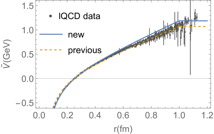
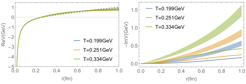
As in Refs. ZhanduoTang:2023tsd , the masses are extracted from the pole positions of spectral functions (imaginary parts of the correlation functions) with point operators which are given by the correlation functions in Eq. (14) but without the wave function . With and GeV2 (compared to 0.27 and 0.225 GeV2, respectively, in our previous work) we indeed find an appreciable improvement in describing the vacuum masses of charmonia and bottomonia as given by recent data from the Particle Data Group (PDG) ParticleDataGroup:2018ovx , while keeping the mixing parameter at =0.8. The masses of almost all states below the open-bottom threshold are now within 20 MeV of the experimental values (with the exception of the ), see Table 1 for the comparison of vacuum bottomonium spectroscopy between -matrix results and experimental data. The new potential slightly deviates from the vacuum free energy obtained from lQCD at large distances (and from our previous version), see Fig. 1. The vacuum charmonium masses show a similar improvement relative to the previous potential.
| Channel | Particle | Exp. |
|
|
|||||||||
|---|---|---|---|---|---|---|---|---|---|---|---|---|---|
| S | 9.859 | 9.862 | 9.870 | ||||||||||
| 10.233 | 10.250 | 10.221 | |||||||||||
| PS | 9.399 | 9.417 | 9.474 | ||||||||||
| V | 9.460 | 9.460 | 9.517 | ||||||||||
| 10.023 | 9.994 | 9.997 | |||||||||||
| 10.355 | 10.370 | 10.339 | |||||||||||
| AV1 | 9.899 | 9.890 | 9.895 | ||||||||||
| AV2 | 9.893 | 9.887 | 9.888 | ||||||||||
| 10.255 | 10.272 | 10.247 | |||||||||||
| T | 9.912 | 9.900 | 9.898 | ||||||||||
| 10.269 | 10.287 | 10.250 |
4 In-Medium Potentials Constrained by lQCD
We now turn to analyzing the lQCD results for the bottomonium correlators with extended operators. As mentioned above, key inputs are the potential as well as the interference functions. Since we want to maintain the consistency with our previous fits to the WLCs, and since the results are embedded into the light-parton sector to maintain a realistic equation of state, our procedure is based on a variational method that involves two iterative loops, as follows: Initially, we refine the in-medium potential using the effective mass () of bottomonum correlators defined in Eq. (18) as well as the effective mass of WLCs, which will be discussed in Sec. 4.2. These quantities, derived from the -matrix approach, are fitted to lQCD data. Using the such adjusted potentials, we proceed to calculate the QGP EoS, modifying the main parameters in this sector, which are the “bare” masses of the in-medium light quarks and gluons. The computation of the EoS involves both one-body spectral functions and two-body scattering amplitudes, requiring the solution of a selfconsistency problem carried out through numerical iteration. Following this, we recompute the HQ self-energies from the heavy-light -matrices and reintegrate these results into the calculations of and using the in-medium quarkonium spectral functions. We continue refining the in-medium potential by refitting the effective masses obtained in the -matrix approach to the corresponding lQCD data. The adjusted potential is then employed to fit the EoS again. This loop is repeated until convergence is achieved.
In the remainder of this section, we discuss our numerical fits of the EoS in Sec. 4.1 and the WLCs in Sec. 4.2, followed by a discussion of the results for the bottomonium correlators with extended operators and a comparison of their spectral functions to those with point operators in Sec. 4.3.
4.1 Equation of State
The equation of state is encoded in the pressure, , of a many-body system as a function of temperature and chemical potential; it is connected to the thermodynamic potential per unit volume via . For interacting quantum systems, the pressure can be computed diagrammatically within the Luttinger-Ward-Baym (LWB) formalism Luttinger:1960ua ; Baym:1961zz ; Baym:1962sx . This includes an interaction contribution represented by the Luttinger-Ward functional (LWF), which constitutes a thermodynamically consistent formalism when combined with the latter resummation in the -matrix. For strongly interacting systems, it is important to resum the fully dressed skeleton diagrams in the LWF, which can be achieved with a matrix-logarithm technique Liu:2016ysz . This enables to account for the contributions from dynamically formed bound states and/or resonances to the EoS. The thermodynamic potential is given by Liu:2016ysz ; Liu:2017qah
| (19) |
where and with . The summation in Eq. (19) includes all light-parton channels characterized by the spin-color degeneracy , with the sign distinguishing bosons () from fermions (). The three components of Eq. (19) , , and correspond to the contributions from quasiparticles, their selfenergies, and two-body interactions (LWF), respectively.
The final converged results are very similar to our previous work in Ref. ZhanduoTang:2023pla : the contribution from the two-body interactions become more significant as the temperature decreases, driven by the formation of bound states in the attractive color channels (singlet and anti-triplet). This indicates a transition in the degrees of freedom within the system from partons to mesons and diquarks at lower temperatures, which is in agreement with the insights of earlier work Liu:2017qah .
4.2 Static Wilson Line Correlators
Next, we turn to the static WLCs in Euclidean time, which are related to the static spectral functions, , via a Laplace transform,
| (20) |
where is the separation between and and their total energy (subtracted by twice bare HQ mass, numerically taken as GeV). The constituent static HQ mass is the sum of the bare mass and the mass shift originating from the self-energy, i.e., Liu:2017qah (the Fock term, , defined below Eq. (4) reduces to in the static limit). In the -matrix formalism, the spectral function takes the following form Liu:2017qah ; ZhanduoTang:2023pla ,
| (21) |
As introduced in Sec. 2 and 2.2, , and in Eq. (21) are the static in-medium potential, two-body selfenergy and interference function, respectively.
The comparison to the lattice data is performed in terms of the effective masses of the WLCs, defined as as Bala:2021fkm . Similar to the correlators with extended operators discussed in Sec. 2.2, the temperature-independent parts at high energies, stemming from excited states related to hybrid potentials, are subtracted from the lattice WLCs. Similar to our previous study ZhanduoTang:2023pla , the WLCs from -matrix show a fair overall agreement with the lQCD results for both the intercept at and the slopes of , although larger discrepancies are observed at the highest temperature. The main reason for this is that the stronger input potential leads to an unstable fitting procedure due to the emergence of glueball condensation, which limits our efforts to improve the fits (see Ref. ZhanduoTang:2023pla for more details).
4.3 Bottomonium Correlators with Extended Operators
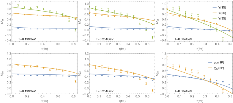
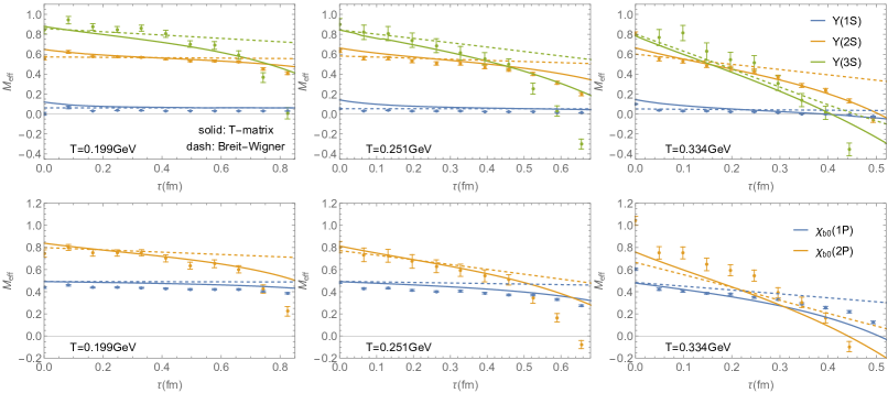
The final results of our fits (which encompass the EoS and WLCs displayed in the previous two sections as well) to the effective masses of bottomonium correlators with extended operators are summarized in Fig. 2 for three temperatures for which lattice data are available Larsen:2019bwy . In performing this comparison one should keep in mind that in lattice-NRQCD calculations one does not obtain the bottomonium masses but energy levels of different bottomonium states, which depend on the details of the lattice-NRQCD formulation. Therefore, in these calculations the energy levels are given with respect to a baseline energy level. In Ref. Larsen:2019zqv the spin-average energy of the 1S bottomonia, , is used as the baseline and the energy levels of other bottomonium states are given with respect to this baseline. Therefore, in the present work we use the spin-average binding energy of 1S bottomonia as reference point for the effective masses. However, this is still not a one-to-one correspondence between the binding energies in -matrix approach and the energy levels of NRQCD. Thus we use a smaller value for the relative shift to perform the comparison with the lattice data: GeV. A fair overall agreement with the lQCD results is achieved for both the intercept at and the slopes of .
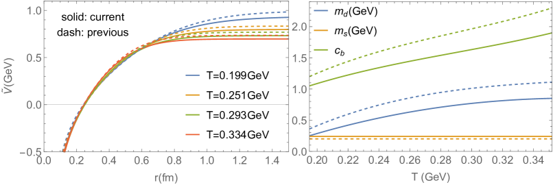
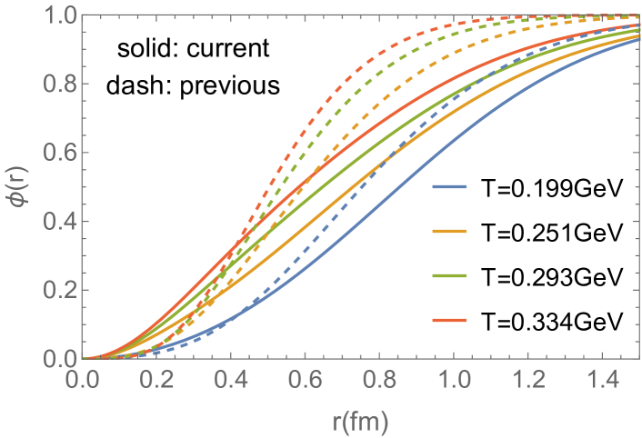
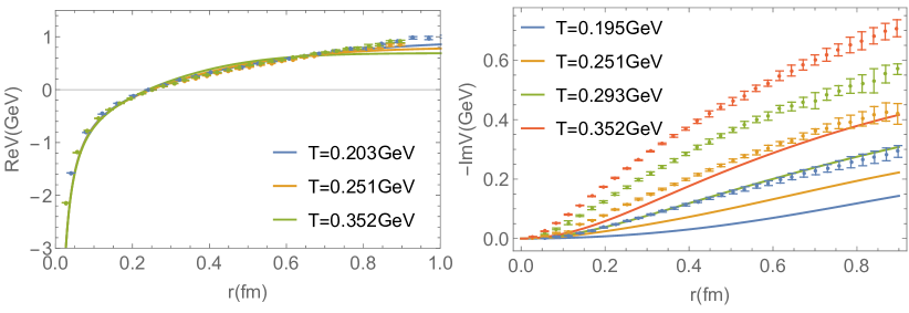
The corresponding in-medium input potentials and their parameters are displayed in Fig. 3. The potentials show essentially no screening for fm, consistent with recent lQCD studies on the energy of static pairs Bala:2021fkm ; Bazavov:2023dci . Compared to our previous studies ZhanduoTang:2023pla where the potentials were only constrained by the QCD EoS and static WLCs, the potentials in this work are a little weaker (more prominent for =0.199GeV) at large distances (the reduction of confining potential due to a larger outweighs its enhancement due to a larger ) but more attractive at small distances (due to the enhancement of the Coulomb potential with a smaller and larger ); however, the differences between these two studies are rather modest. More significant changes take place in the interference functions, as shown in Fig. 4. The interference effects become overall more pronounced (smaller values of the functions), which indicates weakening of the coupling of the color-singlet state to the medium partons.
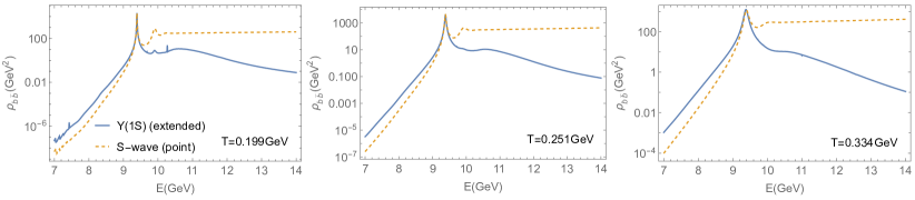
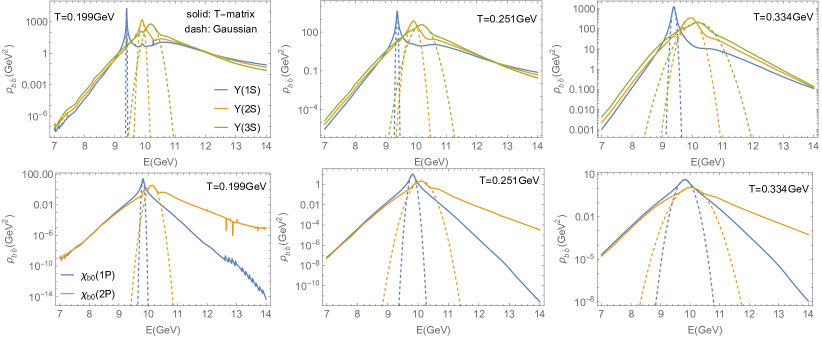
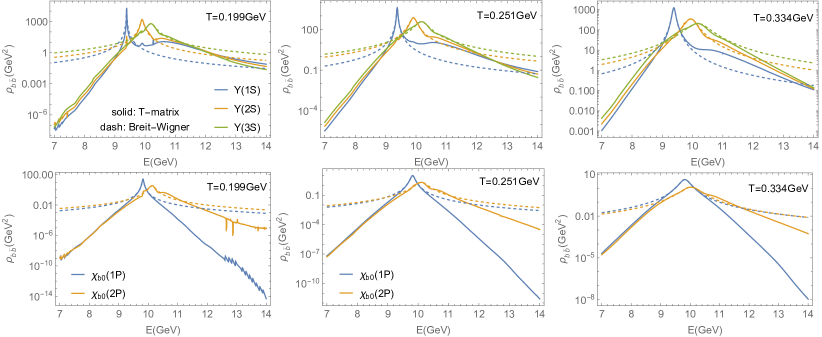
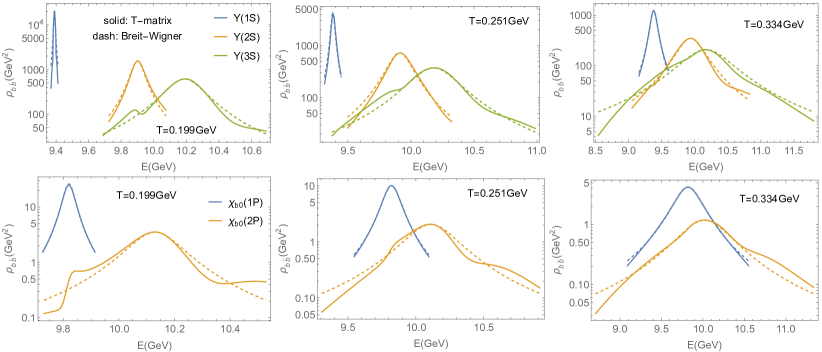
To scrutinize and interpret the bound-state properties underlying our calculations, we compare the bottomonium spectral functions with extended and point operators (without wave functions, , in Eq. (14)) in Fig. 5. For the state, the spectral functions corresponding to both type of meson operators agree well with each other up to the highest considered temperature of 334 MeV. In the case of extended operators the and spectral functions show the presence of peak structures up to MeV. However, as the temperature increases these structures become quite broad and visibly non-symmetric for higher lying bottomonium states. In fact, the width of these peaks is comparable or even larger than the mass difference of various bottomonium states. Therefore, the interpretation of these peaks in terms of bound states is questionable. The -wave spectral functions corresponding to point meson operators convey a different message. The state can be seen at MeV, but it is difficult to identify this state at higher temperature. Furthermore, no structures that can be associated with can be identified in the spectral function corresponding to the point meson operators. This may imply that is melted at temperatures between 200 MeV and 250 MeV.
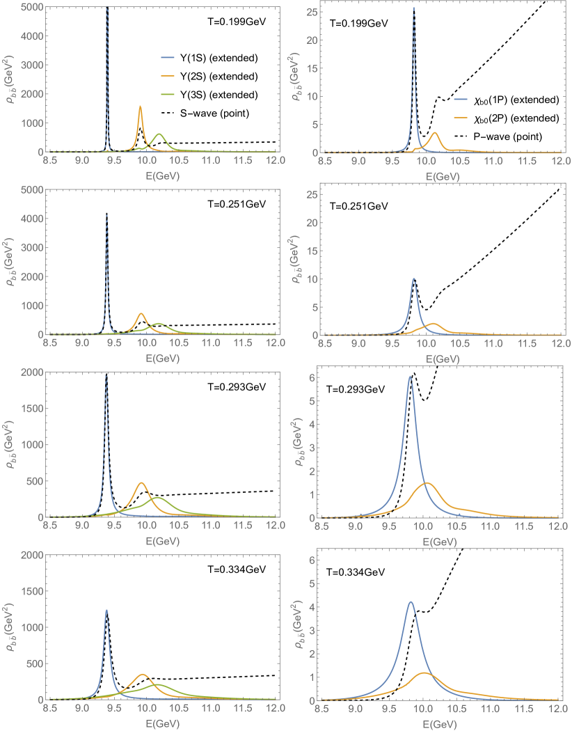
The and spectral functions corresponding to the extended meson operators show peak structures for all temperatures up to MeV. The peak corresponding to state is quite broad and visibly asymmetric already at MeV. As the temperature increases the width of this peak increases significantly. The peak corresponding to state also broadens with increasing temperature. At the highest two temperatures the width of both and bottomonia is comparable or larger that the energy difference between these two states. In the -wave spectral functions corresponding to point operators we can identify the state for MeV and MeV, but no such states can be identified at the highest two temperatures shown in Fig. 5. However, we do not see the peak corresponding to the state at any temperature. Thus, the analysis suggests that the bottomonium state melts around a temperature of MeV. We note that whenever well defined peaks exist in the spectral functions of point meson operators, the corresponding peak position agrees with the one in the spectral function of extended meson operators. Therefore, these peak positions can be interpreted as in-medium bottomonium masses.
To further assess the disappearance of a bound state we resort to a method employed in Ref. Cabrera:2006wh which relies on identifying the poles in the -matrix. Toward this end we write the solution of the -matrix equation in operator form as
| (22) |
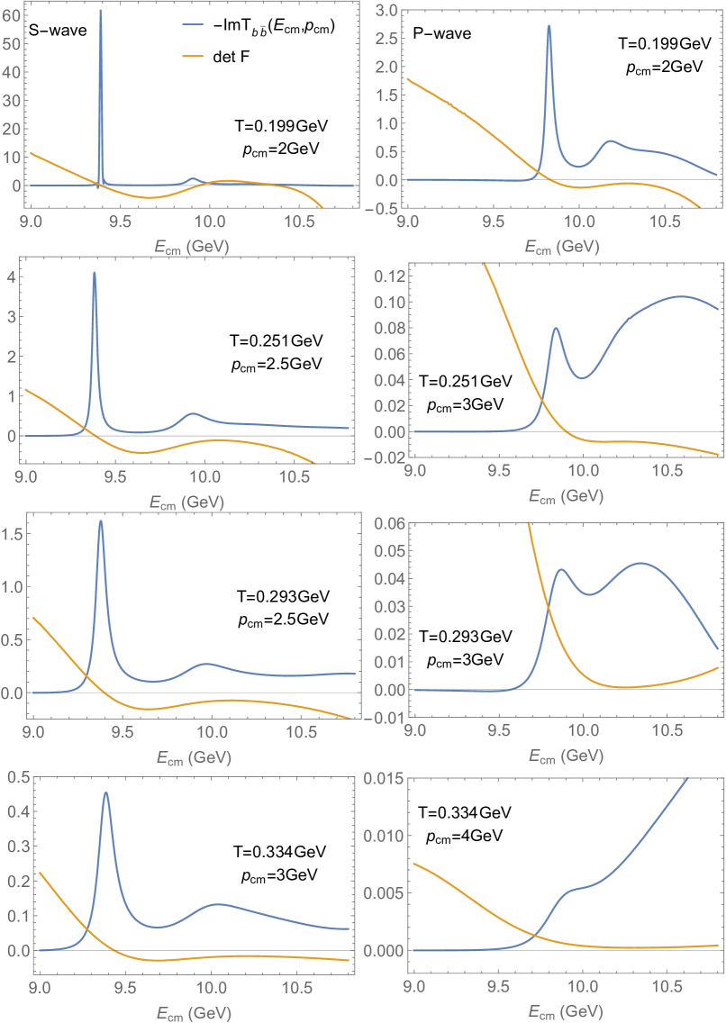
(in practice, this corresponds to discretizing the momentum integral with , and Haftel:1970zz ). Defining , the requirement (for ) indicates the presence of a bound state. This is so because a bound state is characterized by a pole of the scattering amplitude on the real energy axis below the threshold energy, (this corresponds to identifying the zeros of the Jost function in -matrix theory). We depict as a function of total energy at various temperatures, together with the imaginary parts of the -matrices in Fig. 6. As discussed in Sec. 2.2, the -matrices with interference effect are not positive-definite at low momenta, thus we display them at somewhat larger momenta in Fig. 6 to show the peaks corresponding to the bound states more clearly. We have found that the peak locations in the -matrix are not sensitive to this choice and in any case are only shown for guidance; the Jost function, as a determinant in momentum space, does not depend on momentum.
For the -wave results at 199 MeV, crosses zero three times, but only the first two ( and ) are accompanied by identifiable peaks in the imaginary part and can be regarded as bound states, the energy for third zero-crossing (GeV) is already above the threshold (GeV). Only for temperatures MeV we have a zero crossing below the threshold that can be identified with the state. At the next higher temperature, =251 MeV, the pole has also disappeared even though a peak with a width comparable or larger than the binding energy still shows up in the imaginary part of the -matrix which is very similar to the pertinent point spectral function. We still have a pole corresponding to the state at temperatures around 220 MeV, so its “dissociation” temperature is slightly higher than this. The state, on the other hand, still persists at the highest temperature considered in this study. In the -wave channel we see a zero corresponding to state at =251ṀeV, but this zero is about to disappears at =293 MeV. On the other hand, the zero corresponding to state disappears close to 174 MeV.
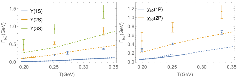
To better understand the physical meaning of different structures in the spectral function and to facilitate the comparison with the lattice results it is useful to quantify the width of these structures by extracting the full width at half maximum (FWHM). For spectral functions corresponding to the point operators such this definition cannot always be executed since the right side of the peak merges with the continuum for high temperatures. The widths for different states obtained from the spectral functions of extended meson operators are shown in Fig. 7 as a function of temperature either as solid lines or dashed lines, where the latter continue beyond the “dissociation” temperature (i.e., where the poles on the real axis cease to exist). The widths obtained from the spectral functions with point meson operators are displayed as dashed-dotted lines up to a temperature where the FWHM can be defined. We find reasonably good agreement between the results from the spectral functions corresponding to extended operators and the ones from point operators. In Fig. 7 we also display the width parameter obtained in lattice calculations using a Gaussian parametrization of the peak of the spectral function Larsen:2019zqv ; Larsen:2019bwy . The FWHM is related to the Gaussian width parameter as FWHM, which We take into account when comparing the -matrix and lattice results for the width in Fig. 7. The widths of different bottomonia states extracted from the fits in Refs. Larsen:2019zqv ; Larsen:2019bwy are larger than the ones obtained in the -matrix calculations. The main reason for this difference is the use of simple Gaussian form of the spectral function in Refs. Larsen:2019zqv ; Larsen:2019bwy . For a Gaussian form of the spectral function the dependence of the effective masses is entirely determined by , because the energy region far away from the peak does not contribute to the correlator, while for realistic spectral shapes the behavior of the spectral function far away from the peak position is important for the -dependence of the effective masses. This is discussed in Appendix B, where we also show that a cut Lorentzian form of the spectral function with a width parameter , i.e., a form where the spectral function is given by a Lorentzian (Brei-Wigner) in the interval with representing the peak position and is zero otherwise, provides a better parametrization of the spectral function from the lattice studies.
We thus conclude that the results from spectral functions with extended operators have to be interpreted with care. While for tightly bound states the results are in agreement for both the peak mass and widths with the point spectral functions, this is no longer the case for the excited states. The extended operator results still produce peaks which however are not a reliable indication of a bound state. On the other hand, the “masses” and “widths” of these “pseudo-peaks” can still provide information on the underlying potential and inelastic scattering rates of the heavy quarks at the distance probed by the optimized wave function. Furthermore, using a Gaussian form of the spectral function when fitting the lattice results on the correlation function tends to overestimate the in-medium bottomonium width appreciably.
5 Heavy-Quark Transport Coefficients
In this section, we utilize our newly constrained potential to predict HQ transport coefficients in the QGP. The main ingredients to the charm-quark transport coefficients are the heavy-light scattering amplitudes and parton spectral functions. Similar to our previous study ZhanduoTang:2023pla , the parton spectral functions show strongly broadened peaks and collective modes on the low-energy shoulder of the quasiparticle peaks at zero parton momentum, even at high temperatures (which is different from the HQ free energy-based results Liu:2017qah where the interaction strength is more strongly screened at high temperatures). Another feature is that the parton widths do not fall off with 3-momentum as much as the ones from earlier potentials which focused on fitting the in-medium HQ free energies; this is mainly due to the vector admixture to the confining interaction which generates relativistic (magnetic) corrections at large momenta (recall that a mixing coefficient of has been used as introduced in Sec. 3). For the heavy-light scattering amplitudes, it is crucial to account for the broad spectral functions in the evaluation of the HQ transport coefficient Liu:2018syc , which enables to access the sub-threshold interaction strength generated by dynamically formed -meson bound states at relatively low temperatures. Again, when comparing to the HQ free energy-based results Liu:2017qah , we find a harder momentum dependence of the scattering amplitudes as well as larger scattering amplitudes at high temperatures. However, our results do not differ much from those in Ref. ZhanduoTang:2023pla where the in-medium potentials have been constrained by static WLCs and QGP EoS but not by the bottomonium correlators with extended operators. This indicates that the systematic application of lQCD constraints stabilizes in terms of the underlying potentials and resulting transport properties of the QGP.
The HQ friction coefficient (relaxation rate) with off-shell spectral functions can be evaluated based on the Kadanoff-Baym equations as Liu:2018syc
| (23) | ||||
Here, denotes the energy-momentum conserving -function and the spin-color degeneracy of charm quarks. The summation, , is over all light quarks and gluons in the heat bath. The friction coefficient is evaluated for a definite energy and moment of the incoming charm quark, whereas all other partons are represented by off-shell spectral functions. The heavy-light scattering amplitudes, , are related to the -matrices and incorporate the summation over all possible two-body color and partial-wave channels as detailed in Ref. Liu:2018syc .
Compared to our previous study ZhanduoTang:2023pla , where the in-medium potentials were constrained by the static WLCs and the QGP EoS only, the charm-quark friction coefficient is slightly larger at =251, 293 and 334 MeV, while at =199 MeV the results are comparable in both scenarios. At low momenta, there is some compensation between the smaller charm-quark masses in the present work, which enhances (recall that the relaxation rate is proportional to the temperature-over-mass ratio), the stronger potential but also a stronger screening of the confining force (=240 MeV compared to 200 MeV before). At high momenta, where the short-range color-Coulomb interaction is dominant (further augmented by relativistic corrections), its weaker screening, especially at higher temperatures, implies that the in this work is significantly larger than in the previous one.
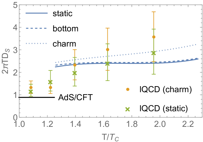
The spatial diffusion coefficient, , scaled by the inverse thermal wavelength, , is displayed in Fig. 8 as a function of temperature. Our results are in fair agreement with recent lQCD data Altenkort:2023oms ; Altenkort:2023eav for charm and static quarks. The result for static quark is about a factor of 2-3 larger than the result from the AdS/CFT correspondence which is believed to provide a quantum lower bound for the diffusion coefficient Casalderrey-Solana:2006fio . Our results are comparable with those in previous study (WLC-based) ZhanduoTang:2023pla , although our is slightly higher at the lowest temperature due to a weaker confining interaction.
6 Conclusions
We have employed the thermodynamic -matrix approach to study bottomonium correlators with extended operators, as recently computed in lattice QCD. Starting from a slightly amended vacuum potential (with larger coupling constant and string tension) which improves the bottomonium spectroscopy in vacuum, medium modifications have been constrained by the QGP equation of state, static Wilson line correlators and bottomonium correlators with extended operators from lQCD using selfconsistent -matrix solutions. A fair agreement with lQCD data could be achieved for the effective masses of - and -wave bottomonia from the correlators with extended operators. The spectral functions in the -matrix approach with extended operators show peaks for all bottomonium states in the entire temperature region considered, even though some of these peaks are very broad and asymmetric. The -wave and -wave spectral functions of point meson operators from the -matrix approach feature a disappearance of the excited bottomonium states at certain temperatures. Therefore, not all peak structures in the spectral functions of extended operators can be interpreted as bound states, and the effective width obtained in lattice QCD calculations in Refs. Larsen:2019bwy ; Larsen:2019zqv cannot be always interpreted as an in-medium width (or reaction rate). Using the poles of the -matrix on the real energy axis using Jost functions we assessed “dissociation” temperatures of , , and bottomonium states to be and MeV, respectively. For bottomonium state this temperature is larger than 334 MeV. Well below the dissociation temperatures, the in-medium masses, determined as the peak position of the spectral functions of extended or point operators or as the real-axis pole of the T-matrix agree with each other reasonably well. Furthermore, the in-medium widths obtained from the spectral functions of point and extended operators also agree below the “dissociation” temperatures. This implies that while the spectral functions of extended meson operators cannot be used to study the dissociation of different bottomonium states, they are still suitable to study in-medium bottomonium properties for smaller temperatures. We also note that the effective width obtained in the -matrix approach with extended meson operators is smaller than the one obtained in lattice QCD calculations Larsen:2019bwy ; Larsen:2019zqv . This is in large part due to the use of a simple Gaussian form of the spectral function, which does not capture the low-energy tails found in the microscopic calculations of the quantum many-body approach. A more realistic form such as a Lorentzian, the spectral function in the lattice analysis would yield smaller in-medium bottomonium width, although energy cutoffs are required to mimic the energy dependent selfenergies as generated by microscopic calculations.
The inferred in-medium potentials are quite similar to those in our previous study where they have been constrained by the QGP EoS and static WLCs only, but the interference effects turn out to be more significant when also including the constraints from correlators with extended operators. The main features for the spectral and transport properties from our previous and current studies remain intact: significant low-energy collective modes for parton spectral functions at high temperatures, resonant structures in the heavy-light scattering amplitudes, and a weak temperature dependence of the predicted spatial diffusion coefficient in fair agreement with recent 2+1-flavor lQCD results. The thermal relaxation rate (friction coefficient) in the present work is slightly larger at higher temperatures but closely agrees with our previous study at lower ones. Ongoing work is directed at implementing these transport coefficients into phenomenological applications in heavy-ion collisions, to evaluate the impact on, and theoretical uncertainty in, describing the open HF observables. This is, in fact, part of a larger effort to utilize the nonperturbative -matrices also in the quarkonium sector, e.g., to calculate their inelastic reaction rates and the pertinent (quantum) kinetics of heavy quarkonia in an evolving QCD medium.
Acknowledgements.
This work has been supported by the U.S. National Science Foundation under grant no. PHY-2209335, by the U.S. Department of Energy, Office of Science, Office of Nuclear Physics through contract No. DE-SC0012704 and the Topical Collaboration in Nuclear Theory on Heavy-Flavor Theory (HEFTY) for QCD Matter under award no. DE-SC0023547. We thank Hai-Tao Shu and Rasmus Larsen for helpful discussions.Appendix A Spectral Representation for Quarkonium Correlators with Extended Operators
In this section, we derive the spectral representation for the quarkonium correlators with extended operators following Refs. Karsch:2000gi ; Aarts:2005hg ; Alberico:2004we . The summation in Eq. (8) becomes an integration in the continuum limit:
| (24) |
where is the lattice volume. The correlator introduced in Sec. 2.2 is connected to its frequency-momentum-space components by a Fourier transform
| (25) |
where is the total momentum of bottomonium and is usually set to . Defining the bottomonium spectral functions as
| (26) |
the correlators can be expressed in a mixed representation through the spectral functions as
| (27) |
To obtain the correlators, , required for evaluating the effective mass in Eq. (18), one has to first find through the inverse transform of Eq. (25):
| (28) |
and then plug it into Eq. (26) to get the spectral functions. Finally, the correlators, , can be computed via Eq. (27).
The correlation function, consists of two components, i.e., the free part, , and the interacting part, , which can be evaluated directly from the definition introduced in Sec. 2.2. For the free contribution, one has
| (29) | ||||
where is the quark propagator Alberico:2004we . Then, the correlators in space are given by
| (30) | ||||
where the Fourier transforms, and , have been applied in the second equality, and in the fourth equality. In the fifth equality of Eq. (30), we have used the fact that the Matsubara frequencies for mesons and quarks are and , respectively. A positive-energy projected propagator has been used in the sixth equality: is the two-body propagator introduced in Eq. (2), and are the positive/negative energy projectors Cabrera:2006wh ; Riek:2010fk ; ZhanduoTang:2023tsd for quark () and antiquark (), respectively.
The interacting part of correlators is given by:
| (31) | ||||
where is the point operator, and denotes the 2-body scattering amplitude. Applying similar techniques as used in Eq. (30), the correlators in space are given by
| (32) | ||||
Combining Eq. (30) and Eq. (32) gives Eq. (14) (recall that the total momentum is usually set to ). The overall factor is canceled out in the ratio used to define the effective mass, see Eq. (18). The derivation presented above, which uses non-optimized operators, can be readily extended to the one with optimized operators, given that the latter are simply linear combinations of the former as discussed in Sec. 2.2.
Appendix B Spectral Functions for Point- and Extended-Meson Operators
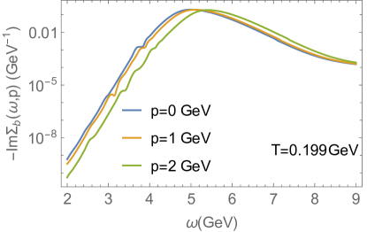
In this appendix we discuss some details of the determination of the thermal widths from the spectral functions for point and extended meson operators and the comparison with the lattice QCD results. In Fig. 9 we show the bottomonium spectral function of states calculated with point and extended meson operators using logarithmic scale on the -axis. We see that for energies, , well below the peak position the spectral function decays exponentially for both type of meson operators. This exponential decrease is related to the exponential decrease of the imaginary part of the in-medium -quark selfenergy at small energies, as shown in Fig. 10 for =199 MeV as an example. In the case of point operators the spectral function does not decrease with increasing for energies well above the peak. For extended meson operators the spectral function decreases with increasing for sufficiently large values, but we see a prominent shoulder structure above the peak, which leads to significant increase in the effective mass at small .
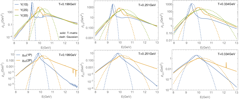
In Fig. 11 we show the spectral function corresponding to the extended-meson operators for , , , and states. We see that for all states the spectral function decays exponentially far away from the peak at about the same rate, although there is a shoulder structure visible for the and spectral functions. It is instructive to compare the obtained spectral function with a simple Gaussian parametrization,
| (33) |
with a Gaussian parameter determined from the FWHM (see main text), and being the in-medium bottomonium mass. This parametrization is also shown in Fig. 11 as dashed lines. While in the vicinity of the peak the Gaussian parametrization describes the spectral function fairly well, it is very different away from the peak, i.e., it is much smaller than the spectral function from the -matrix calculations. In Fig. 12 we compare our spectral functions corresponding to extended meson operators for different states with the Gaussian parametrization used in Ref. Larsen:2019zqv . We see that the Gaussian parametrization used in the lattice study gives much broader peaks. This is because in order to describe the dependence of the lattice bottomonium correlators and compensate for the rapid fall-off of the Gaussian a larger width is needed.
Next we compare our spectral function with the Breit-Wigner (Lorentzian) parametrization,
| (34) |
with being the FWHM and the in-medium mass of the bottomonium state.
In Figs. 13 and 14 we compare this parametrization with the spectral function obtained from the -matrix calculations. We see that in the interval the Breit-Wigner form provides a good description of the full spectral function corresponding to the extended meson operators of , and states, and a fair description of the full spectral function corresponding to and states. The Laplace transform of the Lorentzian form does not exist because the corresponding integrand does not vanish exponentially for small . For this reason a Lorentzian form cannot be used to model the lattice QCD results, and a Gaussian form was used. However, if we introduce a cutoff into the Lorentzian spectral function, i.e., a Lorentzian in the interval and zero otherwise, then the Laplace transform can be performed. In Fig. 15 we show the effective masses obtained from such a form of the spectral function and compare them to the effective masses obtained from the -matrix spectral function and the effective masses from lattice NRQCD calculations Larsen:2019zqv . We see that at small the effective masses obtained from the cut Lorentzian form are very similar to the effective mass obtained with the -matrix spectral function. There are difference in the effective masses at larger . However, even the -matrix spectral function cannot fully describe the lattice QCD results on the effective masses at large . This is due to an additional contribution to the bottomonium spectral function at very low energy specific to NRQCD Bala:2021fkm , which is unrelated to the bound state peak. Such a contribution is not present in -matrix approach or in lattice QCD calculations with relativistic heavy quarks. Thus a cut Lorentzian form provides a reasonable parametrization of the spectral function that can be used in lattice QCD analysis. Using such parametrization for fitting the effective masses would result in significantly smaller width parameters, , and the difference between the lattice and -matrix results in Fig. 7 is understood as being due to using an unrealistic form of the spectral function in Ref. Larsen:2019zqv .
Appendix C Potential Comparisons to Existing Work
In this appendix, we compare both the real and imaginary parts of the static potential from our work to the findings of other studies in the literature. Recall that the real part is the screened Cornell potential, given by Eq. (5), with parameters shown in Fig. 3. The imaginary part of the potential in our study is expressed as (see Eq.(15)), where represents the 2-body selfenergy, and the interference function is shown by the solid lines in Fig. 4.
We compare our potential to that in Ref. Bazavov:2023dci , which has been extracted from lQCD data on WLCs using a Lorentzian spectral function with energy cutoff, as shown in Fig. 16, and to Ref. Shi:2021qri where it has been is fitted to lQCD results of bottomonium thermal widths using a Gaussian ansatz applied via deep neural networks. The real part of the potential in our study shows reasonable agreement with those presented in both Refs. Bazavov:2023dci and Shi:2021qri . However, there is a notable difference in the imaginary part: in our study, it is approximately 2 to 3 times smaller than for the Lorentzian- and Gaussian-based fits at large distances, with even more significant differences at short distances. This observation aligns qualitatively with the findings in Appendix B: to describe the same lQCD data for bottomonium effective masses with extended operators, the Gaussian fit requires a much larger width than that obtained from the microscopic -matrix calculations, as shown in Fig. 12. Similarly, although the width required by the cut Lorentzian fit is smaller than that of the Gaussian fit, it remains larger than the width from the -matrix. As indicated in Fig. 15, the Lorentzian fit with cutoff still requires a larger width to achieve the necessary slope in for reproducing the lattice data. The comparison for the imaginary part of the potential can probably be made more consistent if a more realistic spectral function were used in the lattice study.
References
- (1) Francesco Prino and Ralf Rapp. Open Heavy Flavor in QCD Matter and in Nuclear Collisions. J. Phys. G, 43(9):093002, 2016.
- (2) Xin Dong and Vincenzo Greco. Heavy quark production and properties of Quark–Gluon Plasma. Prog. Part. Nucl. Phys., 104:97–141, 2019.
- (3) R. Rapp, D. Blaschke, and P. Crochet. Charmonium and bottomonium production in heavy-ion collisions. Prog. Part. Nucl. Phys., 65:209–266, 2010.
- (4) Louis Kluberg and Helmut Satz. Color Deconfinement and Charmonium Production in Nuclear Collisions. 2010.
- (5) P. Braun-Munzinger and J. Stachel. Charmonium from Statistical Hadronization of Heavy Quarks – a Probe for Deconfinement in the Quark-Gluon Plasma. Landolt-Bornstein, 23:424, 2010.
- (6) A. Andronic et al. Comparative study of quarkonium transport in hot QCD matter. Eur. Phys. J. A, 60(4):88, 2024.
- (7) G. Aarts, C. Allton, S. Kim, M. P. Lombardo, S. M. Ryan, and J. I. Skullerud. Melting of P wave bottomonium states in the quark-gluon plasma from lattice NRQCD. JHEP, 12:064, 2013.
- (8) Gert Aarts, Chris Allton, Tim Harris, Seyong Kim, Maria Paola Lombardo, Sinéad M. Ryan, and Jon-Ivar Skullerud. The bottomonium spectrum at finite temperature from Nf = 2 + 1 lattice QCD. JHEP, 07:097, 2014.
- (9) Seyong Kim, Peter Petreczky, and Alexander Rothkopf. Lattice NRQCD study of S- and P-wave bottomonium states in a thermal medium with light flavors. Phys. Rev. D, 91:054511, 2015.
- (10) Rasmus Larsen, Stefan Meinel, Swagato Mukherjee, and Peter Petreczky. Thermal broadening of bottomonia: Lattice nonrelativistic QCD with extended operators. Phys. Rev. D, 100(7):074506, 2019.
- (11) Rasmus Larsen, Stefan Meinel, Swagato Mukherjee, and Peter Petreczky. Excited bottomonia in quark-gluon plasma from lattice QCD. Phys. Lett. B, 800:135119, 2020.
- (12) Rasmus Larsen, Stefan Meinel, Swagato Mukherjee, and Peter Petreczky. Bethe-Salpeter amplitudes of Upsilons. Phys. Rev. D, 102:114508, 2020.
- (13) Agnes Mocsy, Peter Petreczky, and Michael Strickland. Quarkonia in the Quark Gluon Plasma. Int. J. Mod. Phys. A, 28:1340012, 2013.
- (14) E. Megias, E. Ruiz Arriola, and L. L. Salcedo. Dimension two condensates and the Polyakov loop above the deconfinement phase transition. JHEP, 01:073, 2006.
- (15) M. Mannarelli and R. Rapp. Hadronic modes and quark properties in the quark-gluon plasma. Phys. Rev. C, 72:064905, 2005.
- (16) Felix Riek and Ralf Rapp. Selfconsistent Evaluation of Charm and Charmonium in the Quark-Gluon Plasma. New J. Phys., 13:045007, 2011.
- (17) Shuai Y. F. Liu and Ralf Rapp. -matrix Approach to Quark-Gluon Plasma. Phys. Rev. C, 97(3):034918, 2018.
- (18) Zhanduo Tang and Ralf Rapp. Spin-dependent interactions and heavy-quark transport in the quark-gluon plasma. Phys. Rev. C, 108(4):044906, 2023.
- (19) Zhanduo Tang, Swagato Mukherjee, Peter Petreczky, and Ralf Rapp. T-matrix analysis of static Wilson line correlators from lattice QCD at finite temperature. Eur. Phys. J. A, 60(4):92, 2024.
- (20) D. Cabrera and R. Rapp. T-Matrix Approach to Quarkonium Correlation Functions in the QGP. Phys. Rev. D, 76:114506, 2007.
- (21) F. Riek and R. Rapp. Quarkonia and Heavy-Quark Relaxation Times in the Quark-Gluon Plasma. Phys. Rev. C, 82:035201, 2010.
- (22) R. Brockmann and R. Machleidt. The Dirac-Brueckner Approach. Int. Rev. Nucl. Phys., 8:121–169, 1999.
- (23) Adam P. Szczepaniak and Eric S. Swanson. On the Dirac structure of confinement. Phys. Rev. D, 55:3987–3993, 1997.
- (24) N. Brambilla and A. Vairo. Nonperturbative dynamics of the heavy - light quark system in the nonrecoil limit. Phys. Lett. B, 407:167–173, 1997.
- (25) D. Ebert, R. N. Faustov, and V. O. Galkin. Properties of heavy quarkonia and mesons in the relativistic quark model. Phys. Rev. D, 67:014027, 2003.
- (26) V. D. Mur, V. S. Popov, Yu. A. Simonov, and V. P. Yurov. Description of relativistic heavy - light quark - anti-quark systems via Dirac equation. J. Exp. Theor. Phys., 78:1–14, 1994.
- (27) W. Lucha, F. F. Schoberl, and D. Gromes. Bound states of quarks. Phys. Rept., 200:127–240, 1991.
- (28) M. Tanabashi et al. Review of Particle Physics. Phys. Rev. D, 98(3):030001, 2018.
- (29) Luis Altenkort, Olaf Kaczmarek, Rasmus Larsen, Swagato Mukherjee, Peter Petreczky, Hai-Tao Shu, and Simon Stendebach. Heavy Quark Diffusion from 2+1 Flavor Lattice QCD with 320 MeV Pion Mass. Phys. Rev. Lett., 130(23):231902, 2023.
- (30) Luis Altenkort, David de la Cruz, Olaf Kaczmarek, Rasmus Larsen, Guy D. Moore, Swagato Mukherjee, Peter Petreczky, Hai-Tao Shu, and Simon Stendebach. Quark Mass Dependence of Heavy Quark Diffusion Coefficient from Lattice QCD. Phys. Rev. Lett., 132(5):051902, 2024.
- (31) M. Laine, O. Philipsen, P. Romatschke, and M. Tassler. Real-time static potential in hot QCD. JHEP, 03:054, 2007.
- (32) Gyan Bhanot and Michael E. Peskin. Short Distance Analysis for Heavy Quark Systems. 2. Applications. Nucl. Phys. B, 156:391–416, 1979.
- (33) Taesoo Song and Su Houng Lee. Quarkonium-hadron interactions in perturbative QCD. Phys. Rev. D, 72:034002, 2005.
- (34) A. Bazavov et al. Equation of state in ( 2+1 )-flavor QCD. Phys. Rev. D, 90:094503, 2014.
- (35) J. M. Luttinger and John Clive Ward. Ground state energy of a many fermion system. 2. Phys. Rev., 118:1417–1427, 1960.
- (36) Gordon Baym and Leo P. Kadanoff. Conservation Laws and Correlation Functions. Phys. Rev., 124:287–299, 1961.
- (37) Gordon Baym. Selfconsistent approximation in many body systems. Phys. Rev., 127:1391–1401, 1962.
- (38) Shuai Y. F. Liu and Ralf Rapp. Spectral and transport properties of quark–gluon plasma in a nonperturbative approach. Eur. Phys. J. A, 56(2):44, 2020.
- (39) Dibyendu Bala, Olaf Kaczmarek, Rasmus Larsen, Swagato Mukherjee, Gaurang Parkar, Peter Petreczky, Alexander Rothkopf, and Johannes Heinrich Weber. Static quark-antiquark interactions at nonzero temperature from lattice QCD. Phys. Rev. D, 105(5):054513, 2022.
- (40) Alexei Bazavov, Daniel Hoying, Rasmus N. Larsen, Swagato Mukherjee, Peter Petreczky, Alexander Rothkopf, and Johannes Heinrich Weber. Unscreened forces in the quark-gluon plasma? Phys. Rev. D, 109(7):074504, 2024.
- (41) Michael I. Haftel and Frank Tabakin. NUCLEAR SATURATION AND THE SMOOTHNESS OF NUCLEON-NUCLEON POTENTIALS. Nucl. Phys. A, 158:1–42, 1970.
- (42) Shuai Y. F. Liu, Min He, and Ralf Rapp. Probing the in-Medium QCD Force by Open Heavy-Flavor Observables. Phys. Rev. C, 99(5):055201, 2019.
- (43) Jorge Casalderrey-Solana and Derek Teaney. Heavy quark diffusion in strongly coupled N=4 Yang-Mills. Phys. Rev. D, 74:085012, 2006.
- (44) F. Karsch, M. G. Mustafa, and M. H. Thoma. Finite temperature meson correlation functions in HTL approximation. Phys. Lett. B, 497:249–258, 2001.
- (45) Gert Aarts and Jose M. Martinez Resco. Continuum and lattice meson spectral functions at nonzero momentum and high temperature. Nucl. Phys. B, 726:93–108, 2005.
- (46) W. M. Alberico, A. Beraudo, and A. Molinari. Meson correlation functions in a QCD plasma. Nucl. Phys. A, 750:359–390, 2005.
- (47) Shuzhe Shi, Kai Zhou, Jiaxing Zhao, Swagato Mukherjee, and Pengfei Zhuang. Heavy quark potential in the quark-gluon plasma: Deep neural network meets lattice quantum chromodynamics. Phys. Rev. D, 105(1):014017, 2022.