Neural Graph Simulator for Complex Systems
Abstract
Numerical simulation is a predominant tool for studying the dynamics in complex systems, but large-scale simulations are often intractable due to computational limitations. Here, we introduce the Neural Graph Simulator (NGS) for simulating time-invariant autonomous systems on graphs. Utilizing a graph neural network, the NGS provides a unified framework to simulate diverse dynamical systems with varying topologies and sizes without constraints on evaluation times through its non-uniform time step and autoregressive approach. The NGS offers significant advantages over numerical solvers by not requiring prior knowledge of governing equations and effectively handling noisy or missing data with a robust training scheme. It demonstrates superior computational efficiency over conventional methods, improving performance by over times in stiff problems. Furthermore, it is applied to real traffic data, forecasting traffic flow with state-of-the-art accuracy. The versatility of the NGS extends beyond the presented cases, offering numerous potential avenues for enhancement.
Dynamics in graphs are pervasive in the world, from packet flow in communication networks [1, 2] and electric current in power grids [3, 4, 5] to the spread of epidemics or rumors [6, 7, 8, 9]. Such dynamics are often modeled using governing equations in the form of differential equations, which are typically analytically intractable due to the intricate topology of complex networks. Consequently, numerical simulations are essential, but these solvers demand significant computational resources, especially for stiff problems [10, 11].
Artificial intelligence (AI) solvers have emerged as a promising approach to address these computational challenges. The prototype of an AI solver, which optimizes neural networks to map spatial and temporal domains to a solution function, was first proposed in 1998 [12]. With the advent of deep learning, this concept evolved into the physics-informed neural networks [13, 14], capable of quickly obtaining solutions at arbitrary locations and times. The surrogate model was successfully applied to various physical systems, including fluid simulations [15]. However, they struggle with complex systems defined on graphs due to the discrete nature of the underlying space. Furthermore, these models are limited when the exact governing equation cannot be established, as with the traditional numerical solvers such as the Runge-Kutta method [16, 17].
When only observational data is accessible without prior knowledge of the system, recurrent neural networks (RNNs) and their variants including long short-term memory (LSTM) and gated recurrent unit (GRU) can be used for simulation. The broad applicability and noise robustness of the RNN have been explored in various dynamical systems, such as Lorenz attractor, generalized Vicsek model, and streamflow system [18]. NeuralODE, combining continuous-depth RNNs and numerical solvers, has successfully reproduced bi-directional spiral simulation [19]. Among the variations of RNNs, reservoir computing (RC), which uses a reservoir as the RNN unit, accurately predicts chaos using simple computation and optimization [20, 21, 22, 23, 24, 25]. Despite its comprehensive study of chaotic complex systems, its implementation in real-world simulations is not practical. The model can only be applied to a specific system instance and cannot be generalized to different conditions.
Graph neural networks (GNNs) [26, 27] are widely used in complex systems due to their natural applicability to graphs. GNNs can handle varying topologies and sizes [28, 29], which is a distinguishing feature to previous neural network architectures. Spatial-temporal GNNs, which use GNN as a recurrent unit, are developed to learn and predict multivariate time series defined on a graph, including traffic forecasting [30]. As an alternative approach, graph network-based simulator [31] performs complex physical simulations, including fluid dynamics. It tracks the changes of interaction pairs between particles in the system every time, creating temporal graphs in which the GNN is applied. However, these approaches share the same constraints with RNNs, requiring the train data to have uniform time intervals and are limited to discrete-time predictions.
Neural operator [32, 33] addresses continuous-time solutions for partial differential equations (PDEs). In this approach, the neural network is trained to approximate an operator that maps the sensor or source function to the solution function in a data-driven manner. Extending this to graphs, a graph kernel network solves second-order elliptic PDE by discretizing the Euclidean space into a proximity graph [34]. However, these approaches predominantly consider regular graphs with approximately constant node degrees, leaving their applications to heterogeneous nodes and generalizations over different graph sizes and topologies unexplored.
In the data-driven approaches, incomplete data, such as noise or missing values, complicates the understanding and simulation of the system. To mitigate the noise, a noise-robust training scheme is proposed, which forces neural networks to simultaneously learn the noise and true trajectory from given incomplete data [35]. Alternatively, the RC is carefully designed to reconstruct the trajectories of the Lorenz and Rössler system with high-intensity Lévy noise [36]. It has also been proposed that the deliberate introduction of noise to the precise data may stabilize the training and prediction of the RC [37]. For the partially observable system, various techniques are employed to fill the missing values. Attention-based architecture is proposed for the sparse spatial-temporal graph and applied to masked transportation data and air quality data [38]. The noisy and irregularly sampled observation of the chaotic Lorenz-63 system trains the neural network to represent governing equation [39]. By considering latent spaces of various physical systems, the continuous solution is retrieved using NeuralODE from the partially sampled data [40].
In this study, we develop a Neural Graph Simulator (NGS) to predict system evolution defined in the graph spatial domain. The NGS offers several advantages:
-
1.
The NGS is trained in a data-driven manner without prior knowledge of the dynamical system and can be trained using incomplete data with noise and missing values.
-
2.
The NGS is robust to different initial conditions and coefficients and can be applied to large systems over extended periods beyond the training horizon.
-
3.
The NGS provides more efficient simulations compared to state-of-the-art numerical solvers, even for chaotic and stiff problems.
We demonstrate the practicality of the NGS by first considering a linear system with simple trajectories and then extending it to chaotic systems that require exact simulation. Subsequently, we address stiff problems that are challenging to solve numerically, showcasing the efficacy of the proposed model over numerical solvers. Finally, the NGS is applied to traffic forecasting, which utilizes real-world multivariate time series data and demonstrates state-of-the-art performance.
Hereafter, we refer to scalar values as lowercase (), vectors as bold lowercase (), and matrices as bold uppercase (). The neighbor of node is denoted by , defined as the set of nodes connected to .
I Results
I.1 Dynamics in Complex Systems
We consider a time-invariant autonomous system governed by the differential equation:
| (1) |
The graph spatial domain consists of number of nodes and number of edges.
In the system, the state evolves according to the governing equation . is represented as a collection of node state vectors, denoted as . The function takes constant coefficients as input, which vary depending on the system. Based on the graph structure, is divided into three types: node coefficients , edge coefficients , and global coefficient . For and , a vector is assigned to each node or edge, resulting in a matrix representation. In contrast, is represented by a single vector encompassing the entire system.
We denote the time domain by . For a particular initial condition (IC) , the objective of a simulator is to accurately compute the trajectory, defined as at distinct time points within this interval, where . We consider the general case where the time intervals are not constant.
Diverse numerical solvers [41, 42, 43] have been proposed to simulate dynamical systems, with the most advanced employing an adaptive step-size approach. In this approach, when the state undergoes rapid changes over , the solver divides the step into small sub-steps to achieve accurate simulation. Conversely, during intervals where the state evolves gradually, the solver approximates the governing equation using polynomials to improve computational efficiency. The numerical simulation method used in this study is described in the Methods III.1.
I.2 Neural Graph Simulator
In this study, we propose the Neural Graph Simulator (NGS), a framework based on GNN designed to predict the next state from the current state .
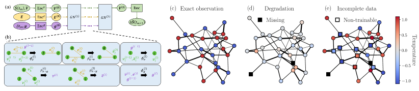
Fig. 1(a) provides a schematic diagram of the NGS at the -th time step. As shown in Eq. (1), the input of the NGS includes and coefficients, which are classified into three types: , and . Additionally, the NGS receives the adjacency matrix of the graph and the time step as inputs. We employ the GNN as the NGS’s fundamental architecture to simulate complex systems characterized by graph domains of varying sizes and topologies. In particular, a graph network (GN) [44] describes a wide range of operations that GNNs can perform. This encompasses updating edge and global features addressing functionalities beyond what a conventional message-passing neural network [45] can accomplish. This flexible GNN structure allows the NGS to effectively model complex dynamics governed by diverse equations.
The input vectors are encoded into higher-dimensional latent vectors , , and through corresponding encoders. These latent vectors then undergo updates through distinct GN layers, utilizing the input adjacency matrix. Each GN layer, shown in Fig. 1(b), consists of three trainable neural netowrks: update functions , and . Additionally, each layer includes three non-trainable, permutation-invariant aggregation functions: , and . Following the sequence of GN layers, is decoded to and the output is computed as .
The NGS is trained to reduce the mean squared error (MSE) between predicted and true states across all nodes and time points, defined as follows:
| (2) |
This training procedure is fully data-driven, which does not require any prior knowledge of the governing equations. Detailed computation of the NGS can be found in the Methods III.2.
To account for the incomplete data, Gaussian noise with a standard deviation of is introduced, and a fraction of nodes are randomly labeled as missing in the training dataset. Figs. 1(c) and (d) illustrate random states of the thermal system and its corresponding degradation. The NGS is trained using the MSE defined in Eq. (2), ensuring a homogeneous fit across all nodes. This approach facilitates robust predictions in the presence of zero-mean noise. Meanwhile, for the NGS of depth , predictions for nodes up to the -th nearest neighbors of missing nodes (marked by squares in Fig. 1(e)) are inaccurate. Excluding these nodes from the MSE allows the NGS to effectively train on incomplete data with missing values. To streamline the experiments, we employ and . Results for additional values of and can be found in the supplementary information (SI).
Once trained, the NGS autoregressively simulates the system using the graph, IC, and coefficients. Starting with , it recursively predicts subsequent values based on its previous output . The use of GNNs allows the NGS to operate independently of the underlying graph’s topology and size. That is, the NGS can be trained on small systems where data acquisition is easy and then applied to simulate larger systems that require more computational resources. Furthermore, as the dynamical system is time-invariant, the NGS simulation can be extended beyond the training periods.
I.3 Extrapolation and Generalization
In this study, we consider two sets of graphs differing in size: and . The NGS is trained on graphs sampled from evaluated for graph extrapolation on , which is at least 20 times larger than the former. Detailed descriptions of the graph domains can be found in the Methods III.3. Regarding time domains, we consider two intervals: and . The model is trained on and evaluated for the time extrapolation on .
Considering the profound impact of ICs and coefficients on dynamical systems, it is standard practice to simulate under different ICs and coefficients. To demonstrate the NGS’s robustness across diverse conditions, we choose a range of ICs and coefficients that allow the systems to exhibit various trajectories. To obtain accurate trajectories, simulations are performed using DOP853 numerical solver [42], which utilizes the 8th-order Runge-Kutta method and adaptive time step techniques.
I.4 Linear systems
A thermal system defined in the graph has a governing equation, which is as follows:
| (3) |
Each node in the system has a temperature , with edges between nodes characterized by a dissipation rate . The temperature change of a node linearly depends on and the temperature difference from its neighbors. This allows the thermal system to exhibit a relatively simple trajectory and is one of the few complex systems for which an analytical solution is known. In our study, we set , which precedes thermodynamic equilibrium where all node temperatures become constant. For detailed implementation specifics, please refer to the Methods III.4.
I.4.1 Reconstruction of Incomplete Data
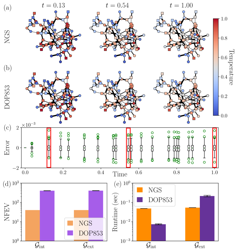
We first assess the reconstruction accuracy of the NGS from incomplete data. Figs. 2 (a) and (b) show the evolution of a thermal system simulated by the trained NGS and DOP853, respectively. Nodes that were labeled as missing during training are marked with squares. As shown, the NGS accurately simulates the temperature evolution across the system, effectively handling missing values and varying temperature change rates.
The discrepancies between the trajectories simulated by the NGS and DOP853 are shown in Fig. 2(c). The error magnitude across all nodes is approximately or less. To quantify the precision, we define the mean absolute error (MAE), including the missing nodes, as follows:
| (4) |
We measured for the reconstruction of the incomplete data with a 95% confidence interval (CI). Note that the MAE of the Gaussian noise of is which is two times larger than the reconstruction MAE.
I.4.2 Robust Simulation
Next, we examine the interpolation and extrapolation across both graph and time domains. The first row of Table. 1 lists the MAEs in the thermal system, accompanied by 95% CIs. The NGS model used for these evaluations is identical to the one trained in the previous section, without additional fine-tuning.
In interpolation, new samples are drawn from and , featuring different initial conditions and coefficients from those used during training. This task assesses the NGS’s ability to generalize across varying initial conditions and coefficients, crucial for robust simulation. The consistent MAEs between reconstruction and interpolation within the error bars demonstrate the NGS’s effectiveness in both tasks.
Regarding graph extrapolation, minimal discrepancies in MAE between and fall within the error bars. Time domain extrapolation involves predicting trajectories beyond the training period, extending simulations into across both graph domains. The MAEs at are marginally larger than those at , though they remain small relative to the temperature magnitude. This behavior is common in iterative numerical solvers, where predictions are made autoregressively, leading to an accumulation of errors over time.
| MAE | |||
| Thermal | |||
| Coupled | |||
| Rössler | |||
I.4.3 Efficient Simulation
The NGS achieves precise simulation while imposing less computational demands than numerical solvers. To quantify the computational workload, we employ a metric known as the number of function evaluations (NFEV). This metric counts the evaluations of the governing equation or neural network required to compute the entire trajectory. For numerical solvers using adaptive time steps, the NFEV is dictated by the solver itself. In contrast, the NGS requires a fixed number of evaluations , because it takes as input and directly predicts the next state. In the meantime, the governing equation evaluation involves complicated CPU operations, whereas the NGS operations primarily entail matrix multiplications optimized for parallel computation on the GPU. Therefore, runtime measurements alongside NFEV are crucial for comparing real-world computational speed.
Figs. 2 (d) and (e) show the NFEV and runtime of both NGS and DOP853, for simulation on and , with time domain of . The NGS demonstrates approximately a 10-fold reduction in the NFEV compared to the DOP853 solver, regardless of the graph size. Note that a direct comparison of the runtime is inappropriate, as the two solvers are executed on different hardware. However, as the system size grows to , the NGS exhibits superior scalability.
I.5 Chaotic systems
Thereafter, we apply the NGS to a coupled Rössler system governed by Eq. (5), composed of Rössler attractors constrained by pairwise attractive interactions.
| (5) |
Each node represents Rössler attractor in a three-dimensional Euclidean space, characterized by coordinates , coupled along the -axis with coupling constants . Large values of can result in a synchronized state, where the positions of a subset or all attractors evolve together [46, 47]. Therefore, we choose small values of to ensure non-trivial trajectories. Global coefficients , , and are selected to induce chaotic behavior in the system. Under these conditions, each attractor exhibits oscillatory motion in the XY plane and occasional excursions in the Z axis at specific times. Given the extended time required for attractors to deviate from the XY plane, we set . For detailed configuration and simulation of the coupled Rössler system, refer to the Methods III.5.
I.5.1 Reliability and Efficiency
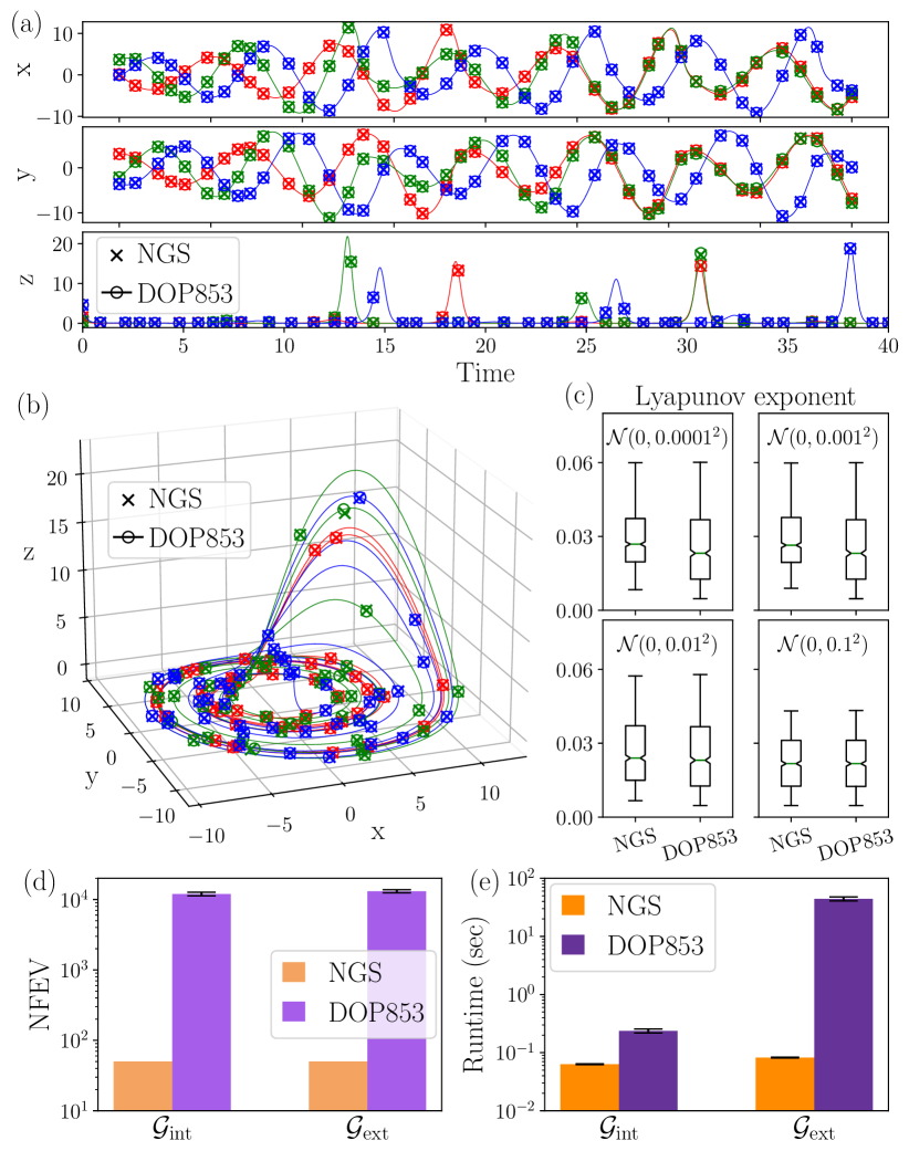
The evolution of the coupled Rössler system is shown in Figs. 3(a) and (b). Three nodes from the system are highlighted with distinct colors. Each node behaves like a typical Rössler attractor, occasionally synchronizing due to pairwise interactions, notably observed between the red and green nodes in . Predictions by the NGS at non-uniform time points, indicated by crosses, closely match the corresponding circles representing DOP853 simulations. The MAE of the reconstruction samples is measured at .
By choosing coefficients , , and to ensure that the coupled Rössler system exhibits chaotic behavior, the discrepancy between trajectories with an IC difference grows exponentially with a Lyapunov exponent as . Fig. 3(c) shows the for both the NGS and DOP853 simulations, considering drawn from a normal distribution with different standard deviations. Although the NGS does not eradicate the inherent of the system, it is comparable to that of a numerical solver.
The second row of Table. 1 summarizes the interpolation and extrapolation MAE in the chaotic system. Similar to the linear system, the reconstruction and interpolation MAE are consistent within the error bars, with minimal differences between and . However, owing to the chaotic nature of the system, discrepancies between and are more pronounced than in the linear system.
The two efficiency metrics, NFEV and runtime, are illustrated in Figs. 3 (d) and (e), respectively. The differences in NFEV and runtime are more apparent than in the linear case, considering the complexity of the trajectory. In both graph domains and , the NGS shows a significant efficiency improvement, requiring over 100 times fewer function evaluations compared to DOP853. The runtime of DOP853 increases by 100 times on , whereas the increase in runtime for the NGS is negligible.
I.6 Stiff problems
Next, the NGS is extended to stiff problems.
| (6) |
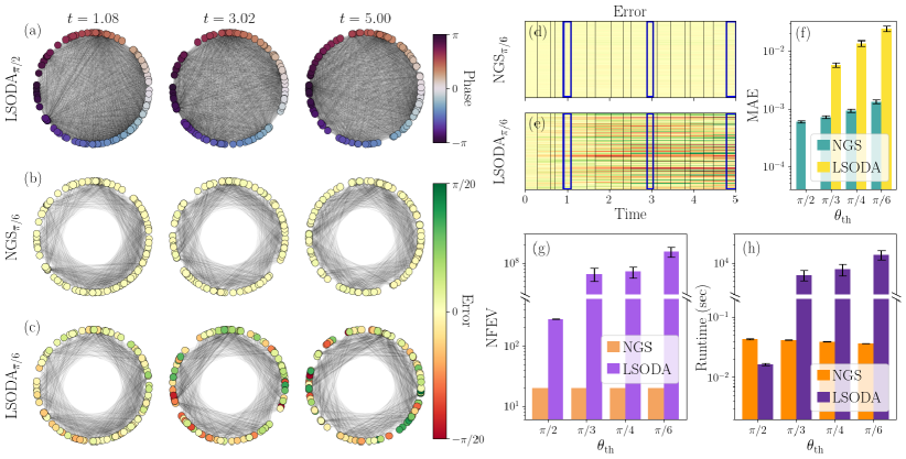
We consider the Kuramoto system, which describes the dynamics of interacting oscillators with nonlinear couplings. Each oscillator has a phase , which evolves according to natural angular velocity and couplings with the other oscillators. As with the coupled Rössler system, we consider a small to avoid synchronization, whereby a subset or all oscillators are in the same phase. This allows the NGS to predict rich trajectories. is set to predict the evolution. Further details regarding the selection of coefficients and the system are outlined in the Methods III.6.
To accurately simulate the system, it is imperative to consider all the interactions; however, the computation of all interactions becomes unmanageable as the system grows. With a little prior knowledge of the target system, it may be feasible to circumvent this problem. For instance, interactions between nodes are stronger when the phase difference is near either or . Accordingly, one may compute interaction between and only when satisfies or . Here, is a threshold that determines the extent of interactions to be ignored. When , all interactions are considered.
Computing a subset of the interactions can be implemented for the numerical solvers and the NGS. However, because the graph structure changes with each evaluation, this problem becomes stiff as the state of each node undergoes erratic changes. Therefore, we employ the LSODA [43], which incorporates automated stiffness detection and uses an implicit method when encountering stiffness, as a substitute for an explicit solver, DOP853. Figs. 4(g) and (h) illustrate the stiffness of this problem, indicating that even for the LSODA, requires a significantly greater NFEV and runtime than case.
Figs. 4(a)-(c) illustrate the snapshots of Kuramoto system, employing LSODA with , NGS with , and LSODA with , respectively. The position of each node is the phase simulated by the corresponding solvers. In the exact simulation of Fig. 4(a), the colors again represent their phases, while in Figs. 4(b) and (c), the errors are illustrated. While the errors of the NGS are considerably small to be visible, those of the LSODA are discernible. The accumulation of error is evident in Figs. 4(d) and (e), where the error for all non-uniform evaluation times is depicted.
Fig. 4(f) shows the MAE of both NGS and LSODA, using different . In , the MAE of LSODA is zero as all interactions are considered; however, for , the errors drastically increase due to the increased number of ignored interactions. In comparison, the increase in MAE for the NGS is a negligible deviation.
In addition to an accurate simulation, the NGS demonstrates greater computational efficiency than numerical solvers. Figs. 4 (g) and (h) show the NFEV and runtime of both NGS and LSODA with four different . As the simulations become stiff problems, the numerical solver requires approximately NFEV, which demands a significantly long runtime. Conversely, the NGS has a -independent NFEV of , and its runtime decreases as the number of edges is reduced as is decreased.
I.7 Traffic forecasting
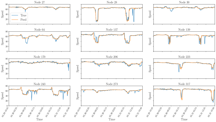
Finally, the NGS is employed in a real-world multivariate time series prediction task, specifically traffic forecasting. We employ a well-known large-scale traffic dataset: PEMS-BAY [30]. In the dataset, the traffic speeds at specific points along the road are recorded at 5-minute intervals. These record points are the nodes in the graph, and the road networks are provided as follows:
| (7) |
where is a directed distance between node and , is the standard deviation of the distances, and is the threshold. The PEMS-BAY dataset comprises 325 nodes and 52,116 time steps.
We employ various baseline models with different properties which can be categorized as follows:
-
•
Models that do not utilize spatial information, relying solely on temporal information: HA (Historical Average), ARIMA with Kalman filter, SVR (Support Vector Regression), and FC-LSTM [48].
- •
- •
- •
- •
The comparison of NGS with the baselines is summarized in Table. 2. The accuracy of predictions is measured using three widely used metrics in traffic forecasting benchmark datasets: MAE, Root Mean Squared Error (RMSE), and Mean Absolute Percentage Error (MAPE). Detailed explanations of baseline models and metrics are provided in Methods section III.7. The visualization of the NGS prediction for several nodes are presented in the SI.
| Dataset | Models | 15 min (3 steps) | 30 min (6 steps) | 60 min (12 steps) | ||||||||
| MAE | RMSE | MAPE | MAE | RMSE | MAPE | MAE | RMSE | MAPE | ||||
| PEMS-BAY | HA | 2.88 | 5.59 | 6.80 | 2.88 | 5.59 | 6.80 | 2.88 | 5.59 | 6.80 | ||
| SVR | 1.85 | 3.49 | 3.80 | 2.48 | 5.18 | 5.50 | 3.28 | 7.08 | 8.00 | |||
| ARIMA | 1.62 | 3.30 | 3.50 | 2.33 | 4.76 | 5.40 | 3.38 | 6.50 | 8.30 | |||
| FC-LSTM | 2.05 | 4.19 | 4.80 | 2.20 | 4.55 | 5.20 | 2.37 | 4.96 | 5.70 | |||
| DCRNN | 1.38 | 2.95 | 2.90 | 1.74 | 3.97 | 3.90 | 2.07 | 4.74 | 4.90 | |||
| Graph WaveNet | 1.30 | 2.74 | 2.73 | 1.63 | 3.70 | 3.67 | 1.95 | 4.52 | 4.63 | |||
| GMAN | 1.34 | 2.91 | 2.86 | 1.63 | 3.76 | 3.68 | 1.86 | 4.32 | 4.37 | |||
| RGDAN | 1.31 | 2.79 | 2.77 | 1.56 | 3.55 | 3.47 | 1.82 | 4.20 | 4.28 | |||
| AGCRN | 1.37 | 2.87 | 2.94 | 1.69 | 3.85 | 3.87 | 1.96 | 4.54 | 4.64 | |||
| MTGNN | 1.32 | 2.79 | 2.77 | 1.65 | 3.74 | 3.69 | 1.94 | 4.49 | 4.53 | |||
| DGCRN | 1.28 | 2.69 | 2.66 | 1.59 | 3.63 | 3.55 | 1.89 | 4.42 | 4.43 | |||
| STEP∗ | 1.26 | 2.73 | 2.59 | 1.55 | 3.58 | 3.43 | 1.79 | 4.20 | 4.18 | |||
| STD-MAE∗ | 1.23 | 2.62 | 2.56 | 1.53 | 3.53 | 3.42 | 1.77 | 4.20 | 4.17 | |||
| NGS | 1.29 | 2.79 | 2.71 | 1.60 | 3.70 | 3.61 | 1.86 | 4.35 | 4.36 | |||
Note that the NGS used to obtain Table. 2 is composed of only MLP elements, as was the case in previous experiments. Nevertheless, its performance is comparable to that of the other state-of-the-art models that employ sophisticated neural network structures, such as LSTM or attention mechanisms and that are specifically designed for traffic forecasting.
II Discussion
In this study, we propose a Neural Graph Simulator (NGS) designed to simulate time-invariant autonomous dynamical systems defined on graphs. By employing a GNN with broad expressive power, the NGS computes the evolution of various dynamical systems within a unified neural network framework. This architecture, optimized for complex systems, can be applied to graphs with different topologies and sizes. It utilizes a non-uniform time step and autoregressive approach, imposing no constraints on evaluation time points.
The NGS’s unique features translate into several significant advantages over traditional numerical solvers. Notably, it does not require prior knowledge of the governing equations, which is a major benefit. In exchange for the absence of equations, training data, which may be noisy or missing, is required. To address this, we implemented a robust training scheme that allows for accurate trajectory reconstruction. Furthermore, the NGS is adaptable to different (ICs) and coefficients, and its computational efficiency surpasses that of advanced numerical solvers. Unlike these solvers, which require numerous evaluations with small time steps, the NGS operates efficiently with only the externally requested number of time steps, demonstrating scalability and efficacy with respect to system size.
The superiority of the NGS is initially demonstrated in a linear system. When applied to a chaotic system, the NGS maintains accuracy while reducing computational costs by over 100 times compared to traditional methods. Its performance is further highlighted in stiff problems, where it improves over times compared to numerical solvers and offers accuracy enhanced by a factor of 10.
Finally, the NGS is applied to the traffic forecasting task to ascertain its applicability to real-world problems. Despite its simple structure, the NGS predicts a traffic flow as accurately as state-of-the-art models employing sophisticated structures.
The versatility of the NGS extends beyond the cases presented in this study, offering various potential avenues for enhancement. For instance, in complex systems with unknown graphs, the NGS can be combined with various techniques to infer adjacency matrices [57]. Additionally, Euclidean space can be adaptively discretized into tessellation lattices, which can be viewed as a specific type of graph. Given its applicability to temporal graphs, such as those in the Kuramoto system, and its flexibility in handling varying time steps, the NGS is expected to achieve more accurate and faster simulations than conventional solvers.
III Methods
III.1 Numerical Simulation
We employ two numerical solvers for the simulation: DOP853 and LSODA. The DOP853 solver is a family of explicit Runge-Kutta solvers equipped with an adaptive step size mechanism. It computes the next state using the 8th-order Runge-Kutta method, while a 5th-order approximation is conducted to estimate the local error at each step. If the local error exceeds a certain tolerance, the solver reduces the step size.
The LSODA employs the Adams method as its primary solver, which is an explicit linear multistep solver that implements an adaptive step size scheme. When the estimated local error exceeds the specified tolerance, LSODA identifies the stiffness and switches to the implicit backward differentiation formula.
The tolerance for local errors exerts a significant influence on the precision of the solution, with the value provided as , where is the solution’s value. To obtain a precise trajectory in the level of double-precision, we choose .
Both the DOP853 and LSODA solvers are adopted from the implementations in the Scipy package. To achieve comparable execution times in C language, we employ a Just-In-Time (JIT) compilation for the numerical solvers, implemented by the Numba package. In contrast, no acceleration techniques, such as JIT compilation, are not utilized when measuring the performance of the NGS. Therefore, it can be expected that further performance gains can be achieved. All simulations are conducted on an Intel i9-10920X CPU, and experiments on NGS are performed on an Nvidia RTX 2080ti GPU.
III.2 NGS Architecture
Inputs. The inputs of the NGS include the current state , constant coefficients , the adjacency matrix of the graph, and time step . As described in Sec. I.1, can be categorized into three types: node, edge, and global features. and are concatenated to node and global features, respectively, and the adjacency matrix is used in the GN layers.
Encoder. As illustrated in Fig. 1(a), three types of input features are encoded into a high-dimensional latent vector by corresponding encoders, which are the neural networks of arbitrary architecture. To leverage the parameter-sharing property of the GNNs, we share the node encoder across all the node features . Similarly, all the edge features are embedded by sharing the edge encoder . As only a single exists per graph, the graph encoder is not shared.
Graph Networks. As shown in Fig. 1(b), the computation of the -th GN layer commences with updating edge features. The edge features are updated in parallel by sharing the per-edge update function , whose inputs are the embedded features of the edge itself, two connecting nodes, and the global.
| (8) |
The updated edge feature is aggregated into the corresponding node feature by a permutation-invariant operation such as sum or mean.
| (9) |
As with the update of the edge feature, the node feature is updated in parallel by sharing the per-node update function , whose inputs are the features of the node itself, aggregated edge, and global.
| (10) |
These updated node and edge features are aggregated using permutation-invariant operations over the entire graph.
| (11) |
Finally, the global feature is updated using the global update function , which takes the aggregated node and edge features and global features from the previous layer as input.
| (12) |
Decoder. Following the sequence of GN layers, a decoder is used to output . Similar to the encoding process, a single neural network is shared across all latent node features . Finally, the next state is computed as .
To demonstrate the performance of the NGS in the simplest architectural configuration, a two-layer multi-layer perceptron (MLP) with GeLU activation is implemented for all encoders () and the decoder (Dec). For the GN layers, we choose , and the architectures of three update functions are two-layer MLP with GeLU activation to maintain the same spirit with the encoders and decoder.
In the majority of physical systems, the state change of a node is affected by the union of its interactions with all of its neighbors. This observation results in the choice of summation operation for . Meanwhile, for the NGS to be effective for different sizes of and , the summation operation is unsuitable for both and . Instead, we select the minimum operation, which is a simple permutation-invariant operation. Formally, we write the three aggregation functions as follows:
| (13) |
Note that the architectural changes to the neural networks or employing different aggregation functions may result in enhanced performance or improved efficiency, depending on the dynamical system.
To train the NGS, we employ the AdamW optimizer with a weight decay factor of to prevent overfitting of the training dataset. Additionally, cosine annealing learning rate scheduling [58] is implemented to identify optimal parameters with lower loss while accelerating a faster convergence rate. Finally, the exponentially weighted moving average is introduced into the parameter space of the neural network [59], thereby facilitating a stable learning process and improving generalization performance.
III.3 Experiment Settings
Here, we consider two sets of Erdős-Rényi random graphs [60] with different sizes: and . The first set, denoted by , comprises graphs with a number of nodes and a number of edges . The second set consists of graphs with and , which are more than 20 times larger than those in . This choice of graph domains allows for efficient training of the NGS and evaluation of its extrapolation ability to graph domains.
Considering the graph domain, we define two-time domains: and . Since the dynamical systems possess disparate time scales of change, each system requires a different time domain to ensure sufficient evolution. The specific values employed in each system are presented together when the system is introduced.
To train the NGS model, 1000 samples are randomly drawn from and . Of these, 800 are allocated for training, while the remaining samples are used for validation. Appropriate ICs and constant coefficients are randomly assigned to determine one trajectory for each graph and time domain. For the interpolation and extrapolation tasks, 50 new systems are sampled from the corresponding graph and time domains.
III.4 Thermal system
The temperature of each node is given as the initial condition of the thermal system. They are randomly assigned to one of two states: hot () or cold (), while the ratio between these two states is randomly determined within .
The coefficients in the system comprise dissipation rates , which are randomly selected from . Together with the time domain of and , the system exhibits various state evolutions, before reaching thermal equilibrium. The time steps between non-uniform evaluation times are randomly sampled from a uniform distribution with .
The heat equation is one of the few governing equations defined on a graph for which an analytical solution is known.
| (14) |
Using the Laplacian matrix of the graph, weighted by dissipation rate as defined in Eq. (14), the spectral solution of the heat equation can be obtained. From the th eigenvalue of and the corresponding normalized eigenvector , the temperature at time of the th node is given as
| (15) |
Here, is the initial condition dependent value defined as .
Due to its reliance on the eigenvalue decomposition of a Laplacian matrix, computing the analytical solution requires order of complexity. Since it is practically infeasible for with thousands of nodes, we employ the DOP853 solver over the analytical solution.
III.5 Coupled Rössler system
The coupled Rössler system, where all nodes are Rössler attractors, evolves according to Eq. (5). The initial condition of the system defines the position of each attractor in three-dimensional space. The and coordinates of each node are randomly set within , while the coordinate is randomly selected from , ensuring diverse trajectories.
The trajectory changes drastically depending on the coefficients , and , potentially altering its characteristics. To impose the most challenging simulation, we select coefficients and , where the attractors exhibit chaotic behaviors. Despite each attractor’s chaotic evolution, synchronization, where all or some of the attractors converge and move together, is avoided to prevent trivial trajectories. To achieve this, we randomly selected from the small range , in which synchronization does not occur.
A Rössler attractor oscillates in the XY plane and exhibits sudden jumps in the Z axis at specific times. These jumps occur after an extended period, necessitating a long training interval . Accordingly, we set , with time steps .
When measuring the Lyapunov exponent , we use the average Euclidean distance between nodes as the discrepancy .
| (16) |
III.6 Fully connected Kuramoto system
In the fully connected Kuramoto system governed by Eq. 6, the initial condition is expressed as a set of uniformly distributed random phases within the interval .
Assuming the distribution of , denoted by , has a mean of zero and satisfies the symmetric condition , the Kuramoto system exhibits a continuous synchronization transition with a critical point . For our study, we employ , resulting in . is randomly chosen from the range to prevent partial or global synchronization.
If the interaction between oscillators is ignored, the nodes rotate with an average period of . To ensure that the NGS predicts the trajectories of nodes that have undergone multiple rotations or have never rotated, we restrict the evaluation to a short-time domain . The time steps are randomly selected from .
Given that the state of the node is the phase , we provide as input to the NGS, accommodating its periodic nature.
III.7 Traffic forecasting
In accordance with the previous research, the PEMS-BAY dataset is divided into training, validation, and test sets in a 7:1:2 ratio and the speed values are subjected to Z-score normalization. The 12-step historical data is provided as the input of the NGS, while the output is the prediction of the subsequent 12 steps. In addition, both in Eq. (7) and the time stamp, represented by time in day and day in week are provided as input. For the state, the time stamps are normalized into the range of , and the corresponding values of cosine and sine are provided along with the normalized speed. The edge coefficient is determined by due to the inverse relationship between the distance and speed correlation. Given that the time steps between all data points are uniform, is a constant value of one. For the global coefficient, the time stamp from the single most recent time point in the historical times is used.
Here, we provide a concise overview of the baseline models utilized in Table. 2.
-
•
HA (Historical Average): This method assumes the traffic flow to be a periodic process and employs a weighted average of historical data to predict future values.
-
•
SVR (Support Vector Regression): A regression technique that uses a support vector machine in a high-dimensional space to predict future speeds.
-
•
ARIMA (Auto-Regressive Integrated Moving Average): A classical time series forecasting model that combines autoregression and moving averages, using differencing to address non-stationarity and capturing trends and seasonality.
-
•
FC-LSTM (Fully Connected LSTM): This model employs a combination of fully connected layers and LSTM modules to construct an encoder-decoder structure that is effective regardless of the structure of time series data.
-
•
DCRNN (Diffusion Convolutional RNN): Capturing both spatial and temporal dependencies by modeling traffic flow as a diffusion process on a directed graph and using a GRU, respectively.
-
•
Graph WaveNet: The model incorporates a self-adaptive adjacency matrix to capture hidden spatial dependencies, and uses stacked dilated 1D convolutions to process long-range temporal sequences.
-
•
GMAN (Graph Multi-Attention Network): Encoder-decoder architecture with multiple spatial-temporal attention blocks, augmented with a gated fusion and transform attention layer to address complex spatial-temporal correlations.
-
•
RGDAN (Random Graph Diffusion Attention Network): In order to extract spatial-temporal correlation, the model combines a graph diffusion attention module and a temporal attention module.
-
•
AGCRN (Adaptive Graph Convolutional Recurrent Network): The model integrates two adaptive modules, one for node-specific patterns and the other for spatial dependencies, which are combined with a GRU.
-
•
MTGNN (Multivariate Time series GNN): The model employs solely the graph structure derived from the graph learning layer, and implements graph and temporal convolutions to capture spatial-temporal properties.
-
•
DGCRN (Dynamic Graph Convolutional Recurrent Network): The hyper-network approach is introduced to generate a dynamic graph, and graph convolution is performed to capture spatial properties. The convolution unit then builds the GRU block, which is used for temporal predictions.
-
•
STEP (Spatial-Temporal GNN Enhanced by Pre-training): The transformer is utilized to discern long-term temporal patterns and to generate segment-level representations in a scalable pre-training model, thereby enhancing the performance of downstream spatial-temporal GNNs.
-
•
STD-MAE (Spatial-Temporal-Decoupled Masked Pre-training): A self-supervised pre-training framework, which employs two decoupled masked autoencoders for the spatial and temporal dimensions. This approach is designed to capture clear and complete spatial-temporal heterogeneity.
The metrics listed in Table. 2 is defined as follows:
| (17) |
where is number of time steps and and represents the predicted and true speed of node at time , respectively.
Acknowledgements.
This work was supported by the National Research Foundation of Korea, South Korea (NRF) Grant No. RS-2023-00279802, KENTECH Research Grant No. KRG2021-01-007 (B.K.), the Creative-Pioneering Researchers Program through Seoul National University, and the NRF Grant No. 2022R1A2C1006871 (J.J.).The fully reproducible codes are available at https://github.com/hoyunchoi/NGS.
References
- Echenique et al. [2004] P. Echenique, J. Gómez-Gardeñes, and Y. Moreno, Improved routing strategies for internet traffic delivery, Phys. Rev. E 70, 056105 (2004).
- Boccaletti et al. [2014] S. Boccaletti, G. Bianconi, R. Criado, C. I. Del Genio, J. Gómez-Gardenes, M. Romance, I. Sendina-Nadal, Z. Wang, and M. Zanin, The structure and dynamics of multilayer networks, Phys. Rep. 544, 1 (2014).
- Schmietendorf et al. [2014] K. Schmietendorf, J. Peinke, R. Friedrich, and O. Kamps, Self-organized synchronization and voltage stability in networks of synchronous machines, Eur. Phys. J. Spec. Top. 223, 2577 (2014).
- Nishikawa and Motter [2015] T. Nishikawa and A. E. Motter, Comparative analysis of existing models for power-grid synchronization, New J. Phys. 17, 015012 (2015).
- Witthaut et al. [2022] D. Witthaut, F. Hellmann, J. Kurths, S. Kettemann, H. Meyer-Ortmanns, and M. Timme, Collective nonlinear dynamics and self-organization in decentralized power grids, Rev. Mod. Phys. 94, 015005 (2022).
- Liu et al. [2003] Z. Liu, Y.-C. Lai, and N. Ye, Propagation and immunization of infection on general networks with both homogeneous and heterogeneous components, Phys. Rev. E 67, 031911 (2003).
- Goltsev et al. [2012] A. V. Goltsev, S. N. Dorogovtsev, J. G. Oliveira, and J. F. Mendes, Localization and spreading of diseases in complex networks, Phys. Rev. Lett. 109, 128702 (2012).
- He et al. [2020] S. He, Y. Peng, and K. Sun, Seir modeling of the covid-19 and its dynamics, Nonlinear Dyn. 101, 1667 (2020).
- Choi et al. [2022] K. Choi, H. Choi, and B. Kahng, Covid-19 epidemic under the k-quarantine model: Network approach, Chaos Solit. 157, 111904 (2022).
- Ernst Hairer [1996] G. W. Ernst Hairer, Solving Ordinary Differential Equations II, 2nd ed., Springer Series in Computational Mathematics, Vol. 14 (Springer Berlin, Heidelberg, 1996).
- Burden and Faires [2016] R. L. Burden and J. D. Faires, Numerical Analysis, 10th ed. (Cengage Learning, 2016).
- Lagaris et al. [1998] I. E. Lagaris, A. Likas, and D. I. Fotiadis, Artificial neural networks for solving ordinary and partial differential equations, IEEE Trans. Neural Netw. 9, 987 (1998).
- Raissi et al. [2019] M. Raissi, P. Perdikaris, and G. E. Karniadakis, Physics-informed neural networks: A deep learning framework for solving forward and inverse problems involving nonlinear partial differential equations, J. Comput. Phys. 378, 686 (2019).
- Karniadakis et al. [2021] G. E. Karniadakis, I. G. Kevrekidis, L. Lu, P. Perdikaris, S. Wang, and L. Yang, Physics-informed machine learning, Nat. Rev. Phys. 3, 422 (2021).
- Cuomo et al. [2022] S. Cuomo, V. S. Di Cola, F. Giampaolo, G. Rozza, M. Raissi, and F. Piccialli, Scientific machine learning through physics–informed neural networks: Where we are and what’s next, J. Sci. Comput. 92, 88 (2022).
- Runge [1895] C. Runge, Über die numerische auflösung von differentialgleichungen, Math. Ann. 46, 167 (1895).
- Kutta [1901] W. Kutta, Beitrag zur näherungsweisen integration totaler differentialgleichungen, Z. Math. Phys. , 435 (1901).
- Gajamannage et al. [2023] K. Gajamannage, D. Jayathilake, Y. Park, and E. Bollt, Recurrent neural networks for dynamical systems: Applications to ordinary differential equations, collective motion, and hydrological modeling, Chaos 33, 013109 (2023).
- Chen et al. [2018] R. T. Q. Chen, Y. Rubanova, J. Bettencourt, and D. K. Duvenaud, Neural ordinary differential equations, in NeurIPS, Vol. 31 (Curran Associates, Inc., 2018).
- Pathak et al. [2018] J. Pathak, B. Hunt, M. Girvan, Z. Lu, and E. Ott, Model-free prediction of large spatiotemporally chaotic systems from data: A reservoir computing approach, Phys. Rev. Lett. 120, 024102 (2018).
- Gauthier et al. [2021] D. J. Gauthier, E. Bollt, A. Griffith, and W. A. Barbosa, Next generation reservoir computing, Nat. Commun. 12, 1 (2021).
- Barbosa and Gauthier [2022] W. A. Barbosa and D. J. Gauthier, Learning spatiotemporal chaos using next-generation reservoir computing, Chaos 32, 093137 (2022).
- Nazerian et al. [2023] A. Nazerian, C. Nathe, J. D. Hart, and F. Sorrentino, Synchronizing chaos using reservoir computing, Chaos 33, 103121 (2023).
- Song et al. [2023] J. U. Song, K. Choi, S. M. Oh, and B. Kahng, Exploring nonlinear dynamics and network structures in kuramoto systems using machine learning approaches, Chaos 33, 073148 (2023).
- Kong et al. [2023] L.-W. Kong, Y. Weng, B. Glaz, M. Haile, and Y.-C. Lai, Reservoir computing as digital twins for nonlinear dynamical systems, Chaos 33, 033111 (2023).
- Gori et al. [2005] M. Gori, G. Monfardini, and F. Scarselli, A new model for learning in graph domains, in Proc. of IJCNN, Vol. 2 (IEEE, 2005) pp. 729–734.
- Scarselli et al. [2009] F. Scarselli, M. Gori, A. C. Tsoi, M. Hagenbuchner, and G. Monfardini, The graph neural network model, IEEE Trans. Neural Netw. 20, 61 (2009).
- Nauck et al. [2022] C. Nauck, M. Lindner, K. Schürholt, H. Zhang, P. Schultz, J. Kurths, I. Isenhardt, and F. Hellmann, Predicting basin stability of power grids using graph neural networks, New J. Phys. 24, 043041 (2022).
- Jhun et al. [2023] B. Jhun, H. Choi, Y. Lee, J. Lee, C. H. Kim, and B. Kahng, Prediction and mitigation of nonlocal cascading failures using graph neural networks, Chaos 33, 013115 (2023).
- Li et al. [2018] Y. Li, R. Yu, C. Shahabi, and Y. Liu, Diffusion convolutional recurrent neural network: Data-driven traffic forecasting, in ICLR, Vol. 6 (ICLR, 2018).
- Sanchez-Gonzalez et al. [2020] A. Sanchez-Gonzalez, J. Godwin, T. Pfaff, R. Ying, J. Leskovec, and P. Battaglia, Learning to simulate complex physics with graph networks, in ICML, Vol. 37 (PMLR, 2020).
- Lu et al. [2021] L. Lu, P. Jin, G. Pang, Z. Zhang, and G. E. Karniadakis, Learning nonlinear operators via deeponet based on the universal approximation theorem of operators, Nat. Mach. Intell. 3, 218 (2021).
- Li et al. [2021] Z. Li, N. B. Kovachki, K. Azizzadenesheli, B. liu, K. Bhattacharya, A. Stuart, and A. Anandkumar, Fourier neural operator for parametric partial differential equations, in ICLR, Vol. 9 (ICLR, 2021).
- Anandkumar et al. [2019] A. Anandkumar, K. Azizzadenesheli, K. Bhattacharya, N. Kovachki, Z. Li, B. Liu, and A. Stuart, Neural operator: Graph kernel network for partial differential equations, in ICLR workshop, Vol. 7 (ICLR, 2019).
- Rudy et al. [2019] S. H. Rudy, J. N. Kutz, and S. L. Brunton, Deep learning of dynamics and signal-noise decomposition with time-stepping constraints, J. Comput. Phys. 396, 483 (2019).
- Lin et al. [2023] Z.-F. Lin, Y.-M. Liang, J.-L. Zhao, J.-R. Li, and T. Kapitaniak, Prediction of dynamic systems driven by lévy noise based on deep learning, Nonlinear Dyn. 111, 1511 (2023).
- Wikner et al. [2024] A. Wikner, J. Harvey, M. Girvan, B. R. Hunt, A. Pomerance, T. Antonsen, and E. Ott, Stabilizing machine learning prediction of dynamics: Novel noise-inspired regularization tested with reservoir computing, Neural Netw. 170, 94 (2024).
- Marisca et al. [2022] I. Marisca, A. Cini, and C. Alippi, Learning to reconstruct missing data from spatiotemporal graphs with sparse observations, in NeurIPS, Vol. 35 (Curran Associates, Inc., 2022).
- Nguyen et al. [2020] D. Nguyen, S. Ouala, L. Drumetz, and R. Fablet, Assimilation-based learning of chaotic dynamical systems from noisy and partial data, in ICASSP, Vol. 45 (IEEE, 2020).
- Huang et al. [2020] Z. Huang, Y. Sun, and W. Wang, Learning continuous system dynamics from irregularly-sampled partial observations, in NeurIPS, Vol. 33 (Curran Associates, Inc., 2020).
- Dormand and Prince [1980] J. R. Dormand and P. J. Prince, A family of embedded runge-kutta formulae, J. Comput. Appl. Math. 6, 19 (1980).
- Hairer et al. [1993] E. Hairer, S. Nørsett, and G. Wanner, Solving Ordinary Differential Equations I, 2nd ed., Springer Series in Computational Mathematics, Vol. 8 (Springer Berlin, Heidelberg, 1993).
- Petzold [1983] L. Petzold, Automatic selection of methods for solving stiff and nonstiff systems of ordinary differential equations, SIAM J. Sci. Comput. 4, 136 (1983).
- Battaglia et al. [2018] P. W. Battaglia, J. B. Hamrick, V. Bapst, A. Sanchez-Gonzalez, V. Zambaldi, M. Malinowski, A. Tacchetti, D. Raposo, A. Santoro, R. Faulkner, C. Gulcehre, F. Song, A. Ballard, J. Gilmer, G. Dahl, A. Vaswani, K. Allen, C. Nash, V. Langston, C. Dyer, N. Heess, D. Wierstra, P. Kohli, M. Botvinick, O. Vinyals, Y. Li, and R. Pascanu, Relational inductive biases, deep learning, and graph networks (2018), arXiv:1806.01261 [cs.LG] .
- Gilmer et al. [2017] J. Gilmer, S. S. Schoenholz, P. F. Riley, O. Vinyals, and G. E. Dahl, Neural message passing for quantum chemistry, in ICML, Vol. 34 (PMLR, 2017).
- Omelchenko et al. [2012] I. Omelchenko, B. Riemenschneider, P. Hövel, Y. Maistrenko, and E. Schöll, Transition from spatial coherence to incoherence in coupled chaotic systems, Phys. Rev. E 85, 026212 (2012).
- Mishra et al. [2015] A. Mishra, C. Hens, M. Bose, P. K. Roy, and S. K. Dana, Chimeralike states in a network of oscillators under attractive and repulsive global coupling, Phys. Rev. E 92, 062920 (2015).
- Sutskever et al. [2014] I. Sutskever, O. Vinyals, and Q. V. Le, Sequence to sequence learning with neural networks, in NeurIPS, Vol. 27 (Curran Associates, Inc., 2014).
- Wu et al. [2019] Z. Wu, S. Pan, G. Long, J. Jiang, and C. Zhang, Graph wavenet for deep spatial-temporal graph modeling, in IJCAI, Vol. 19 (International Joint Conferences on Artificial Intelligence Organization, 2019).
- Zheng et al. [2020] C. Zheng, X. Fan, C. Wang, and J. Qi, Gman: A graph multi-attention network for traffic prediction, in AAAI, Vol. 34 (AAAI Press, 2020).
- Fan et al. [2024] J. Fan, W. Weng, H. Tian, H. Wu, F. Zhu, and J. Wu, Rgdan: A random graph diffusion attention network for traffic prediction, Neural Netw. 172, 106093 (2024).
- Bai et al. [2020] L. Bai, L. Yao, C. Li, X. Wang, and C. Wang, Adaptive graph convolutional recurrent network for traffic forecasting, in NeurIPS, Vol. 33 (Curran Associates, Inc., 2020).
- Wu et al. [2020] Z. Wu, S. Pan, G. Long, J. Jiang, X. Chang, and C. Zhang, Connecting the dots: Multivariate time series forecasting with graph neural networks, in SIGKDD (Association for Computing Machinery, 2020) pp. 753–763.
- Li et al. [2023] F. Li, J. Feng, H. Yan, G. Jin, F. Yang, F. Sun, D. Jin, and Y. Li, Dynamic graph convolutional recurrent network for traffic prediction: Benchmark and solution, ACM Trans. Knowl. Discov. Data 17, 1 (2023).
- Shao et al. [2022] Z. Shao, Z. Zhang, F. Wang, and Y. Xu, Pre-training enhanced spatial-temporal graph neural network for multivariate time series forecasting, in SIGKDD (Association for Computing Machinery, 2022).
- Gao et al. [2024] H. Gao, R. Jiang, Z. Dong, J. Deng, Y. Ma, and X. Song, Spatial-temporal-decoupled masked pre-training for spatiotemporal forecasting, in IJCAI, Vol. 24 (International Joint Conferences on Artificial Intelligence Organization, 2024).
- Pereira et al. [2023] T. Pereira, E. R. dos Santos, and S. van Strien, Robust reconstruction of sparse network dynamics (2023), arXiv:2308.06433 [physics.data-an] .
- Loshchilov and Hutter [2017] I. Loshchilov and F. Hutter, SGDR: Stochastic gradient descent with warm restarts, in ICLR, Vol. 5 (ICLR, 2017).
- Izmailov et al. [2018] P. Izmailov, D. Podoprikhin, T. Garipov, D. Vetrov, and A. G. Wilson, Averaging weights leads to wider optima and better generalization, in UAI, Vol. 34 (AUAI, 2018) pp. 876–885.
- Erdős and Rényi [1960] P. Erdős and A. Rényi, On the evolution of random graphs, Publ. Math. Inst. Hung. Acad. Sci 5, 17 (1960).
S1 Various noise levels and missing ratios
This section presents the performance of NGS as the noise level and the missing fraction of the training data are varied.
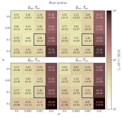
Fig. S1 depicts the mean absolute error (MAE) of the NGS in the thermal system, detailed in Table. I of the main text. The NGS demonstrates robust accuracy across a broad range of and , provided that the training data are free from noise and missing values (). However, accuracy declines as increases to 0.01, where the MAE reaches . The MAE of the NGS is superior to the noise level provided but remains on a comparable scale.
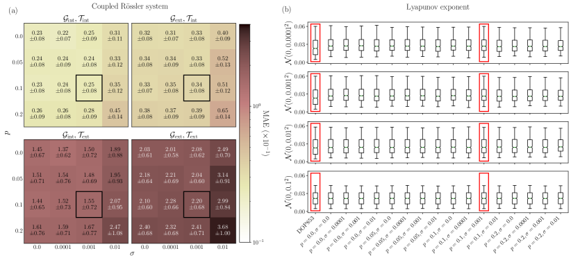
Similar to Fig. S1, the MAE of the NGS trained on the coupled Rössler system with varying and are depicted in Fig. S2(a). As described in Table. I of the main text, the MAE for NGS interpolation () and graph domain extrapolation () are highly commendable. However, the time domain extrapolation () and () exhibit relatively high MAE due to the inherent chaoticity of the system. To address this, the Lyapunov exponents of the NGS trained on various incomplete datasets are presented in Fig. S2(b), analogous to those shown in Fig. 3(c) in the main text. The case of , demonstrated in the main text, is denoted by black and red boxes, respectively.
S2 PEMS-BAY traffic forecasting
Here, we present the result of the NGS prediction on a test dataset from PEMS-BAY for a few randomly selected nodes. The complete set of predictions for the entire network can be accessed via the GitHub repository, referenced in the main text.