FxTS-Net: Fixed-Time Stable Learning Framework for Neural ODEs
Abstract
Neural Ordinary Differential Equations (Neural ODEs), as a novel category of modeling big data methods, cleverly link traditional neural networks and dynamical systems. However, it is challenging to ensure the dynamics system reaches a correctly predicted state within a user-defined fixed time. To address this problem, we propose a new method for training Neural ODEs using fixed-time stability (FxTS) Lyapunov conditions. Our framework, called FxTS-Net, is based on the novel FxTS loss (FxTS-Loss) designed on Lyapunov functions, which aims to encourage convergence to accurate predictions in a user-defined fixed time. We also provide an innovative approach for constructing Lyapunov functions to meet various tasks and network architecture requirements, achieved by leveraging supervised information during training. By developing a more precise time upper bound estimation for bounded non-vanishingly perturbed systems, we demonstrate that minimizing FxTS-Loss not only guarantees FxTS behavior of the dynamics but also input perturbation robustness. For optimising FxTS-Loss, we also propose a learning algorithm, in which the simulated perturbation sampling method can capture sample points in critical regions to approximate FxTS-Loss. Experimentally, we find that FxTS-Net provides better prediction performance and better robustness under input perturbation.
keywords:
Neural ODEs , Fixed-time stability , Adversarial robustness[1]organization=Department of Mathematics, addressline=Sichuan University, city=Chengdu, postcode=Sichuan, 610064, country=China \affiliation[2]organization=Department of Artificial Intelligence and Computer Science, addressline=Yibin University, city=Yibin, postcode=Sichuan, 644000, country=China
1 Introduction
Neural ODEs have emerged as a promising area of research, offering significant advancements in modeling complex, large-scale datasets through continuous dynamical systems. Originating from the reinterpretation of residual networks (ResNets) as continuous-time dynamical systems [1, 2], Neural ODEs extend to model continuous dynamics and address the limitations of discrete architectures [3]. By incorporating techniques from dynamical systems theory, Neural ODEs enable continuous modeling of data and show broad applicability across various domains, including irregular time series modeling [4, 5], generative modeling [6, 7], wind speed prediction [8], and traffic flow forecasting [9].
However, Neural ODEs still face some limitations, particularly in ensuring the stability of the learned system. The standard learning approach, which relies on differentiating through the ODE solution using techniques like the adjoint method [10, 3], struggles to guarantee stable behavior (informally, the tendency of the system to remain within some invariant bounded set). This instability leads to slow convergence and inaccurate predictions [11]. Even more concerning, a dynamical system lacking stability guarantees can result in significant output distortions when subjected to small input perturbations.
Recently, some research has focused on enhancing the stability of Neural ODEs by applying Lyapunov stability theory [11, 12]. Kolter et al. [12] proposed a joint learning approach that integrates Neural ODEs with learnable Lyapunov functions to ensure system stability. However, this approach intensifies the trade-off between stability and accuracy [11]. To alleviate the trade-off, Rodriguez et al. introduced a method for training Neural ODEs using Lyapunov exponential stabilization conditions [11]. Since this method relies on the fact that the output function and loss function must satisfy Lyapunov functions conditions, it hampers the applicability in many real-world application scenarios. Constructing appropriate Lyapunov functions remains a longstanding challenge in dynamical systems and control. Therefore, it is essential to investigate and enrich the techniques for constructing Lyapunov functions further to satisfy the requirements of complex network structures and diverse tasks in practical applications.
Despite recent progress in enhancing Neural ODEs stability, most of the existing methods [11, 12, 13, 14] focus on exponential convergence, neglecting the critical aspect in fixed-time stability. Fixed-time stability is essential in many real-world applications where a system must reliably reach a desired state within a user-defined evolution time. For instance, Cui et al. employed the extensive experimental analysis method to illustrate the critical role of ensuring that a suitable state is reached within a pre-determined time [15]; and further Chu et al. extended the evolutionary time to ensure that the dynamical system reaches the desired state under input perturbations, and improved robustness against adversarial samples [16]. However, to the best of authors’ knowledge, Neural ODEs stability within a pre-determined time has not been considered in the literature. The present paper is thus devoted to the fixed-time stability in Neural ODEs under some mild conditons.
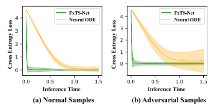
To illustrate the research motivation behind FxTS-Net, we compare FxTS-Net and Neural ODEs in Figure 1. From the orange lines and regions, it indicates that the dynamics of the Neural ODE across the state space do not guarantee stable convergence to correct predictions within a user-defined fixed time. Moreover, input perturbations exacerbate this instability leading to worse convergence speed and prediction accuracy.
In this work, we investigate how to use Lyapunov stability theory to learn fixed-time stable dynamical systems for ensuring the efficientibility and the robustness. Our main contributions can be summerized as follows:
-
1.
To ensure that the learned Neural ODE achieves correct prediction at a user-defined fixed time, we propose FxTS-Net, which enforces fixed-time stable dynamic inference by introducing FxTS-Loss.
-
2.
For various tasks and network structures, we propose a method to construct Lyapunov functions, i.e., embedding sub-optimisation problems in training to exploit supervised information for constructing it.
-
3.
For optimising the FxTS-Loss, we propose a learning algorithm, including the simulated perturbation sampling method, i.e., simulating the input perturbation by perturbing extracted features to generate the post-perturbation integral trajectory, which captures the sampling points of the critical region to approximate the FxTS-Loss.
-
4.
Theoretically, we show that minimizing the FxTS-Loss will 1) guarantee that the dynamical system satisfies the FxTS Lyapunov condition; 2) enable robustness of input perturbations by developing a more precise time upper bound estimation for bounded non-decreasing perturbed dynamics.
-
5.
Experimentally, FxTS-Net is competitive or superior in prediction accuracy and improves robustness against various perturbations. Moreover the experimental results aligns with the theoretical insights, emphasizing the beneficial impact of fixed-time stability on the overall performance of FxTS-Net .
2 Background and Related Work
2.1 Supervised Learning of Neural ODEs
Neural ODEs. Following previous research work [11], we will consider a class of data-controlled Neural ODEs. Let denote the input data pair where belongs to , the mathematical model is
| (1) | |||
| (2) | |||
| (3) |
where is an output function with parameter , likewise is an input function, and let . The idea of the Neural ODE is to use a neural network to parameterize a differential equation that governs the hidden states with respect to time t.
In practice, we set that Equation (2) evolves over the time interval , i.e., the upper limit of the integral , although theoretically it is possible to choose any time to predict . Additionally, we assume that the state space is both bounded and path-connected.
Model Assumption. We impose a Lipschitz continuity assumption on neural networks used in Neural ODEs as follows.
Assumption 2.1.
For any neural network with parameter , there exists a positive constant such that, for all and ,
| (4) |
This assumption is not overly onerous since neural networks with activation functions such as tanh, ReLU, and sigmoid functions generally satisfy the Lipschitz continuity condition in Assumption 2.1 [4, 17, 18].
Supervised Learning. Consider the standard supervised learning setup, where the training set of input-output pairs is denoted as as , the optimization model is
| (5) |
where is shorthand for Equations (1)-(3). The learning goal is to find a parameterization of our model by minimizing a supervised loss over the training data.
Like typical methods in deep learning, the standard approach to training Neural ODEs is backpropagation via Equation (5). Moreover, the end-to-end training optimization problem can be viewed as the following optimal control problem (for brevity, only using a single ), is given by
| (6) | ||||
| s.t. | ||||
It is possible to optimize Equation (6), which can be rolled out of the dynamics using solver backpropagation or concomitant methods [10, 3]. However, in Equation (6), there is no explicit penalty or regularization to ensure the dynamical system reaches a steady state in a user-defined fixed time. Indeed, we can observe such a problem from Figure 1, where the dynamics of Neural ODEs are not guaranteed to stabilize in a fixed time, leading the Neural ODE to learn a fragile solution. In this work, we propose the FxTS-Net approach to address these limitations through a fixed-time control theory learning objective.
2.2 Lyapunov Conditions for Fixed-Time Stability
Intuitively, a fixed-time stable dynamical system means that all solutions in a region around an equilibrium point flow to that point at a prescribed fixed time. The area of Lyapunov theory [19] establishes the connection between the various stability and descent according to a particular type of function known as a Lyapunov function. In this work, we assume that the equilibrium point is .
Definition 2.1 (Lyapunov Function).
A continuously differentiable function is a Lyapunov function if is positive definite function, i.e., for and .
We now recall the fixed-time stability with respect to . The fixed-time stability (FxTS), defined as the following, allows the settling time to remain uniformly bounded for all initial conditions.
Definition 2.2 (FxTS).
For the study of fixed-time stability, it is necessary to introduce the sufficient condition for FxTS of the equilibrium point , which are used to guarantee the convergence of the system trajectory to the equilibrium point in a user-defined fixed time [20], as stated in the following theorem.
Lemma 2.1 (FxTS Condition[20]).
The introduction of FxTS in Neural ODEs is desirable because: 1) it guarantees fast convergence to desired states (as defined by ) after integrating for a fixed time (e.g., for ); 2) it has implications for adversarial robustness. Specifically, we require the learned Neural ODE to satisfy the additional structure specified by Equations (8) and (9) for ensuring the fixed-time stability of the Neural ODE. In Section 3, we will develop a learning framework to find a desired parameter satisfying Equation (9).
2.3 Learning Stable Dynamics
In recent years, many researchers have conducted in-depth studies on how to impose stability on Neural ODEs with various formulations. Using regularization of the flow on perturbed data based on time-invariance and steady-state conditions, Yan et al. proposed TisODE, which outperforms ordinary Neural ODEs in terms of robustness [21]. By introducing contraction theory, Zakwan et al. improved the robustness of Neural ODEs to Gaussian and impulse noise on the MNIST dataset [22]. In addition, Kang et al. imposed Lyapunov stability guarantees around the equilibrium point to eliminate the effects of perturbations in the input [13].
We observe that the above works are devoted to the study of the exponential stability for learning dynamical systems. Generally, setting the final evolution time as a pre-defined fixed one is a common requirement in practice and so it is crucial to ensure the stationarity of the dynamical system solution within a user-defined fixed time. In this work, we propose a fixed-time stabilization learning framework that allows the learned dynamical system to be stabilized within a pre-defined fixed time.
3 Fixed-Time Stable Learning Framework
The intuition behind the proposed approach is straightforward: as mentioned in Section 2.2, our goal is to find the parameters of the Neural ODEs that satisfy the FxTS Lyapunov stability condition (Lemma 2.1). We formulate this approach in two steps:
-
1.
In Section 3.1, for any given output and loss functions, we construct an appropriate Lyapunov function based on the supervised information.
-
2.
In Section 3.2, we design a new FxTS-Loss via the Lyapunov function , which quantifies the degree of violation for the FxTS contraction condition in Equation (9). By optimizing FxTS-Loss, the Neural ODE has a stable evolutionary behavior within a pre-defined fixed time.
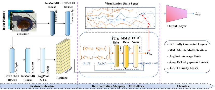
Theoretically, by optimizing FxTS-Loss, we show that the learned Neural ODE stabilizes to the optimal state point such that the supervised loss is minimized at a pre-defined fixed time (Theorem 3.1), and obtain a new adversarial robustness guarantee (Theorem 3.2). The approach architecture can be seen in Figure 2, and the corresponding learning algorithm is described in Section 3.3.
3.1 Constructing Lyapunov Functions Using Supervised Information
Constructing Lyapunov functions has long been a significant challenge in dynamical systems and control, especially for applications involving complex and real-world tasks. This section addresses the challenge by leveraging supervised information to construct Lyapunov functions for applying to real-world tasks regardless of the network architecture or learning objective.
A critical step in constructing a Lyapunov function is identifying the appropriate optimal state . After determining , the Lyapunov function is defined as
| (10) |
which can be used to guarantee convergence of the dynamics to . Recalling the training optimization problem for Neural ODEs, the optimal state needs to satisfy that the supervised loss is zero. For a classification task as an example, with supervised loss and a given input-output pair , the optimal state can be obtained by solving a minimization problem as
| (11) |
where is the output layer as defined in Equation (3). In general, the continuous differentiability of the output layer is easy satisfied, which ensures the feasibility of this approach.
Next we apply a multi-step gradient projection method for solving the optimization problem (11), in which the choice of the initial point is crucial due to the fact that the unsuitable initial point may converge to a worthless for the dynamical system. By choosing a suitable initial point, we can increase the match between and the dynamical system. Specifically, as shown in Figure 2, we first use the solution trajectory in Equations (1)-(3) to determine the initial point , and then locate by the multi-step gradient projection method.
3.2 Fixed-Time Stabilizing Lyapunov Loss
In this subsection, we introduce a fixed-time stabilizing loss function for Neural ODEs, derived from the Lyapunov function defined in Section 3. The goal is to impose fixed-time stability on the learning dynamics by utilizing the stability condition in Equation (9), leading to the formulation of FxTS-Loss. To begin, we define the pointwise version of this loss.
Definition 3.1 (Point-wise FxTS-Loss).
For a single input-output pair and the Lyapunov function defined in Equation (10), a point-wise FxTS-Loss defines as
| (12) |
where , , and with .
This point-wise definition quantifies the degree of violation of the FxTS contraction condition at each local state , which can be interpreted as a local contraction property. To utilize Lemma 2.1, we need to check that is zero for all and such that the dynamics converge to the loss-minimizing prediction within a user-defined fixed time.
Next, we define FxTS-Loss over the coupled distribution (rather than the entire and ) by integrating the pointwise loss over time.
Definition 3.2 (FxTS-Loss).
With the help of Definition 3.2, we end this subsection by giving our first main result. Theorem 3.1, shown below, demonstrates that minimizing FxTS-Loss guarantees fixed-time stability in the learned Neural ODE, with the proof given in A.1.
Theorem 3.1.
Under the setting of Definition 3.2, if there exists a parameter of the dynamical system that attains , then for almost everywhere :
-
1.
For any , the inference dynamical system satisfies .
- 2.
3.3 Robust learning Algorithms
It is crucial to choose the appropriate set and ensure that is equal to zero throughout . Although Theorem 3.1 shows that the dynamical system convergences to the state in a fixed time by minimizing the FxTS-Loss which formulates on the set of trajectories , it should be noticed that this stability depends on the integration trajectory, leading to a lack of robustness against input perturbations. Specifically, the choice of in Theorem 3.1 is so tight that a small input perturbation may change the integral trajectory of the dynamical system beyond the range of .
Therefore, such a challenge in designing robust learning algorithms lies in computing the inner integral in Equation (13), which requires addressing two key problems:
-
1.
Selecting an appropriate that enables the learned Neural ODEs to exhibit robustness.
-
2.
Collecting sample points to approximate the FxTS-Loss over with limited computational resources.
To tackle these key problems, we propose a simulated perturbation sampling method. As illustrated in the state space visualization in Figure 2, we simulate input perturbations by perturbation extracting perturbation features to generate the post-perturbation integral trajectory (as shown by the orange curve in the figure) and subsequently sample this trajectory. The pseudo-code for the robust learning algorithm is provided in Algorithm 2.1. This method effectively collects sampling points in the critical regions of the Neural ODE, thereby enhancing both robustness and accuracy.
3.4 Adversarial Robustness
It is well known that small perturbations at the input of an unstable dynamical system will lead to large distortions in the system’s output. This section will explore the provable adversarial robustness obtained by minimizing the FxTS-Loss, which utilizes robust control based on Lyapunov stability theory. Robust control fundamentally ensures that a system remains stable when perturbed, and the notion is closely related to the study of adversarial robustness in machine learning [24, 25].
Firstly, to obtain adversarial robustness guarantees, we develop more precise time upper bound estimation for non-vanishingly perturbed systems [19, Section 9.2]. Specifically, considering the dynamical system in Equations (1)-(3), for an input perturbation, we can utilize the Lipschitz continuity from Assumption 2.1 to transform the perturbed dynamics into the original dynamics with a bounded nonvanishing perturbation.
Moreover, we relax FxTS Lyapunov conditions in Equation (9) by allowing a constant term to appear in the upper bound of the time derivative of the Lyapunov function. The FxTS Lyapunov condition is considered for a positive definite, proper, continuously differentiable as follows
| (15) |
where , , , and . Remark that if , then Lyapunov condition (15) is reduced to Equation (9). Proposition 3.1, shown below, provides the expression for the time upper bound estimation of the equation (15), with the proof given in A.2.
Proposition 3.1.
Let , and such that . Let and with . Define
| (16) |
Then, for all , the following conclusions hold:
-
1.
For , one has
-
2.
For , one obtains
where , .
-
3.
For , it holds that
where , .
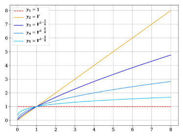
It is worth mentioning that Proposition 3.1 provides more precise estimations for both the upper bound on time and the boundary than the ones in [23]. In fact, Garg [23] scaled Equation (15) by multiplying on to solve the failure in integration due to the introduction of a constant term. This means that the convergence boundary also needs to satisfy , besides multiplying is not the best choice for scaling. In Proposition 3.1, we multiply for more accurate estimation and by introducing to eliminate the condition . In Figure 3, we visualize the different scaling techniques and can see that our scaling technique is having a tighter effect. Notably, when is selected as , our estimation results are precise and error-free.
| Dataset | Method | Orignal | Gaussian | Shot | Impulse | Speckle | Motion | Avg |
|---|---|---|---|---|---|---|---|---|
| Fashion-MNIST | ResNet18 | 8.44 | 16.37 | 14.47 | 41.15 | 9.18 | 12.35 | 16.99 |
| Neural ODE | 8.33 | 15.96 | 14.90 | 40.69 | 9.50 | 12.18 | 16.93 | |
| LyaNet | 8.12 | 15.09 | 13.22 | 40.43 | 9.08 | 12.83 | 16.46 | |
| FxTS-Net | 8.08 | 14.68 | 14.10 | 32.60 | 9.15 | 11.74 | 15.06 | |
| CIFAR10 | ResNet18 | 18.35 | 51.38 | 55.93 | 60.60 | 24.88 | 26.87 | 39.67 |
| Neural ODE | 17.64 | 48.42 | 53.04 | 57.32 | 23.94 | 24.92 | 37.55 | |
| LyaNet | 17.53 | 46.78 | 50.40 | 54.84 | 23.35 | 24.65 | 36.26 | |
| FxTS-Net | 16.21 | 43.96 | 48.90 | 52.64 | 21.63 | 24.47 | 34.64 | |
| CIFAR100 | ResNet18 | 41.43 | 71.84 | 73.98 | 79.75 | 45.75 | 46.96 | 59.95 |
| Neural ODE | 41.27 | 70.94 | 73.03 | 79.22 | 45.61 | 46.27 | 59.39 | |
| LyaNet | 40.48 | 69.41 | 71.90 | 77.25 | 45.68 | 46.30 | 58.50 | |
| FxTS-Net | 39.07 | 67.92 | 69.84 | 76.47 | 43.25 | 44.42 | 56.83 |
Secondly, we use Proposition 3.1 to further show that optimizing FxTS-Loss can obtain robustness guarantees. Let denote the input-output pair, and be the solution of the dynamical system defined in Equations (1)-(3). Consider to be a perturbed version of the input data such that
| (17) |
where represents the degree of perturbation. Suppose that we consider the supervised learning task mentioned in Section 2 and use to represent the perturbed version of .
Theorem 3.2.
See A.3 for the proof. Basically, Theorem 3.2 provides the stabilization to a neighborhood of origin (the radius of the neighborhood is proportional to the perturbation magnitude) at a fixed time for the difference between the perturbed outputs and label . It is worth saying that the radius of the neighborhood can be effectively reduced by setting the appropriate and in the learning. In contrast, the lack of such stability in other Neural ODEs can yield dramatically different solutions from small changes in the input data, causing dramatic performance degradation.
4 Experiments
In this section, we conduct a series of comprehensive experiments to evaluate the performance of our proposed FxTS-Net model. Our analysis aims to address the following key research questions:
-
1.
RQ1: How does FxTS-Net perform in terms of classification accuracy compared to baseline models?
-
2.
RQ2: How robust is FxTS-Net against various types of perturbations, including stochastic noise and adversarial attacks?
-
3.
RQ3: What impact does the fixed-time stability guarantee have on the decision boundaries of FxTS-Net compared to traditional Neural ODEs?
-
4.
RQ4: How do different parameters affect the performance of FxTS-Net?
Through these experiments, we provide a comprehensive analysis of the model’s performance and robustness across various settings, highlighting the advantages of incorporating fixed-time stability.
4.1 Experimental settings
This subsection provides a detailed overview of the experimental setup, including the datasets used, training configurations, and evaluation metrics employed to assess the performance and robustness of FxTS-Net.
| Dataset | Method | FGSM | BIM | PGD | APGD | ||||
|---|---|---|---|---|---|---|---|---|---|
| 8/255 | 16/255 | 8/255 | 16/255 | 8/255 | 16/255 | 8/255 | 16/255 | ||
| Fashion-MNIST | ResNet18 | 52.46 | 62.84 | 23.84 | 27.46 | 36.52 | 37.44 | 39.56 | 39.81 |
| Neural ODE | 42.40 | 51.20 | 21.85 | 23.93 | 30.75 | 31.67 | 32.91 | 33.01 | |
| LyaNet | 30.76 | 33.77 | 11.97 | 12.54 | 27.87 | 28.45 | 29.74 | 30.27 | |
| FxTS-Net | 25.85 | 26.06 | 8.28 | 8.41 | 24.72 | 27.14 | 26.94 | 27.21 | |
| CIFAR10 | ResNet18 | 49.39 | 60.45 | 35.28 | 39.13 | 37.58 | 38.27 | 40.93 | 42.17 |
| Neural ODE | 49.86 | 59.90 | 37.09 | 40.94 | 38.20 | 39.96 | 42.01 | 44.05 | |
| LyaNet | 44.23 | 51.03 | 27.11 | 28.12 | 38.30 | 39.28 | 41.58 | 42.63 | |
| FxTS-Net | 37.37 | 38.33 | 19.15 | 19.96 | 36.03 | 37.25 | 39.48 | 40.17 | |
| CIFAR100 | ResNet18 | 84.73 | 87.20 | 62.72 | 65.52 | 82.34 | 83.31 | 84.98 | 85.13 |
| Neural ODE | 84.69 | 87.03 | 62.86 | 65.34 | 81.96 | 82.34 | 84.65 | 84.97 | |
| LyaNet | 81.24 | 81.84 | 55.92 | 56.33 | 80.45 | 80.97 | 83.38 | 83.93 | |
| FxTS-Net | 80.00 | 80.72 | 56.77 | 57.54 | 78.82 | 79.72 | 81.49 | 81.58 | |
Datasets. We evaluate our method on three classification datasets: Fashion-MNIST [26], CIFAR-10, and CIFAR-100 [27]. Fashion-MNIST consists of 70,000 grayscale images (28×28 pixels) across 10 classes, with 60,000 used for training and 10,000 for testing. CIFAR-10 and CIFAR-100 contain 60,000 color images (32×32 pixels), with 50,000 images for training and 10,000 for testing, categorized into 10 and 100 classes, respectively.
Training Details. Our implementation is based on the open-source codes.111https://github.com/ivandariojr/LyapunovLearning The Runge-Kutta method [10] is still used as numerical solvers in the process of forward propagation. Following [11] to simplify tuning, we trained models using Nero [28] with a learning rate of 0.01, a batch size 64 for LyaNet and Ours, and 128 for other models. All models were trained for a total of 120 epochs. In our model, we set inner learning rate , inner iterations , samples , and time discretization resolution .
Evaluation Details. Model performance is measured by classification error on the test sets of Fashion-MNIST, CIFAR-10, and CIFAR-100. Following [15, 21], robustness is assessed using two types of perturbations: stochastic noise and adversarial attacks. For stochastic noise, we apply Gaussian, shot, impulse, speckle, and motion noise [29]. For adversarial robustness, we consider the Fast Gradient Sign Method (FGSM) [30], Basic Iterative Method (BIM) [31], Projected Gradient Descent (PGD) [32], and Auto Projected Gradient Descent (APGD) [33].
We compare three models:
-
1.
ResNet-18 [34]: A conventional convolutional neural network where the residual connections approximate Eulerian integrated dynamical systems.
-
2.
Neural ODEs [11]: A data-controlled Neural ODE framework using ResNet-18 as a feature extractor.
-
3.
LyaNet [11]: A stable Neural ODE model that guarantees exponential stability via the Lyapunov exponential stability condition.
4.2 Accuracy and Robustness Against Stochastic Noises
This subsection focuses on the classification errors on standard and noise-perturbed images, with a fixed maximum evolution time of . The results, detailed in Table 1, show that FxTS-Net consistently outperforms the benchmark models across all datasets. Specifically, FxTS-Net achieves a 0.04%, 1.32%, and 1.41% improvement in standard classification accuracy than the best one of other models on Fashion-MNIST, CIFAR-10, and CIFAR-100, respectively. This demonstrates that our fixed-time stable learning framework enables Neural ODEs to make accurate predictions within a pre-defined time, effectively enhancing classification performance.
Moreover, FxTS-Net exhibits improved robustness on noise-perturbed data, achieving the best average performance across all random noise types. Although it lags slightly behind LyaNet by 0.07% in speckle noise and 0.88% in shot noise for Fashion-MNIST, FxTS-Net remains highly competitive. These results emphasize the robustness of FxTS-Net to small input perturbations, validating our model’s ability to regulate the dynamic behavior of Neural ODEs and enhance stability. This aligns with our initial motivation to improve the robustness of Neural ODEs against random noise perturbations.
4.3 Robustness Against Adversarial Attacks
Similar to our evaluation of randomly noisy images, we evaluated the adversarial robustness of FxTS-Net and the benchmark models within a fixed evolutionary time Each model was tested on Fashion-MNIST, CIFAR-10, and CIFAR-100 datasets, using adversarial perturbations with attack radii of and from FGSM, BIM, PGD, and APGD attacks, as detailed in Table 2.
Specifically, on Fashion-MNIST and CIFAR-10, FxTS-Net consistently outperforms the other models across all attacks. For CIFAR-100, FxTS-Net demonstrates superior robustness across FGSM, PGD, and APGD attacks and only slightly lags behind LyaNet by 0.85% and 1.21% in the BIM attack. The observed improvement underscores the efficacy of our robust learning algorithm, which effectively captures key sample points in critical regions to compute the FxTS-Loss. This facilitates the local-global structure alignment of the Lyapunov condition, confirming the importance of stability guarantees within pre-defined fixed times for Neural ODEs. The results also support our theoretical analysis, showing that efficiently approximating FxTS-Loss enhances robustness to adversarial attacks.
| Parameters | Orignal | Gaussian | Impulse | Speckle | Motion | FGSM | BIM | APGD | Avg |
|---|---|---|---|---|---|---|---|---|---|
| 16.06 | 46.44 | 55.39 | 22.80 | 25.16 | 37.90 | 19.65 | 39.78 | 32.90 | |
| 16.15 | 44.82 | 53.27 | 22.03 | 25.45 | 37.67 | 19.58 | 39.92 | 32.36 | |
| 16.21 | 43.96 | 52.64 | 21.63 | 24.47 | 37.37 | 19.15 | 39.48 | 31.86 | |
| 16.74 | 44.28 | 52.74 | 21.88 | 23.81 | 37.53 | 19.42 | 39.75 | 32.01 |
4.4 Inspecting Decision Boundaries
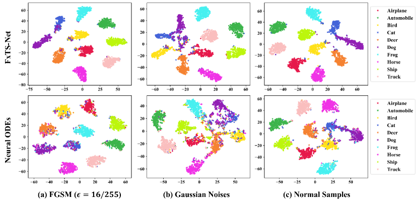
In this subsection, we further investigate the impact of introducing fixed-time stability guarantees on the decision boundaries learned by Neural ODEs. We perform a TSNE clustering analysis on the classification features of Neural ODEs and FxTS-Net using adversarial perturbations from FGSM attacks, Gaussian noise, and clean CIFAR-10 data. The results, shown in Figure 4, highlight clear differences between the models. For standard data, FxTS-Net demonstrates a more distinct separation between clusters of different categories compared to Neural ODEs. Notably, under Gaussian noise, the decision boundaries of Neural ODEs become highly blurred, whereas FxTS-Net maintains sharp boundaries. This illustrates how the fixed-time stability framework enhances the model’s decision boundaries and mitigates boundary ambiguity under noisy conditions.
Moreover, while Gaussian noise causes boundary-blurring, FGSM perturbations do not blur the decision boundaries but directly confuse the classification outcomes. Even under adversarial attacks, FxTS-Net consistently delivers better classification performance than Neural ODEs, which strongly supports the effectiveness of our approach. In summary, FxTS-Net excels in maintaining stable decision boundaries and classification accuracy across various data perturbations, validating the role of fixed-time stability in improving both the robustness and classification performance of Neural ODEs.
4.5 Ablation Study of Parameters
In this subsection, we conduct ablation experiments to explore the effects of different parameters in FxTS-Net, using CIFAR10 as the dataset. Firstly, we conduct an ablation study of the algorithm’s maximum perturbation radius . Secondly, we conduct experiments for the parameters in the FxTS-Loss function to assess their impact on the robustness under various conditions. Additional ablation study results are described in Appendix B. These experiments aim to reveal the key role of each parameter on the stability and noise robustness of FxTS-Net, to guide parameter selection.
The first part of the experiment investigates the effect of the perturbation radius . The results in Table 3 demonstrate that smaller values of (e.g., 0.4) can lead to better performance on clean data but at the expense of robustness under adversarial conditions. Conversely, increasing to 1.2 achieves the best overall performance across both original and adversarial data, with the highest average accuracy. This indicates that moderate perturbations during training encourage the model to generalize well across different types of inputs, thereby enhancing its robustness. However, for larger values of , FxTS-Net exhibits diminishing returns, indicating an optimal disturbance range for balancing accuracy and robustness.
| Parameters | Orignal | Gaussian | Impulse | Speckle | Motion | FGSM | BIM | APGD | Avg |
|---|---|---|---|---|---|---|---|---|---|
| 17.10 | 44.87 | 52.71 | 22.56 | 25.51 | 37.86 | 19.72 | 39.79 | 32.52 | |
| 16.57 | 45.24 | 53.60 | 22.09 | 24.66 | 37.59 | 19.13 | 39.87 | 32.34 | |
| 16.94 | 45.98 | 54.53 | 22.48 | 25.29 | 37.86 | 19.84 | 40.03 | 32.87 | |
| 17.41 | 44.88 | 53.47 | 22.35 | 25.47 | 38.03 | 20.02 | 39.74 | 32.67 | |
| 16.21 | 43.96 | 52.64 | 21.63 | 24.47 | 37.37 | 19.15 | 39.48 | 31.86 | |
| 16.70 | 44.11 | 52.78 | 22.18 | 25.11 | 37.56 | 19.86 | 39.59 | 32.24 |
In the second part, we explore how different combinations of , , and affect model performance. As shown in Table 4 , the parameter combination shows the best results on both raw and attack data (including FGSM and motion blur), especially on the average error of 31.86%. It is also shown that the larger value of , compared to , leads to better accuracy and robustness of the model, while the variation of between 2.0 and 3.0 has less impact on the final results.
In summary, the ablation study highlights the importance of tuning both the loss function parameters and disturbance radius to balance between accuracy and robustness. The results demonstrate that the combination of , , and provides the best overall performance, particularly in adversarial settings.
5 Conclusion
In this work, we introduce FxTS-Net, a framework for ensuring fixed-time stability of Neural ODEs by incorporating novel FxTS Lyapunov losses. We develop a more precise time upper bound estimation for bounded non-decreasing perturbation systems, providing a theoretical foundation for extending Neural ODEs to fixed-time stabilization and addressing their theoretical guarantees regarding adversarial robustness.
Furthermore, we present a method for constructing Lyapunov functions by utilizing supervised information during training, which can be adapted to the requirements of different tasks and network structures. We also provide learning algorithms, including capturing sample points in the critical region to approximate the FxTS-Loss, which promotes the local-global structure of the Lyapunov condition. Our experimental results demonstrated the effectiveness of FxTS-Net in improving adversarial robustness while maintaining competitive classification accuracy.
While our approach demonstrates competitive classification accuracy and robustness, several avenues remain for future exploration. One is the extension of FxTS-Net to more complex and high-dimensional tasks, such as video classification or 3D spatial data modeling. The other is the exploration of FxTS-Net to integrate with some known adversarial defense mechanisms, which ensures stronger robustness.
Declaration of competing interest
The authors declare that they have no known competing financial interests or personal relationships that could have appeared to influence the work reported in this paper.
Acknowledgement
This work was supported by the National Natural Science Foundation of China (12171339, 12471296).
References
- Haber and Ruthotto [2017] E. Haber, L. Ruthotto, Stable architectures for deep neural networks, Inverse Problems 34 (1) (2017) 014004.
- Ruthotto and Haber [2020] L. Ruthotto, E. Haber, Deep Neural Networks Motivated by Partial Differential Equations, Journal of Mathematical Imaging and Vision 62 (3) (2020) 352–364.
- Kidger et al. [2021a] P. Kidger, R. T. Q. Chen, T. J. Lyons, “Hey, that’s not an ODE”: Faster ODE Adjoints via Seminorms, in: Proceedings of the 38th International Conference on Machine Learning, vol. 139, 5443–5452, 2021a.
- Oh et al. [2024] Y. Oh, D. Lim, S. Kim, Stable Neural Stochastic Differential Equations in Analyzing Irregular Time Series Data, in: The Twelfth International Conference on Learning Representations, 2024.
- Kidger et al. [2020] P. Kidger, J. Morrill, J. Foster, T. Lyons, Neural Controlled Differential Equations for Irregular Time Series, in: Advances in Neural Information Processing Systems, vol. 33, 6696–6707, 2020.
- Yildiz et al. [2019] C. Yildiz, M. Heinonen, H. Lahdesmaki, ODE2VAE: Deep generative second order ODEs with Bayesian neural networks, in: Advances in Neural Information Processing Systems, vol. 32, 2019.
- Kidger et al. [2021b] P. Kidger, J. Foster, X. Li, T. J. Lyons, Neural SDEs as Infinite-Dimensional GANs, in: Proceedings of the 38th International Conference on Machine Learning, vol. 139, 5453–5463, 2021b.
- Ye et al. [2022] R. Ye, X. Li, Y. Ye, B. Zhang, DynamicNet: A time-variant ODE network for multi-step wind speed prediction, Neural Networks 152 (2022) 118–139.
- Chu et al. [2024a] Z. Chu, W. Ma, M. Li, H. Chen, Adaptive Decision Spatio-temporal neural ODE for traffic flow forecasting with Multi-Kernel Temporal Dynamic Dilation Convolution, Neural Networks 179 (2024a) 106549.
- Chen et al. [2018] R. T. Q. Chen, Y. Rubanova, J. Bettencourt, D. K. Duvenaud, Neural Ordinary Differential Equations, in: Advances in Neural Information Processing Systems, vol. 31, 2018.
- Rodriguez et al. [2022] I. D. J. Rodriguez, A. Ames, Y. Yue, LyaNet: A Lyapunov Framework for Training Neural ODEs, in: Proceedings of the 39th International Conference on Machine Learning, vol. 162, 18687–18703, 2022.
- Kolter and Manek [2019] J. Z. Kolter, G. Manek, Learning Stable Deep Dynamics Models, in: Advances in Neural Information Processing Systems, vol. 32, 2019.
- Kang et al. [2021] Q. Kang, Y. Song, Q. Ding, W. P. Tay, Stable Neural ODE with Lyapunov-Stable Equilibrium Points for Defending Against Adversarial Attacks, in: Advances in Neural Information Processing Systems, vol. 34, 14925–14937, 2021.
- Zhao et al. [2023] K. Zhao, Q. Kang, Y. Song, R. She, S. Wang, W. P. Tay, Adversarial Robustness in Graph Neural Networks: A Hamiltonian Approach, in: Advances in Neural Information Processing Systems, vol. 36, 3338–3361, 2023.
- Cui et al. [2023] W. Cui, H. Zhang, H. Chu, P. Hu, Y. Li, On robustness of neural ODEs image classifiers, Information Sciences 632 (2023) 576–593.
- Chu et al. [2024b] H. Chu, S. Wei, Q. Lu, Y. Zhao, Improving neural ordinary differential equations via knowledge distillation, IET Computer Vision 18 (2) (2024b) 304–314.
- Fazlyab et al. [2019] M. Fazlyab, A. Robey, H. Hassani, M. Morari, G. Pappas, Efficient and Accurate Estimation of Lipschitz Constants for Deep Neural Networks, in: Advances in Neural Information Processing Systems, vol. 32, 2019.
- Latorre et al. [2020] F. Latorre, P. Rolland, V. Cevher, Lipschitz constant estimation of Neural Networks via sparse polynomial optimization, in: International Conference on Learning Representations, 2020.
- Khalil [2002] H. K. Khalil, Nonlinear systems; 3rd ed., Prentice-Hall, Upper Saddle River, NJ, 2002.
- Garg et al. [2022] K. Garg, E. Arabi, D. Panagou, Fixed-time control under spatiotemporal and input constraints: A Quadratic Programming based approach, Automatica 141 (2022) 110314.
- YAN et al. [2020] H. YAN, J. DU, V. TAN, J. FENG, On Robustness of Neural Ordinary Differential Equations, in: International Conference on Learning Representations, 2020.
- Zakwan et al. [2023] M. Zakwan, L. Xu, G. Ferrari-Trecate, Robust Classification Using Contractive Hamiltonian Neural ODEs, IEEE Control Systems Letters 7 (2023) 145–150.
- Garg [2021] K. Garg, Advances in the theory of fixed-time stability with applications in constrained control and optimization, Ph.D. thesis, University of Michigan, Horace H. Rackham School of Graduate Studies, 2021.
- Wang et al. [2024] R. Wang, H. Ke, M. Hu, W. Wu, Adversarially robust neural networks with feature uncertainty learning and label embedding, Neural Networks 172 (2024) 106087.
- Li et al. [2023] J. Li, S. Zhang, J. Cao, M. Tan, Learning defense transformations for counterattacking adversarial examples, Neural Networks 164 (2023) 177–185.
- Xiao [2017] H. Xiao, Fashion-mnist: a novel image dataset for benchmarking machine learning algorithms, arXiv preprint arXiv:1708.07747 .
- Krizhevsky et al. [2009] A. Krizhevsky, et al., Learning multiple layers of features from tiny images .
- Liu et al. [2021] Y. Liu, J. Bernstein, M. Meister, Y. Yue, Learning by Turning: Neural Architecture Aware Optimisation, in: Proceedings of the 38th International Conference on Machine Learning, vol. 139, 6748–6758, 2021.
- Hendrycks and Dietterich [2019] D. Hendrycks, T. Dietterich, Benchmarking Neural Network Robustness to Common Corruptions and Perturbations, in: International Conference on Learning Representations, 2019.
- Goodfellow et al. [2014] I. J. Goodfellow, J. Shlens, C. Szegedy, Explaining and harnessing adversarial examples, arXiv preprint arXiv:1412.6572 .
- Kurakin et al. [2018] A. Kurakin, I. J. Goodfellow, S. Bengio, Adversarial examples in the physical world, Chapman and Hall/CRC, 2018.
- Madry et al. [2018] A. Madry, A. Makelov, L. Schmidt, D. Tsipras, A. Vladu, Towards Deep Learning Models Resistant to Adversarial Attacks, in: International Conference on Learning Representations, 2018.
- Croce and Hein [2020] F. Croce, M. Hein, Reliable evaluation of adversarial robustness with an ensemble of diverse parameter-free attacks, in: Proceedings of the 37th International Conference on Machine Learning, vol. 119, 2206–2216, 2020.
- He et al. [2016] K. He, X. Zhang, S. Ren, J. Sun, Deep Residual Learning for Image Recognition, in: Proceedings of the IEEE Conference on Computer Vision and Pattern Recognition (CVPR), 770–778, 2016.
Appendix A Theoretical Proofs
A.1 Proof of Theorem 3.1
Proof.
We begin by recalling that
| (18) |
Clearly, . We can see that is continuous for any , , , and . In fact, the continuity of can be attributed to its nature as the maximum of two continuous functions. Now we rearrange the integral terms in Equation (13) in the following form
| (19) |
We first claim that, when , equals zero for almost everywhere and any . Assume to the contrary that there exist and non-zero measurement set such that , i.e., there is a constant making . Since is continuous, there exists a -neighborhood such that for any and . Thus, one has
| (20) | ||||
| (21) | ||||
| (22) |
which contradicts the assumption , and so for almost everywhere and any .
Next we show the second result. By the definition of and the first result, we have the following inequality
| (23) |
where , , and with . It follows from Lemma 2.1 that , which is desired. ∎
A.2 Proof of Proposition 3.1
Proof.
Firstly, for , it holds that
| (24) |
due to the fact that for all . Substituting , we have , , and . It follows that
| (25) |
Clearly, for all , which implies that the integral of the last equation in (25) exists. Thus,
| (26) |
Taking and into above equation yields the desired result.
Secondly, for , it holds that
| (27) |
due to the fact that for all . Similarly, for , we have
| (28) |
Since , one has for all . Thus, the integral of the last equation in (28) exists. Find , , and such that
| (29) |
which is equivalent to
| (30) |
Thus, we have
| (31) |
Since , one has
| (32) |
It follows from Equation (28) that
Taking and into above equation yields desired result.
Finally, for , it holds that
| (33) |
due to the fact that for all . Similarly, for , we have
| (34) |
Obviously, the integral of the last equation in (34) exists. It follows that
| (35) |
Taking and into above equation yields desired result. ∎
A.3 Proof of Theorem 3.2
Proof.
We will use the notation for the time derivative of as follows
Thus it follows that
| (36) |
In order to use the Comparison Principle of differential equations, consider an auxiliary differential equation given by
| (37) |
Let such that . Then it follows that with . By using Proposition 3.1, we can conclude that
-
1.
Since , one has . For , we can obtain an estimate of the fixed time as follows
(38) -
2.
Since , one has . By the fact that , for , we can obtain an estimate of the fixed time as follows
(39) -
3.
Since , one has . By the fact that , for , we can obtain an estimate of the fixed time as follows
(40) where .
In summary, when , for any , one has with . Thus, we obtain with , which is desired. ∎
Appendix B Experiments
| Parameters | Orignal | Gaussian | Impulse | Speckle | Motion | FGSM | BIM | APGD | Avg |
|---|---|---|---|---|---|---|---|---|---|
| 17.31 | 45.81 | 55.17 | 22.45 | 25.66 | 37.94 | 19.73 | 40.06 | 33.02 | |
| 16.99 | 44.79 | 53.50 | 22.43 | 25.17 | 37.82 | 19.73 | 40.17 | 32.58 | |
| 16.91 | 44.27 | 53.32 | 22.56 | 24.91 | 37.80 | 19.81 | 39.89 | 32.43 | |
| 16.80 | 44.48 | 53.08 | 21.79 | 24.37 | 37.40 | 19.75 | 39.52 | 32.15 | |
| 16.21 | 43.96 | 52.64 | 21.63 | 24.47 | 37.37 | 19.15 | 39.48 | 31.86 | |
| 16.64 | 43.44 | 52.83 | 22.15 | 25.46 | 37.87 | 19.64 | 39.74 | 32.22 | |
| 17.37 | 45.69 | 54.38 | 22.53 | 25.32 | 37.66 | 19.96 | 39.98 | 32.86 |
Following the settings of Section 4.5, we investigated the impact of the inner learning rate on the classification performance and robustness of FxTS-Net, where the parameter varies between 0.4 and 2.8. Table 5 shows a general decreasing trend in classification error as increases, with the smallest error of 16.21% at on the original data. consistently showed strong performance for adversarial attacks and noise, producing the lowest average classification error (31.86%). While larger values of slightly reduce robustness, increasing too much (e.g., ) tends to increase classification error, especially with Gaussian and impulse noise. The optimal value of is around , which balances accuracy and robustness to various perturbations.
| Parameters | Orignal | Gaussian | Impulse | Speckle | Motion | FGSM | BIM | APGD | AVG |
|---|---|---|---|---|---|---|---|---|---|
| 16.79 | 43.79 | 53.00 | 22.13 | 25.23 | 37.45 | 19.71 | 39.59 | 32.21 | |
| 16.21 | 43.96 | 52.64 | 21.63 | 24.47 | 37.37 | 19.15 | 39.48 | 31.86 | |
| 16.69 | 44.70 | 53.27 | 21.41 | 24.64 | 38.32 | 19.94 | 40.31 | 32.41 | |
| 16.73 | 44.60 | 53.28 | 22.46 | 24.69 | 38.13 | 19.71 | 40.26 | 32.48 | |
| 17.00 | 45.26 | 53.70 | 22.04 | 24.83 | 38.12 | 19.95 | 40.45 | 32.67 | |
| 17.03 | 45.54 | 54.20 | 22.29 | 25.80 | 38.32 | 20.04 | 40.39 | 32.95 |
We consider the effect of the trajectory sampling resolution and the number of perturbation samples on the model performance, where satisfies . As shown in Table 6, the configuration and achieves the lowest classification error on both clean data and robustness. As increases beyond 5, the model’s robustness to perturbations starts to degrade, as shown by the increasing average error, particularly for . Similarly, decreasing the number of perturbation samples leads to poorer performance, likely due to the reduced diversity in the perturbation space that the model is exposed to during training. The combination of and strikes an optimal balance between model robustness and classification accuracy. Higher values of or lower values of lead to a deterioration in performance, indicating that careful tuning of both parameters is critical for robustness