Magnetic response of topological insulator layer with metamaterial substrate induced by an electric point source

Abstract

Topological insulators (TIs) are materials with unique surface conductive properties that distinguish them from normal insulators and have attracted significant interest due to their potential applications in electronics and spintronics. However, their weak magnetic field response in traditional setups has limited practical applications. Here, we show that integrating TIs with active metamaterial substrates can significantly enhance the induced magnetic field by more than $10^{4}$ times. Our results demonstrate that selecting specific permittivity and permeability values for the active metamaterial substrate optimizes the magnetic field at the interface between the TI layer and the metamaterial, extending into free space. This represents a substantial improvement over previous methods, where the magnetic field decayed rapidly. The findings reveal that the TI-metamaterial approach enhances the magnetic field response, unveiling new aspects of TI electromagnetic behavior and suggesting novel pathways for developing materials with tailored electromagnetic properties. The integration of metamaterials with TIs offers promising opportunities for advancements in materials science and various technological applications. Overall, our study provides a practical and effective approach to exploring the unique magnetic field responses of TIs, potentially benefiting other complex material systems.

• July 2024

Keywords: Topological Insulator; Metamaterial; Magnetic Field Enhancement; Hybrid Layer Structure

1 Introduction

The study of topological insulators (TIs), materials with a unique topological order, represents a significant step forward in developing new electronics. These materials are insulators internally but have conductive surfaces [1, 2, 3, 4]. The ability to have conductive edge states without an external magnetic field, as demonstrated in the quantum spin Hall effect in two-dimensional TIs, highlights their potential for transforming electronic devices.

The special properties of TIs have created novel applications that are not possible with conventional insulators. Qi et al. [5] demonstrated that an electric charge near a TI surface induces a magnetic monopole due to the topological magneto-electric effect. Martín-Ruiz et al. [6, 7] used the Green’s function method to study boundary effects and special electromagnetic properties in TIs with Chern-Simons extended electrodynamics. The research by Lai et al. [8] explored the tunability of plasmons in TIs, showing their potential in plasmonics and spintronics. Wang et al. [9] discussed intrinsic magnetic TIs, such as MnBi₂Te₄, which combine magnetism with topological properties, leading to new quantum phenomena.

Meanwhile, synthetic topological insulator structures [10, 11], such as nanowires and nanoribbons, are being explored in field-effect transistors (FETs), optoelectronic devices, memory storage devices and magnetoelectric devices [12, 13, 14, 15, 16]. These structures exhibit enhanced surface conduction due to their high surface-to-volume ratio and can improve the performance of devices like photodetectors, spintronic, and quantum computing systems [17, 18, 19] by leveraging their unique surface properties and quantum effects.

The novel magnetic field response of TIs is an area of growing interest due to its potential applications in advanced technology. The unique topological electromagnetic properties of TIs are key to understanding their novel magnetic field responses, although these effects are usually small. To enhance their electronic and magnetic properties, the development of layered structures incorporating TIs has been proposed [20]. In 2011, Burkov and Balents [21] proposed Weyl semimetal states in TI multilayers to achieve unusual electronic states. Further studies explored TI-ferromagnet multilayers [22] for efficient spin-orbit torque [23, 24], highlighting practical applications in spintronic devices [25]. In 2020, An et al. [26] demonstrated significant polarization rotation in multilayer TI structures, enhancing optical applications. Additionally, Ardakani and Zare (2021) [27] showed strong Faraday rotation using dielectric multilayers with a single TI layer with improved magnetic field interactions.

Most of the work reviewed above focuses on the dynamic effects. In this work, we explore the novel magnetic field response of topological insulators (TIs) when exposed to a static electric point source. This static response, which couples electric and magnetic fields, distinguishes TIs from normal insulators more significantly than their dynamic behavior. However, as demonstrated by Qi et al. [5], the induced magnetic field by a TI is very weak, making it challenging to harness for practical applications. To address this challenge, we explore the magnetic field response of TIs in composite layered structures, particularly with metamaterials.

Metamaterials have been a significant area of research since the late 20th century, with their unique properties offering potential for various technological applications. The concept was first theoretically proposed by Victor Veselago in 1968 [28], who suggested that materials could exhibit both negative permittivity and permeability, resulting in a negative refractive index. This idea, though intriguing, remained largely theoretical until the development of practical metamaterials in the early 2000s [29]. In 2000, Smith and Kroll [30] demonstrated negative refraction in left-handed materials, a groundbreaking experimental validation that paved the way for further research and development. Following this, Shelby et al. [31] provided experimental verification of a negative index of refraction using a metamaterial constructed from an array of copper split-ring resonators and wires. Liu et al. [32] introduced dynamic and tunable metamaterials that can be electrically controlled, using vanadium dioxide to achieve multifunctional control. This marked a significant advancement, enabling the modulation of metamaterial properties through external stimuli, thereby enhancing their practical applicability. Most recently, Castles et al. in 2020 [33] explored active metamaterials with static electric susceptibility less than one. This work demonstrated that active metamaterials could manipulate static electric susceptibility, a property that had been theoretically suggested but never experimentally confirmed until then.

In this work, we focus on the magnetic response of TIs by integrating them with multi-layer composite structures with metamaterials. By employing the unique electromagnetic properties of TIs and metamaterials, we investigate the magnetic response induced by an electric charge. This study explores a novel approach to enhancing the magnetic field response of TIs, highlighting unique electromagnetic interactions within TIs and opening new avenues for their practical application in advanced technologies.

2 Model

For a standard dielectric material, we have $\bi{D}=(\epsilon_{0}\epsilon_{r})\bi{E}$ for electric displacement, $\bi{D}$, and electric field, $\bi{E}$, with $\epsilon_{0}$ and $\epsilon_{r}$ being the vacuum permittivity and relative permittivity of the material, respectively; and $\bi{H}=\bi{B}/(\mu_{0}\mu_{r})$ for magnetic induction strength, $\bi{B}$ and field, $\bi{H}$, with $\mu_{0}$ and $\mu_{r}$ being the vacuum permeability and relative permeability of the material, respectively. These equations illustrate that, typically, the electric and magnetic fields in a dielectric material are independent of each other. However, this independence does not apply to chiral materials, such as TIs, which exhibit a coupling between electric and magnetic fields. Specifically, for TIs, the constitutive equations become:

$$\bi{D} =\epsilon_{0}\epsilon_{r}\bi{E}-\frac{\alpha\theta}{\pi}\epsilon_{0}c\bi{B},$$ (1a)

$$\bi{H} =\frac{\bi{B}}{\mu_{0}\mu_{r}}+\frac{\alpha\theta}{\pi}\frac{1}{\mu_{0}c}\bi{E},$$ (1b)

where $\theta$ is the topological phase of the TI, $c$ is the speed of light and $\alpha$ is the fine structure constant.

In scenarios where the TI has a substantial thickness (beyond a few dozens of nanometers), the TI phase, $\theta$, stabilises as a constant throughout the material, as illustrated in Fig. 1. As such, we have $\nabla\theta=\mathbf{0}$ within the TI, while phase transitions are confined to thin layers (less than a few nanometers) at the interfaces between the TI and its surrounding environment, which indicates that these transitions can be accounted for by adjusting boundary conditions. Considering the setup displayed in Fig. 1, without any free charges the macroscopic Maxwell’s equations are $\nabla\cdot\bi{D}=0$ and $\nabla\cdot\bi{B}=0$. As such, from Eq. (1), we obtain

$$\bi{\nabla}\bi{\cdot}\bi{E} =0,\qquad\bi{\nabla}\bi{\cdot}\bi{B} =0.$$ (1b)

Given these conditions, for static problems, the electric and magnetic fields can be expressed in terms of electric ($\phi_{E}$) and magnetic ($\phi_{B}$) potentials as

$$\bi{E}=-\nabla\phi_{E},\qquad\bi{B}=-\nabla\phi_{B}.$$ (1c)

Both potentials satisfy the Laplace equation, as

$$\nabla^{2}\phi=0$$ (1d)

with $\phi$ representing either $\phi_{E}$ or $\phi_{B}$.

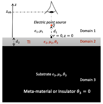
Figure 1: Sketch of induced magnetic monopole of TI from an electric point charge by multi-layer composite composed with TI, normal insulators, $\mu$-metals.

In the context of a two-layer structure as depicted in Fig. 1, where domain 2 is a TI layer with thickness of $d_{2}$, and domain 3 represents an infinitely thick structure, we consider the free space above the TI layer as domain 1 with relative permittivity $\epsilon_{1}=1$ and relative permeability $\mu_{1}=1$. A static electric point charge $Q$ is located $d_{1}$ above the top surface of the TI layer (domain 2). Our model generalises the two layers as TIs, each characterised by specific material properties: $\epsilon_{i}$ the relative permittivity, $\mu_{i}$ the relative permeability and $\theta_{i}$ the topological phase of the material where $i=2,3$ indexes the domain. This framework allows for the simplification of a normal insulator as a TI with a phase $\theta=0$.

Considering the two-layer structure described above, we explore the impact of thickness and material properties on the induced fields due to the presence of TI. The analysis is then simplified by assuming cylindrical symmetry in which the size of TI layer along its radial direction is much larger than its thickness. Given the axisymmetric nature of the problem, it is practical to employ a cylindrical coordinate system $(r,z)$. Thus, Eq. (1d) can be rewritten as

$$\frac{1}{r}\frac{\partial}{\partial r}\left[r\frac{\partial\phi(r,z)}{\partial r}\right]+\frac{\partial^{2}\phi(r,z)}{\partial z^{2}}=0.$$ (1e)

This symmetry simplifies the Laplace equation for electric and magnetic potentials to a form that can be efficiently solved using the zeroth-order Hankel transform [34]. When applying the zeroth-order Hankel transform on the potential, we have

$${\mathrm{H}}_{0}\left[\phi(r,z);\rho\right]\equiv\Phi(\rho,z)=\int_{0}^{\infty}\phi(r,z)J_{0}(\rho r)r\,\rmd r,$$ (1f)

and

$$\phi(r,z)=\int_{0}^{\infty}\Phi(\rho,z)J_{0}(\rho r)\rho\,\rmd\rho,$$ (1g)

in which $J_{0}(\rho r)$ is the zeroth-order Bessel function of the first kind. By using the property

$${\mathrm{H}}_{0}\Bigg{\{}\frac{1}{r}\frac{\partial}{\partial r}\left[r\frac{\partial\phi(r,z)}{\partial r}\right];\rho\Bigg{\}}=-\rho^{2}{\mathrm{H}}_{0}\left[\phi(r,z);\rho\right],$$ (1h)

Eq. (1e) is transformed into

$$\frac{\partial^{2}\Phi(\rho,z)}{\partial z^{2}}-\rho^{2}\Phi(\rho,z)=0.$$ (1i)

This transform efficiently handles the radial component, reducing the problem in Eq. (1e) to one that is more straightforwardly solvable, for instance, this method simplifies the mathematical treatment by focusing on the transform domain, where the solutions to the Laplace equation exhibit exponential behaviours, as $\exp{[\pm\rho z]}/\rho$. As such, in domain 1, we have

$$\Phi_{E}^{1} =C_{1}\frac{\exp{[-\rho z]}}{\rho},$$ (1ja)

$$\Phi_{B}^{1} =C_{2}\frac{\exp{[-\rho z]}}{\rho}.$$ (1jb)

Similarly, in domain 2, we have

$$\Phi_{E}^{2} =C_{3}\frac{\exp{[\rho z]}}{\rho}+C_{5}\frac{\exp{[-\rho(z+d_{2})]}}{\rho},$$ (1jka)

$$\Phi_{B}^{2} =C_{4}\frac{\exp{[\rho z]}}{\rho}+C_{6}\frac{\exp{[-\rho(z+d_{2})]}}{\rho};$$ (1jkb)

and in domain 3, we have

$$\Phi_{E}^{3} =C_{7}\frac{\exp{\rho(z+d_{2})]}}{\rho},$$ (1jkla)

$$\Phi_{B}^{3} =C_{8}\frac{\exp{\rho(z+d_{2})]}}{\rho}.$$ (1jklb)

In Eqs. (1j) to (1jkl), $C_{1},...,C_{8}$ are unknown coefficients to be determined by the boundary conditions at each interface.

The potential due to an electric point source $Q$ located at $(0,\,0,\,d_{1})$ in domain 1 is expressed as

$$\phi^{s}_{E}(r,z)=\frac{Q}{4\pi\epsilon_{0}\epsilon_{1}}\frac{1}{\sqrt{r^{2}+(z-d_{1})^{2}}}.$$ (1jklm)

Applying the Hankel transform in Eq. (1f) to Eq. (1jklm), we derived its expression in the transformed space as

$$\Phi^{s}_{E}(q,z)=\frac{Q}{4\pi\epsilon_{0}\epsilon_{1}}\int_{0}^{\infty}\frac{1}{\sqrt{r^{2}+(z-d_{1})^{2}}}J_{0}(\rho r)r\,\rmd r=\frac{Q}{4\pi\epsilon_{0}\epsilon_{1}}\frac{\exp{(-\rho|z-d_{1}|)}}{\rho}.$$ (1jkln)

The boundary conditions at the interfaces between domains ensure continuity of the electric and magnetic components across these boundaries. Specifically, they enforce the matching of radial electric and magnetic fields ($E_{r}$, $H_{r}$) and the normal components of electric and magnetic displacements ($D_{z}$, $B_{z}$) across interfaces, leveraging the transformed potentials. By using the expressions in Eqs. (1j) to (1jkl) and the relationship in Eq. (1), we have, on interface 1-2 at $z=0$,

$$C_{1}-C_{3}-\exp{[-\rho d_{2}]}\,C_{5}=-\frac{Q}{4\pi\epsilon_{0}\epsilon_{1}}\exp{[-\rho d_{1}]},$$ (1jkloa)

$$\frac{1}{\mu_{1}}C_{2}-\frac{1}{\mu_{2}}\Big{\{}C_{4}+\exp{[-\rho d_{2}]}\,C_{6}\Big{\}}-\frac{\theta_{2}\alpha}{\pi}\frac{1}{c}\Big{\{}C_{3}+\exp{[-\rho d_{2}]}\,C_{5}\Big{\}}=0,$$ (1jklob)

$$\epsilon_{1}C_{1}+\epsilon_{2}\Big{\{}C_{3}-\exp{[-\rho d_{2}]}\,C_{5}\Big{\}}-\frac{\theta_{2}\alpha}{\pi}c\Big{\{}C_{4}-\exp{[-\rho d_{2}]}\,C_{6}\Big{\}}=\frac{Q}{4\pi\epsilon_{0}}\exp{[-\rho d_{1}]},$$ (1jkloc)

$$C_{2}+C_{4}-\exp{[-\rho d_{2}]}\,C_{6}=0.$$ (1jklod)

On interface 2-3 at $z=-d_{2}$, we can write

$$\exp{[-\rho d_{2}]}\,C_{3}+C_{5}-C_{7}=0,$$ (1jklopa)

$$\frac{1}{\mu_{2}}\Big{\{}\exp{[-\rho d_{2}]}\,C_{4}+C_{6}\Big{\}}+\frac{\theta_{2}\alpha}{\pi}\frac{1}{c}\Big{\{}\exp{[-\rho d_{2}]}\,C_{3}+C_{5}\Big{\}}-\frac{1}{\mu_{3}}C_{8}=0,$$ (1jklopb)

$$-\epsilon_{2}\Big{\{}\exp{[-\rho d_{2}]}\,C_{3}-C_{5}\Big{\}}+\frac{\theta_{2}\alpha}{\pi}c\Big{\{}\exp{[-\rho d_{2}]}\,C_{4}-C_{6}\Big{\}}+\epsilon_{3}C_{7}=0,$$ (1jklopc)

$$-\exp{[-\rho d_{2}]}\,C_{4}+C_{6}+C_{8}=0.$$ (1jklopd)

Solving the linear system formed by these boundary conditions in Eqs. (1jklo) and (1jklop) yields the unknown coefficients, $C_{1},...,C_{8}$. Thereafter, we can determine the potential distributions in each domain, which, upon applying the inverse Hankel transform as in Eq. (1g), and provide the spatial distributions of electric and magnetic fields via Eq. (1c). This comprehensive approach, grounded in boundary matching and transforms, enables a detailed exploration of the electromagnetic response of TIs to external electric charges, through which we will illuminate the effects of thickness and material properties on induced fields within these advanced materials in the next Section.

3 Results

Let us first revisit the simple scenario where a single electric point source is positioned near a large topological insulator (TI) [5]. In this setup, the space is divided into two regions: the upper half as air and the lower half as the TI material. The electric field ($\bi{E}$) and magnetic field ($\bi{B}$) expressions in the air domain are given by

$$\bi{E}(\bi{x})=\frac{Q}{4\pi\epsilon_{0}\epsilon_{1}}\left[\frac{\bi{x}-\bi{x}_{0}}{|\bi{x}-\bi{x}_{0}|^{3}}-\frac{(\epsilon_{2}/\epsilon_{1}-1)(\mu_{1}/\mu_{2}+1)+\bar{\theta}^{2}}{(\epsilon_{2}/\epsilon_{1}+1)(\mu_{1}/\mu_{2}+1)+\bar{\theta}^{2}}\frac{\bi{x}+\bi{x}_{0}}{|\bi{x}+\bi{x}_{0}|^{3}}\right],$$ (1jklopqa)

$$\bi{B}(\bi{x})=-\frac{Q}{4\pi\epsilon_{0}\epsilon_{1}c}\frac{2\bar{\theta}}{(\epsilon_{2}/\epsilon_{1}+1)(\mu_{1}/\mu_{2}+1)+\bar{\theta}^{2}}\frac{\bi{x}+\bi{x}_{0}}{|\bi{x}+\bi{x}_{0}|^{3}}$$ (1jklopqb)

in which $\bi{x}$ is the observation location, $\bi{x}_{0}$ the location of the point source, and $\bar{\theta}\equiv(\alpha\theta)/\pi$. This setup reflects the conditions sketched in Fig. 1 with identical properties for both the TI layer and its substrate as $\epsilon_{2}=\epsilon_{3}$, $\mu_{2}=\mu_{3}$, $\theta_{2}=\theta_{3}$, and the point source located at $\bi{x}_{0}=(0,0,d_{1})$ with the observation point at $\bi{x}=(0,0,z_{\mathrm{ob}})$. This configuration not only can be used to validate our model but also highlights the typically weak magnetic response induced by an electric point source near a TI. Additionally, it suggests methods to enhance this response.

The small magnitude of the magnetic field induced by the TI, evident from Eq. (1jklopqb) is primarily due to the linear proportionality of the field’s amplitude to the charge of the point source but inverse proportionality to the speed of light and to the square of the observation distance to the TI surface. For instance, an electric point source carrying 200 elementary charges, positioned at $d_{1}=2$ $\mu\mathrm{m}$ the TI surface when $\epsilon_{2}=20$ and $\mu_{2}=1$, would produce a magnetic field at an observation point at $z_{\mathrm{ob}}=600\mathrm{}\mu$m away with an amplitude of $9.211\times 10^{-13}$ T (0.9211 pT) according to Eq. (1jklopqb). For the same case calculated by our model demonstrated in Sec. 2, good agreement has been found to the result obtained by Eq. (1jklopqb) with the difference less than $2.50\times 10^{-25}$ T, which reaches the numerical accuracy of the computer. This highlights the accuracy of our model and calculations.

To enhance the magnetic field, one potential way is to minimize the denominator of the expression in Eq. (1jklopq), in particular, to make:

$$\left(\frac{\epsilon_{2}}{\epsilon_{1}}+1\right)\left(\frac{\mu_{1}}{\mu_{2}}+1\right)+\bar{\theta}^{2}\rightarrow 0.$$ (1jklopqr)

To achieve this reduction, it would require the material property terms $(\epsilon_{2}/\epsilon_{1}+1)(\mu_{1}/\mu_{2}+1)$ to approach negative values, which is unfeasible with natural materials as their relative permittivity and permeability are positive. Adjusting the properties of TIs while maintaining their topological characteristics is challenging. However, with recent advancements in synthetic metamaterials that exhibit negative permittivity and permeability, it is possible to use these materials together with TI to form layer structures, as depicted in Fig. 1, to enhance the magnetic response of TIs due to electric point sources.

As illustrated the solution procedure at the end of Sec 2, and particularly based on the relationships in Eqs. (1g) and (1c), we can conclude that if certain material property parameters cause the denominator of coefficient $C_{2}$ for $\Phi_{B}^{1}$ approach zero, the magnetic field in the free space (domain 1) will be significantly enhanced. After performing algebraic manipulation to solve Eqs. (1jklo) and (1jklop), we found that the denominator of $C_{2}$ is proportional to the term $I_{dn}$ expressed in Eq. (3):

$$I_{dn}= \Bigg{(}\;\frac{\alpha^{4}\text{$\theta_{2}^{4}$}}{\pi^{4}}+\frac{e^{-4\rho\text{$d_{2}$}}\alpha^{4}\text{$\theta_{2}^{4}$}}{\pi^{4}}-\frac{2e^{-2\rho\text{$d_{2}$}}\alpha^{4}\text{$\theta_{2}^{4}$}}{\pi^{4}}+\frac{\alpha^{2}\text{$\epsilon_{1}$}\text{$\theta_{2}^{2}$}}{\pi^{2}\text{$\mu_{1}$}}+\frac{e^{-4\rho\text{$d_{2}$}}\alpha^{2}\text{$\epsilon_{1}$}\text{$\theta_{2}^{2}$}}{\pi^{2}\text{$\mu_{1}$}}-\frac{2e^{-2\rho\text{$d_{2}$}}\alpha^{2}\text{$\epsilon_{1}$}\text{$\theta_{2}^{2}$}}{\pi^{2}\text{$\mu_{1}$}}$$

$$\,+\frac{\alpha^{2}\text{$\epsilon_{2}$}\text{$\theta_{2}^{2}$}}{\pi^{2}\text{$\mu_{1}$}}-\frac{e^{-4\rho\text{$d_{2}$}}\alpha^{2}\text{$\epsilon_{2}$}\text{$\theta_{2}^{2}$}}{\pi^{2}\text{$\mu_{1}$}}+\frac{\text{$\epsilon_{1}$}\text{$\epsilon_{2}$}}{\text{$\mu_{2}^{2}$}}-\frac{e^{-4\rho\text{$d_{2}$}}\text{$\epsilon_{1}$}\text{$\epsilon_{2}$}}{\text{$\mu_{2}^{2}$}}+\frac{\text{$\epsilon_{2}^{2}$}}{\text{$\mu_{2}^{2}$}}+\frac{e^{-4\rho\text{$d_{2}$}}\text{$\epsilon_{2}^{2}$}}{\text{$\mu_{2}^{2}$}}-\frac{2e^{-2\rho\text{$d_{2}$}}\text{$\epsilon_{2}^{2}$}}{\text{$\mu_{2}^{2}$}}$$

$$\,+\frac{\text{$\epsilon_{1}$}\text{$\epsilon_{3}$}}{\text{$\mu_{2}^{2}$}}+\frac{e^{-4\rho\text{$d_{2}$}}\text{$\epsilon_{1}$}\text{$\epsilon_{3}$}}{\text{$\mu_{2}^{2}$}}-\frac{2e^{-2\rho\text{$d_{2}$}}\text{$\epsilon_{1}$}\text{$\epsilon_{3}$}}{\text{$\mu_{2}^{2}$}}+\frac{\text{$\epsilon_{2}$}\text{$\epsilon_{3}$}}{\text{$\mu_{2}^{2}$}}-\frac{e^{-4\rho\text{$d_{2}$}}\text{$\epsilon_{2}$}\text{$\epsilon_{3}$}}{\text{$\mu_{2}^{2}$}}+\frac{\alpha^{2}\text{$\epsilon_{1}$}\text{$\theta_{2}^{2}$}}{\pi^{2}\text{$\mu_{2}$}}-\frac{e^{-4\rho\text{$d_{2}$}}\alpha^{2}\text{$\epsilon_{1}$}\text{$\theta_{2}^{2}$}}{\pi^{2}\text{$\mu_{2}$}}$$

$$\,+\frac{2\alpha^{2}\text{$\epsilon_{2}$}\text{$\theta_{2}^{2}$}}{\pi^{2}\text{$\mu_{2}$}}+\frac{2e^{-4\rho\text{$d_{2}$}}\alpha^{2}\text{$\epsilon_{2}$}\text{$\theta_{2}^{2}$}}{\pi^{2}\text{$\mu_{2}$}}-\frac{4e^{-2\rho\text{$d_{2}$}}\alpha^{2}\text{$\epsilon_{2}$}\text{$\theta_{2}^{2}$}}{\pi^{2}\text{$\mu_{2}$}}+\frac{\alpha^{2}\text{$\epsilon_{3}$}\text{$\theta_{2}^{2}$}}{\pi^{2}\text{$\mu_{2}$}}-\frac{e^{-4\rho\text{$d_{2}$}}\alpha^{2}\text{$\epsilon_{3}$}\text{$\theta_{2}^{2}$}}{\pi^{2}\text{$\mu_{2}$}}+\frac{\text{$\epsilon_{1}$}\text{$\epsilon_{2}$}}{\text{$\mu_{1}$}\text{$\mu_{2}$}}$$

$$\,+\frac{e^{-4\rho\text{$d_{2}$}}\text{$\epsilon_{1}$}\text{$\epsilon_{2}$}}{\text{$\mu_{1}$}\text{$\mu_{2}$}}+\frac{2e^{-2\rho\text{$d_{2}$}}\text{$\epsilon_{1}$}\text{$\epsilon_{2}$}}{\text{$\mu_{1}$}\text{$\mu_{2}$}}+\frac{\text{$\epsilon_{2}^{2}$}}{\text{$\mu_{1}$}\text{$\mu_{2}$}}-\frac{e^{-4\rho\text{$d_{2}$}}\text{$\epsilon_{2}^{2}$}}{\text{$\mu_{1}$}\text{$\mu_{2}$}}+\frac{\text{$\epsilon_{1}$}\text{$\epsilon_{3}$}}{\text{$\mu_{1}$}\text{$\mu_{2}$}}-\frac{e^{-4\rho\text{$d_{2}$}}\text{$\epsilon_{1}$}\text{$\epsilon_{3}$}}{\text{$\mu_{1}$}\text{$\mu_{2}$}}+\frac{\text{$\epsilon_{2}$}\text{$\epsilon_{3}$}}{\text{$\mu_{1}$}\text{$\mu_{2}$}}$$

$$\,+\frac{e^{-4\rho\text{$d_{2}$}}\text{$\epsilon_{2}$}\text{$\epsilon_{3}$}}{\text{$\mu_{1}$}\text{$\mu_{2}$}}+\frac{2e^{-2\rho\text{$d_{2}$}}\text{$\epsilon_{2}$}\text{$\epsilon_{3}$}}{\text{$\mu_{1}$}\text{$\mu_{2}$}}\Bigg{)}\text{$\mu_{3}$}+\frac{\alpha^{2}\text{$\epsilon_{2}$}\text{$\theta_{2}^{2}$}}{\pi^{2}}-\frac{e^{-4\rho\text{$d_{2}$}}\alpha^{2}\text{$\epsilon_{2}$}\text{$\theta_{2}^{2}$}}{\pi^{2}}+\frac{\alpha^{2}\text{$\epsilon_{3}$}\text{$\theta_{2}^{2}$}}{\pi^{2}}+\frac{e^{-4\rho\text{$d_{2}$}}\alpha^{2}\text{$\epsilon_{3}$}\text{$\theta_{2}^{2}$}}{\pi^{2}}$$

$$\,+\frac{\text{$\epsilon_{1}$}\text{$\epsilon_{2}$}}{\text{$\mu_{1}$}}-\frac{e^{-4\rho\text{$d_{2}$}}\text{$\epsilon_{1}$}\text{$\epsilon_{2}$}}{\text{$\mu_{1}$}}+\frac{\text{$\epsilon_{2}^{2}$}}{\text{$\mu_{1}$}}+\frac{e^{-4\rho\text{$d_{2}$}}\text{$\epsilon_{2}^{2}$}}{\text{$\mu_{1}$}}-\frac{2e^{-2\rho\text{$d_{2}$}}\text{$\epsilon_{2}^{2}$}}{\text{$\mu_{1}$}}+\frac{\text{$\epsilon_{1}$}\text{$\epsilon_{3}$}}{\text{$\mu_{1}$}}+\frac{e^{-4\rho\text{$d_{2}$}}\text{$\epsilon_{1}$}\text{$\epsilon_{3}$}}{\text{$\mu_{1}$}}$$

$$\,-\frac{2e^{-2\rho\text{$d_{2}$}}\text{$\epsilon_{1}$}\text{$\epsilon_{3}$}}{\text{$\mu_{1}$}}+\frac{\text{$\epsilon_{2}$}\text{$\epsilon_{3}$}}{\text{$\mu_{1}$}}-\frac{e^{-4\rho\text{$d_{2}$}}\text{$\epsilon_{2}$}\text{$\epsilon_{3}$}}{\text{$\mu_{1}$}}+\frac{\text{$\epsilon_{1}$}\text{$\epsilon_{2}$}}{\text{$\mu_{2}$}}+\frac{e^{-4\rho\text{$d_{2}$}}\text{$\epsilon_{1}$}\text{$\epsilon_{2}$}}{\text{$\mu_{2}$}}+\frac{2e^{-2\rho\text{$d_{2}$}}\text{$\epsilon_{1}$}\text{$\epsilon_{2}$}}{\text{$\mu_{2}$}}$$

$$\,+\frac{\text{$\epsilon_{2}^{2}$}}{\text{$\mu_{2}$}}-\frac{e^{-4\rho\text{$d_{2}$}}\text{$\epsilon_{2}^{2}$}}{\text{$\mu_{2}$}}+\frac{\text{$\epsilon_{1}$}\text{$\epsilon_{3}$}}{\text{$\mu_{2}$}}-\frac{e^{-4\rho\text{$d_{2}$}}\text{$\epsilon_{1}$}\text{$\epsilon_{3}$}}{\text{$\mu_{2}$}}+\frac{\text{$\epsilon_{2}$}\text{$\epsilon_{3}$}}{\text{$\mu_{2}$}}+\frac{e^{-4\rho\text{$d_{2}$}}\text{$\epsilon_{2}$}\text{$\epsilon_{3}$}}{\text{$\mu_{2}$}}+\frac{2e^{-2\rho\text{$d_{2}$}}\text{$\epsilon_{2}$}\text{$\epsilon_{3}$}}{\text{$\mu_{2}$}}.$$ (1jklopqs)

It is shown that $I_{dn}$ depends on both $\epsilon_{3}$ and $\mu_{3}$ as well as the properties of TI layer. Additionally, $I_{dn}$ is also a function of the Hankel transform variable $\rho$. In Fig. 2, with respect to different values of $\rho$, the variations of $I_{dn}$ are shown when the substrate relative permittivity $\epsilon_{3}$ and permeability $\mu_{3}$ sweep from -40 to 40 with the properties of the TI layer being $d_{2}=600$ $\mu\mathrm{m}$, permeability $\mu_{2}=1$, relative permittivity $\epsilon_{2}$=20 and phase $\theta_{2}=\pi$. It is evident that there are several combinations of $\epsilon_{3}$ and $\mu_{3}$ can cause $I_{dn}$ approach zero for different values of $\rho$, in particular when either $\epsilon_{3}$ or $\mu_{3}$ or both of them are negative. This suggests that it is possible to enhance the magnetic field induced by a TI driven by a point source with a metamaterial substrate.

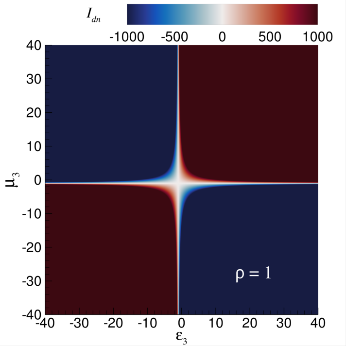
(a)

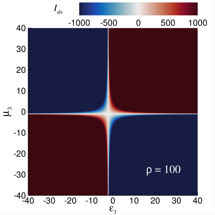
(b)

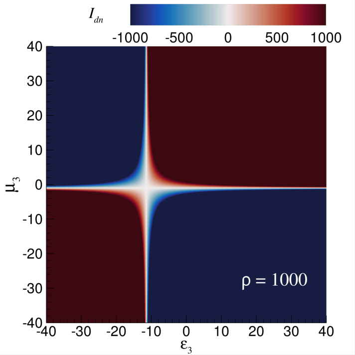
(c)

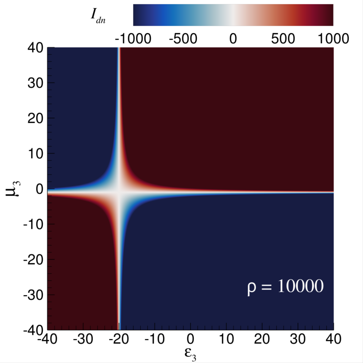
(d)

Figure 2: The variations of $I_{dn}$ (arbitrary unit) when the substrate relative permittivity $\epsilon_{3}$ and permeability $\mu_{3}$ sweep from -40 to -0.1 with the properties of the TI layer being $d_{2}=600$ $\mu\mathrm{m}$, permeability $\mu_{2}=1$, relative permittivity $\epsilon_{2}$=20 and phase $\theta_{2}=\pi$. Each sub-figure corresponds to a distinct value of Hankel transform variable $\rho$. The bright peak features indicate when $I_{dn}$ is close to zero.

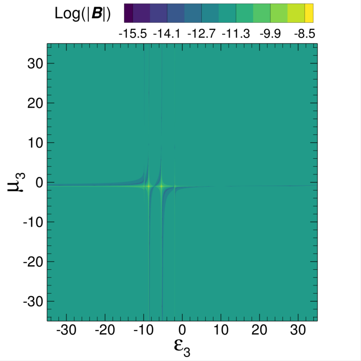
(a) $\epsilon_{2}=10$, $\mu_{2}=1$

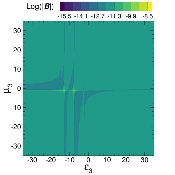
(b) $\epsilon_{2}=15$, $\mu_{2}=1$

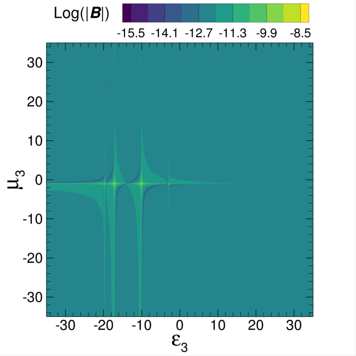
(c) $\epsilon_{2}=20$, $\mu_{2}=1$

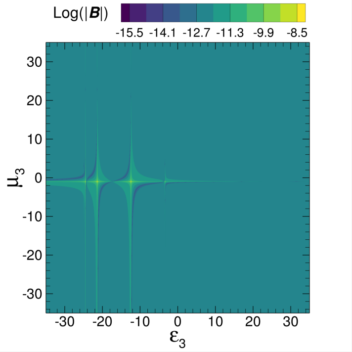
(d) $\epsilon_{2}=25$, $\mu_{2}=1$

Figure 3: The logarithm (base 10) of magnetic field strength, $\log{|\bi{B}|}$ at $z_{\mathrm{ob}}=600$ $\mu\mathrm{m}$, generated by a TI when interfaced due to a 200-elementary-charge point electric source at $d_{1}=2$ $\mu\mathrm{m}$ with various substrates when its relative permittivity $\epsilon_{3}$ and permeability $\mu_{3}$ sweep from -35 to 35. Each sub-figure corresponds to a distinct relative permittivity $\epsilon_{2}$ of the TI layer: (a) $\epsilon_{2}$=10, (b) $\epsilon_{2}$=15, (c) $\epsilon_{2}$=20, and (d) $\epsilon_{2}$=25, while maintaining a constant thickness $d_{2}=600$ $\mu\mathrm{m}$, permeability $\mu_{2}=1$ and $\theta_{2}=\pi$. The bright peak features indicate conditions for maximum magnetic field enhancement, serving as a crucial guide for substrate selection aimed at boosting magnetic responses in TI applications. The sharpness and position of these peaks shift to more negative relative permittivity of the metamaterial substrate with the increase of $\epsilon_{2}$.

To study the magnetic response of a TI-matematerial hybrid structure, we explore the substrate properties when the substrate varies between a standard insulator and a metamaterial with no topological effects ($\theta_{3}=0$). The TI layer was consistently configured with a phase of $\theta_{2}=\pi$, thickness of $d_{2}=600$ $\mu\mathrm{m}$, and a relative permeability of $\mu_{2}=1$. We systematically explore the TI’s relative permittivity, $\epsilon_{2}$, with four values: 10, 15, 20, and 25. The relative permittivity, $\epsilon_{3}$, and permeability, $\mu_{3}$, of the metamaterial substrates were explored over a range from -35 to 35 with a step of 0.05. Our results, which are illustrated in Fig. 3, highlight significant variations in the magnetic field’s amplitude in response to changes in the substrate properties.

Fig. 3 displays the logarithmic magnitude of the magnetic field, $\log{|\bi{B}|}$, at $z_{\mathrm{ob}}=600$ $\mu\mathrm{m}$ generated by an electric point source with 200 elementary charges at $d_{1}=2$ $\mu\mathrm{m}$ as a function of $\epsilon_{3}$ and $\mu_{3}$ of the substrate, These plots indicate possible regions where the magnetic field can be significantly enhanced, appearing as pronounced peaks against a background of relatively low magnetic field intensity. From Fig. 3 (a) to (d), we observe that as the relative permittivity, $\epsilon_{2}$, of the TI layer increases from 10 to 25, the regions of peak enhancement shift to more negative relative permittivity of the metamaterial substrate, suggesting a complex interplay between the TI’s permittivity and the substrate’s properties. Particularly striking are the sharp resonant-like features that indicate conditions under which the magnetic response is markedly amplified.

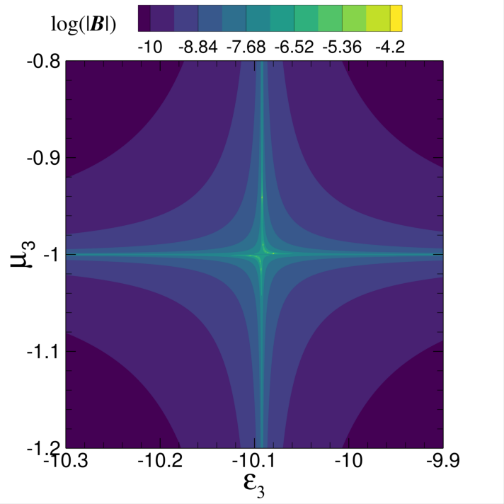
(a)

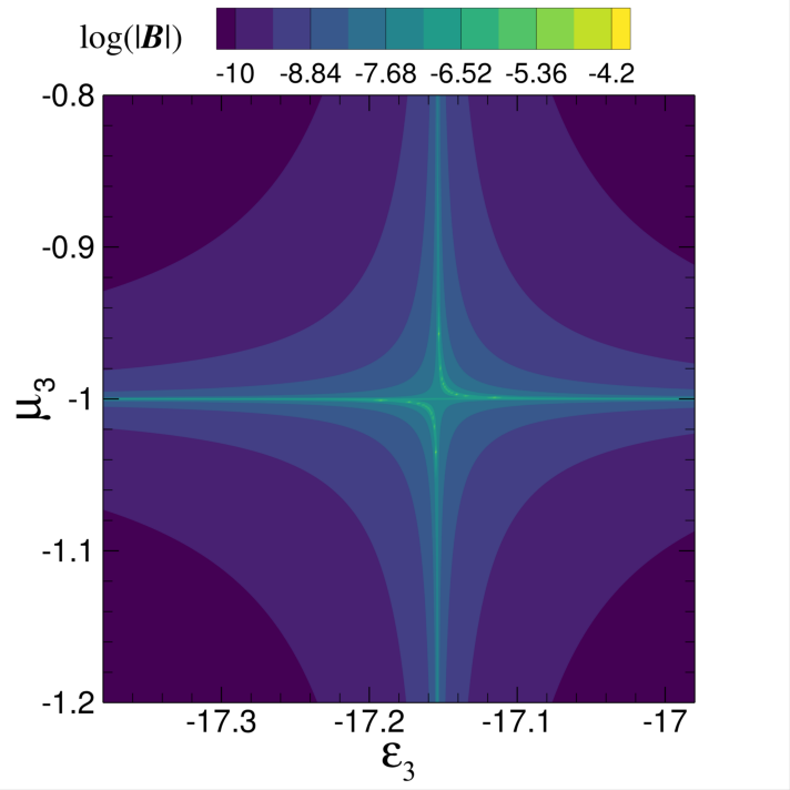
(b)

Figure 4: The logarithm (base 10) of magnetic field strength, $\log{|\bi{B}|}$ at $z_{\mathrm{ob}}=600$ $\mu\mathrm{m}$ due to a TI-metamaterial layer structure generated by a 200-elementary-charge point electric source at $d_{1}=2$ $\mu\mathrm{m}$ when TI is with $d_{2}=600\,\mathrm{}\mu$m, $\theta_{2}=\pi$, $\epsilon_{2}$ = 20 and $\mu_{2}$ = 1; and (a) $\epsilon_{3}\in$ [-10.3, -9.9], $\mu_{3}\in$ [-1.2, -0.8]; (b) $\epsilon_{3}\in$ [-17.4, -17.0], $\mu_{3}\in$ [-1.2, -0.8], with a step of 0.001.

To perform a detailed investigation on the effects of the metamaterial substrate properties on the induced magnetic field in free space, we chose the TI with $d_{2}=600$ $\mu\mathrm{m}$, $\theta_{2}=\pi$, $\epsilon_{2}$ = 20 and $\mu_{2}$ = 1. We then performed a fine sweep of the relative permittivity, $\epsilon_{3}$ and permeability, $\mu_{3}$ with a step of 0.001. From Fig. 3 (c), two sets of regions were identified and studied: (a) $\epsilon_{3}\in$ [-10.3, -9.9], $\mu_{3}\in$ [-1.2, -0.8] and (b) $\epsilon_{3}\in$ [-17.4, -17.0], $\mu_{3}\in$ [-1.2, -0.8]. The corresponding logarithm of magnetic field strength, $\log{|\bi{B}|}$ at $z_{\mathrm{ob}}=600$ $\mu\mathrm{m}$, generated by a 200-elementary-charge point electric source at $d_{1}=2$ $\mu\mathrm{m}$, are shown in Fig. 4. In Fig. 4 (a) with $\epsilon_{3}\in$ [-10.3, -9.9], $\mu_{3}\in$ [-1.2, -0.8], the magnetic field strength in the free space at $z_{\mathrm{ob}}=600$ $\mu\mathrm{m}$ exhibits a symmetric pattern with distinct peaks and valleys around $\epsilon_{3}=-10.092$ and $\mu_{3}=-1$, with maximum at $\epsilon_{3}=-10.08$ $\mu_{3}=-0.999$ which the induced magnetic field strength $|\bi{B}|=249.2$ $\mu$T. In Fig. 4 (b) with $\epsilon_{3}\in$ [-17.4, -17.0], $\mu_{3}\in$ [-1.2, -0.8], the similar pattern shows.

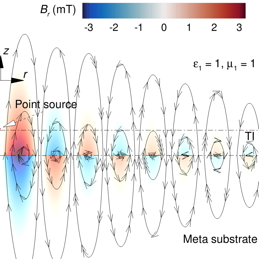
(a)

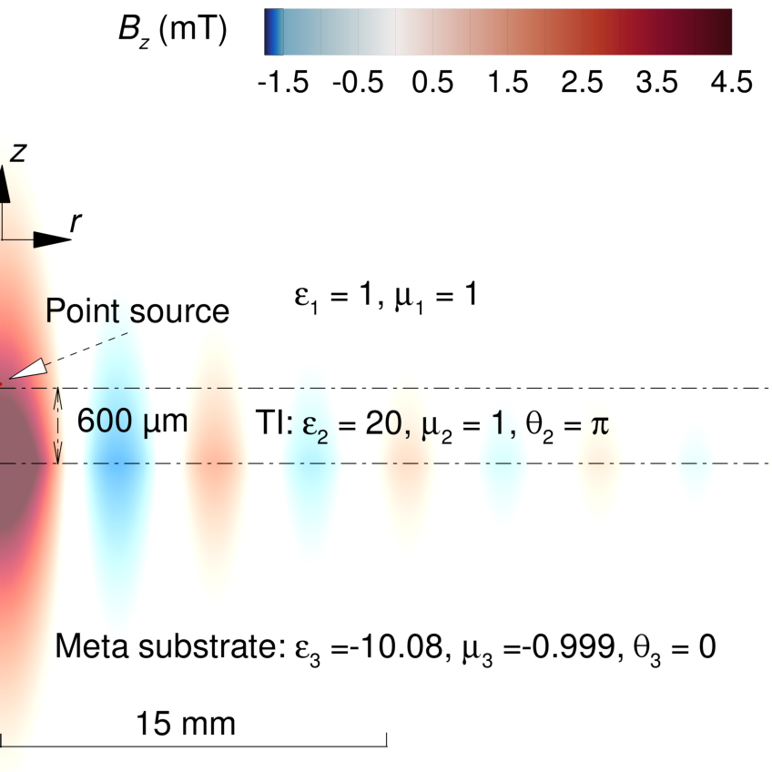
(b)

Figure 5: The distributions of the magnetic field components in the free space, TI and metamaterial substrate, generated by a a 200-elementary-charge point electric source at $d_{1}=2$ $\mu\mathrm{m}$ above TI with $d_{2}=600$ $\mu\mathrm{m}$, $\theta_{2}=\pi$, $\epsilon_{2}$ = 20 and $\mu_{2}$ = 1 on top of a metamaterial substrate with $\epsilon_{3}=-10.08$ and $\mu_{3}=-0.999$: (a) $r$ component and (b) $z$ component.

For the case when the metamaterial’s permittivity and permeability are $\epsilon_{3}=-10.08$ $\mu_{3}=-0.999$, respectively, the $r$ component and $z$ component of the induced magnetic field by a 200-elementary-charge point electric source at $d_{1}=2$ $\mu\mathrm{m}$ in the free space, inside TI and within the metamaterial substrate are shown in Fig. 5, in which the properties of TI are $d_{2}=600$ $\mu\mathrm{m}$, $\theta_{2}=\pi$, $\epsilon_{2}$ = 20 and $\mu_{2}$ = 1, respectively. It is shown clearly that in this case, the magnetic field is significantly enhanced at the interface between the TI layer and metamaterial substrate, which radiates into the free space. Along the $r$ direction, the $z$ component of the induced magnetic field oscillates with dumping which is consistent with the field driven by a point source, and its maximum occurs at the axis-symmetric axis where the point source is located. The $r$ component of the magnetic field behaves similarly to the $z$ component but its oscillation is out of phase with respect to the $z$ component. Along the $z$ direction, the $z$ component is continuous across the TI and metamaterial interface due to the continuity of the normal component of the magnetic field, while the $r$ component is in the opposite direction on the two sides of the interface due to the differences of the relative permittivity and permeability of the TI and metamaterial, in particular the negative relative permittivity and permeability with the metamaterial.

The magnetic field in the free space decreases in an exponential trend as the observation location moves away from the TI surface, as shown in Fig. 6 (a). This gives us a relatively large region in the free space with relatively high magnetic field. On the contrary, for the substrate as a normal insulator with the almost the same magnitude of the relative permittivity and permeability, $\epsilon_{3}=10.08$ and $\mu_{3}=1.000$, respectively, the magnetic field amplitude is the very small even next to the TI surface, which decays nearly in a quadratic trend as the observation location moves away from the TI surface, as presented in Fig. 6 (b).

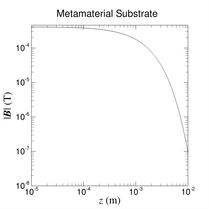
(a) $\epsilon_{3}=-10.08$, $\mu_{3}=-0.999$

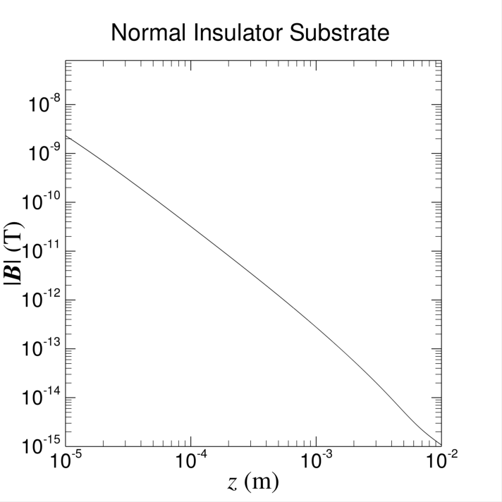
(b) $\epsilon_{3}=10.08$, $\mu_{3}=1.000$

Figure 6: The magnetic field strength, $|\bi{B}|$ at different $z$ when $r=0$, generated by a 200-elementary-charge point electric source at $d_{1}=2\mathrm{}\mu$m a TI with $d_{2}=600\mathrm{}\mu$m, $\theta_{2}=\pi$, $\epsilon_{2}$=20, $\mu_{2}$=1 on: (a) metamaterial substrate with $\epsilon_{3}=-10.08$, $\mu_{3}=-0.999$, (b) normal insulator substrate $\epsilon_{3}=10.08$, $\mu_{3}=1.000$.

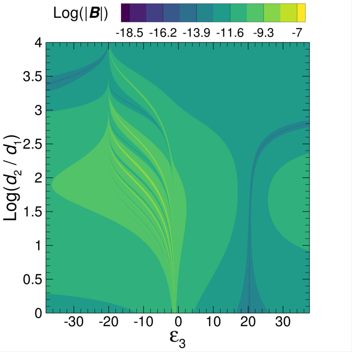
(a) $\mu_{3}=-0.985$

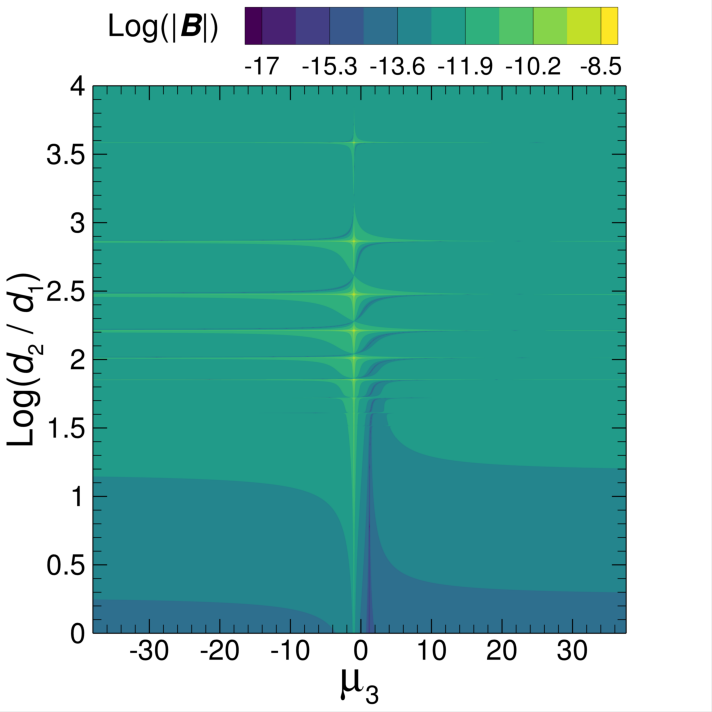
(b) $\epsilon_{3}=-17.15$

Figure 7: The logarithm (base 10) of magnetic field strength, $\log{|\bi{B}|}$ at $z_{\mathrm{ob}}=600$ $\mu\mathrm{m}$, generated by a TI with different thickness when interfaced due to a 200-elementary-charge point electric source at $d_{1}=2$ $\mu\mathrm{m}$ with various substrates when (a) its relative permittivity $\epsilon_{3}$ ranges from -35 to 35 and and (b) its permeability $\mu_{3}$ ranges from from -35 to 35. The bright peak features indicate conditions for maximum magnetic field enhancement, serving as a crucial guide for substrate selection aimed at boosting magnetic responses in TI applications. The number, position and sharpness of these peaks changes significantly due to the thickness of TI and substrate’s relative permittivity and permeability.

We further investigate the effects of TI layer thickness on the induced magnetic field. Fig. 7 provides a detailed analytical view into how the thickness of a TI substrate and the electrical and magnetic properties of the substrate impact the magnetic field produced by an electric point source due to the TI. Two contour maps on the magnetic field that was measured at $z_{\mathrm{ob}}=600$ $\mu\mathrm{m}$ induced by the point electric source with 200 elementary charges located at $d_{1}=2$ $\mu\mathrm{m}$ were included in Fig. 7. Both figures depict the logarithmic magnitude of the magnetic field strength as a function of the TI thickness $d_{2}$ and either the substrate’s relative permittivity $\epsilon_{3}$ in Fig. 7 (a) and its permeability $\mu_{3}$ in Fig. 7 (b).

Fig. 7 (a) shows that the magnetic field strength has a complex dependency on the permittivity of substrate and TI thickness with the permeability fixed at $\mu_{3}$ = -0.985. There are distinct regions where the strength of the magnetic field peaks, visible as bright lines. These peak lines indicate that at certain substrate permittivity, a resonant-like condition is achieved, which significantly enhances the magnetic response. When the thickness of TI is thin around $d_{2}/d_{1}=1$, the most significant enhancement of the magnetic field due to a point electric source concentrate approximate at $\epsilon_{3}=-1.5$. This effect becomes more pronounced and the peak areas broader as the TI layer becomes thicker. Fig. 7 (b) maintains the substrate’s permittivity at $\epsilon_{3}=-17.15$ and varies its permeability and TI thickness. Here, the peak magnetic response shifts in position, implying that the optimal permeability for enhancing the magnetic field also varies with the thickness of the TI layer. There is an indication of optimal bands of permeability at around $\mu_{3}=-1$ which yield the highest magnetic field strength, especially as the TI layer increases in thickness.

Thicker TI layers not only enhance the magnetic field but also offer a broader tolerance for variations in the substrate’s permittivity and permeability. This implies a potential for tuning the system’s sensitivity and performance by adjusting the TI layer’s thickness, which can be critical for designing devices and applications that rely on precise control over magnetic field interactions.

4 Discussion

(a) $\kappa d_{2}=0.01$

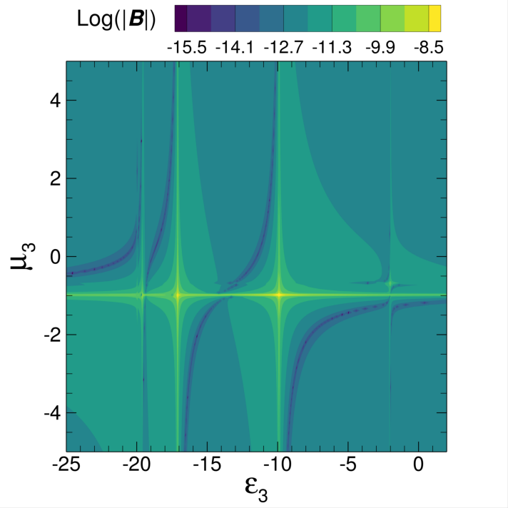
(b) $\kappa d_{2}=0.1$

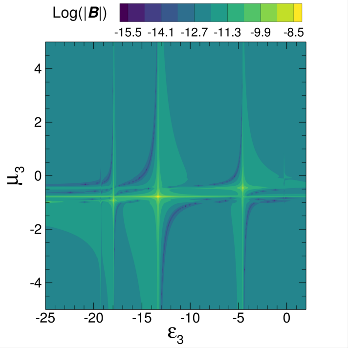
(c) $\kappa d_{2}=1$

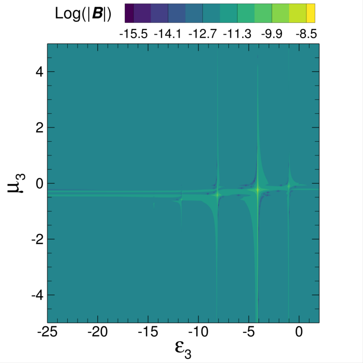
(d) $\kappa d_{2}=5$

Figure 8: The logarithm (base 10) of magnetic field strength, $\log{|\bi{B}|}$ at $z_{\mathrm{ob}}=600$ $\mu\mathrm{m}$, generated by a TI with $d_{2}=600$ $\mu\mathrm{m}$, $\epsilon_{2}$=20, $\mu_{2}=1$ and $\theta_{2}=\pi$ when induced due to a 200-elementary-charge point electric source at $d_{1}=2$ $\mu\mathrm{m}$ on top of various metamaterial substrates with dissipated energy. When $\kappa d_{2}$ is small as in (a) and (b), the magnetic field enhancement in free space behaves nearly the same as when $\kappa\rightarrow 0$, as presented in Sec. 3. When $\kappa d_{2}=1$ as in (c), the magnetic field enhancement in free space due to the metamaterial is also very profound. When $\kappa d_{2}$ is much larger than 1, as in (d), the magnetic field response in free space is suppressed because the energy is absorbed quickly by the metamaterial.

In the previous section, we demonstrated that metamaterials can help enhance the magnetic field response of TIs, in particular when both the relative permittivity and permeability are negative. This can be achieved when these metamaterials are composed of active materials.

There is some discussion that active, non-dissipated materials with negative permittivity and permeability could result in unstable physical systems [35]. To take energy lost into consideration, we modelled that the potentials for both the electric and magnetic fields in the metamaterial domain (domain 3) satisfy the Helmholtz equation, as

$$\nabla^{2}\phi-\kappa^{2}\phi=0$$ (1jklopqt)

where $\phi$ represents either $\phi^{3}_{E}$ or $\phi^{3}_{B}$ in the metamaterial domain, and $1/\kappa$ ($\kappa\gtrapprox 0$) is the characteristic length of energy lost, which is analogous to the skin depth of metallic materials or the Debye length of colloidal systems. When the value of $\kappa$ is low, the energy can be trasmitted deeper into the metamaterial substrate relative to the case when the value of $\kappa$ is high.

In axis-symmetric cases, Eq. (1jklopqt) can also be solved effectively with the Hankel transform [36], which can be written as

$$\frac{\partial^{2}\Phi(\rho,z)}{\partial z^{2}}-(\kappa^{2}+\rho^{2})\Phi(\rho,z)=0$$ (1jklopqu)

for domain 3. As such, we need to rewrite Eq. (1jkl) as

$$\Phi_{E}^{3} =C_{7}\frac{\exp{[\sqrt{\kappa^{2}+\rho^{2}}(z+d_{2})]}}{\sqrt{\kappa^{2}+\rho^{2}}},$$ (1jklopqva)

$$\Phi_{B}^{3} =C_{8}\frac{\exp{[\sqrt{\kappa^{2}+\rho^{2}}(z+d_{2})]}}{\sqrt{\kappa^{2}+\rho^{2}}}.$$ (1jklopqvb)

Correspondingly, to obtain coefficients $C_{7}$ and $C_{8}$ in Eq. (1jklopqv), the first two equations in Eq. (1jklop) need to be updated to

$$\exp{[-\rho d_{2}]}\,C_{3}+C_{5}-\frac{\rho}{\sqrt{\kappa^{2}+\rho^{2}}}C_{7}=0,$$ (1jklopqvwa)

$$\frac{1}{\mu_{2}}\Big{\{}\exp{[-\rho d_{2}]}\,C_{4}+C_{6}\Big{\}}+\frac{\theta_{2}\alpha}{\pi}\frac{1}{c}\Big{\{}\exp{[-\rho d_{2}]}\,C_{3}+C_{5}\Big{\}}-\frac{1}{\mu_{3}}\frac{\rho}{\sqrt{\kappa^{2}+\rho^{2}}}C_{8}=0.$$ (1jklopqvwb)

The results in Fig. 7 indicate that the thickness of the TI has a clear effect on the magnetic field in free space. To demonstrate the competition between the dissipated energy depth in the metamaterial substrate and the thickness of the TI, in Fig. 8, we plot the logarithmic magnitude of the magnetic field, $\log{|\bi{B}|}$, at $z_{\mathrm{ob}}=600\,\mu\mathrm{m}$, generated by an electric point source with 200 elementary charges at $d_{1}=2\,\mu\mathrm{m}$, for different values of $\kappa d_{2}$. The thickness of TI is set to be $d_{2}=600$ $\mu\mathrm{m}$, the relative permittivity $\epsilon_{2}$=20, the relative permeability $\mu_{2}=1$ and the topological phase $\theta_{2}=\pi$. As we can see from Fig. 8 (a) and (b), when $\kappa d_{2}$ is small—indicating the dissipated energy depth in the metamaterial substrate is much larger than the TI thickness—the magnetic field enhancement in free space behaves nearly the same as when $\kappa\rightarrow 0$, as presented in Sec. 3. When $\kappa d_{2}=1$, which means the energy lost depth in the metamaterial substrate is the same as the TI thickness, the magnetic field enhancement in free space due to the metamaterial is also very profound, as shown in Fig. 8 (c). When $\kappa d_{2}$ is much larger than 1, the magnetic field response in free space is suppressed because the energy is absorbed quickly by the metamaterial.

5 Conclusions

This study demonstrates the magnetic field enhancement from a TI driven by an electric point source using TI-metamaterial structures. Through detailed simulations and analysis, it was found that by carefully selecting the permittivity and permeability of the active metamaterial substrate, the induced magnetic field at the interface between the TI layer and the active metamaterial can be significantly enhanced, such as from a few pT to a few $\mu$T. This enhancement extends into free space, providing a larger region with a high magnetic field, which is crucial for exploring the novel magnetic field response of TIs. The findings suggest that the proposed TI-metamaterial approach is a viable and effective method for enhancing the magnetic field response of TIs, revealing new aspects of their electromagnetic properties. This method offers a promising pathway for developing advanced materials and further understanding the unique electromagnetic behavior of TIs.

References

References

- [1] M. Z. Hasan and C. L. Kane. Colloquium: Topological insulators. Reviews of Modern Physics, 82(4):3045–3067, November 2010.
- [2] Xiao-Liang Qi and Shou-Cheng Zhang. Topological insulators and superconductors. Reviews of Modern Physics, 83(4):1057–1110, October 2011.
- [3] B Andrei Bernevig. Topological insulators and topological superconductors. Princeton University Press, Princeton, NJ, April 2013.
- [4] Frank Ortmann, Stephan Roche, and Sergio O Valenzuela, editors. Topological insulators. Wiley-VCH Verlag, Weinheim, Germany, May 2015.
- [5] Xiao-Liang Qi, Rundong Li, Jiadong Zang, and Shou-Cheng Zhang. Inducing a magnetic monopole with topological surface states. Science, 323(5918):1184–1187, February 2009.
- [6] A. Martín-Ruiz, M. Cambiaso, and L. F. Urrutia. Green’s function approach to chern-simons extended electrodynamics: An effective theory describing topological insulators. Physical Review D, 92(12), December 2015.
- [7] A. Martín-Ruiz, M. Cambiaso, and L. F. Urrutia. Electromagnetic description of three-dimensional time-reversal invariant ponderable topological insulators. Physical Review D, 94(8), October 2016.
- [8] Yi-Ping Lai, I-Tan Lin, Kuang-Hsiung Wu, and Jia-Ming Liu. Plasmonics in topological insulators. Nanomaterials and Nanotechnology, 4:13, January 2014.
- [9] Pinyuan Wang, Jun Ge, Jiaheng Li, Yanzhao Liu, Yong Xu, and Jian Wang. Intrinsic magnetic topological insulators. The Innovation, 2(2):100098, May 2021.
- [10] Wenchao Tian, Wenbo Yu, Jing Shi, and Yongkun Wang. The property, preparation and application of topological insulators: A review. Materials, 10(7):814, July 2017.
- [11] Chenxi Yue, Shuye Jiang, Hao Zhu, Lin Chen, Qingqing Sun, and David Zhang. Device applications of synthetic topological insulator nanostructures. Electronics, 7(10):225, October 2018.
- [12] Henry F. Legg, Matthias Rößler, Felix Münning, Dingxun Fan, Oliver Breunig, Andrea Bliesener, Gertjan Lippertz, Anjana Uday, A. A. Taskin, Daniel Loss, Jelena Klinovaja, and Yoichi Ando. Giant magnetochiral anisotropy from quantum-confined surface states of topological insulator nanowires. Nature Nanotechnology, 17(7):696–700, May 2022.
- [13] Ralf Fischer, Jordi Picó-Cortés, Wolfgang Himmler, Gloria Platero, Milena Grifoni, Dmitriy A. Kozlov, N. N. Mikhailov, Sergey A. Dvoretsky, Christoph Strunk, and Dieter Weiss. -periodic supercurrent tuned by an axial magnetic flux in topological insulator nanowires. Phys. Rev. Res., 4:013087, Feb 2022.
- [14] Felix Münning, Oliver Breunig, Henry F. Legg, Stefan Roitsch, Dingxun Fan, Matthias Rößler, Achim Rosch, and Yoichi Ando. Quantum confinement of the dirac surface states in topological-insulator nanowires. Nature Communications, 12(1), February 2021.
- [15] L. A. Castro-Enríquez, A. Martín-Ruiz, and Mauro Cambiaso. Topological signatures in the entanglement of a topological insulator-quantum dot hybrid. Scientific Reports, 12(1), December 2022.
- [16] Hao Wu, Aitian Chen, Peng Zhang, Haoran He, John Nance, Chenyang Guo, Julian Sasaki, Takanori Shirokura, Pham Nam Hai, Bin Fang, Seyed Armin Razavi, Kin Wong, Yan Wen, Yinchang Ma, Guoqiang Yu, Gregory P. Carman, Xiufeng Han, Xixiang Zhang, and Kang L. Wang. Magnetic memory driven by topological insulators. Nature Communications, 12(1), October 2021.
- [17] Mengyun He, Huimin Sun, and Qing Lin He. Topological insulator: Spintronics and quantum computations. Frontiers of Physics, 14(4), May 2019.
- [18] Animesh Pandey, Reena Yadav, Mandeep Kaur, Preetam Singh, Anurag Gupta, and Sudhir Husale. High performing flexible optoelectronic devices using thin films of topological insulator. Scientific Reports, 11(1), January 2021.
- [19] Oliver Breunig and Yoichi Ando. Opportunities in topological insulator devices. Nature Reviews Physics, 4(3):184–193, December 2021.
- [20] Eitan Dvorquez, Benjamín Pavez, Qiang Sun, Felipe Pinto, Andrew D. Greentree, Brant C. Gibson, and Jerónimo R. Maze. Perfect conductor and mu-metal enhancement of effects in electromagnetic fields over single emitters near topological insulators. Physical Review B, 110(16), October 2024.
- [21] A. A. Burkov and Leon Balents. Weyl semimetal in a topological insulator multilayer. Physical Review Letters, 107(12), September 2011.
- [22] Tayyaba Aftab and Kashif Sabeeh. Anisotropic magnetic response of weyl semimetals in a topological insulator multilayer. Journal of Applied Physics, 127(16), April 2020.
- [23] S. Ghosh and A. Manchon. Spin-orbit torque in a three-dimensional topological insulator–ferromagnet heterostructure: Crossover between bulk and surface transport. Physical Review B, 97(13), April 2018.
- [24] Tuo Fan, Nguyen Huynh Duy Khang, Soichiro Nakano, and Pham Nam Hai. Ultrahigh efficient spin orbit torque magnetization switching in fully sputtered topological insulator and ferromagnet multilayers. Scientific Reports, 12(1), February 2022.
- [25] N. B. Devlin, T. Ferrus, and C. H. W. Barnes. Magnetic domain walls in antiferromagnetic topological insulator heterostructures. Physical Review B, 104(5), August 2021.
- [26] Hang An, Ran Zeng, Meng Zhang, Haozhen Li, Miao Hu, Qiliang Li, and Xiaodong Zeng. Linear polarization rotation in multilayer topological insulator structures. Optics Communications, 477:126335, December 2020.
- [27] Abbas Ghasempour Ardakani and Zahra Zare. Strong faraday rotation in a topological insulator single layer using dielectric multilayered structures. Journal of the Optical Society of America B, 38(9):2562, August 2021.
- [28] Viktor G Veselago. The electrodynamics of substances with simultaneously negative values of and . Soviet Physics Uspekhi, 10(4):509–514, April 1968.
- [29] Ekmel Ozbay, Kaan Guven, and Koray Aydin. Metamaterials with negative permeability and negative refractive index: experiments and simulations. Journal of Optics A: Pure and Applied Optics, 9(9):S301–S307, August 2007.
- [30] David R. Smith and Norman Kroll. Negative refractive index in left-handed materials. Physical Review Letters, 85(14):2933–2936, October 2000.
- [31] R. A. Shelby, D. R. Smith, and S. Schultz. Experimental verification of a negative index of refraction. Science, 292(5514):77–79, April 2001.
- [32] Liu Liu, Lei Kang, Theresa S. Mayer, and Douglas H. Werner. Hybrid metamaterials for electrically triggered multifunctional control. Nature Communications, 7(1), October 2016.
- [33] Flynn Castles, Julian A. J. Fells, Dmitry Isakov, Stephen M. Morris, Andrew A. R. Watt, and Patrick S. Grant. Active metamaterials with negative static electric susceptibility. Advanced Materials, 32(9), January 2020.
- [34] Hasib Ibne Rahman and Tian Tang. Electric potential of a point charge in multilayered dielectrics evaluated from hankel transform. Journal of Engineering Mathematics, 110(1):63–73, August 2017.
- [35] S. A. Tretyakov and S. I. Maslovski. Veselago materials: What is possible and impossible about the dispersion of the constitutive parameters. IEEE Antennas and Propagation Magazine, 49(1):37–43, February 2007.
- [36] Alexander D Poularikas, editor. Transforms and applications handbook, third edition. Electrical Engineering Handbook. CRC Press, Boca Raton, FL, 3 edition, April 2009.